Review of Ray Theory Applications in Modelling and Imaging - Norsar
Review of Ray Theory Applications in Modelling and Imaging - Norsar
Review of Ray Theory Applications in Modelling and Imaging - Norsar

You also want an ePaper? Increase the reach of your titles
YUMPU automatically turns print PDFs into web optimized ePapers that Google loves.
REVIEW OF RAY THEORY APPLICATIONS IN MODELLING AND<br />
IMAGING OF SEISMIC DATA<br />
HÅVAR GJØYSTDAL, EINAR IVERSEN, RENAUD LAURAIN, ISABELLE LECOMTE, VETLE VINJE, KETIL ÅSTEBØL *<br />
ABSTRACT<br />
Throughout the last twenty years, 3D seismic ray modell<strong>in</strong>g has developed from<br />
a research tool to a more operational tool that has ga<strong>in</strong>ed grow<strong>in</strong>g <strong>in</strong>terest <strong>in</strong> the<br />
petroleum <strong>in</strong>dustry. Various areas <strong>of</strong> application have been established <strong>and</strong> new ones are<br />
under development. Many <strong>of</strong> these applications require a modell<strong>in</strong>g system with flexible,<br />
robust <strong>and</strong> efficient modell<strong>in</strong>g algorithms <strong>in</strong> the core. The present paper reviews the basic<br />
elements <strong>of</strong> such a system, based on the ‘open model’ concept <strong>and</strong> the ‘wavefront<br />
construction’ technique. In the latter, Červený’s dynamic ray trac<strong>in</strong>g is an <strong>in</strong>tr<strong>in</strong>sic part.<br />
The modell<strong>in</strong>g system can be used for generat<strong>in</strong>g ray attributes <strong>and</strong> synthetic<br />
seismograms for realistic 3D surveys with tens <strong>of</strong> thous<strong>and</strong>s <strong>of</strong> shots <strong>and</strong> receivers.<br />
Moreover, some other types <strong>of</strong> application areas are illustrated: Production <strong>of</strong> Green’s<br />
functions for prestack depth migration <strong>and</strong> hybrid modell<strong>in</strong>g (comb<strong>in</strong>ed ray <strong>and</strong> f<strong>in</strong>itedifference<br />
modell<strong>in</strong>g), attribute mapp<strong>in</strong>g <strong>and</strong> illum<strong>in</strong>ation analysis, both for survey<br />
plann<strong>in</strong>g <strong>and</strong> <strong>in</strong>terpretation. F<strong>in</strong>ally, the concepts <strong>of</strong> ‘isochron rays’ <strong>and</strong> ‘velocity rays’<br />
related to seismic isochrons have been <strong>in</strong>troduced recently, with very <strong>in</strong>terest<strong>in</strong>g future<br />
applications.<br />
1. INTRODUCTION<br />
Twenty years ago a small group <strong>of</strong> geophysicists at NORSAR started to develop a new<br />
s<strong>of</strong>tware package, with the ultimate goal <strong>of</strong> simulat<strong>in</strong>g seismic waves <strong>in</strong> 3D geological<br />
models. Some activity on seismic modell<strong>in</strong>g had also been performed prior to that time −<br />
some experiments had been done with various 3D model representation techniques, <strong>and</strong><br />
the first 3D k<strong>in</strong>ematic ray paths had already been tediously calculated by the old IBM 360<br />
<strong>and</strong> drawn on the shaky drum plotter. But at that time, the amplitudes were absent.<br />
The new s<strong>of</strong>tware project was sponsored by the service company Geco (at that time<br />
‘the Geophysical Company <strong>of</strong> Norway’), hav<strong>in</strong>g ambitions <strong>of</strong> becom<strong>in</strong>g a technology<br />
leader on seismic acquisition, process<strong>in</strong>g, <strong>and</strong> <strong>in</strong>terpretation, <strong>and</strong> clearly see<strong>in</strong>g the need<br />
for an advanced tool <strong>in</strong> 3D modell<strong>in</strong>g. In particular, the grow<strong>in</strong>g development <strong>of</strong> 3D<br />
seismic <strong>in</strong>terpretation stations throughout the eighties made the way short to the<br />
construction <strong>of</strong> 3D models. This potentially short l<strong>in</strong>k between <strong>in</strong>terpretation <strong>and</strong><br />
modell<strong>in</strong>g, with the possibility <strong>of</strong> <strong>in</strong>tegrat<strong>in</strong>g velocity estimation (e.g. tomography) <strong>and</strong><br />
time-to-depth conversion (map migration) <strong>in</strong> the process, was one <strong>of</strong> the ma<strong>in</strong><br />
motivations.<br />
From the very beg<strong>in</strong>n<strong>in</strong>g it was quite clear that the wave simulation method on which<br />
the new modell<strong>in</strong>g system was to be built, would have to be ray trac<strong>in</strong>g. With the<br />
* NORSAR, P.O. Box 51, N-2027 Kjeller, Norway<br />
Stud. geophys. geod., 46 (2002), 113−164 113<br />
© 2002 StudiaGeo s.r.o., Prague
H. Gjøystdal et al.<br />
computer speed <strong>in</strong> those days, ray techniques were <strong>in</strong> fact the only practically applicable<br />
ones <strong>in</strong> general 3D structures, <strong>and</strong>, even more important, these techniques possessed<br />
a number <strong>of</strong> properties that were perfectly suited for <strong>in</strong>tegrat<strong>in</strong>g modell<strong>in</strong>g <strong>and</strong><br />
<strong>in</strong>terpretation: the ability <strong>of</strong> calculat<strong>in</strong>g the wave field as labelled ray contributions (or<br />
events), where event attributes like traveltimes, amplitudes, <strong>in</strong>cident angels, etc., could be<br />
obta<strong>in</strong>ed <strong>in</strong> an explicit manner. In addition, the attributes could serve as a basis for<br />
generat<strong>in</strong>g ray theoretical seismograms, which e.g. could be used for evaluat<strong>in</strong>g <strong>and</strong><br />
test<strong>in</strong>g <strong>of</strong> 3D process<strong>in</strong>g schemes. The advantage <strong>of</strong> be<strong>in</strong>g able to explicitly extract the<br />
various wave propagation effects, like geometrical spread<strong>in</strong>g factors,<br />
reflection/transmission effects at <strong>in</strong>terfaces, phase changes at caustics, splitt<strong>in</strong>g <strong>in</strong> various<br />
branches, P- <strong>and</strong> S-wave modes, etc., was very much appreciated. Another important<br />
characteristic <strong>of</strong> the ray method is the ability to locate the propagation <strong>of</strong> energy <strong>in</strong> the<br />
model, mak<strong>in</strong>g the method particularly suited for applications <strong>in</strong> tomographic <strong>in</strong>version.<br />
Moreover, the <strong>in</strong>tuitive nature <strong>of</strong> ray trac<strong>in</strong>g to visualize wave propagation would make<br />
such a modell<strong>in</strong>g system an ideal ‘educational tool’, <strong>in</strong> order to better underst<strong>and</strong> the<br />
complex features <strong>of</strong> seismic reflections <strong>in</strong> 3D complex media.<br />
Two basic issues were strongly addressed <strong>in</strong> the first specification <strong>and</strong> design phase <strong>of</strong><br />
the 3D seismic modell<strong>in</strong>g system:<br />
− a general <strong>and</strong> flexible model representation scheme for the 3D structural (layered)<br />
model with seismic properties, <strong>and</strong><br />
− an efficient ray trac<strong>in</strong>g algorithm that could be <strong>in</strong>tegrated with the model<br />
representation, calculat<strong>in</strong>g both the k<strong>in</strong>ematic <strong>and</strong> dynamic properties <strong>of</strong> the wave<br />
field along various ray paths between given source <strong>and</strong> receiver positions.<br />
With respect to the first issue, it very soon became clear that we had to start more or<br />
less on scratch. No published methods were found that met our needs, even if some ideas<br />
could be obta<strong>in</strong>ed from the relatively new area <strong>of</strong> 3D computer graphics.<br />
With respect to the second issue we were far luckier. In our earlier experiments we had<br />
used theory from the book <strong>of</strong> Červený et al. (1977), e.g. for cod<strong>in</strong>g the<br />
reflection/transmission coefficients at an <strong>in</strong>terface, <strong>and</strong> later Červený <strong>and</strong> Hron (1980)<br />
turned out to be a major reference. The formulation <strong>of</strong> their dynamic ray tracer fit<br />
perfectly <strong>in</strong>to our modell<strong>in</strong>g scheme, <strong>and</strong> conta<strong>in</strong>ed all the necessary <strong>in</strong>gredients we<br />
searched for: calculation <strong>of</strong> rays as well as ray attributes like wavefront curvatures <strong>and</strong><br />
amplitudes along the rays, <strong>in</strong>clud<strong>in</strong>g both the travell<strong>in</strong>g through the cont<strong>in</strong>uous properties<br />
<strong>of</strong> the layers <strong>and</strong> the conversions at the model <strong>in</strong>terfaces. The methods were clearly <strong>and</strong><br />
explicitly formulated, so the way from the mathematics to computer code was mostly<br />
straightforward. In particular the ray-centered coord<strong>in</strong>ate system was very appropriate to<br />
use <strong>and</strong> easy to implement. It is true to say that these basic works <strong>of</strong> Červený (<strong>and</strong> <strong>of</strong><br />
course also later works) formed one <strong>of</strong> the key elements for our work with modell<strong>in</strong>g<br />
s<strong>of</strong>tware throughout the follow<strong>in</strong>g twenty years. Even after convert<strong>in</strong>g from s<strong>in</strong>gle twopo<strong>in</strong>t<br />
ray trac<strong>in</strong>g <strong>in</strong> the eighties to the wavefront construction technique <strong>in</strong> the n<strong>in</strong>eties,<br />
Červený’s formulas still constitute the very ‘heart’ <strong>of</strong> the system.<br />
Until some few years ago we had to realize that the use <strong>of</strong> 3D seismic modell<strong>in</strong>g as an<br />
<strong>in</strong>dustrial tool was rather limited. Throughout the eighties most applications <strong>of</strong> our<br />
modell<strong>in</strong>g systems were devoted to R&D topics, such as produc<strong>in</strong>g synthetic 3D data for<br />
114 Stud. geophys. geod., 46 (2002)
<strong>Review</strong> <strong>of</strong> <strong>Ray</strong> <strong>Theory</strong> <strong>Applications</strong> <strong>in</strong> Modell<strong>in</strong>g <strong>and</strong> Imag<strong>in</strong>g <strong>of</strong> Seismic Data<br />
test<strong>in</strong>g new process<strong>in</strong>g methods, or check<strong>in</strong>g the validity <strong>of</strong> assumptions <strong>and</strong><br />
approximations adopted <strong>in</strong> order to use more simplified models <strong>in</strong> e.g. migration <strong>and</strong><br />
time-to-depth conversion. There seemed to be a relatively high threshold for us<strong>in</strong>g such<br />
‘advanced’ tools on a more rout<strong>in</strong>e basis <strong>in</strong> operational departments <strong>in</strong> the petroleum<br />
<strong>in</strong>dustry. One <strong>of</strong> the reasons was def<strong>in</strong>itely that the establishment <strong>of</strong> 3D ray trac<strong>in</strong>g<br />
models <strong>of</strong> real complex structures required considerable manual work, <strong>and</strong> the two-po<strong>in</strong>t<br />
ray trac<strong>in</strong>g process for real 3D surveys was very computer <strong>in</strong>tensive, both with respect to<br />
time <strong>and</strong> memory.<br />
We clearly realized two basic th<strong>in</strong>gs: firstly, that the new generation <strong>of</strong> modell<strong>in</strong>g<br />
tools had to be more adapted to the structure (topology) <strong>of</strong> the real <strong>in</strong>terpretation data, to<br />
facilitate a flexible model build<strong>in</strong>g, <strong>and</strong> secondly, that the ray calculation process had to<br />
be far more efficient for simulat<strong>in</strong>g surveys with thous<strong>and</strong>s <strong>of</strong> shots <strong>and</strong> receivers. This<br />
led to the development <strong>of</strong> a new model representation, the open model concept, <strong>and</strong> the<br />
wavefront construction method throughout the n<strong>in</strong>eties. In the last years we have<br />
experienced a cont<strong>in</strong>uous growth <strong>of</strong> advanced 3D seismic modell<strong>in</strong>g tools <strong>in</strong> the seismic<br />
<strong>in</strong>dustry.<br />
Two rather ‘classical’ applications <strong>of</strong> the NORSAR ray trac<strong>in</strong>g systems througout<br />
many years have been simple forward modell<strong>in</strong>g to compute synthetic seismograms, <strong>and</strong><br />
various approaches with<strong>in</strong> tomography <strong>and</strong> velocity <strong>in</strong>version, e.g. as described <strong>in</strong><br />
Gjøystdal <strong>and</strong> Urs<strong>in</strong> (1981), Iversen et al. (1994), <strong>and</strong> Iversen <strong>and</strong> Gjøystdal (1996).<br />
Methods for estimat<strong>in</strong>g the velocity field <strong>in</strong> macro models now plays an important role <strong>in</strong><br />
3D prestack depth migration techniques, e.g. see Faye <strong>and</strong> Jeannot (1986), Iversen et al.<br />
(2000), Br<strong>and</strong>sberg-Dahl et al. (2001).<br />
The purpose <strong>of</strong> this paper is to address some important <strong>and</strong> <strong>in</strong>terest<strong>in</strong>g new areas <strong>of</strong><br />
application <strong>of</strong> a modern 3D seismic modell<strong>in</strong>g system, as encountered dur<strong>in</strong>g our last<br />
years’ activity for the petroleum <strong>in</strong>dustry. For the sake <strong>of</strong> completeness, we will first give<br />
a short descriptive review <strong>of</strong> the basic methods <strong>of</strong> model representation <strong>and</strong> wavefront<br />
construction to produce st<strong>and</strong>ard ray (event) attributes <strong>and</strong> synthetic seismograms. We<br />
have then selected a number <strong>of</strong> examples where ray trac<strong>in</strong>g based modell<strong>in</strong>g has been<br />
applied <strong>in</strong> practical studies, <strong>in</strong>clud<strong>in</strong>g hybrid modell<strong>in</strong>g (comb<strong>in</strong><strong>in</strong>g ray trac<strong>in</strong>g <strong>and</strong> f<strong>in</strong>itedifference<br />
schemes), imag<strong>in</strong>g (prestack depth migration), <strong>and</strong> seismic attribute<br />
mapp<strong>in</strong>g/illum<strong>in</strong>ation analysis. F<strong>in</strong>ally, we describe two recently <strong>in</strong>vented ray concepts<br />
(‘isochron rays’ <strong>and</strong> ‘velocity rays’), which we believe will have very <strong>in</strong>terest<strong>in</strong>g<br />
application potentials <strong>in</strong> the future.<br />
2. MODELS FOR RAY TRACING<br />
An essential part <strong>of</strong> a ray trac<strong>in</strong>g system is the subsurface model <strong>in</strong> which to propagate<br />
the rays. We will here discuss three different aspects <strong>of</strong> the model <strong>in</strong> ray trac<strong>in</strong>g:<br />
1. What the rays need to know about the model.<br />
2. The limitations imposed on the model by the ray trac<strong>in</strong>g method.<br />
3. Model representation for seismic ray trac<strong>in</strong>g.<br />
Stud. geophys. geod., 46 (2002) 115
H. Gjøystdal et al.<br />
2.1. What the rays need to know<br />
The task <strong>of</strong> the model is to serve the rays with some basic <strong>in</strong>formation about the<br />
subsurface. What is requested is well def<strong>in</strong>ed <strong>and</strong> quite simple: At any location <strong>in</strong> the<br />
model, the model must provide the ray-tracer with a few parameters concern<strong>in</strong>g the bulk,<br />
material properties, e.g., the value <strong>and</strong> spatial derivatives <strong>of</strong> isotropic P- <strong>and</strong> S-velocity<br />
functions, anisotropy parameters, density, <strong>and</strong> attenuation factors. The tracer must also get<br />
<strong>in</strong>fo about discont<strong>in</strong>uities <strong>in</strong> the properties, that is, about the subsurface <strong>in</strong>terfaces. It must<br />
be <strong>in</strong>formed if there are any potential ray-<strong>in</strong>terface <strong>in</strong>tersections <strong>in</strong> the vic<strong>in</strong>ity, <strong>and</strong>, if<br />
any, the <strong>in</strong>terface normal <strong>and</strong> curvature must be provided.<br />
2.2. <strong>Ray</strong> trac<strong>in</strong>g model limitations.<br />
The ray trac<strong>in</strong>g theory imposes some limitations on the subsurface model (Červený,<br />
1985): To ensure valid rays, the model parameters must be smooth <strong>and</strong> vary slowly. The<br />
limitations are rather vague, as it is hard to set quantitatively what ‘vary slowly’ means.<br />
What really counts is the relative model smoothness with<strong>in</strong> the Fresnel volume around<br />
each ray (Červený <strong>and</strong> Soares, 1992). It is difficult to use this criterion to prepare a valid<br />
model, as the validity depends not only on model parameters, but also on the f<strong>in</strong>al rays<br />
between sources <strong>and</strong> receivers. In practice we stick to a simpler, ad hoc procedure <strong>and</strong><br />
consider the smoothness as a ray-<strong>in</strong>dependent model property. We l<strong>in</strong>k the smoothness <strong>in</strong><br />
a rough manner to the seismic experiment by smooth<strong>in</strong>g properties <strong>and</strong> <strong>in</strong>terfaces so they<br />
vary with longer wavelength than the dom<strong>in</strong>at<strong>in</strong>g wavelength <strong>in</strong> the recorded seismic<br />
signals (Červený, 2001, p.608).<br />
2.3. Model representation for seismic ray trac<strong>in</strong>g.<br />
Different model representations have been developed for seismic ray trac<strong>in</strong>g. The<br />
simplest one is the 1D model with a vertical sequence <strong>of</strong> constant material properties<br />
separated by plane, horizontal layers. A more flexible model is the ‘layer cake’, which is<br />
a similar sequence, but it varies laterally as the properties <strong>and</strong> <strong>in</strong>terfaces are represented as<br />
grids. More comprehensive seismic model representations for ray trac<strong>in</strong>g <strong>in</strong>clude<br />
CAD/CAM-like solid modell<strong>in</strong>g representation (Gjøystdal et al., 1985), <strong>and</strong> models based<br />
on surface patches (Pereyra, 1992). Very advanced model builders <strong>and</strong> ray tracers are<br />
found <strong>in</strong> other fields, like computer graphics, CAD/CAM, <strong>and</strong> the enterta<strong>in</strong>ment <strong>in</strong>dustry,<br />
<strong>and</strong> there are also well-established general purpose model builders <strong>in</strong> the geoscience<br />
<strong>in</strong>dustry, see for example Mallet et al. (1989). However, as discussed below, seismic ray<br />
modell<strong>in</strong>g has some quite specific characteristics <strong>and</strong> sets certa<strong>in</strong> requirements which <strong>in</strong><br />
general are not fully met by models made for other purposes.<br />
In our present 3D modell<strong>in</strong>g system (V<strong>in</strong>je et al., 1999) we have designed <strong>and</strong> tuned<br />
the subsurface model representation specifically to seismic ray modell<strong>in</strong>g. It is designed<br />
for the external model data we might expect, <strong>and</strong> it takes <strong>in</strong>to account the characteristics<br />
<strong>of</strong> ray trac<strong>in</strong>g. An example <strong>of</strong> a 3D ray trac<strong>in</strong>g model is shown <strong>in</strong> Figure 1.<br />
116 Stud. geophys. geod., 46 (2002)
<strong>Review</strong> <strong>of</strong> <strong>Ray</strong> <strong>Theory</strong> <strong>Applications</strong> <strong>in</strong> Modell<strong>in</strong>g <strong>and</strong> Imag<strong>in</strong>g <strong>of</strong> Seismic Data<br />
Fig. 1. Example <strong>of</strong> a 3D ray trac<strong>in</strong>g model; the SEG/EAGE Salt Model (Am<strong>in</strong>zadeh et al., 1997).<br />
A typical subsurface data set <strong>in</strong> seismic modell<strong>in</strong>g is characterized by:<br />
− A number <strong>of</strong> <strong>in</strong>terfaces, <strong>of</strong>ten <strong>of</strong> complex nature<br />
− Material properties vary <strong>in</strong> a general way <strong>in</strong>side the layers.<br />
− Often <strong>in</strong>complete data, imply<strong>in</strong>g that parts <strong>of</strong> <strong>in</strong>terfaces <strong>and</strong> properties are miss<strong>in</strong>g.<br />
<strong>Ray</strong> trac<strong>in</strong>g requires (see Subsections 2.1 <strong>and</strong> 2.2):<br />
− Frequent <strong>and</strong> fast property evaluation <strong>and</strong> ray-<strong>in</strong>terface <strong>in</strong>tersection.<br />
− Cont<strong>in</strong>uous <strong>and</strong> smooth derivatives <strong>of</strong> properties <strong>and</strong> <strong>in</strong>terfaces.<br />
To honour the above po<strong>in</strong>ts we have made the follow<strong>in</strong>g model representation:<br />
In the model there are just two types <strong>of</strong> geometrical elements: <strong>in</strong>terfaces <strong>and</strong><br />
properties. An <strong>in</strong>terface describes the location <strong>of</strong> the discont<strong>in</strong>uity between two different<br />
layers (volumes, blocks) <strong>in</strong> the subsurface. A property represents a cont<strong>in</strong>uous, bulk,<br />
material property <strong>in</strong> a layer, such as isotropic P-velocity. The model is a simple system <strong>of</strong><br />
po<strong>in</strong>ters from <strong>in</strong>terfaces to properties, see Figure 2.<br />
Each <strong>in</strong>terface is represented as a triangular network with explicit normals <strong>and</strong><br />
curvatures associated with every node. This representation comb<strong>in</strong>es the flexibility <strong>of</strong><br />
triangular networks with an approximate solution for the smoothness required <strong>in</strong> ray<br />
trac<strong>in</strong>g. Strictly speak<strong>in</strong>g, dynamic ray trac<strong>in</strong>g requires <strong>in</strong>terfaces with cont<strong>in</strong>uous <strong>and</strong><br />
smooth 1st <strong>and</strong> 2nd derivatives. However, it is very difficult to make a surface<br />
representation that comb<strong>in</strong>es these properties with the flexibility to represent the complex<br />
<strong>in</strong>terfaces prevalent <strong>in</strong> seismic models. To get around this problem, we have ‘de-coupled’<br />
the <strong>in</strong>terface slightly from its derivatives. As a part <strong>of</strong> the <strong>in</strong>terface construction, the<br />
normals <strong>and</strong> curvatures <strong>in</strong> each node are estimated from the shape <strong>of</strong> the surround<strong>in</strong>g<br />
network <strong>and</strong> stored <strong>in</strong> the node. When the normals <strong>and</strong> curvatures <strong>in</strong> an arbitrary po<strong>in</strong>t are<br />
requested, they are <strong>in</strong>terpolated from the pre-computed values associated with the<br />
surround<strong>in</strong>g nodes, by a procedure similar to the one described <strong>in</strong> Mallet et al. (1997).<br />
With this representation normals <strong>and</strong> curvatures are cont<strong>in</strong>uous <strong>and</strong> smooth, but they are<br />
not necessarily strictly the ‘true’ ones for the <strong>in</strong>terface.<br />
Stud. geophys. geod., 46 (2002) 117
H. Gjøystdal et al.<br />
Fig. 2. The model structure. From each side <strong>of</strong> each <strong>in</strong>terface there is a po<strong>in</strong>ter to the bulk<br />
properties that shall be used for rays traced out from that side <strong>of</strong> the <strong>in</strong>terface. Pi, Si, <strong>and</strong> Di are the<br />
P-wave, S-wave, <strong>and</strong> density functions for the same material ‘i’. Each <strong>in</strong>terface is labelled by an<br />
<strong>in</strong>dex ‘j’ (e.g., I1, I2,...).<br />
Fig. 3. <strong>Ray</strong> trac<strong>in</strong>g <strong>in</strong> an open model. Notice the hole <strong>in</strong> the white <strong>in</strong>terface. <strong>Ray</strong> ‘A’ through<br />
the hole is rejected. It starts out <strong>in</strong> properties #3 below the top <strong>in</strong>terface, while at the next ray<strong>in</strong>terface<br />
<strong>in</strong>tersection at the bottom <strong>in</strong>terface, it is expected to arrive through properties #2. <strong>Ray</strong> ‘B’<br />
is accepted, as the properties at the departure from an <strong>in</strong>terface matches the properties at the arrival<br />
po<strong>in</strong>t on the next one.<br />
118 Stud. geophys. geod., 46 (2002)
<strong>Review</strong> <strong>of</strong> <strong>Ray</strong> <strong>Theory</strong> <strong>Applications</strong> <strong>in</strong> Modell<strong>in</strong>g <strong>and</strong> Imag<strong>in</strong>g <strong>of</strong> Seismic Data<br />
The properties are much simpler to represent than the <strong>in</strong>terfaces. Each property for<br />
each layer is a separate, smooth, <strong>and</strong> slowly vary<strong>in</strong>g function, <strong>and</strong> is represented by a tricubic<br />
spl<strong>in</strong>e.<br />
In real case modell<strong>in</strong>g projects there may be small or even big gaps <strong>in</strong> the <strong>in</strong>terpreted<br />
<strong>in</strong>terfaces where data are miss<strong>in</strong>g for some reason. To allow for ray trac<strong>in</strong>g <strong>in</strong> these<br />
<strong>in</strong>complete data, we have developed a concept where the model is ‘open’, see Åstebøl<br />
(1994) <strong>and</strong> V<strong>in</strong>je et al. (1999). A consistency check sorts out <strong>and</strong> rejects rays that have<br />
passed through the <strong>in</strong>valid, <strong>in</strong>complete parts <strong>of</strong> the model, see Figure 3. The open model<br />
concept saves a lot <strong>of</strong> edit<strong>in</strong>g that would otherwise have been required to fill <strong>in</strong> the<br />
miss<strong>in</strong>g parts. The <strong>in</strong>-fill also <strong>in</strong>troduces uncerta<strong>in</strong>ties <strong>in</strong> the modell<strong>in</strong>g, as ray trac<strong>in</strong>g then<br />
is allowed where very little is known about the subsurface.<br />
3. WAVEFRONT CONSTRUCTION (WFC)<br />
3.1. Background<br />
The wavefront construction (WFC) method was <strong>in</strong>troduced for 2D models <strong>in</strong> a paper<br />
by V<strong>in</strong>je et al. (1993b). Dur<strong>in</strong>g the n<strong>in</strong>eties the method was further developed to<br />
accommodate 3D models (V<strong>in</strong>je et al., 1996a,b; V<strong>in</strong>je et al., 1999). Based on the latter<br />
papers we review here the basic pr<strong>in</strong>ciples <strong>and</strong> properties <strong>of</strong> WFC.<br />
WFC is a ray field technique based on conventional seismic ray theory, as described<br />
by Červený <strong>in</strong> a long list <strong>of</strong> papers, lecture notes, <strong>and</strong> books (e.g., Červený, 1985, 2001).<br />
Instead <strong>of</strong> construct<strong>in</strong>g the ray field ray-by-ray, as it is done <strong>in</strong> classic <strong>in</strong>itial-value ray<br />
trac<strong>in</strong>g or two-po<strong>in</strong>t ray trac<strong>in</strong>g, WFC is build<strong>in</strong>g up the ray field wavefront-by-wavefront.<br />
The propagation from one wavefront to the next is based on trac<strong>in</strong>g <strong>of</strong> a large number <strong>of</strong><br />
short ray segments. The basic idea <strong>in</strong> WFC is to ma<strong>in</strong>ta<strong>in</strong> a uniform density <strong>of</strong> ray<br />
segments on the wavefront dur<strong>in</strong>g its propagation. To control the ray density it is now<br />
common to use criteria based on i) the distance between neighbor<strong>in</strong>g rays <strong>and</strong> ii) the<br />
separation <strong>of</strong> wavefront normals related to such rays. Application <strong>of</strong> these criteria on<br />
a wavefront will lead to creation <strong>of</strong> new rays by <strong>in</strong>terpolation.<br />
The WFC method was developed as a consequence <strong>of</strong> the problems aris<strong>in</strong>g <strong>in</strong> twopo<strong>in</strong>t<br />
ray trac<strong>in</strong>g when attempt<strong>in</strong>g to f<strong>in</strong>d all rays connect<strong>in</strong>g a source po<strong>in</strong>t with<br />
a receiver po<strong>in</strong>t. Traditionally this is done us<strong>in</strong>g shoot<strong>in</strong>g or bend<strong>in</strong>g algorithms. In<br />
a variant <strong>of</strong> the shoot<strong>in</strong>g method described by Červený (1985), a fan <strong>of</strong> rays is traced from<br />
the source po<strong>in</strong>t, <strong>and</strong> paraxial extrapolation is used to estimate values at the receiver<br />
po<strong>in</strong>t(s). The ma<strong>in</strong> problem with these approaches is the lack <strong>of</strong> control <strong>of</strong> divergence<br />
between the rays <strong>in</strong> the search fan. Therefore the trade-<strong>of</strong>f between efficiency <strong>and</strong><br />
reliability/robustness may be unfavorable, especially for complicated 3D models.<br />
Dur<strong>in</strong>g the last ten years WFC has proven to be a very powerful tool <strong>in</strong> seismic<br />
modell<strong>in</strong>g <strong>and</strong> imag<strong>in</strong>g. In Kirchh<strong>of</strong>f type migration or similar (see Section 5) estimation<br />
<strong>of</strong> the Green’s functions by forward modell<strong>in</strong>g is <strong>of</strong>ten the bottleneck <strong>of</strong> the whole<br />
procedure. Also <strong>in</strong> velocity estimation <strong>and</strong> <strong>in</strong> survey plann<strong>in</strong>g forward modell<strong>in</strong>g plays an<br />
important role. The advantage <strong>of</strong> the WFC method is that it can do forward modell<strong>in</strong>g <strong>in</strong><br />
complex 3D models <strong>in</strong> reasonable time, <strong>and</strong> still be able to f<strong>in</strong>d all, or a selection <strong>of</strong>,<br />
reflected <strong>and</strong> transmitted events <strong>in</strong> the receiver po<strong>in</strong>ts.<br />
Stud. geophys. geod., 46 (2002) 119
H. Gjøystdal et al.<br />
The orig<strong>in</strong>al WFC technique was developed for isotropic models. Development to take<br />
<strong>in</strong>to account anisotropy has been reported recently (Gibson, 2000; Mispel <strong>and</strong> Williamson,<br />
2001).<br />
3.2. Representation <strong>of</strong> wavefronts<br />
In the papers by V<strong>in</strong>je et al. (1996a,b) it was essential to f<strong>in</strong>d a simple <strong>and</strong> efficient<br />
numerical representation <strong>of</strong> the 3D wavefront (WF). In general, the representation <strong>of</strong> the<br />
WF <strong>in</strong> 3D is somewhat more complicated than <strong>in</strong> 2D, where the rays are situated side by<br />
side along the 2D WF. The term ‘neighbor<strong>in</strong>g’ or ‘adjacent’ ray is more difficult to def<strong>in</strong>e<br />
on a 3D WF where the rays are distributed <strong>in</strong> two directions. Some k<strong>in</strong>d <strong>of</strong> network<br />
connect<strong>in</strong>g the rays on such a 3D WF must be def<strong>in</strong>ed. This <strong>in</strong>ternal order<strong>in</strong>g <strong>of</strong> po<strong>in</strong>ts<br />
(i.e. the <strong>in</strong>tersection po<strong>in</strong>ts between rays <strong>and</strong> WFs) <strong>and</strong> their <strong>in</strong>ternal connection l<strong>in</strong>es can<br />
be termed as the WF topology. As demonstrated by V<strong>in</strong>je et al. (1996a,b)<br />
a triangular network has both a simple topology <strong>and</strong> the ability to adjust to the stretch<strong>in</strong>g<br />
<strong>and</strong> twist<strong>in</strong>g <strong>of</strong> the WF dur<strong>in</strong>g the propagation through the medium. The processes <strong>of</strong><br />
check<strong>in</strong>g, <strong>in</strong>terpolation <strong>and</strong> estimation <strong>of</strong> receiver parameters are made fairly simple us<strong>in</strong>g<br />
this topology.<br />
The ma<strong>in</strong> steps <strong>in</strong> WFC are<br />
3.3. Propagation <strong>of</strong> wavefronts<br />
− Generation <strong>of</strong> an <strong>in</strong>itial WF,<br />
− Propagat<strong>in</strong>g the WF one time step,<br />
− Controll<strong>in</strong>g the density <strong>of</strong> ray segments on the WF,<br />
− Interpolation to f<strong>in</strong>d arrivals <strong>in</strong> the receivers.<br />
Fig. 4. The icosahedron (a) describes the basic network <strong>of</strong> the po<strong>in</strong>t source. In (b) four repeated<br />
<strong>in</strong>terpolations have taken place on the icosahedron. This leads to a polyhedron that consists <strong>of</strong> 2562<br />
nodes (rays), 7680 sides <strong>and</strong> 5120 triangles.<br />
120 Stud. geophys. geod., 46 (2002)
<strong>Review</strong> <strong>of</strong> <strong>Ray</strong> <strong>Theory</strong> <strong>Applications</strong> <strong>in</strong> Modell<strong>in</strong>g <strong>and</strong> Imag<strong>in</strong>g <strong>of</strong> Seismic Data<br />
In order to start WF propagation, an <strong>in</strong>itial (source) WF is necessary. We need<br />
a triangular grid with sides <strong>and</strong> triangles as equal as possible, <strong>and</strong> <strong>in</strong> this respect, an<br />
icosahedron is especially well suited. The icosahedron consists <strong>of</strong> twelve vertices, thirty<br />
sides <strong>and</strong> twenty regular triangles. We let twelve rays from the source po<strong>in</strong>t pass through<br />
the vertices <strong>of</strong> the icosahedron thus creat<strong>in</strong>g the desired triangular network. The angle<br />
between neighbor<strong>in</strong>g rays <strong>in</strong> this network is then approximately 63.43°. In order to get<br />
a denser sampl<strong>in</strong>g <strong>of</strong> the take<strong>of</strong>f directions we perform <strong>in</strong>terpolation <strong>of</strong> new rays on the<br />
triangular network (the icosahedron). The <strong>in</strong>terpolation is repeated until the criteria for the<br />
density <strong>of</strong> ray segments are fulfilled. In Figure 4 the icosahedron itself <strong>and</strong> the source WF<br />
after four <strong>in</strong>terpolations are plotted.<br />
Assume that a WF represented as a triangular network is present at a time t. For<br />
propagation <strong>in</strong> an isotropic medium (V<strong>in</strong>je et al., 1996a,b) each node (i.e., the<br />
<strong>in</strong>tersections between rays <strong>and</strong> WF) is characterized by a set <strong>of</strong> parameters like:<br />
− Position<br />
− <strong>Ray</strong> tangent<br />
− Take<strong>of</strong>f direction <strong>of</strong> the ray at the source<br />
− Wave mode (e.g. P or S <strong>in</strong> an isotropic medium)<br />
− Unit ray normal <strong>in</strong> the ray-centered coord<strong>in</strong>ate system<br />
− Dynamic parameters such as the P- <strong>and</strong> Q-matrix (Červený, 1985) <strong>and</strong> zero-order ray<br />
amplitude coefficient(s).<br />
Given this set <strong>of</strong> parameters for all nodes at time t, all the rays <strong>in</strong> the WF are traced<br />
a small time step ∆t so that a new WF at time t + ∆t is created. A part <strong>of</strong> the complete<br />
wave field at three successive time steps is plotted <strong>in</strong> Figure 5. The WFs for two time<br />
steps (t <strong>and</strong> t + ∆t) are kept <strong>in</strong> memory to facilitate <strong>in</strong>terpolation <strong>of</strong> new rays <strong>and</strong><br />
estimation <strong>of</strong> event data <strong>in</strong> receivers. All the rays <strong>in</strong> the network are equipped with a userdef<strong>in</strong>ed<br />
ray code which determ<strong>in</strong>es the specific sequence <strong>of</strong> transmissions <strong>and</strong>/or<br />
reflections at the <strong>in</strong>terfaces <strong>in</strong> the model.<br />
Fig. 5. The WF is propagated through the model by trac<strong>in</strong>g all the rays from the old to the new<br />
WF. The WFs for two successive time steps (t <strong>and</strong> t + ∆t) are kept <strong>in</strong> memory.<br />
Stud. geophys. geod., 46 (2002) 121
H. Gjøystdal et al.<br />
Fig. 6. Simple ray cell with an <strong>in</strong>terior receiver. Seismic data are estimated <strong>in</strong> the receiver by<br />
<strong>in</strong>terpolation from the three rays r1 , r2 <strong>and</strong> r3 .<br />
When divergence is present <strong>in</strong> the wave field, parts <strong>of</strong> the WF will be stretched dur<strong>in</strong>g<br />
its propagation through the medium. Both the distance <strong>and</strong> the angular difference <strong>of</strong> ray<br />
tangents between neighbor<strong>in</strong>g rays <strong>in</strong>crease, <strong>and</strong> <strong>in</strong>terpolation is needed <strong>in</strong> order to<br />
ma<strong>in</strong>ta<strong>in</strong> some pre-def<strong>in</strong>ed sampl<strong>in</strong>g density <strong>of</strong> the WF. Several <strong>in</strong>terpolation criteria has<br />
been proposed s<strong>in</strong>ce the first publications on WFC (V<strong>in</strong>je et al. 1992, 1993a, 1993b). For<br />
example, Lambaré‚ et al. (1994) <strong>in</strong>troduced <strong>in</strong>terpolation criteria based on the paraxial ray<br />
approximation (Červený, 1985). Furthermore, V<strong>in</strong>je (1997) <strong>in</strong>troduced an <strong>in</strong>terpolation<br />
criterion based on so-called probe rays that gives control <strong>of</strong> the relative error <strong>of</strong> any<br />
parameter propagated along the WF, but with the cost <strong>of</strong> <strong>in</strong>creased CPU time.<br />
In order to f<strong>in</strong>d arrivals at the receivers we need a procedure able <strong>of</strong> transferr<strong>in</strong>g the<br />
seismic parameters from the mov<strong>in</strong>g WF <strong>in</strong>to each receiver. The volume between two<br />
consecutive WFs (i.e., the old <strong>and</strong> the new WF) is divided <strong>in</strong>to ray cells. These are prism<br />
shaped bodies bounded by three rays <strong>and</strong> the triangle that connects them on each <strong>of</strong> the<br />
two WFs. The six extreme boundaries <strong>of</strong> the spatial coord<strong>in</strong>ates (x, y, z) <strong>of</strong> the ray cell are<br />
used to construct a box that completely conta<strong>in</strong>s the ray cell. Then the subset <strong>of</strong> the<br />
receivers located with<strong>in</strong> the box is found. Some <strong>of</strong> these receivers may also be located<br />
with<strong>in</strong> the ray cell itself. A ray cell with an <strong>in</strong>terior receiver is shown <strong>in</strong> Figure 6. The<br />
seismic parameters for this receiver are found by <strong>in</strong>terpolation from the three rays <strong>of</strong> the<br />
ray cell us<strong>in</strong>g the ray cell coord<strong>in</strong>ates u, v, <strong>and</strong> t*, where (u, v) are the so-called<br />
barycentric coord<strong>in</strong>ates <strong>of</strong> the footpo<strong>in</strong>t <strong>of</strong> the receiver at the base <strong>of</strong> the ray cell, <strong>and</strong> t* is<br />
the traveltime from the base <strong>of</strong> the ray cell to the receiver.<br />
122 Stud. geophys. geod., 46 (2002)
<strong>Review</strong> <strong>of</strong> <strong>Ray</strong> <strong>Theory</strong> <strong>Applications</strong> <strong>in</strong> Modell<strong>in</strong>g <strong>and</strong> Imag<strong>in</strong>g <strong>of</strong> Seismic Data<br />
Fig. 7. An example <strong>of</strong> WF construction <strong>in</strong> an open model. A WF (at 0.9 s) is reflected from the<br />
deepest <strong>in</strong>terface <strong>in</strong> the seismic model. The <strong>in</strong>terface is plotted <strong>in</strong> black while the WF is plotted <strong>in</strong><br />
white. The <strong>in</strong>terface conta<strong>in</strong>s two undef<strong>in</strong>ed areas (holes). Note the hole <strong>in</strong> the WF were it reaches<br />
one <strong>of</strong> the undef<strong>in</strong>ed areas <strong>of</strong> the <strong>in</strong>terface.<br />
3.4. Reflection <strong>and</strong> transmission at <strong>in</strong>terfaces<br />
The open model (see Section 2) is a practical concept for representation <strong>of</strong> realistic<br />
geological models. As shown <strong>in</strong> Figure 7, WF construction can be performed <strong>in</strong> an open<br />
model. The triangular network form<strong>in</strong>g the <strong>in</strong>terfaces possesses the same local<br />
characteristics as the WFs, <strong>and</strong> this can be utilized <strong>in</strong> the process <strong>of</strong> reflect<strong>in</strong>g or<br />
transmitt<strong>in</strong>g a ray at an <strong>in</strong>terface. Each time an <strong>in</strong>tersection between a ray <strong>and</strong> a triangle <strong>of</strong><br />
an <strong>in</strong>terface is detected, the follow<strong>in</strong>g parameters are obta<strong>in</strong>ed for the ray/<strong>in</strong>terface<br />
<strong>in</strong>tersection po<strong>in</strong>t:<br />
− Spatial position: Located <strong>in</strong> the plane between the three vertices <strong>of</strong> the triangle.<br />
Stud. geophys. geod., 46 (2002) 123
H. Gjøystdal et al.<br />
− Interface normal: Interpolated between the three <strong>in</strong>terface normals <strong>in</strong> the vertices <strong>of</strong><br />
the triangle.<br />
− Interface curvature matrix with correspond<strong>in</strong>g local coord<strong>in</strong>ates: Interpolated between<br />
the three curvature matrices <strong>in</strong> the vertices <strong>of</strong> the triangle.<br />
This is sufficient <strong>in</strong>formation to reflect or transmit the ray at the <strong>in</strong>terface, calculat<strong>in</strong>g<br />
both k<strong>in</strong>ematic <strong>and</strong> dynamic parameters.<br />
3.5. WFC <strong>and</strong> multi-arrivals<br />
We consider a model with a s<strong>in</strong>gle <strong>in</strong>terface separat<strong>in</strong>g two homogeneous isotropic<br />
half-spaces. In this model WFC is used for computation <strong>of</strong> reflected contributions<br />
correspond<strong>in</strong>g to a straight receiver l<strong>in</strong>e (see Figure 8a-b). The curvatures <strong>of</strong> the <strong>in</strong>terface<br />
give rise to triplication <strong>of</strong> the depart<strong>in</strong>g WFs <strong>and</strong> thus to multi-arrivals at the receivers<br />
(more than one event per receiver). Examples <strong>of</strong> multi-arrivals for the source <strong>in</strong> Figure 8b<br />
are plotted <strong>in</strong> Figure 9. Four event parameters for the receiver l<strong>in</strong>e are shown: traveltime,<br />
take<strong>of</strong>f angle from the source, amplitude coefficient <strong>and</strong> ray direction at the receivers. The<br />
bow-tie <strong>in</strong> the lower part <strong>of</strong> Figure 9a is the traveltime <strong>of</strong> flank energy which could not be<br />
present <strong>in</strong> any 2D modell<strong>in</strong>g. These arrivals are nicely unfolded <strong>in</strong>to an oval curve <strong>in</strong> the<br />
take<strong>of</strong>f direction plot <strong>in</strong> Figure 9b. In Figure 10, the error (<strong>in</strong> milliseconds) <strong>of</strong> the<br />
traveltime calculations are plotted. The figure shows the difference between the<br />
traveltimes computed by the WF construction <strong>and</strong> the traveltime <strong>of</strong> rays traced from the<br />
source po<strong>in</strong>t to each receiver position. An error <strong>of</strong> maximum 0.2 − 0.3 ms, as showed <strong>in</strong><br />
the figure, is sufficiently small for most geophysical applications. Us<strong>in</strong>g the traveltime<br />
<strong>and</strong> amplitude data from the receivers, a synthetic seismogram is computed (Figure 11).<br />
A 50 Hz Berlage pulse was used <strong>in</strong> the generation <strong>of</strong> the traces. Amplitude variations as<br />
well as phase shifts may be observed <strong>in</strong> the seismogram.<br />
3.6. Computation efficiency − parallel WFC.<br />
The CPU time <strong>of</strong> the WF construction method depends on factors such as the<br />
complexity <strong>of</strong> the model, the sampl<strong>in</strong>g <strong>of</strong> the wavefield (controlled by the user def<strong>in</strong>ed ray<br />
density <strong>and</strong> time-step length), total time propagated, <strong>and</strong> number <strong>of</strong> receivers. A general<br />
observation regard<strong>in</strong>g the CPU time is that the efficiency <strong>in</strong>creases considerably with<br />
number <strong>of</strong> receivers <strong>in</strong> the model compared to traditional two-po<strong>in</strong>t search strategies. To<br />
make simulation <strong>of</strong> large realistic 3D surveys feasible (tens <strong>of</strong> thous<strong>and</strong>s <strong>of</strong> shots <strong>and</strong><br />
receivers), the survey may be automatically divided <strong>in</strong>to a number <strong>of</strong> <strong>in</strong>dependent subtasks,<br />
with a number <strong>of</strong> shots <strong>in</strong> each, which can be distributed to a number <strong>of</strong> computers<br />
or nodes <strong>in</strong> a network. Each <strong>of</strong> these parallel WFC jobs may apply the pr<strong>in</strong>ciple <strong>of</strong> shot<br />
similarity, tak<strong>in</strong>g advantage <strong>of</strong> the fact that with<strong>in</strong> a given arrival branch <strong>of</strong> the wavefronts<br />
hitt<strong>in</strong>g the receivers, the correspond<strong>in</strong>g ray take<strong>of</strong>f directions will generally vary little<br />
from one shot to the next. This makes it possible to use a strategy <strong>of</strong> send<strong>in</strong>g out<br />
wavefronts only <strong>in</strong> preselected directions for most <strong>of</strong> the shots <strong>in</strong> the survey. Only for<br />
a smaller number <strong>of</strong> ‘master shots’, full wavefronts have to be propagated. This option<br />
may decrease the CPU time drastically.<br />
124 Stud. geophys. geod., 46 (2002)
<strong>Review</strong> <strong>of</strong> <strong>Ray</strong> <strong>Theory</strong> <strong>Applications</strong> <strong>in</strong> Modell<strong>in</strong>g <strong>and</strong> Imag<strong>in</strong>g <strong>of</strong> Seismic Data<br />
Fig. 8. WFs <strong>and</strong> re-traced rays to a straight receiver l<strong>in</strong>e <strong>in</strong> a model with a double s<strong>in</strong>usoidal<br />
reflector. (a) The source po<strong>in</strong>t is located <strong>in</strong> the left part <strong>of</strong> the model at position (0.2, 1.25, 0.2) km.<br />
(b) The source po<strong>in</strong>t is at position (1.25, 1.25, 0.2) km.<br />
Stud. geophys. geod., 46 (2002) 125
H. Gjøystdal et al.<br />
Fig. 9. A selection <strong>of</strong> the parameters recorded <strong>in</strong> for the shot <strong>and</strong> receivers <strong>in</strong> Figure 8b. The<br />
figure shows traveltime (a) <strong>and</strong> log10 <strong>of</strong> the modulus <strong>of</strong> the amplitude coefficient (c) as a function<br />
<strong>of</strong> the distance along the receiver l<strong>in</strong>e. In (b) <strong>and</strong> (d), take<strong>of</strong>f angles from the source <strong>and</strong> ray tangent<br />
angles at the receivers are shown.<br />
126 Stud. geophys. geod., 46 (2002)
<strong>Review</strong> <strong>of</strong> <strong>Ray</strong> <strong>Theory</strong> <strong>Applications</strong> <strong>in</strong> Modell<strong>in</strong>g <strong>and</strong> Imag<strong>in</strong>g <strong>of</strong> Seismic Data<br />
Fig. 10. Error <strong>in</strong> traveltime correspond<strong>in</strong>g to the traveltime curve <strong>in</strong> Figure 9a. The difference<br />
between the result <strong>of</strong> WF construction <strong>and</strong> the direct trac<strong>in</strong>g between the source <strong>and</strong> the receivers<br />
has been plotted.<br />
Fig. 11. Synthetic seismogram correspond<strong>in</strong>g to the event data shown <strong>in</strong> Figure 9. A 50 Hz<br />
Berlage pulse was used when the traces were computed.<br />
Stud. geophys. geod., 46 (2002) 127
H. Gjøystdal et al.<br />
4. HYBRID RAY TRACING / FINITE-DIFFERENCE MODELLING<br />
Beside ray trac<strong>in</strong>g (RT) for 2D or 3D wave propagation modell<strong>in</strong>g <strong>of</strong> the earth’s<br />
structures, f<strong>in</strong>ite-difference (FD) techniques are widely used. Both RT <strong>and</strong> FD have<br />
specific advantages <strong>and</strong> severe drawbacks. They are fundamentally different but they do<br />
<strong>in</strong>tend to solve the same problem, i.e., to simulate acoustic/elastic wave propagation <strong>in</strong> the<br />
earth. Unfortunately, the trend is <strong>of</strong>ten to use only one method <strong>and</strong> ignore the other, while<br />
<strong>in</strong> fact they do complete each other. Each method needs the model to be represented <strong>in</strong><br />
a specific way. However, there are very few seismic models which are optimally suited<br />
for RT or FD. A possible solution would therefore be to apply RT modell<strong>in</strong>g <strong>in</strong> some parts<br />
<strong>of</strong> the models where it is appropriate, <strong>and</strong> FD modell<strong>in</strong>g <strong>in</strong> the rest. We will illustrate such<br />
a hybrid comb<strong>in</strong>ation <strong>of</strong> RT <strong>and</strong> FD to model the wavefield scattered by a chosen target<br />
area <strong>of</strong> the model <strong>and</strong> orig<strong>in</strong>ally developed for oil exploration with seismic modell<strong>in</strong>g <strong>of</strong><br />
reservoirs (Lecomte, 1996; Hokstad et al., 1998; Gjøystdal et al., 1998). FD modell<strong>in</strong>g is<br />
applied at the target itself, which may be too complex to be properly described by RT<br />
models. The rest <strong>of</strong> the propagation, prior to <strong>and</strong> after the FD modell<strong>in</strong>g, is performed by<br />
RT through the calculation <strong>of</strong> Green’s functions (GFs). But before illustrat<strong>in</strong>g the results<br />
<strong>of</strong> this hybrid approach, let us first review the characteristics <strong>and</strong> limitations <strong>of</strong> both RT<br />
<strong>and</strong> FD modell<strong>in</strong>g <strong>and</strong> compare them.<br />
4.1. Why hybrid modell<strong>in</strong>g?<br />
There are many versions <strong>of</strong> both RT <strong>and</strong> FD techniques on the market so we will not<br />
focus on a specific one <strong>in</strong> each case but analyze their overall characteristics. The ma<strong>in</strong><br />
philosophy <strong>of</strong> a hybrid concept is <strong>in</strong>deed to take advantage <strong>of</strong> each class <strong>of</strong> methods,<br />
while try<strong>in</strong>g to significantly reduce their <strong>in</strong>herent drawbacks.<br />
<strong>Ray</strong> trac<strong>in</strong>g (RT) modell<strong>in</strong>g<br />
In ray theory, an asymptotic approximation <strong>of</strong> the exact solution <strong>of</strong> the wave equation<br />
is obta<strong>in</strong>ed by search<strong>in</strong>g for a displacement solution <strong>in</strong> the form <strong>of</strong> a ray series (Červený et<br />
al., 1977). The most common approach is to keep only the first-order term after <strong>in</strong>sert<strong>in</strong>g<br />
this solution <strong>in</strong> the wave equations, thus apply<strong>in</strong>g a high frequency approximation. We<br />
then end up with two separate equations: the Eikonal equation for the traveltime <strong>and</strong> the<br />
first transport equation for the amplitudes. This means <strong>in</strong> theory that the results are valid<br />
for wavelengths significantly smaller than any physical scale <strong>in</strong> the model. In practice RT<br />
is <strong>of</strong>ten more robust than predicted <strong>and</strong> may work well for structures down to one fifth <strong>of</strong><br />
the wavelength. Typical RT models are described by smooth <strong>in</strong>terfaces <strong>and</strong> smooth<br />
velocity fields (see Section 2). Furthermore, RT is event-oriented, imply<strong>in</strong>g that the user<br />
may choose the type <strong>of</strong> waves to be modelled <strong>in</strong> the various layers <strong>and</strong> the type <strong>of</strong><br />
reflection/transmission to occur at <strong>in</strong>terfaces. For this reason RT modell<strong>in</strong>g has become a<br />
useful tool for analysis <strong>of</strong> wave propagation <strong>and</strong> identification <strong>of</strong> arrivals.<br />
The major drawback <strong>of</strong> RT is the high frequency assumption, which may lead to<br />
<strong>in</strong>correct amplitudes for the detailed structures <strong>in</strong> oil exploration. Diffractions can be<br />
modelled approximately, but many other wave phenomena are miss<strong>in</strong>g <strong>in</strong> RT modell<strong>in</strong>g,<br />
such as surface waves, evanescent waves, head waves, <strong>and</strong> so forth. There are also<br />
difficulties <strong>in</strong> the vic<strong>in</strong>ity <strong>of</strong> caustic po<strong>in</strong>ts where RT usually gives artificially high<br />
128 Stud. geophys. geod., 46 (2002)
<strong>Review</strong> <strong>of</strong> <strong>Ray</strong> <strong>Theory</strong> <strong>Applications</strong> <strong>in</strong> Modell<strong>in</strong>g <strong>and</strong> Imag<strong>in</strong>g <strong>of</strong> Seismic Data<br />
amplitudes. The efficiency <strong>of</strong> RT modell<strong>in</strong>g is very model dependent <strong>and</strong> difficult to<br />
predict. Moreover, it may be difficult to know <strong>in</strong> advance what waves to model, except for<br />
general classes such as primary reflections.<br />
In prestack depth migration (see Section 5), where GFs are to be calculated on a dense<br />
grid, classic ray trac<strong>in</strong>g is def<strong>in</strong>itely not efficient enough. A more attractive approach is<br />
the WFC technique exposed <strong>in</strong> Section 3. Efficient GFs calculations are <strong>in</strong>deed a necessity<br />
for RT-FD hybrid modell<strong>in</strong>g, especially <strong>in</strong> 3D, even though the hybrid method requires<br />
a much smaller number <strong>of</strong> calculation po<strong>in</strong>ts than prestack depth migration.<br />
F<strong>in</strong>ite-difference (FD) modell<strong>in</strong>g<br />
While RT is utiliz<strong>in</strong>g an asymptotic solution <strong>of</strong> the wave equation, FD modell<strong>in</strong>g is<br />
based on direct discretization <strong>of</strong> the govern<strong>in</strong>g differential equations. To enhance accuracy<br />
the model parameters, the wavefields, <strong>and</strong> the stress components are sampled on staggered<br />
grids (Virieux, 1984; Virieux, 1986). The length <strong>of</strong> the spatial differential operators may<br />
vary from one po<strong>in</strong>t on each side <strong>of</strong> the po<strong>in</strong>t where the derivatives are to be estimated<br />
(2nd order scheme) to as many po<strong>in</strong>ts as one wishes (Holberg, 1987). The differential<br />
operator <strong>in</strong> time is usually <strong>of</strong> 2nd order. The wavefield obta<strong>in</strong>ed by FD modell<strong>in</strong>g can be<br />
stored either as a snapshot, i.e., at a given time iteration for the whole grid, or as<br />
seismograms at a set <strong>of</strong> receivers, imply<strong>in</strong>g that the wavefield is recorded time step after<br />
time step at specific locations.<br />
F<strong>in</strong>ite-difference calculation are constra<strong>in</strong>ed by two conditions. The stability condition<br />
controls that the time sampl<strong>in</strong>g ∆t is not too large with respect to the smallest grid<br />
sampl<strong>in</strong>g ∆h follow<strong>in</strong>g a rule <strong>of</strong> the form:<br />
Vmax∆t ≤ α<br />
∆h<br />
where Vmax is the largest velocity <strong>in</strong> the model, usually a P-wave velocity. The other<br />
constra<strong>in</strong>t is the dispersion condition which assure that the smallest wavelength is not<br />
aliased due to a too coarse grid, i.e., a m<strong>in</strong>imum number <strong>of</strong> grid po<strong>in</strong>ts per wavelength is<br />
def<strong>in</strong>ed:<br />
ν<br />
Vm<strong>in</strong><br />
≤ Nm<strong>in</strong><br />
max∆h<br />
Vm<strong>in</strong> is the smallest velocity <strong>in</strong> the model, usually a S-wave velocity if the calculation is<br />
elastic, <strong>and</strong> νmax is the highest frequency <strong>of</strong> the signal. Both α <strong>and</strong> Nm<strong>in</strong> depend on the<br />
f<strong>in</strong>ite-difference scheme <strong>and</strong> more especially on the length <strong>of</strong> the spatial differential<br />
operators.<br />
FD modell<strong>in</strong>g is easy to use <strong>and</strong> always provide a complete wavefield, <strong>in</strong>clud<strong>in</strong>g all<br />
types <strong>of</strong> waves. The major drawback is the cost <strong>of</strong> such modell<strong>in</strong>g which requires both<br />
large computer memory <strong>and</strong> high CPU time, especially <strong>in</strong> 3D. In the latter case, rout<strong>in</strong>e<br />
modell<strong>in</strong>g <strong>of</strong> complete surveys are absolutely out <strong>of</strong> question. Besides the cost <strong>of</strong> FD<br />
modell<strong>in</strong>g, one possible problem is the grid representation <strong>of</strong> the model which may not be<br />
able to represent properly a detailed geological structure. This is especially true when long<br />
spatial differential operators are used to <strong>in</strong>crease the efficiency <strong>of</strong> the calculation by<br />
Stud. geophys. geod., 46 (2002) 129<br />
(1)<br />
(2)
H. Gjøystdal et al.<br />
choos<strong>in</strong>g a coarser grid sampl<strong>in</strong>g. Actual <strong>in</strong>terfaces <strong>of</strong> the model will take the form as<br />
‘step-stairs’, <strong>and</strong> this may <strong>in</strong>duce annoy<strong>in</strong>g artificial diffractions. A classic example is<br />
mar<strong>in</strong>e seismics with a gently vary<strong>in</strong>g sea floor. The artificial diffractions generated at<br />
that level may be very strong compared to the deeper scattered wavefields. There are<br />
some f<strong>in</strong>ite-difference schemes tak<strong>in</strong>g <strong>in</strong>to account a given <strong>in</strong>terface to correct this effect<br />
but this significantly complicates the code <strong>and</strong> <strong>in</strong>creases the CPU time. The borders <strong>of</strong> the<br />
grid are also troublesome due to generation <strong>of</strong> artificial reflections. They are generally<br />
conditioned to be absorb<strong>in</strong>g by us<strong>in</strong>g an attenuation zone or apply<strong>in</strong>g one-way paraxial<br />
wave equations (Clayton <strong>and</strong> Enquist, 1977), or a comb<strong>in</strong>ation <strong>of</strong> these two techniques.<br />
But the attenuation zones significantly <strong>in</strong>crease the size <strong>of</strong> the grid, which is especially<br />
prejudicial <strong>in</strong> 3D. The one-way paraxial wave equations used to cancel reflections on the<br />
sides require less memory but the absorption depends on the <strong>in</strong>cidence angle. Even with<br />
good absorb<strong>in</strong>g boundaries, artificial reflections generated by the direct wave may be <strong>of</strong><br />
the same order <strong>of</strong> magnitude as the scattered wavefields <strong>of</strong> <strong>in</strong>terest, especially for the deep<br />
structures.<br />
RT/FD comparisons<br />
Table 1 summarizes for each modell<strong>in</strong>g approach its characteristics, advantages, <strong>and</strong><br />
drawbacks. It is easy to see that the RT <strong>and</strong> FD approach complete each other very well,<br />
i.e., a drawback <strong>of</strong> FD is <strong>of</strong>ten an advantage <strong>of</strong> RT <strong>and</strong> vice versa. For <strong>in</strong>stance, the wave<br />
selectivity <strong>of</strong> RT is not available with FD, which is act<strong>in</strong>g as a ‘black-box’. At the same<br />
time, this wave selectivity <strong>in</strong> RT obliges the user to def<strong>in</strong>e a priori all possible significant<br />
waves if wish<strong>in</strong>g a complete calculation, while FD does that automatically. Figure 12<br />
shows the result <strong>of</strong> modell<strong>in</strong>g performed with both methods for the same model, survey<br />
<strong>and</strong> source pulse. The model is not complicated <strong>in</strong> terms <strong>of</strong> the number <strong>of</strong> layers but does<br />
show strong fault<strong>in</strong>g. In the RT modell<strong>in</strong>g we requested the direct transmitted wave <strong>and</strong><br />
all primary P-wave reflections, as well as diffractions correspond<strong>in</strong>g to the direct wave.<br />
The diffractions were obta<strong>in</strong>ed us<strong>in</strong>g the theory <strong>of</strong> Klem-Musatov (1994). The FD<br />
modell<strong>in</strong>g was run with absorb<strong>in</strong>g conditions at the surface <strong>in</strong> order to avoid multiples<br />
(the only possibility to reject arrivals <strong>in</strong> FD). To illustrate the wave propagation with<strong>in</strong><br />
RT, direct transmitted wavefronts calculated by the WFC method <strong>and</strong> raypaths from twopo<strong>in</strong>t<br />
RT are superimposed on the model (Figure 12a, top). The ‘holes’ appear<strong>in</strong>g on the<br />
wavefronts when cross<strong>in</strong>g the faulted area due to diffractions (not shown here) or overcritical<br />
<strong>in</strong>cidences (head waves are miss<strong>in</strong>g). A snapshot <strong>of</strong> the FD wavefield at 1.5 s <strong>of</strong><br />
propagation clearly shows a very complicated pattern where the different arrivals are<br />
difficult to analyze (Figure 12b, top). In the FD snapshot we can identify head waves <strong>and</strong><br />
diffractions <strong>in</strong> addition to reflections <strong>and</strong> pure transmission. The RT seismograms<br />
(Figure 12a, bottom) are not complete but give rather good results for the direct<br />
transmitted waves for most <strong>of</strong> the receivers. Later arrivals (primary reflections) are more<br />
discont<strong>in</strong>uous due to the complexity <strong>of</strong> the structure <strong>and</strong> diffractions would be necessary<br />
to avoid sharp cut<strong>of</strong>fs <strong>of</strong> the reflected phases. Other phases may eventually give<br />
significant arrivals, but it is difficult to def<strong>in</strong>e them a priori. On the other h<strong>and</strong>, the FD<br />
seismograms appear to be more complete <strong>and</strong> cont<strong>in</strong>uous, but wave identification is very<br />
difficult. Note the rather strong arrivals at about 2 s for the deepest receivers (Figure 12b,<br />
bottom), or equivalently, consider the phase identified with white arrows on the snapshot<br />
130 Stud. geophys. geod., 46 (2002)
<strong>Review</strong> <strong>of</strong> <strong>Ray</strong> <strong>Theory</strong> <strong>Applications</strong> <strong>in</strong> Modell<strong>in</strong>g <strong>and</strong> Imag<strong>in</strong>g <strong>of</strong> Seismic Data<br />
(Figure 12b, top). These arrivals correspond to an artificial box-side reflection not totally<br />
suppressed by the chosen one-way wave equation absorb<strong>in</strong>g conditions (Reynolds, 1978).<br />
Without a ray analysis, it is very difficult to tell wether or not such arrivals are real. The<br />
CPU cost <strong>of</strong> RT here was very small (below 1 m<strong>in</strong>.) compared to FD (about one hour),<br />
though add<strong>in</strong>g diffractions <strong>in</strong> RT may significantly <strong>in</strong>crease this cost. It is anyway a good<br />
habit to first try RT to better constra<strong>in</strong> wave propagation <strong>in</strong> a model, then apply FD if<br />
CPU <strong>and</strong> memory resources are available, <strong>and</strong> f<strong>in</strong>ally re-use RT to analyze the FD results.<br />
Fig. 12. RT/FD modell<strong>in</strong>g comparisons <strong>in</strong> a complex model <strong>and</strong> with VSP acquisition. (a) RT<br />
modell<strong>in</strong>g with direct transmitted wavefronts <strong>and</strong> a few selected raypaths for both direct<br />
transmission <strong>and</strong> primary reflections (top) <strong>and</strong> seismograms (bottom). (b) FD modell<strong>in</strong>g with<br />
snapshot <strong>of</strong> the wavefield at 1.5 s (top) <strong>and</strong> seismograms (bottom). One artificial left box-side<br />
reflection is identified on both the snapshot (white arrows) <strong>and</strong> the seismograms (dashed l<strong>in</strong>e).<br />
Stud. geophys. geod., 46 (2002) 131
Table 1.<br />
Type <strong>of</strong><br />
modell<strong>in</strong>g<br />
<strong>Ray</strong><br />
trac<strong>in</strong>g<br />
F<strong>in</strong>itedifference<br />
H. Gjøystdal et al.<br />
Model Arrivals Efficiency Accuracy<br />
- <strong>in</strong>terfaces<br />
separat<strong>in</strong>g layers<br />
BUT<br />
- smoothness is<br />
required<br />
- how smooth?<br />
- parameter grids<br />
BUT<br />
- ‘step-stairs’<br />
troubles<br />
- f<strong>in</strong>est detail =<br />
sampl<strong>in</strong>g<br />
- full selectivity<br />
BUT<br />
- what waves to<br />
select?<br />
- no head waves, no<br />
surface waves,<br />
approximate<br />
diffractions<br />
- complete wavefield<br />
BUT<br />
- what is what?<br />
- reflections from the<br />
borders.<br />
- fast<br />
BUT<br />
- model dependent<br />
- decreases with<br />
<strong>in</strong>creas<strong>in</strong>g<br />
complexity,<br />
no. <strong>of</strong> layers, arrivals<br />
- model <strong>in</strong>dependent<br />
BUT<br />
- slow: model size,<br />
model sampl<strong>in</strong>g <strong>and</strong><br />
frequency dependent<br />
- accurate for smooth<br />
models<br />
BUT<br />
- high-frequency<br />
approximation<br />
- caustic problems<br />
- can be controlled<br />
BUT<br />
- stability <strong>and</strong> dispersion<br />
need to be verified,<br />
- constra<strong>in</strong>ed sampl<strong>in</strong>g<br />
<strong>in</strong> time <strong>and</strong> space<br />
4.2. Where <strong>and</strong> how perform a hybrid RT-FD modell<strong>in</strong>g?<br />
In the follow<strong>in</strong>g we consider the idea <strong>of</strong> apply<strong>in</strong>g RT <strong>and</strong> FD successively <strong>in</strong> a hybrid<br />
comb<strong>in</strong>ation. Orig<strong>in</strong>ally developed for typical oil/gas reservoirs found e.g. on the<br />
Norwegian cont<strong>in</strong>ental shelf (mar<strong>in</strong>e seismics), the hybrid technique is suited for<br />
structures with a rather gentle <strong>and</strong> smooth overburden over a more complex <strong>and</strong> possibly<br />
faulted area <strong>in</strong>clud<strong>in</strong>g a reservoir. The overburden will then be the RT modell<strong>in</strong>g doma<strong>in</strong><br />
<strong>and</strong> the target (i.e., the reservoir) will be the FD modell<strong>in</strong>g doma<strong>in</strong>. There is however no<br />
theoretical limitation <strong>of</strong> the hybrid concept to that type <strong>of</strong> structures only. Alternatively,<br />
we could imag<strong>in</strong>e other type <strong>of</strong> structures where the complexity is close to the surface,<br />
while the target itself could be properly described with RT models. This may be more the<br />
case <strong>in</strong> l<strong>and</strong> seismics, for <strong>in</strong>stance <strong>in</strong> Canada.<br />
As orig<strong>in</strong>ally proposed by Lecomte (1996) <strong>in</strong> acoustics, <strong>and</strong> later further developed <strong>in</strong><br />
elastics (Hokstad et al., 1998), the hybrid modell<strong>in</strong>g scheme proceeds <strong>in</strong> three steps as<br />
illustrated <strong>in</strong> Figure 13, assum<strong>in</strong>g that a target has been selected. RT <strong>and</strong> FD is then totally<br />
de-coupled, i.e., the processes are applied successively with communication via well<br />
def<strong>in</strong>ed data sets (e.g. disk files).<br />
First step: The <strong>in</strong>cident wavefield − RT<br />
The WFC technique <strong>of</strong> RT is used to efficiently compute the GFs connect<strong>in</strong>g any shot<br />
<strong>of</strong> the survey to a coupl<strong>in</strong>g l<strong>in</strong>e (2D) or surface (3D). The overburden should fit for RT<br />
modell<strong>in</strong>g, i.e., with proper smoothness <strong>of</strong> <strong>in</strong>terfaces <strong>and</strong> property fields, <strong>and</strong> with no<br />
major fault<strong>in</strong>g which could generate holes <strong>in</strong> the wavefield. At that stage, we benefit from<br />
the wave selectivity <strong>of</strong> RT, i.e., the user chooses what arrivals to send to the target.<br />
Furthermore, we will not suffer from any artificial noise <strong>in</strong> FD such as diffractions at the<br />
sea floor or box-side reflections. Note that <strong>in</strong> most cases the user selects the direct<br />
132 Stud. geophys. geod., 46 (2002)
<strong>Review</strong> <strong>of</strong> <strong>Ray</strong> <strong>Theory</strong> <strong>Applications</strong> <strong>in</strong> Modell<strong>in</strong>g <strong>and</strong> Imag<strong>in</strong>g <strong>of</strong> Seismic Data<br />
transmitted P-wave as the <strong>in</strong>cident wave <strong>and</strong> direct transmission is less sensitive to small<br />
scale fluctuations <strong>of</strong> the <strong>in</strong>terfaces or parameter fields than reflections. Once the GFs are<br />
calculated, any wavelet can be convolved to generate a wavefield <strong>in</strong>cident to the coupl<strong>in</strong>g<br />
l<strong>in</strong>e (Figure 13, step 1). This wavefield can be re-used for any model <strong>of</strong> the target as long<br />
as the velocity structure is not changed above <strong>and</strong> at the coupl<strong>in</strong>g l<strong>in</strong>e. This <strong>in</strong>creases<br />
efficiency for repeated modell<strong>in</strong>g (Gjøystdal et al., 1998).<br />
Second step: The scattered wavefield − FD<br />
The <strong>in</strong>cident wavefield can now propagate through the target via a local FD modell<strong>in</strong>g<br />
(Figure 13, step 2). The goal here is to record the scattered energy com<strong>in</strong>g back from the<br />
structures <strong>in</strong> the target <strong>in</strong> order to send further this energy towards the receivers <strong>in</strong> the<br />
third step. A special treatment must be applied to prevent the <strong>in</strong>cident wavefield to<br />
propagate upwards, act<strong>in</strong>g as an artificial reflection from the coupl<strong>in</strong>g l<strong>in</strong>e. Complete<br />
boundary conditions may be used to constra<strong>in</strong> the propagation downwards (Hokstad et al.,<br />
1998). Alternatively, the scattered field from a background target model, with no<br />
scatter<strong>in</strong>g structures below the coupl<strong>in</strong>g l<strong>in</strong>e, may be subtracted. The ga<strong>in</strong> <strong>in</strong> cost, with<br />
respect to a classic global FD modell<strong>in</strong>g, is directly proportional to the reduction <strong>in</strong> size <strong>of</strong><br />
the FD-grid times the reduction <strong>in</strong> number <strong>of</strong> time iterations as the <strong>in</strong>terest<strong>in</strong>g time<br />
w<strong>in</strong>dow is shorter. We will here benefit from FD modell<strong>in</strong>g <strong>and</strong> get a complete scattered<br />
wavefield, which was however generated from the <strong>in</strong>cident field explicitly chosen at the<br />
first stage. We thus ga<strong>in</strong> partly the flexibility <strong>of</strong> RT <strong>in</strong> choos<strong>in</strong>g waves: we can for<br />
<strong>in</strong>stance study the difference <strong>in</strong> illum<strong>in</strong>ation <strong>of</strong> a target by primary reflections <strong>and</strong> sea<br />
floor generated multiples. The local FD modell<strong>in</strong>g can be easily applied <strong>in</strong> parallel for<br />
different target models, <strong>and</strong> distributed to a network <strong>of</strong> computers without requir<strong>in</strong>g huge<br />
capacity <strong>in</strong> CPU <strong>and</strong> memory.<br />
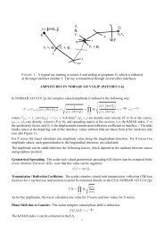
Fig. 13. Scheme <strong>of</strong> the three-step process <strong>of</strong> the hybrid RT-FD modell<strong>in</strong>g. (1) Incident field<br />
calculation us<strong>in</strong>g RT calculated GFs. (2) Scattered field calculation <strong>in</strong> the target with a local FD.<br />
(3) Recorded field calculation at the receivers us<strong>in</strong>g Kirchh<strong>of</strong>f <strong>in</strong>tegral <strong>and</strong> RT calculated GFs.<br />
Stud. geophys. geod., 46 (2002) 133
H. Gjøystdal et al.<br />
Fig. 14. Example <strong>of</strong> the three-step process (acoustic). (1) Incident field to the local FD box with<br />
coupl<strong>in</strong>g at the top. (2) Scattered field com<strong>in</strong>g out from the local FD. (3) Recorded field after<br />
wavefield extrapolation <strong>of</strong> the scattered wavefield us<strong>in</strong>g Kirchh<strong>of</strong>f <strong>in</strong>tegral.<br />
Third step: The recorded wavefield − RT<br />
In the last step, the scattered wavefield emerg<strong>in</strong>g from the local FD-grid is propagated<br />
further towards the receivers by us<strong>in</strong>g the Kirchh<strong>of</strong>f <strong>in</strong>tegral <strong>and</strong> GFs connect<strong>in</strong>g the<br />
coupl<strong>in</strong>g l<strong>in</strong>e to these receivers (Figure 13, step 3). We then aga<strong>in</strong> benefit from RT<br />
selectivity by choos<strong>in</strong>g the paths to follow, i.e., direct transmitted P or direct transmitted<br />
S, <strong>and</strong> so on.<br />
To summarize the hybrid RT-FD modell<strong>in</strong>g, Figure 14 shows a model <strong>in</strong>spired from<br />
exist<strong>in</strong>g structures <strong>in</strong> the North Sea, with the wavefield attached to each step <strong>of</strong> the<br />
process, the coupl<strong>in</strong>g l<strong>in</strong>e be<strong>in</strong>g at the top <strong>of</strong> the FD-grid <strong>in</strong> that example (not required <strong>in</strong><br />
general). In order to check the validity <strong>of</strong> the results, we can compare seismograms<br />
obta<strong>in</strong>ed with RT (Figure 15a), FD (Figure 15b), <strong>and</strong> the hybrid modell<strong>in</strong>g (Figure 15c).<br />
The latter gave a more complete result than RT <strong>and</strong> a better result than the pure FD<br />
(notice the box-side reflections appear<strong>in</strong>g <strong>in</strong> Figure 15b), but at a much cheaper price. The<br />
cost <strong>of</strong> hybrid modell<strong>in</strong>g is about 20% <strong>of</strong> the global FD at the most, although the<br />
parameters were not optimally chosen because we kept the same grid sampl<strong>in</strong>g for the<br />
pure (global) FD <strong>and</strong> the local FD (<strong>in</strong>herent <strong>in</strong> the hybrid approach). In practice, the<br />
optimum grid sampl<strong>in</strong>g depend on the smallest velocity, which is <strong>of</strong>ten located close to<br />
134 Stud. geophys. geod., 46 (2002)
<strong>Review</strong> <strong>of</strong> <strong>Ray</strong> <strong>Theory</strong> <strong>Applications</strong> <strong>in</strong> Modell<strong>in</strong>g <strong>and</strong> Imag<strong>in</strong>g <strong>of</strong> Seismic Data<br />
Fig. 15. Comparison <strong>of</strong> RT, FD <strong>and</strong> hybrid RT-FD results. (a) Classic two-po<strong>in</strong>t RT modell<strong>in</strong>g (no<br />
diffractions). (b) Classic acoustic FD modell<strong>in</strong>g <strong>of</strong> the whole model. (c) Hybrid RT-FD modell<strong>in</strong>g<br />
<strong>of</strong> the target.<br />
the surface. Thereby, the grid sampl<strong>in</strong>g can be coarser for a deep local FD modell<strong>in</strong>g than<br />
for a global FD modell<strong>in</strong>g. Alternatively, one may wish to use the hybrid RT-FD<br />
modell<strong>in</strong>g for detailed models <strong>of</strong> the target, i.e., with sampl<strong>in</strong>g down to just a few meters,<br />
especially vertically. This may be necessary for a proper representation <strong>of</strong> the model as<br />
deduced from well <strong>in</strong>formation. For global FD the cost is then very high because this<br />
sampl<strong>in</strong>g is to be used all over the grid.<br />
Studies carried out the last years show that, even <strong>in</strong> 2D, the hybrid RT-FD modell<strong>in</strong>g<br />
concept may be very powerful for detailed reservoir modell<strong>in</strong>g, especially for 4D studies<br />
with repeated modell<strong>in</strong>g where only the target is to be modified (only the local FD is<br />
affected).<br />
5. PRESTACK DEPTH MIGRATION AND RAY THEORY<br />
Integral approaches us<strong>in</strong>g pre-calculated Green’s functions (GFs) are popular<br />
techniques <strong>in</strong> seismic imag<strong>in</strong>g s<strong>in</strong>ce the eighties (Schneider, 1978; Beylk<strong>in</strong>, 1985;<br />
Bleiste<strong>in</strong>, 1987; Miller et al., 1987). Though significant differences exist <strong>in</strong> the way the<br />
problem is solved, all <strong>in</strong>tegral approaches are usually regrouped under the general term <strong>of</strong><br />
Kirchh<strong>of</strong>f migration (Claerbout, 1985). Some do rely on the Kirchh<strong>of</strong>f <strong>in</strong>tegral, which is<br />
used for backward wavefield extrapolation from the receiver l<strong>in</strong>e/surface. This<br />
Stud. geophys. geod., 46 (2002) 135
H. Gjøystdal et al.<br />
extrapolated wavefield is then correlated to the propagated source wavefield to extract the<br />
reflectivity at a po<strong>in</strong>t (Schneider, 1978). Note that the ‘true’ Kirchh<strong>of</strong>f <strong>in</strong>tegral, strictly<br />
speak<strong>in</strong>g, applies only <strong>in</strong> the constant-velocity case (Claerbout, 1985). Moreover, this<br />
<strong>in</strong>tegral is <strong>in</strong> practice not used directly as it requires knowledge <strong>of</strong> both pressure <strong>and</strong><br />
particle velocity data on a closed surface (Berkhout, 1980). But, assum<strong>in</strong>g a horizontal <strong>and</strong><br />
flat record<strong>in</strong>g l<strong>in</strong>e/surface, <strong>Ray</strong>leigh <strong>in</strong>tegrals are derived from the Kirchh<strong>of</strong>f <strong>in</strong>tegral <strong>and</strong><br />
the <strong>in</strong>tegration is easier, with <strong>of</strong>ten further simplifications where near-field <strong>and</strong> secondorder<br />
terms are neglected. The other type <strong>of</strong> methods (Beylk<strong>in</strong>, 1985; Bleiste<strong>in</strong>, 1987;<br />
Miller et al., 1987), based on <strong>in</strong>version theory <strong>and</strong> Born approximation, takes also the<br />
form <strong>of</strong> ‘a Kirchh<strong>of</strong>f migration <strong>of</strong> frequency filtered <strong>and</strong> spatially weighted traces, with an<br />
<strong>in</strong>tegral kernel dictated by <strong>in</strong>version theory’ (Bleiste<strong>in</strong>, 1987). These techniques are<br />
sometimes called Born migration, though aga<strong>in</strong> usually considered as belong<strong>in</strong>g to the<br />
Kirchh<strong>of</strong>f migration family. In recent years, the term <strong>of</strong> diffraction-stack (DS) migration<br />
has also emerged <strong>in</strong> the Kirchh<strong>of</strong>f migration family, attention be<strong>in</strong>g focused on preserv<strong>in</strong>g<br />
the amplitudes dur<strong>in</strong>g the migration by properly remov<strong>in</strong>g geometrical spread<strong>in</strong>g,<br />
transmission loss <strong>and</strong> caustics effects (Hubral et al., 1991; Schleicher et al., 1993;<br />
Hanitzsch et al., 1994). At last, another <strong>in</strong>tegral approach, called generalized diffraction<br />
tomography (GDT) was developed under the Born or Rytov approximations (Devaney<br />
<strong>and</strong> Zhang, 1991; Gelius et al., 1991), for heterogeneous background <strong>in</strong> opposition to the<br />
classic diffraction tomography techniques (Devaney, 1982; Wu <strong>and</strong> Toksöz, 1987; Lo <strong>and</strong><br />
Toksöz, 1988), <strong>and</strong> was orig<strong>in</strong>ally used for transmission-mode geometry <strong>in</strong> cross-well<br />
tomography. GDT is a less well-known technique <strong>in</strong> seismic imag<strong>in</strong>g but Hamran <strong>and</strong><br />
Lecomte (1993) developed a local plane-wavenumber approach <strong>of</strong> GDT <strong>and</strong> showed its<br />
applications <strong>in</strong> reflection-mode geometry (Lecomte, 1999; Lecomte et al., 2001).<br />
All Kirchh<strong>of</strong>f migration techniques, either ‘true’ Kirchh<strong>of</strong>f like diffraction-stack, or<br />
Born-type, like GDT, require pre-calculated GFs as provided by ray techniques. The<br />
traveltime is the major parameter necessary for migration. For amplitude-preserv<strong>in</strong>g<br />
migration, amplitudes are also necessary though very <strong>of</strong>ten, as a first choice, the data are<br />
rout<strong>in</strong>ely corrected for a simple spherical divergence <strong>in</strong> order to get similar strength for all<br />
reflectors. The Kirchh<strong>of</strong>f techniques may <strong>of</strong>ten need also to use ray direction <strong>in</strong>formation.<br />
This is the case for the obliquity or directivity factor, i.e., the cos<strong>in</strong>e <strong>of</strong> the angle between<br />
the direction <strong>of</strong> propagation at the receiver <strong>and</strong> the vertical axis (horizontal record<strong>in</strong>g<br />
l<strong>in</strong>es). <strong>Ray</strong> directions are also necessary <strong>in</strong> the Beylk<strong>in</strong> determ<strong>in</strong>ant, i.e., the Jacobian <strong>of</strong><br />
the transformation from image to surface coord<strong>in</strong>ates, where the <strong>in</strong>tegration takes place <strong>in</strong><br />
Born-type approaches (Zhang et al., 2000). Even after tak<strong>in</strong>g <strong>in</strong>to account all the<br />
weight<strong>in</strong>g factors <strong>and</strong> ‘true-amplitude’ (TA) corrections, we may not retrieve directly<br />
from the migrated section the true reflectivity (so the term TA migration is mislead<strong>in</strong>g).<br />
Other effects rema<strong>in</strong>, like resolution (Lecomte <strong>and</strong> Gelius, 1998; Gelius <strong>and</strong> Lecomte,<br />
2000) <strong>and</strong> illum<strong>in</strong>ation (Rosl<strong>and</strong> <strong>and</strong> Drivenes, 2000), without speak<strong>in</strong>g <strong>of</strong> possible<br />
coherent noise <strong>in</strong>terfer<strong>in</strong>g with the structure <strong>and</strong> events not correspond<strong>in</strong>g to the<br />
calculated GFs. As far as illum<strong>in</strong>ation is concerned, a technique was proposed by V<strong>in</strong>je<br />
(2000), where ray trac<strong>in</strong>g is used to correct vary<strong>in</strong>g illum<strong>in</strong>ation <strong>of</strong> a target reflector after<br />
PSDM. <strong>Ray</strong> trac<strong>in</strong>g modell<strong>in</strong>g can also be used <strong>in</strong> a survey plann<strong>in</strong>g stage, <strong>in</strong> order to<br />
control illum<strong>in</strong>ation before any data acquisition <strong>and</strong> PSDM. So, prior, dur<strong>in</strong>g <strong>and</strong> after<br />
migration, ray trac<strong>in</strong>g is a powerful technique which <strong>of</strong>ten helps greatly the user to<br />
136 Stud. geophys. geod., 46 (2002)
<strong>Review</strong> <strong>of</strong> <strong>Ray</strong> <strong>Theory</strong> <strong>Applications</strong> <strong>in</strong> Modell<strong>in</strong>g <strong>and</strong> Imag<strong>in</strong>g <strong>of</strong> Seismic Data<br />
underst<strong>and</strong> what happens <strong>in</strong> seismic imag<strong>in</strong>g. In the follow<strong>in</strong>g we shall illustrate the role<br />
<strong>of</strong> various ray trac<strong>in</strong>g parameters (traveltime, ray direction, amplitude) <strong>in</strong> PSDM.<br />
5.1. Traveltimes <strong>and</strong> imag<strong>in</strong>g<br />
Figure 16a shows a simple model we will use to illustrate the role <strong>of</strong> traveltimes <strong>in</strong><br />
PSDM. This model <strong>in</strong>cludes a salt body <strong>in</strong>trud<strong>in</strong>g a few layers <strong>of</strong> constant velocity <strong>and</strong><br />
with a water layer at the top. The survey is a mar<strong>in</strong>e one with a boat shoot<strong>in</strong>g along<br />
a 2 km l<strong>in</strong>e, every 50 m, <strong>and</strong> with a 1 km streamer (25 m sampl<strong>in</strong>g). The target chosen for<br />
PSDM studies is superimposed. For the GF calculation, a model was created which does<br />
not conta<strong>in</strong> the salt body but is an extrapolation <strong>of</strong> the actual model from the left to the<br />
right side as we will only focus on the left side <strong>of</strong> the salt (Figure 16b). Primary P-wave<br />
reflections from all <strong>in</strong>terfaces were generated by dynamic ray trac<strong>in</strong>g, <strong>and</strong> synthetic<br />
seismograms were calculated by convolv<strong>in</strong>g RT results with a 20 Hz zero-phase Ricker<br />
wavelet (Figure 16c). To emphasize the effect <strong>of</strong> traveltime <strong>in</strong> PSDM, we did not apply<br />
neither the geometrical spread<strong>in</strong>g factor nor the reflection/transmission effects. For the<br />
largest <strong>of</strong>fset <strong>of</strong> the shot record<strong>in</strong>g <strong>of</strong> Figure 16c, 5 arrivals are identified by their raypaths<br />
as given <strong>in</strong> Figure 16d. Around ‘arrival 5’ <strong>in</strong> Figure 16c, there are <strong>in</strong> fact other arrivals<br />
correspond<strong>in</strong>g to a reflection at the left flank <strong>of</strong> the salt, illum<strong>in</strong>ated by the primary<br />
P-wave reflection at the reflector at about 2 km <strong>in</strong> depth (arrival 3 is part <strong>of</strong> this primary<br />
reflection). If we now consider only one trace, i.e., the 1 km <strong>of</strong>fset <strong>of</strong> the shot <strong>of</strong><br />
Figure 16c, traveltime <strong>in</strong>formation <strong>of</strong> GFs will be used to map back to depth the energy <strong>of</strong><br />
the seismograms along isochrons (Figure 16e). As will be discussed further <strong>in</strong> Section 7,<br />
an isochron is a surface <strong>of</strong> constant two-way traveltime correspond<strong>in</strong>g to a s<strong>in</strong>gle shot <strong>and</strong><br />
a s<strong>in</strong>gle receiver. Apply<strong>in</strong>g now DS to the chosen trace, we get the PSDM section <strong>of</strong><br />
Figure 16f where we easily identified our 5 arrivals <strong>of</strong> Figure 16c <strong>and</strong> 16d. Their<br />
respective energy has been mapped along the isochrons <strong>of</strong> Figure 16e, as expected, <strong>and</strong><br />
with the same amplitude all along each isochron <strong>in</strong> our case. Referr<strong>in</strong>g to Figure 16d, we<br />
see however that only arrival 2 corresponds to a reflection <strong>in</strong> our target. Reflections 1,3,4<br />
<strong>and</strong> 5 are all associated with part <strong>of</strong> reflectors outside our target but the correspond<strong>in</strong>g<br />
isochrons cross the latter because one trace is not a sufficient <strong>in</strong>formation to locate energy.<br />
Basically, a PSDM section is formed by superposition <strong>of</strong> such elementary ‘one-trace’<br />
images, the idea be<strong>in</strong>g that, all together, constructive <strong>in</strong>terference will occur at the actual<br />
loci <strong>of</strong> reflections, while the useless part <strong>of</strong> the isochrons will be cancelled by destructive<br />
<strong>in</strong>terference.<br />
Figure 17 shows what happens when several traces are migrated. As very <strong>of</strong>ten done,<br />
data can be migrated <strong>in</strong> constant-<strong>of</strong>fset sections, like <strong>in</strong> Figure 17a (zero-<strong>of</strong>fset) <strong>and</strong> 17b<br />
(1 km <strong>of</strong>fset). The three reflectors <strong>of</strong> the target are com<strong>in</strong>g forward, though we still see<br />
some ‘background pattern’ similar to the isochrons <strong>of</strong> Figure 16f <strong>in</strong> both cases. This is<br />
<strong>of</strong>ten called alias<strong>in</strong>g noise, which is due to a too coarse sampl<strong>in</strong>g between the shots: the<br />
<strong>in</strong>terference is not perfect between the isochrons <strong>and</strong> they do not cancel each other where<br />
they should. By migrat<strong>in</strong>g all shots <strong>and</strong> <strong>of</strong>fsets together, the PSDM section gets much<br />
clearer (Figure 17c), though we can still see what rema<strong>in</strong>s <strong>of</strong> an isochron correspond<strong>in</strong>g to<br />
the salt reflection.<br />
Stud. geophys. geod., 46 (2002) 137
H. Gjøystdal et al.<br />
Fig. 16. Salt model. (a) P-velocity from 1.5 km/s (top) to 4.0 km/s (salt) <strong>and</strong> target location.<br />
(b) Model used for Green’s function calculation. (c) Shot record<strong>in</strong>g at 0 km with <strong>of</strong>fsets from 0 to<br />
1 km every 25 m (right side). (d) Primary reflections at 1 km <strong>of</strong>fset with identification <strong>of</strong> 5 arrivals<br />
(see also c). (e) Scatter<strong>in</strong>g traveltime isochrons for 1 km <strong>of</strong>fset. (f) PSDM section for 1 km <strong>of</strong>fset<br />
with identification <strong>of</strong> the same arrivals as <strong>in</strong> (c) <strong>and</strong> (d).<br />
138 Stud. geophys. geod., 46 (2002)
<strong>Review</strong> <strong>of</strong> <strong>Ray</strong> <strong>Theory</strong> <strong>Applications</strong> <strong>in</strong> Modell<strong>in</strong>g <strong>and</strong> Imag<strong>in</strong>g <strong>of</strong> Seismic Data<br />
Fig. 17. PSDM sections for a survey <strong>of</strong> 41 shots from 0 to 2 km every 50 m, <strong>and</strong> same <strong>of</strong>fset range<br />
as <strong>in</strong> Figure 16. (a) zero-<strong>of</strong>fset section. (b) 1 km <strong>of</strong>fset. (c) All shots <strong>and</strong> <strong>of</strong>fset.<br />
In Kirchh<strong>of</strong>f migration techniques, the choice <strong>of</strong> the traveltimes to use is <strong>of</strong>ten a critical<br />
issue, especially because one arrival per grid po<strong>in</strong>t, <strong>and</strong> only one, is the preferred solution<br />
for the sake <strong>of</strong> efficiency. So, should we use first-arrival (but may be associated with very<br />
low energy), highest-amplitude arrival, shortest-path arrival? There is no absolute answer<br />
to these questions because, ideally, we should use all arrivals to get closer to<br />
the − smooth − result <strong>of</strong> wave equation migration, but aga<strong>in</strong> at the cost <strong>of</strong> efficiency. That<br />
is why some people claim that we will soon be ‘beyond’ Kirchh<strong>of</strong>f imag<strong>in</strong>g, argu<strong>in</strong>g that<br />
the computers are develop<strong>in</strong>g so fast that wave-equation migration will take over. But<br />
Kirchh<strong>of</strong>f migration will get faster as well, so may be we can use all arrivals then?<br />
Gaussian-beam techniques <strong>in</strong> RT may also be a better solution than the ‘s<strong>in</strong>gle-raypath’<br />
solutions provided by most GFs calculators, i.e., with events tak<strong>in</strong>g <strong>in</strong>to account the<br />
surround<strong>in</strong>g structures <strong>in</strong> ‘energy tubes’ where the Fresnel zone is considered. This may<br />
<strong>in</strong>duce a smooth<strong>in</strong>g <strong>of</strong> the GFs (especially their amplitudes) which may greatly improve<br />
the quality <strong>of</strong> PSDM sections, giv<strong>in</strong>g smoother images, like <strong>in</strong> wave-equation migration?<br />
This is def<strong>in</strong>itely an <strong>in</strong>terest<strong>in</strong>g topic <strong>of</strong> research, which is <strong>in</strong>deed a fundamental question<br />
for RT techniques: how does the actual propagation <strong>of</strong> the waves compare to the ray<br />
approach? RT techniques will however always be much more <strong>in</strong>formative about what<br />
happens when perform<strong>in</strong>g migration than FD techniques used for wave-equation<br />
migration, which act as black-boxes. As <strong>in</strong> the previous section we f<strong>in</strong>d here <strong>in</strong>deed the<br />
same arguments both for <strong>and</strong> aga<strong>in</strong>st each technique. One should not systematically reject<br />
one method <strong>in</strong> favor <strong>of</strong> the other one, s<strong>in</strong>ce they may <strong>in</strong>deed complete each other.<br />
Figure 18 is an example illustrat<strong>in</strong>g the flexibility <strong>of</strong> RT techniques <strong>in</strong> case <strong>of</strong> complicated<br />
illum<strong>in</strong>ation <strong>of</strong> a structure. Let us consider the same shot gather as <strong>in</strong> Figure 16c <strong>and</strong><br />
migrate it with direct transmitted waves both from shots <strong>and</strong> towards receivers<br />
(Figure 18a). In agreement with the raypaths showed above, we retrieve only a small part<br />
<strong>of</strong> the salt <strong>in</strong> its upper concave part. Note that the small illum<strong>in</strong>ated zone predicted by rays<br />
is <strong>in</strong> fact larger due to Fresnel zone effects <strong>and</strong> poor vertical resolution. If we now<br />
consider GFs comb<strong>in</strong><strong>in</strong>g the primary reflections at the reflector at about 2 km <strong>in</strong> depth<br />
Stud. geophys. geod., 46 (2002) 139
H. Gjøystdal et al.<br />
Fig. 18. Salt flank imag<strong>in</strong>g with shot at 0 km. (a) <strong>Ray</strong>s attached to primary reflections from salt<br />
(top) <strong>and</strong> PSDM section us<strong>in</strong>g only direct transmission GFs both from shot <strong>and</strong> towards receivers<br />
(bottom). (b) Salt flank illum<strong>in</strong>ated from a primary reflection (top), which is used for GFs<br />
calculation from the shot to get the PSDM section (bottom) while direct transmission is still used<br />
towards the receivers.<br />
from the shots <strong>and</strong> direct transmission towards the receivers, the new PSDM section is<br />
totally different, show<strong>in</strong>g now the nearly vertical left flank <strong>of</strong> the salt. Is there any waveequation<br />
migration technique able to take <strong>in</strong>to account such vertical structures? This is<br />
<strong>in</strong>deed the weakness <strong>of</strong> these approaches, so far, rely<strong>in</strong>g onto paraxial approximations <strong>of</strong><br />
the wave-equation <strong>and</strong> limited dip ranges.<br />
5.2. <strong>Ray</strong> directions <strong>and</strong> imag<strong>in</strong>g<br />
While traveltimes play a very important role <strong>in</strong> migration, by locat<strong>in</strong>g properly <strong>in</strong><br />
depth the recorded seismic energy, other RT parameters are also significant <strong>and</strong> very<br />
<strong>in</strong>formative. We chose here to illustrate the concept <strong>of</strong> the scatter<strong>in</strong>g wavenumber vector<br />
K def<strong>in</strong>ed by:<br />
K = kr −ks<br />
140 Stud. geophys. geod., 46 (2002)<br />
(3)
<strong>Review</strong> <strong>of</strong> <strong>Ray</strong> <strong>Theory</strong> <strong>Applications</strong> <strong>in</strong> Modell<strong>in</strong>g <strong>and</strong> Imag<strong>in</strong>g <strong>of</strong> Seismic Data<br />
Fig. 19. Scatter<strong>in</strong>g wavenumber K. (a) Def<strong>in</strong>ition. (b) K is perpendicular to a reflector if reflection<br />
is attached to it. These two angles are equal if P-wave to P-Wave, respectively S-wave to S-wave,<br />
scatter<strong>in</strong>g, but different if P- to S-wave <strong>and</strong> vice versa.<br />
where ks <strong>and</strong> kr are the two local wavenumbers given <strong>in</strong> Figure 19a, i.e., the wavenumber<br />
attached to the <strong>in</strong>cident field at the considered image po<strong>in</strong>t, respectively the wavenumber<br />
attached to the scattered field at the same po<strong>in</strong>t. This vector, or more precisely its<br />
opposite, was already part <strong>of</strong> the early Born approaches <strong>in</strong> Kirchh<strong>of</strong>f migration (Beylk<strong>in</strong>,<br />
1985). In GDT approaches (Hamran <strong>and</strong> Lecomte, 1993), K is a key parameter which<br />
completely describes the illum<strong>in</strong>ation <strong>and</strong> the resolution at each image po<strong>in</strong>t. Seismic<br />
imag<strong>in</strong>g can <strong>in</strong>deed be assimilated to a generalized Fourier transform (FT) <strong>and</strong> the local<br />
coverage with respect to length <strong>and</strong> orientation <strong>of</strong> K vectors <strong>in</strong>dicates how much<br />
<strong>in</strong>formation we have about the local scatter<strong>in</strong>g properties <strong>of</strong> the structure. The more K<br />
coverage we have, the better is the possibility for illum<strong>in</strong>ation <strong>and</strong> sharp resolution<br />
(Lecomte <strong>and</strong> Gelius, 1998). Furthermore, while most classic <strong>in</strong>tegral approaches apply<br />
a coord<strong>in</strong>ate transformation from the scatter<strong>in</strong>g wavenumber back to the shot <strong>and</strong> receiver<br />
l<strong>in</strong>es, a much simpler approach is to stay <strong>in</strong> a local coord<strong>in</strong>ate system (Figure 19b). This<br />
system is simply polar <strong>in</strong> 2D <strong>and</strong> spherical <strong>in</strong> 3D, <strong>and</strong> this is very similar to what is done<br />
<strong>in</strong> classic spotlight-mode synthetic aperture radar (SAR) imag<strong>in</strong>g (Lecomte et al., 2001).<br />
In a local 2D coord<strong>in</strong>ate system, K is def<strong>in</strong>ed by an orientation angle, <strong>and</strong> a length<br />
function <strong>of</strong> the frequency <strong>and</strong> the angle θ (Figure 19b). If there was a reflection attached<br />
to the wavenumber couple (ks, kr), K is perpendicular to that reflector.<br />
To illustrate the importance <strong>of</strong> the scatter<strong>in</strong>g wavenumber vector, determ<strong>in</strong>ed by RT<br />
from ray directions at the image po<strong>in</strong>t, a realistic model <strong>of</strong> the Gullfaks oil field on the<br />
Norwegian cont<strong>in</strong>ental shelf has been used (Figure 20). Synthetic data correspond<strong>in</strong>g to<br />
the reservoir target <strong>in</strong>dicated <strong>in</strong> Figure 20a, with an oil/water contact, were generated by<br />
the hybrid RT/FD modell<strong>in</strong>g method exposed earlier. Three data set were used to generate<br />
PSDM sections: zero-<strong>of</strong>fset (Figure 20b), far-<strong>of</strong>fset (Figure 20c) <strong>and</strong> all data (Figure 20d).<br />
On the right side <strong>of</strong> the constant-<strong>of</strong>fset sections, the local scatter<strong>in</strong>g wavenumber coverage<br />
at two po<strong>in</strong>ts <strong>of</strong> the target are given. In each case, the white arrow <strong>in</strong>dicates the mean<br />
scatter<strong>in</strong>g wavenumber, i.e., the reflector normal which is best illum<strong>in</strong>ated, while the grey<br />
arrow is the perpendicular to the actual local reflector. In the zero-<strong>of</strong>fset case, reflector 1<br />
is rather poorly illum<strong>in</strong>ated (grey arrow near the border <strong>of</strong> the K coverage <strong>and</strong> far from<br />
Stud. geophys. geod., 46 (2002) 141
H. Gjøystdal et al.<br />
Fig. 20. Illum<strong>in</strong>ation <strong>and</strong> resolution. (a) Model <strong>of</strong> the Gullfaks field on the Norwegian cont<strong>in</strong>ental<br />
shelf with survey (161 shots every 25 m, 100 <strong>of</strong>fsets from 0. to 2475 m) <strong>and</strong> PSDM target. (b) Zero<strong>of</strong>fset<br />
PSDM section with superimposed Po<strong>in</strong>t-Spread functions (PSFs, 100×100 m 2 ) at some<br />
locations (left). Scatter<strong>in</strong>g wavenumber coverage at two reflectors (right). (c) Far-<strong>of</strong>fset PSDM<br />
section. Same as for (b). (d) All shots <strong>and</strong> <strong>of</strong>fsets section with superimposed PSFs. Courtesy <strong>of</strong><br />
Statoil.<br />
the white arrow) while reflector 2 is clearly better illum<strong>in</strong>ated. This is confirmed by the<br />
PSDM section which shows a strong reflector 2 <strong>and</strong> weak reflector 1. This effect is not<br />
only due to the impedance contrast <strong>and</strong> does really reflect the differences <strong>in</strong> illum<strong>in</strong>ation,<br />
as confirmed by the far-<strong>of</strong>fset section which shows now the opposite, i.e., a strong<br />
reflector 1 <strong>and</strong> a non-exist<strong>in</strong>g reflector 2. The latter result is aga<strong>in</strong> <strong>in</strong> agreement with the<br />
illum<strong>in</strong>ation analysis provided by the local K coverages. Note a little ‘alias<strong>in</strong>g-noise’ on<br />
the zero-<strong>of</strong>fset section due to the same effect mentioned <strong>in</strong> Figure 17a.<br />
The local K coverage does not only give <strong>in</strong>formation about illum<strong>in</strong>ation but also about<br />
the expected resolution <strong>of</strong> the <strong>in</strong>version process which is seismic imag<strong>in</strong>g. The FT <strong>of</strong> the<br />
142 Stud. geophys. geod., 46 (2002)
<strong>Review</strong> <strong>of</strong> <strong>Ray</strong> <strong>Theory</strong> <strong>Applications</strong> <strong>in</strong> Modell<strong>in</strong>g <strong>and</strong> Imag<strong>in</strong>g <strong>of</strong> Seismic Data<br />
K coverage is <strong>in</strong>deed giv<strong>in</strong>g us local 2D resolution functions <strong>and</strong> a few <strong>of</strong> them are<br />
superimposed on the PSDM sections <strong>of</strong> Figure 20. These resolution functions are more<br />
precisely here po<strong>in</strong>t-spread functions (PSFs), correspond<strong>in</strong>g to the FT <strong>of</strong> the whole K<br />
coverage <strong>and</strong> <strong>in</strong> agreement with a Born approach where the scatter<strong>in</strong>g structures are seen<br />
as (weak) diffractors, radiat<strong>in</strong>g energy <strong>in</strong> all directions. These PSFs give a good idea <strong>of</strong><br />
the resolution across the reflectors <strong>and</strong> the zero-<strong>of</strong>fset PSDM section is ‘sharper’ than the<br />
far-<strong>of</strong>fset one because the K vectors are longer at zero-<strong>of</strong>fset (θ is close to zero <strong>in</strong><br />
Figure 19b, see K coverage <strong>in</strong> Figure 20b <strong>and</strong> 20c). The PSFs give however a poorer<br />
representation <strong>of</strong> the resolution tangent to the reflector as they do not take <strong>in</strong>to account<br />
that the reflected energy is preferentially radiated along K perpendicular to the reflector<br />
(Snell’s law). To better illustrate this, synthetic PSDM sections generated by convolv<strong>in</strong>g<br />
the reflectivity <strong>of</strong> the target (Figure 21a) <strong>and</strong> either PSFs (Figure 21b, left) or a dipfiltered<br />
version <strong>of</strong> PSFs (Figure 21b, right), called reflector-spread functions (RSFs,<br />
Gelius <strong>and</strong> Lecomte, 2000), can be compared with the correspond<strong>in</strong>g far-<strong>of</strong>fset section<br />
(Figure 21c). The RSFs do a much better job, smooth<strong>in</strong>g the reflectivity function<br />
‘laterally’ as we expect the seismic wave to do due to the Fresnel zone. Note that we did<br />
not take <strong>in</strong>to account here the illum<strong>in</strong>ation effect, i.e., we should have weighted each<br />
image po<strong>in</strong>t by an illum<strong>in</strong>ation factor to really get a synthetic PSDM section closer to the<br />
actual one. This synthetic image does not reproduce the possible alias<strong>in</strong>g noise. However,<br />
such a simple synthetic PSDM image, us<strong>in</strong>g only ray directions from the GFs, gives<br />
a good <strong>in</strong>dication <strong>of</strong> the expected resolution <strong>of</strong> a target <strong>and</strong> could help an <strong>in</strong>terpreter to<br />
decide wether or not picked events on PSDM sections are realistic.<br />
Fig. 21. Simple synthetic imag<strong>in</strong>g. (a) Normal-<strong>in</strong>cidence reflectivity <strong>of</strong> the target. (b) Synthetic<br />
PSDM images obta<strong>in</strong>ed by convolv<strong>in</strong>g reflectivity <strong>and</strong> resolution functions with, PSFs (left) <strong>and</strong><br />
Reflector-Spread functions (RSFs, right) for the far <strong>of</strong>fset. (c) Far-<strong>of</strong>fset PSDM section for<br />
comparison (same as <strong>in</strong> Figure 20c).<br />
Stud. geophys. geod., 46 (2002) 143
H. Gjøystdal et al.<br />
5.3. Amplitudes <strong>and</strong> imag<strong>in</strong>g<br />
As already mentioned, DS techniques are called true-amplitude preserv<strong>in</strong>g migration<br />
because the geometrical spread<strong>in</strong>g, transmission losses <strong>and</strong> caustics effects between<br />
shot/receiver <strong>and</strong> the considered image po<strong>in</strong>t are taken <strong>in</strong>to account. Still, efforts should<br />
be focused onto gett<strong>in</strong>g smoother amplitudes with RT techniques, where the Fresnel zone<br />
is considered. This would certa<strong>in</strong>ly yield smoother PSDM sections, like <strong>in</strong> wave-equation<br />
migration where the smooth<strong>in</strong>g is obta<strong>in</strong>ed directly from wave propagation <strong>of</strong> b<strong>and</strong>limited<br />
signals. But even if we get better amplitudes for such corrections, we saw <strong>in</strong> the<br />
previous examples two other effects which are due to the migration technique itself, i.e.,<br />
vary<strong>in</strong>g illum<strong>in</strong>ation <strong>and</strong> limited resolution. Figure 17a-c clearly shows a stronger salt<br />
reflector because its shape, with rather strong local <strong>and</strong> concave curvature, ‘traps’<br />
reflections on a more concentrated area than for flat reflectors (see also Figure 18a, top).<br />
We rem<strong>in</strong>d that <strong>in</strong> this example, the data did not conta<strong>in</strong> any amplitude effect, <strong>in</strong>clud<strong>in</strong>g<br />
the reflection coefficient at the illum<strong>in</strong>ated reflector, so this amplitude variation is due to<br />
illum<strong>in</strong>ation effects. The ‘alias<strong>in</strong>g-noise’ <strong>of</strong> constant-<strong>of</strong>fset sections (Figure 17a-c) will<br />
also degrade the amplitudes along a reflector. Note that all these effects are also occurr<strong>in</strong>g<br />
<strong>in</strong> wave-equation migration! But, with RT approaches, there is some hope to correct for<br />
that, either follow<strong>in</strong>g the approach <strong>of</strong> V<strong>in</strong>je (2000), which simulates DS <strong>and</strong> <strong>in</strong>cludes the<br />
illum<strong>in</strong>ation corrections <strong>in</strong> the migration, or by work<strong>in</strong>g directly with the seismic<br />
record<strong>in</strong>g, i.e., by analyz<strong>in</strong>g amplitudes <strong>in</strong>dividually without suffer<strong>in</strong>g from the<br />
summation process performed by migration. PSDM is then more a technique which helps<br />
to complete the velocity model by <strong>in</strong>clud<strong>in</strong>g reflectors to the smooth velocity field used<br />
for the GFs calculation (we need to get the best structural image). Then RT can be used<br />
to model amplitudes <strong>of</strong> s<strong>in</strong>gle events <strong>and</strong> compare them to the actual measured amplitude<br />
<strong>in</strong> order to extract angle-dependent reflectivity. It is also important for such reflectivity<br />
analyses to be sure to use the proper data, i.e., data associated to the same scatter<strong>in</strong>g<br />
angle θ. There aga<strong>in</strong>, the local ray directions will help to sort the data for AVA studies. In<br />
the example <strong>of</strong> Figure 20, the zero-<strong>of</strong>fset section was really associated to values <strong>of</strong> θ very<br />
close to zero, while the far-<strong>of</strong>fset section was associated to θ values vary<strong>in</strong>g from 24° to<br />
44°! At last, we saw that a PSDM section is a filtered version <strong>of</strong> the reflectivity by<br />
resolution functions (PSFs or RSFs, Figure 21), also determ<strong>in</strong>ed only from local ray<br />
directions, which are therefore a key <strong>in</strong>formation for analyz<strong>in</strong>g migration (as it is <strong>in</strong> any<br />
<strong>in</strong>version process, <strong>in</strong>deed!). When consider<strong>in</strong>g the RSFs <strong>of</strong> Figure 21, we have nearly<br />
lateral resolution <strong>of</strong> about 100 m (the nearly vertical one is better). This means that the<br />
migrated value at one po<strong>in</strong>t results from constructive <strong>in</strong>terference <strong>of</strong> reflected energy on<br />
a 100 m wide zone along the reflector. How can we retrieve ‘true’ amplitudes from PSDM<br />
sections without tak<strong>in</strong>g all these effects (illum<strong>in</strong>ation, resolution, coherent-noise<br />
<strong>in</strong>terference) <strong>in</strong>to account? Even nice, smooth PSDM sections, provided by wave-equation<br />
migration, will not give true amplitudes because they suffer from the same effects. But RT<br />
analyses may help to isolate the different effects <strong>and</strong> get closer to the true reflectivity.<br />
144 Stud. geophys. geod., 46 (2002)
<strong>Review</strong> <strong>of</strong> <strong>Ray</strong> <strong>Theory</strong> <strong>Applications</strong> <strong>in</strong> Modell<strong>in</strong>g <strong>and</strong> Imag<strong>in</strong>g <strong>of</strong> Seismic Data<br />
Fig. 22. (a) Illustration <strong>of</strong> a 3D survey from an attribute mapp<strong>in</strong>g case. Shot l<strong>in</strong>es <strong>and</strong> streamer<br />
configuration are <strong>in</strong>dicated. Only the target reflector is shown, although the overburden consists <strong>of</strong><br />
a number <strong>of</strong> layers. (b) Amplitude density map for the target reflector <strong>in</strong> (a). Depth contours are<br />
<strong>in</strong>dicated by dashed l<strong>in</strong>es.<br />
Stud. geophys. geod., 46 (2002) 145
H. Gjøystdal et al.<br />
6. SEISMIC ATTRIBUTE MAPPING BY COMPREHENSIVE 3D MODELLING<br />
6.1. Mapp<strong>in</strong>g <strong>of</strong> ray related seismic attributes<br />
A goal <strong>of</strong> a seismic survey is to achieve the best possible illum<strong>in</strong>ation <strong>of</strong> the<br />
subsurface geologic structures. Until the last few years, conventional seismic survey<br />
design has relied mostly on a simplified process, assum<strong>in</strong>g that uniform midpo<strong>in</strong>t<br />
coverage will lead to uniform illum<strong>in</strong>ation <strong>of</strong> the subsurface. Such simple survey designs<br />
are effective <strong>in</strong> areas with flat or gently dipp<strong>in</strong>g layer<strong>in</strong>g. But <strong>in</strong> areas <strong>of</strong> complex<br />
geometry (such as salt structures) or rough topography on the target reflector, the<br />
wavefield becomes more distorted, result<strong>in</strong>g <strong>in</strong> non-regular illum<strong>in</strong>ation patterns on the<br />
reflector, even if the midpo<strong>in</strong>t coverage is regular (Bear et al., 1999; Sassolas et al., 1999;<br />
Pereyra et al., 1999; Rosl<strong>and</strong> <strong>and</strong> Drivenes, 2000). The computation <strong>and</strong> visualization <strong>of</strong><br />
maps show<strong>in</strong>g different seismic attributes computed by ray trac<strong>in</strong>g <strong>in</strong> true depth at<br />
selected target horizons can help plann<strong>in</strong>g a survey, <strong>in</strong>terpret<strong>in</strong>g data after e.g. prestack<br />
depth migration. Typical attributes to be mapped are reflection po<strong>in</strong>t density <strong>and</strong><br />
<strong>in</strong>tegrated amplitude (also called amplitude density), but any other parameter related to<br />
the ray paths can be mapped, such as reflection angle or phase shifts <strong>in</strong> the seismic pulse.<br />
Figure 22 shows an example from the simulation <strong>of</strong> a 3D survey <strong>in</strong> an area where<br />
a model was constructed from seismic <strong>in</strong>terpretation maps (Rosl<strong>and</strong> <strong>and</strong> Drivenes, 2000).<br />
A mar<strong>in</strong>e survey <strong>of</strong> 12.000 shots was simulated, hav<strong>in</strong>g 10 streamers with 1200 receivers.<br />
The shot l<strong>in</strong>es are shown together with the target reflector. The overburden (not shown)<br />
consisted <strong>of</strong> 5-6 <strong>in</strong>terfaces with constant or lateral velocity variation <strong>in</strong> each layer. The<br />
calculated amplitude density map <strong>of</strong> the primary reflections shows a large variation <strong>in</strong><br />
amplitude density, which <strong>in</strong> this case turns out to be closely related to the topography <strong>of</strong><br />
the target.<br />
6.2. Synthetic data from 2D model<br />
In order to study the relationship between the illum<strong>in</strong>ation <strong>and</strong> amplitude maps<br />
calculated from ray trac<strong>in</strong>g <strong>and</strong> the amplitudes appear<strong>in</strong>g <strong>in</strong> prestack depth migrated<br />
(PSDM) data, we carried out a relatively simple 2D model experiment (see Laura<strong>in</strong> <strong>and</strong><br />
V<strong>in</strong>je, 2001). The model was designed to comb<strong>in</strong>e the effects <strong>of</strong> both a syncl<strong>in</strong>e with<br />
a steep flank <strong>and</strong> a lens (e.g. a salt body). A full f<strong>in</strong>ite-difference data set was generated<br />
<strong>and</strong> migrated us<strong>in</strong>g a PSDM algorithm. Then, the correspondence between PSDM root<br />
mean square amplitude (RMS amplitude) pr<strong>of</strong>iles along the target horizon <strong>and</strong> hit density<br />
<strong>and</strong> amplitude illum<strong>in</strong>ation maps were studied. Figure 23a displays the model we used for<br />
generat<strong>in</strong>g a synthetic mar<strong>in</strong>e data set with classic 2D f<strong>in</strong>ite-difference (FD) code. The<br />
upper layer represents water (velocity 1.5 km/s). The sediment layer, delimited by the sea<br />
bottom <strong>and</strong> the target horizon, is affected by a vertical gradient function (from 2.0 to<br />
3.0 km/s at the deepest po<strong>in</strong>t). In the sediment layer, a salt lens with constant velocity <strong>of</strong><br />
4.0 km/s has been <strong>in</strong>troduced to study the effects <strong>of</strong> shadow zones <strong>in</strong>duced on the target<br />
horizon. The data acquisition scheme was designed as a mar<strong>in</strong>e survey with a nom<strong>in</strong>al<br />
fold <strong>of</strong> 10 <strong>in</strong> b<strong>in</strong> cells <strong>of</strong> 5 m size. Shots were located on the surface, every 50 m between<br />
3.0 <strong>and</strong> 14.5 km. For each shot, 100 receivers with <strong>of</strong>fsets from 10 m to 1000 m <strong>and</strong><br />
a 10.0 m <strong>in</strong>terval were used (Figure 23a). An example <strong>of</strong> constant-<strong>of</strong>fset FD section is<br />
shown <strong>in</strong> Figure 24.<br />
146 Stud. geophys. geod., 46 (2002)
<strong>Review</strong> <strong>of</strong> <strong>Ray</strong> <strong>Theory</strong> <strong>Applications</strong> <strong>in</strong> Modell<strong>in</strong>g <strong>and</strong> Imag<strong>in</strong>g <strong>of</strong> Seismic Data<br />
Fig. 23. (a) Model used for generation <strong>of</strong> synthetic data. Shot po<strong>in</strong>ts are located between 3 km <strong>and</strong><br />
14.5 km along the surface. The target horizon is <strong>in</strong>dicated. (b) Velocity model used for perform<strong>in</strong>g<br />
the depth migration. Target areas are limited by the black boxes.<br />
Stud. geophys. geod., 46 (2002) 147
H. Gjøystdal et al.<br />
Fig. 24. Constant-<strong>of</strong>fset section for <strong>of</strong>fset 10.0 m.<br />
6.3. Prestack depth migration<br />
The f<strong>in</strong>ite-difference data were migrated for two local targets us<strong>in</strong>g a un-weighted<br />
prestack depth migration algorithm. For each po<strong>in</strong>t <strong>of</strong> the def<strong>in</strong>ed target, the migration<br />
process performs a sum <strong>of</strong> amplitudes with wide aperture <strong>and</strong> unit weights along<br />
diffraction-traveltime curves. The traveltime maps required for this process were<br />
generated with a first arrival Eikonal solver <strong>in</strong> a background velocity model where the<br />
target <strong>in</strong>terface has been removed (Figure 23b). The first target area (denoted as target 1)<br />
covers the syncl<strong>in</strong>e. The second target area (denoted as target 2) has been chosen beneath<br />
the salt lens <strong>in</strong> order to study the <strong>in</strong>duced focus<strong>in</strong>g/de-focus<strong>in</strong>g effects. Migrated sections<br />
us<strong>in</strong>g the source-receiver pairs as <strong>in</strong>put (every shot, all <strong>of</strong>fsets, traveltimes up to 8.5 s) are<br />
displayed <strong>in</strong> Figures 25 <strong>and</strong> 26.<br />
148 Stud. geophys. geod., 46 (2002)
<strong>Review</strong> <strong>of</strong> <strong>Ray</strong> <strong>Theory</strong> <strong>Applications</strong> <strong>in</strong> Modell<strong>in</strong>g <strong>and</strong> Imag<strong>in</strong>g <strong>of</strong> Seismic Data<br />
Fig. 25. Migrated section <strong>of</strong> target 1.<br />
Fig. 26. Migrated section <strong>of</strong> target 2. The thick black l<strong>in</strong>e superimposed on the horizontal axis<br />
represents the salt lens extension.<br />
6.4. Illum<strong>in</strong>ation maps<br />
In order to generate illum<strong>in</strong>ation maps <strong>of</strong> the target horizon, a full data set was<br />
modeled by wavefront construction (V<strong>in</strong>je et al., 1996a,b). Reflection po<strong>in</strong>ts on the target<br />
horizon <strong>and</strong> amplitudes <strong>of</strong> the correspond<strong>in</strong>g rays from each shot to each receiver <strong>in</strong> the<br />
survey were computed. To be comparable to the f<strong>in</strong>ite-difference data set, ray trac<strong>in</strong>g was<br />
done with cyl<strong>in</strong>drical sources. The wavefront construction was performed <strong>in</strong> a 2.5D model<br />
extrapolated from the 2D model (see Figure 27) us<strong>in</strong>g the same survey as used for the<br />
f<strong>in</strong>ite-difference data.<br />
Stud. geophys. geod., 46 (2002) 149
H. Gjøystdal et al.<br />
Fig. 27. 2.5D model used to generate illum<strong>in</strong>ation maps. Shots are along the surface (black l<strong>in</strong>e).<br />
<strong>Ray</strong>paths for one shot-receiver couple are <strong>in</strong>dicated. Reflection po<strong>in</strong>ts are superimposed as a l<strong>in</strong>e<br />
along the target horizon.<br />
To perform the calculation <strong>of</strong> the illum<strong>in</strong>ation maps, the surface <strong>of</strong> the reflector was<br />
divided <strong>in</strong> b<strong>in</strong> cells <strong>of</strong> given (constant) area. In each cell, the follow<strong>in</strong>g quantities were<br />
computed:<br />
− the hit density (i.e. number <strong>of</strong> reflection po<strong>in</strong>ts per unit area) def<strong>in</strong>ed as<br />
N<br />
D = (4)<br />
B<strong>in</strong> Cell Area<br />
where N is the number <strong>of</strong> reflection po<strong>in</strong>ts <strong>in</strong> the b<strong>in</strong> cell.<br />
− the illum<strong>in</strong>ation amplitude modulus (i.e. sum <strong>of</strong> the amplitude modulus per unit area)<br />
def<strong>in</strong>ed as<br />
∑<br />
Ai<br />
i<br />
A =<br />
B<strong>in</strong> Cell Area<br />
where Ai is the complex amplitude coefficient <strong>in</strong> the receiver for ray number i<br />
reflect<strong>in</strong>g <strong>in</strong> the b<strong>in</strong> cell.<br />
6.5. Amplitude illum<strong>in</strong>ation <strong>and</strong> migration<br />
Even us<strong>in</strong>g a fairly small aperture (1 km), the survey illum<strong>in</strong>ates the whole target<br />
horizon as may be seen by the reflection po<strong>in</strong>ts on the target horizon <strong>in</strong> Figure 27. The<br />
steepest part <strong>of</strong> the syncl<strong>in</strong>e represents a low illum<strong>in</strong>ated zone (x = 3.4 km). This is<br />
obvious on both hit density <strong>and</strong> amplitude illum<strong>in</strong>ation curves (see Figure 28). RMS<br />
150 Stud. geophys. geod., 46 (2002)<br />
(5)
<strong>Review</strong> <strong>of</strong> <strong>Ray</strong> <strong>Theory</strong> <strong>Applications</strong> <strong>in</strong> Modell<strong>in</strong>g <strong>and</strong> Imag<strong>in</strong>g <strong>of</strong> Seismic Data<br />
amplitude along the migrated horizon (Figure 29) is smoother than the illum<strong>in</strong>ation<br />
amplitude curve, even if the general variations show some similarities.<br />
Under the salt lens (black l<strong>in</strong>e <strong>in</strong> Figures 30 <strong>and</strong> 31), the hit density returns to normal<br />
(compared to the hit density before x = 10.0 km) whereas the amplitude illum<strong>in</strong>ation<br />
rema<strong>in</strong>s lower due to the energy losses occurr<strong>in</strong>g when the wavefield is transmitted<br />
through the salt. This effect is also noticeable on the RMS amplitude extracted from the<br />
migrated section (Figure 31). Near the left edge <strong>of</strong> the salt lens (x = 10.7 km <strong>in</strong> Figure 30),<br />
there is a low-amplitude zone where very little energy is reflected even if the illum<strong>in</strong>ation<br />
density is high. This low-amplitude zone is also visible at x = 10.7 km <strong>in</strong> the RMS section<br />
<strong>in</strong> Figure 31, but <strong>in</strong> this case the low-amplitude zone is larger. This is not an <strong>in</strong>tr<strong>in</strong>sic<br />
limitation <strong>of</strong> the PSDM process, but rather a side effect <strong>in</strong>troduced when us<strong>in</strong>g first arrival<br />
traveltime maps. The Eikonal solver computes first arrival traveltimes, which may not<br />
represent the most energetic part <strong>of</strong> the wavefield (Geoltra<strong>in</strong> <strong>and</strong> Brac, 1993). In this<br />
case, the first arrival is associated to a low energy event pass<strong>in</strong>g through the salt. The<br />
consequence is that the imag<strong>in</strong>g will take place through the salt giv<strong>in</strong>g lower amplitudes<br />
<strong>in</strong> the PSDM image from about 9.5 to 11 km. This effect could be corrected by us<strong>in</strong>g only<br />
the traveltimes for the most energetic events <strong>in</strong>stead, or all arrivals. Generally speak<strong>in</strong>g,<br />
RMS amplitude pr<strong>of</strong>iles along both migrated horizons (Figures 29 <strong>and</strong> 31) are smoother<br />
than the correspond<strong>in</strong>g illum<strong>in</strong>ation <strong>and</strong> amplitude pr<strong>of</strong>iles. The PSDM process is<br />
performed on a f<strong>in</strong>ite-difference data set on which Fresnel zone effects <strong>in</strong>troduce<br />
a smooth<strong>in</strong>g (Bear et al., 1999; Thore <strong>and</strong> Juliard, 1999). Moreover, the PSDM algorithm<br />
performs another smooth<strong>in</strong>g when stack<strong>in</strong>g amplitudes along the diffraction-traveltime<br />
curves. Therefore, RMS amplitude variations are not as drastic as they appear on the<br />
illum<strong>in</strong>ation maps.<br />
Fig. 28. Hit density <strong>and</strong> amplitude illum<strong>in</strong>ation for the syncl<strong>in</strong>e (target 1). Sampl<strong>in</strong>g <strong>in</strong>terval is<br />
25.0 m.<br />
Stud. geophys. geod., 46 (2002) 151
H. Gjøystdal et al.<br />
Fig. 29. RMS amplitude along the migrated horizon for the syncl<strong>in</strong>e (target 1).<br />
Fig. 30. Hit density <strong>and</strong> amplitude illum<strong>in</strong>ation for the area under the salt lens (target 2). Sampl<strong>in</strong>g<br />
<strong>in</strong>terval is 25.0 m. The black l<strong>in</strong>e on the horizontal axis represents the salt lens extension.<br />
Fig. 31. RMS amplitude along the migrated horizon under the salt lens (target 2). The black l<strong>in</strong>e on<br />
the horizontal axis represents the salt lens extension.<br />
152 Stud. geophys. geod., 46 (2002)
<strong>Review</strong> <strong>of</strong> <strong>Ray</strong> <strong>Theory</strong> <strong>Applications</strong> <strong>in</strong> Modell<strong>in</strong>g <strong>and</strong> Imag<strong>in</strong>g <strong>of</strong> Seismic Data<br />
6.6. Conclusion<br />
PSDM <strong>in</strong>troduces a smear<strong>in</strong>g <strong>of</strong> the recorded traces along isochrons tangential to the<br />
reflectors. This is not taken <strong>in</strong>to account <strong>in</strong> the illum<strong>in</strong>ation maps, as they are made<br />
without any knowledge <strong>of</strong> the source pulse, us<strong>in</strong>g a simple process <strong>of</strong> add<strong>in</strong>g amplitudes<br />
<strong>in</strong> b<strong>in</strong> cells. However, the synthetic example studied here shows that the variation <strong>of</strong> the<br />
illum<strong>in</strong>ation amplitude is comparable to the PSDM amplitude. Important effects like<br />
focus<strong>in</strong>g/de-focus<strong>in</strong>g <strong>and</strong> the reduction <strong>of</strong> amplitude due to energy losses <strong>in</strong> the<br />
overburden is seen on the illum<strong>in</strong>ation amplitude pr<strong>of</strong>iles.<br />
Compar<strong>in</strong>g amplitude maps from prestack depth migrated data performed on real <strong>and</strong><br />
modelled data, Rosl<strong>and</strong> <strong>and</strong> Drivenes (2000) showed the importance <strong>of</strong> the reflector<br />
geometry <strong>in</strong> the amplitude distribution.<br />
7. ISOCHRON RAYS AND VELOCITY RAYS<br />
Conventional rays are associated to propagation <strong>of</strong> wavefronts. Familiar examples <strong>in</strong><br />
nature are propagation <strong>of</strong> water waves, electromagnetic waves, <strong>and</strong> seismic waves. The<br />
physical wavefronts are isochrons correspond<strong>in</strong>g to constant traveltime. Here, we shall<br />
refer to this traveltime as a one-way time. However, <strong>in</strong> the context <strong>of</strong> prestack depth<br />
migration <strong>of</strong> seismic data an isochron is commonly def<strong>in</strong>ed as a surface <strong>of</strong> potential<br />
scatter<strong>in</strong>g po<strong>in</strong>ts <strong>in</strong> the subsurface, all correspond<strong>in</strong>g to the same two-way time. A ray<br />
from shot to receiver can then be divided naturally <strong>in</strong> two parts; a shot ray <strong>and</strong> a receiver<br />
ray. Furthermore, isochrons may be considered as wavefronts <strong>of</strong> a propagat<strong>in</strong>g nonphysical<br />
wave, <strong>and</strong> recent work by Iversen (2001a,b,c, 2002) has shown that ray systems<br />
can be established for such propagation. Seismic ray theory (Červený, 1985, 2001) applied<br />
to the conventional rays from shot <strong>and</strong> receiver is a fundamental build<strong>in</strong>g block <strong>in</strong> the new<br />
theory, which <strong>in</strong>cludes two basic ray concepts: the isochron ray <strong>and</strong> the velocity ray.<br />
As with conventional rays, the position x <strong>and</strong> slowness vector p related to isochrons<br />
shall be expressed as functions<br />
x= x( γ ,, tm)<br />
, p = p( γ ,, tm)<br />
(6)<br />
Here, γ is a two-dimensional vector conta<strong>in</strong><strong>in</strong>g two <strong>in</strong>dependent parameters (γ1, γ2)<br />
describ<strong>in</strong>g any isochron at two-way time t = constant. The quantity m denotes one <strong>of</strong> the<br />
various parameters compris<strong>in</strong>g the velocity model. When the velocity model <strong>and</strong> the<br />
vector γ is fixed, the po<strong>in</strong>ts x are located along a trajectory, def<strong>in</strong>ed by Iversen (2001a,b)<br />
as an isochron ray. Similarly, if γ <strong>and</strong> t are fixed, <strong>and</strong> the model parameter m is allowed to<br />
vary, we get a velocity ray (Iversen, 2001a,c). Examples <strong>of</strong> isochron rays <strong>and</strong> velocity<br />
rays <strong>of</strong> type PP are shown <strong>in</strong> Figure 32, for a homogeneous velocity model. The notation<br />
‘PP’ means that each shot ray or receiver ray corresponds to a purely transmitted P-wave.<br />
The term ‘velocity ray’ was <strong>in</strong>troduced by Adler et al. (1997). From a system <strong>of</strong> velocity<br />
rays we can obta<strong>in</strong> certa<strong>in</strong> surfaces for which the model parameter m is constant. In<br />
accordance with the work on seismic image waves by Hubral et al. (1996), such surfaces<br />
can be referred to as image wavefronts.<br />
In conventional ray theory a ray is uniquely specified by the ray parameter vector γ,<br />
while a po<strong>in</strong>t x on the ray is uniquely specified by the extended ray parameter vector<br />
Stud. geophys. geod., 46 (2002) 153
γ<br />
⎡ 1 ⎤<br />
ˆ = ⎢γ⎥ ⎢ 2 ⎥<br />
⎢⎣ t ⎥⎦<br />
H. Gjøystdal et al.<br />
γ , (7)<br />
where t is the one-way time from the start po<strong>in</strong>t to x. In the new ray theory it has been<br />
essential to establish similar unique relationships. This problem has been approached by<br />
express<strong>in</strong>g the ray parameters for the isochron ray <strong>in</strong> terms <strong>of</strong> the ray parameters for the<br />
shot <strong>and</strong> receiver rays (Iversen 1996, 2001a, 2001b), i.e.,<br />
γ = γ( γ , γ ) . (8).<br />
s r<br />
A perturbation <strong>of</strong> the first order <strong>in</strong> γ is therefore<br />
where<br />
δ δ δ<br />
γ = S γs + R γ r , (9)<br />
∂ γ<br />
S ≡<br />
T<br />
∂ s<br />
γ ;<br />
∂ γ<br />
R ≡<br />
T<br />
∂ γr<br />
Any isochron ray <strong>and</strong> velocity ray will then be required to fulfil<br />
respectively.<br />
. (10)<br />
d<br />
0<br />
dt =<br />
γ<br />
d<br />
, 0<br />
dm =<br />
γ<br />
, (11)<br />
7.1. A system <strong>of</strong> ODEs for isochron rays<br />
The process for generation <strong>of</strong> an isochron ray can be organized with systems <strong>of</strong><br />
ord<strong>in</strong>ary differential equations (ODEs) on two levels. The upper level conta<strong>in</strong>s the ma<strong>in</strong><br />
system for numerical <strong>in</strong>tegration <strong>of</strong> isochron rays (Iversen, 2001b):<br />
d<br />
dt =<br />
x d<br />
V , ˆ<br />
dt =<br />
p<br />
MV , (12)<br />
dγˆ<br />
dt<br />
s<br />
= Qˆ V ,<br />
−1<br />
s<br />
dγˆ<br />
dt<br />
r<br />
= Qˆ V . (13)<br />
The system consists <strong>of</strong> twelve equations <strong>in</strong> the case <strong>of</strong> general propagation <strong>in</strong> a 3D<br />
velocity model. When ray propagation is conf<strong>in</strong>ed to a plane, the number <strong>of</strong> equations can<br />
be reduced to eight. S<strong>in</strong>ce we are not aware <strong>of</strong> an Eikonal equation for isochron rays, the<br />
derivation <strong>of</strong> the system <strong>of</strong> ODEs <strong>in</strong> (12) − (13) is directly based on properties <strong>of</strong> the shot<br />
<strong>and</strong> receiver ray, us<strong>in</strong>g paraxial ray theory.<br />
We shall expla<strong>in</strong> the various quantities on the left-h<strong>and</strong> side (LHS) <strong>and</strong> right-h<strong>and</strong> side<br />
(RHS) <strong>of</strong> (12) − (13). t denotes the two-way time, x is the position vector describ<strong>in</strong>g<br />
po<strong>in</strong>ts on the isochron ray, <strong>and</strong> p is the isochron slowness vector. This vector is normal to<br />
154 Stud. geophys. geod., 46 (2002)<br />
−1<br />
r
<strong>Review</strong> <strong>of</strong> <strong>Ray</strong> <strong>Theory</strong> <strong>Applications</strong> <strong>in</strong> Modell<strong>in</strong>g <strong>and</strong> Imag<strong>in</strong>g <strong>of</strong> Seismic Data<br />
the isochron at x, <strong>and</strong> it can be obta<strong>in</strong>ed simply by summ<strong>in</strong>g the two slowness vectors <strong>of</strong><br />
the shot <strong>and</strong> receiver ray, i.e.,<br />
p = ps+ p r . (14)<br />
The two sets <strong>of</strong> equations <strong>in</strong> (13) have been <strong>in</strong>cluded to ensure cont<strong>in</strong>uous updat<strong>in</strong>g <strong>of</strong> the<br />
extended ray parameter vectors γ ˆ s <strong>and</strong> γˆ<br />
r <strong>of</strong> the shot ray <strong>and</strong> the receiver ray,<br />
respectively.<br />
On the RHS <strong>of</strong> (12) − (13), V can be <strong>in</strong>terpreted as a group velocity vector for<br />
isochron rays. Observe that V is the only quantity on the RHS depend<strong>in</strong>g on the<br />
parameterization <strong>of</strong> the isochron ray field. The vectors p <strong>and</strong> V generally po<strong>in</strong>t <strong>in</strong> different<br />
directions even if the velocity model is isotropic.<br />
Furthermore, the 3×3 matrix ˆM conta<strong>in</strong>s the second derivatives <strong>of</strong> two-way time with<br />
respect to spatial coord<strong>in</strong>ates. It can be obta<strong>in</strong>ed from the sum<br />
Mˆ = Mˆ ˆ<br />
s + M r , (15)<br />
where the matrices on the RHS conta<strong>in</strong>s second derivatives with respect to one-way time.<br />
Follow<strong>in</strong>g st<strong>and</strong>ard paraxial ray theory (Červený, 2001) we can express the one-way<br />
ˆM -matrices by the products<br />
ˆ ˆ ˆ 1<br />
s s s −<br />
M = P Q ,<br />
ˆ ˆ ˆ 1<br />
r r r −<br />
M = P Q (16)<br />
In (13) <strong>and</strong> (16) ˆ Q s <strong>and</strong> Q ˆ<br />
r are 3×3 geometrical spread<strong>in</strong>g matrices correspond<strong>in</strong>g to the<br />
shot <strong>and</strong> receiver ray. The matrices P ˆ<br />
s <strong>and</strong> Pˆ<br />
r can be referred to as ‘slowness spread<strong>in</strong>g’<br />
matrices.<br />
The upper level <strong>of</strong> the ray trac<strong>in</strong>g process is model <strong>in</strong>dependent. On the lower level the<br />
shot <strong>and</strong> receiver ray are re-traced accord<strong>in</strong>g to the <strong>in</strong>put <strong>in</strong> γ ˆ s <strong>and</strong> γˆ<br />
r , us<strong>in</strong>g<br />
conventional k<strong>in</strong>ematic <strong>and</strong> dynamic ray trac<strong>in</strong>g. Thereby we obta<strong>in</strong> all the quantities<br />
p , ˆ , ˆ<br />
s Qs P s , p ˆ ˆ<br />
r, Qr, Pr , (17)<br />
needed to evaluate the RHS <strong>of</strong> the system (12) − (13). It should be noted that (12) − (13)<br />
has redundant <strong>in</strong>formation, so by reduc<strong>in</strong>g the number <strong>of</strong> equations the <strong>in</strong>tegration <strong>of</strong><br />
ODEs can be done more efficient. On the other h<strong>and</strong>, redundancy can be valuable for<br />
error control.<br />
It is important to note that the two-way time t is not always suited as the <strong>in</strong>dependent<br />
<strong>in</strong>tegration variable. Dur<strong>in</strong>g its propagation, isochron rays can become tangential to the<br />
‘wavefront’, which means that the length <strong>of</strong> the group velocity vector blows to <strong>in</strong>f<strong>in</strong>ity.<br />
For such situations we recommend a special version <strong>of</strong> (12) − (13) where t is a dependent<br />
variable <strong>and</strong> distance is the <strong>in</strong>dependent variable along the ray. After trac<strong>in</strong>g a given<br />
distance the ray can then be divided <strong>in</strong> portions along which the two-way time varies<br />
monotonously, followed by resampl<strong>in</strong>g to the prescribed output times.<br />
Stud. geophys. geod., 46 (2002) 155
H. Gjøystdal et al.<br />
Fig. 32. (a) PP isochron rays <strong>in</strong> a homogeneous medium with νP = 2.5 km/s. The <strong>in</strong>crement<br />
between isochrons is 0.5 s. (b) PP velocity rays, with the isochron t = 2.5 s act<strong>in</strong>g as a source for the<br />
propagation. The <strong>in</strong>crement between image wavefronts is 0.1 km/s.<br />
156 Stud. geophys. geod., 46 (2002)
<strong>Review</strong> <strong>of</strong> <strong>Ray</strong> <strong>Theory</strong> <strong>Applications</strong> <strong>in</strong> Modell<strong>in</strong>g <strong>and</strong> Imag<strong>in</strong>g <strong>of</strong> Seismic Data<br />
Fig. 33. <strong>Ray</strong> perturbation due to two different conditions. (a) The extended ray parameter vector<br />
is fixed. (b) The ray po<strong>in</strong>t x is fixed.<br />
7.2. Perturbation <strong>of</strong> conventional rays<br />
Figure 33a shows a conventional ray with ray parameters γ, <strong>and</strong> a po<strong>in</strong>t x on the ray<br />
with parameters given by ˆγ . We have also <strong>in</strong>dicated a wavefront through x <strong>and</strong> the<br />
associated slowness vector p. If a model parameter is perturbed, say m is changed to<br />
m + δ m, the ray will be perturbed as a result <strong>of</strong> this, but the perturbed ray can take various<br />
forms, depend<strong>in</strong>g on specified conditions. Figure 33a shows a perturbed ray (dashed) for<br />
Stud. geophys. geod., 46 (2002) 157<br />
ˆγ
H. Gjøystdal et al.<br />
the condition that the ray parameters shall be kept fixed. Also <strong>in</strong>dicated is the perturbed<br />
wavefront, the perturbed ray po<strong>in</strong>t x + δ x, <strong>and</strong> the perturbed slowness vector p + δ p. The<br />
po<strong>in</strong>ts x <strong>and</strong> x + δ x then correspond to the same vector ˆγ , <strong>and</strong> the collection <strong>of</strong> all such<br />
po<strong>in</strong>ts forms a velocity ray (grey), i.e., a velocity ray for fixed one-way time. Such rays<br />
are described to the first order by derivatives d x / d m <strong>and</strong> d p / d m, which can be obta<strong>in</strong>ed<br />
by the ray perturbation method (see, e.g., Farra <strong>and</strong> Madariaga, 1987; Farra <strong>and</strong> Le<br />
Bégat, 1995).<br />
Another condition that can be enforced on ray perturbations is that the ray po<strong>in</strong>t x shall<br />
be fixed (see Figure 33b). When we perturb the model, the perturbed ray must go through<br />
x, <strong>and</strong> this will impose changes upon the ray parameters (from γ to<br />
( x<br />
γ+ δ γ<br />
)<br />
), the one-<br />
way time (from t to<br />
( x<br />
t+ δ t<br />
)<br />
), <strong>and</strong> the slowness vector (from p to p+<br />
δ<br />
( x<br />
p<br />
)<br />
). The<br />
connection between the two cases is given by<br />
( x<br />
dp )<br />
dp<br />
= − ˆ dx<br />
M ,<br />
dm dm dm<br />
d<br />
( x<br />
γˆ<br />
)<br />
ˆ −1<br />
dx<br />
=−Q<br />
. (18)<br />
dm dm<br />
On the LHS we have the derivatives for fixed x, on the RHS the derivatives for fixed ˆγ .<br />
The quantities ˆM <strong>and</strong> Q ˆ are st<strong>and</strong>ard 3×3 matrices for second derivatives <strong>of</strong> one-way<br />
time <strong>and</strong> geometrical spread<strong>in</strong>g, respectively. The fixed po<strong>in</strong>t derivatives <strong>in</strong> (18) are <strong>of</strong><br />
particular importance <strong>in</strong> the generation <strong>of</strong> velocity rays for fixed two-way time.<br />
7.3. A system <strong>of</strong> ODEs for velocity rays<br />
First-order approximations <strong>of</strong> velocity rays have been described by Iversen (1996,<br />
2001a). The first-order theory <strong>in</strong> the latter papers were extended to yield ‘exact’ velocity<br />
rays <strong>in</strong> Iversen (2001c), utiliz<strong>in</strong>g the follow<strong>in</strong>g system <strong>of</strong> ODEs:<br />
d<br />
dm =<br />
x<br />
U ;<br />
( x<br />
dγˆ ˆ )<br />
s dγs<br />
ˆ −1<br />
= + QsU ;<br />
dm dm<br />
( x<br />
dp dp<br />
)<br />
=<br />
dm dm<br />
ˆ<br />
+MU<br />
( x<br />
dγˆ ˆ )<br />
r dγr<br />
= + ˆQ<br />
dm dm<br />
−1<br />
r<br />
, (19)<br />
U . (20)<br />
The system comprises twelve equations, which can be reduced to eight <strong>in</strong> the case <strong>of</strong> 2D<br />
ray propagation. The vector U is tangent to the velocity ray, <strong>and</strong> thus we can say that this<br />
vector has a similar role with respect to velocity rays as the group velocity vector V has to<br />
isochron rays. Furthermore, U is the only quantity on the RHS that depends on the<br />
parameterization.The derivatives for a fixed po<strong>in</strong>t <strong>in</strong> (19) − (20) can be obta<strong>in</strong>ed from<br />
<strong>in</strong>dependent perturbation <strong>of</strong> the shot <strong>and</strong> receiver ray, us<strong>in</strong>g the formulas <strong>in</strong> (18).<br />
As with isochron rays the process for generation <strong>of</strong> exact velocity rays can be<br />
organized on two levels. The upper level conta<strong>in</strong>s the ma<strong>in</strong> system for velocity rays <strong>in</strong><br />
(19) − (20), while the lower level <strong>in</strong>cludes two systems <strong>of</strong> ODEs for conventional rays,<br />
one for the shot ray, another for the receiver ray. The <strong>in</strong>formation needed from the latter<br />
rays is<br />
158 Stud. geophys. geod., 46 (2002)
<strong>Review</strong> <strong>of</strong> <strong>Ray</strong> <strong>Theory</strong> <strong>Applications</strong> <strong>in</strong> Modell<strong>in</strong>g <strong>and</strong> Imag<strong>in</strong>g <strong>of</strong> Seismic Data<br />
, ˆ , ˆ<br />
dxsdps ps Qs P s,<br />
, , ˆ ˆ dxr dpr<br />
pr, Qr, P r,<br />
, . (21)<br />
dm dm<br />
dm dm<br />
We can obta<strong>in</strong> these quantities by conventional k<strong>in</strong>ematic ray trac<strong>in</strong>g, dynamic ray<br />
trac<strong>in</strong>g, <strong>and</strong> solution <strong>of</strong> the ray perturbation equations. As <strong>in</strong> the case <strong>of</strong> isochron rays, the<br />
upper level <strong>of</strong> the process is model <strong>in</strong>dependent.<br />
7.4. <strong>Applications</strong><br />
Isochron rays can be used for visualization <strong>of</strong> geometric effects <strong>in</strong> prestack depth<br />
migration, <strong>and</strong> for map migration <strong>of</strong> events from the time doma<strong>in</strong> to the depth doma<strong>in</strong>.<br />
Isochron rays also have a potential with respect to generation <strong>and</strong> propagation <strong>of</strong> the<br />
boundaries <strong>of</strong> Fresnel volumes. An approximate method for the latter purpose, us<strong>in</strong>g<br />
paraxial ray theory, was described by Červený <strong>and</strong> Soares (1992). An <strong>in</strong>terest<strong>in</strong>g future<br />
task is to <strong>in</strong>vestigate whether isochron rays also can be beneficial <strong>in</strong> prestack depth<br />
migration.<br />
Velocity rays can be used for sensitivity studies related to the depth doma<strong>in</strong> <strong>of</strong> the<br />
seismic data. It is important to note that velocity rays can be used not only to propagate<br />
geometry, but even to propagate complete seismic images as a function <strong>of</strong> a velocity<br />
parameter (Adler, 2000). Furthermore, it has been demonstrated recently that velocity<br />
rays, whether exact or approximate, can be used with success for estimation <strong>of</strong> the<br />
parameters <strong>of</strong> an anisotropic velocity model (Iversen et al., 2000).<br />
8. CONCLUSION<br />
We have clearly observed that the <strong>in</strong>dustry’s <strong>in</strong>terest <strong>in</strong> apply<strong>in</strong>g advanced seismic<br />
modell<strong>in</strong>g tools is grow<strong>in</strong>g. A number <strong>of</strong> application areas are develop<strong>in</strong>g, <strong>and</strong> we have<br />
tried to illustrate some <strong>of</strong> them <strong>in</strong> this paper: Prestack depth migration, hybrid RT/FD<br />
modell<strong>in</strong>g, <strong>and</strong> survey plann<strong>in</strong>g/attribute mapp<strong>in</strong>g. Particularly, the production <strong>of</strong> Green's<br />
functions from source <strong>and</strong> receiver positions to a dense 3D grid <strong>of</strong> imag<strong>in</strong>g po<strong>in</strong>ts<br />
(probably millions <strong>of</strong> po<strong>in</strong>ts) <strong>in</strong> the subsurface has turned out to be an <strong>in</strong>dustrial<br />
application, <strong>and</strong> several process<strong>in</strong>g companies have already <strong>in</strong>cluded wavefront<br />
construction <strong>in</strong> their imag<strong>in</strong>g process. As opposed to the st<strong>and</strong>ard first arrival Eikonal<br />
solver, implementation <strong>of</strong> dynamic ray trac<strong>in</strong>g <strong>in</strong> wavefront construction gives<br />
possibilities <strong>of</strong> choos<strong>in</strong>g arrivals based on more flexible criteria (e.g. the most energetic<br />
arrival or even multi-arrivals) <strong>and</strong> <strong>of</strong> us<strong>in</strong>g illum<strong>in</strong>ation <strong>and</strong> amplitude <strong>in</strong>formation <strong>in</strong> the<br />
imag<strong>in</strong>g process. It has been documented that a st<strong>and</strong>ard Kirchh<strong>of</strong>f migration does not<br />
generally preserve amplitude (reflection coefficient) at the target reflector. We are<br />
currently work<strong>in</strong>g on<br />
a new concept (V<strong>in</strong>je, 2000), us<strong>in</strong>g 3D dynamic ray attributes to correct amplitudes <strong>in</strong><br />
common <strong>of</strong>fset Kirchh<strong>of</strong>f migrated data (reflector oriented amplitude recovery).<br />
Moreover, it should be added that the general wavefront construction method is currently<br />
extended to anisotropic media. This will def<strong>in</strong>itely have potentials to improve imag<strong>in</strong>g <strong>in</strong><br />
areas where such effects are present (Iversen et al., 2000).<br />
Stud. geophys. geod., 46 (2002) 159
H. Gjøystdal et al.<br />
With respect to modell<strong>in</strong>g <strong>of</strong> synthetic seismic data from large 3D multi-streamer<br />
surveys, wavefront construction has proved to be a robust <strong>and</strong> efficient technique. Us<strong>in</strong>g<br />
the option <strong>of</strong> distribut<strong>in</strong>g the job to a number <strong>of</strong> computers (st<strong>and</strong>ard workstations or<br />
nodes <strong>in</strong> a network), <strong>and</strong> tak<strong>in</strong>g advantage <strong>of</strong> the pr<strong>in</strong>ciple <strong>of</strong> ‘shot similarity’, tens <strong>of</strong><br />
thous<strong>and</strong>s <strong>of</strong> shots can be simulated with<strong>in</strong> reasonable computer times (although CPU<br />
time is drastically dependent <strong>of</strong> model complexity <strong>and</strong> smoothness. For complex detailed<br />
reservoir target zones overlaid by a simpler, more ray trac<strong>in</strong>g friendly overburden, the<br />
newly developed hybrid modell<strong>in</strong>g technique has turned out to be very feasible.<br />
Especially for repeated modell<strong>in</strong>g, e.g. when chang<strong>in</strong>g properties <strong>in</strong> the target zone while<br />
keep<strong>in</strong>g the overburden fixed (4D surveys, study<strong>in</strong>g effects <strong>of</strong> fluid changes), hybrid<br />
modell<strong>in</strong>g could be a powerful tool, also adapted for parallel process<strong>in</strong>g.<br />
F<strong>in</strong>ally, for future applications <strong>in</strong> prestack depth imag<strong>in</strong>g <strong>and</strong> time-to-depth map<br />
migration, the new concept <strong>of</strong> ‘isochron rays’ is considered as a promis<strong>in</strong>g tool. Also with<br />
respect to the calculation <strong>and</strong> propagation <strong>of</strong> the boundaries <strong>of</strong> Fresnel volumes, this new<br />
technique may have a potential, <strong>in</strong> a certa<strong>in</strong> way connect<strong>in</strong>g the ma<strong>in</strong> signal frequency to<br />
the otherwise frequency <strong>in</strong>dependent ray attributes. This may e.g. open for an efficient<br />
Fresnel zone dependent smooth<strong>in</strong>g <strong>of</strong> the ray amplitudes, reduc<strong>in</strong>g the drawbacks <strong>of</strong> the<br />
extremely local behavior <strong>of</strong> ray amplitudes. Similarly, ‘velocity rays’ can facilitate<br />
sensitivity studies related to the depth doma<strong>in</strong> <strong>of</strong> seismic data, such as propagat<strong>in</strong>g seismic<br />
images when velocity parameters change, for example <strong>in</strong> an anisotropic medium.<br />
Acknowledgement: The authors want to direct a general thank to Geco <strong>and</strong> Statoil for support<strong>in</strong>g a<br />
number <strong>of</strong> projects on 3D modell<strong>in</strong>g developments <strong>and</strong> applications at NORSAR throughout the<br />
eighties <strong>and</strong> n<strong>in</strong>eties. Thanks are also given to the sponsors <strong>of</strong> the hybrid modell<strong>in</strong>g project<br />
(HybriSeis Consortium): Eni Agip, Norsk Hydro, Statoil, S<strong>in</strong>tef Petroleum <strong>and</strong> NORSAR, <strong>and</strong> to<br />
the Research Council <strong>of</strong> Norway for support<strong>in</strong>g a number <strong>of</strong> modell<strong>in</strong>g activities. A special thank to<br />
Statoil Research for permission to use the Gullfaks modell<strong>in</strong>g example, <strong>and</strong> to Enterprise Oil for<br />
show<strong>in</strong>g some results from an attribute mapp<strong>in</strong>g project.<br />
F<strong>in</strong>ally, our deepest gratitude <strong>and</strong> respect goes to pr<strong>of</strong>essor Červený for devot<strong>in</strong>g his pr<strong>of</strong>essional<br />
life to ray theory. By his work, major theoretical advances have been made with<strong>in</strong> numerous<br />
research topics. In particular, he has been equipped with the ability <strong>of</strong> giv<strong>in</strong>g the theory a form<br />
suited for numerical implementation.<br />
Received: January 2, 2002; Accepted: March 5, 2002<br />
References<br />
Adler F., Hoxha F. <strong>and</strong> Hubral P., 1997. Migrat<strong>in</strong>g around <strong>in</strong> circles: Part II. The Lead<strong>in</strong>g Edge, 16,<br />
235-237.<br />
Adler F., 2000. Kirchh<strong>of</strong>f image propagation. Exp<strong>and</strong>ed Abstracts, 70th SEG Annual Meet<strong>in</strong>g, MIG<br />
9.4., 988-991.<br />
Am<strong>in</strong>zadeh F., Brac J. <strong>and</strong> Kunz T., 1997. SEG/EAGE 3D Model<strong>in</strong>g Series No 1, SEG <strong>and</strong> EAGE.<br />
Åstebøl K., 1994. Easy-to-Use Modell<strong>in</strong>g - 3D <strong>Ray</strong> Field Propagation <strong>in</strong> Open <strong>Ray</strong> Models.<br />
Exp<strong>and</strong>ed Abstracts,EAEG/SEG Summer Workshop, July 24-27, 1994, 114-117.<br />
160 Stud. geophys. geod., 46 (2002)
<strong>Review</strong> <strong>of</strong> <strong>Ray</strong> <strong>Theory</strong> <strong>Applications</strong> <strong>in</strong> Modell<strong>in</strong>g <strong>and</strong> Imag<strong>in</strong>g <strong>of</strong> Seismic Data<br />
Bear G., Lu R., Lu C., Watson I. <strong>and</strong> Willen D., 1999. The construction <strong>of</strong> subsurface illum<strong>in</strong>ation<br />
<strong>and</strong> amplitude maps via ray trac<strong>in</strong>g. Exp<strong>and</strong>ed Abstracts, 69th SEG Annual Meet<strong>in</strong>g, 1532-<br />
1535.<br />
Berkhout A.J., 1980. Seismic Migration: Imag<strong>in</strong>g <strong>of</strong> acoustic energy by wave field extrapolation.<br />
Developments <strong>in</strong> Solid Earth Geophysics, 12, Elsevier.<br />
Beylk<strong>in</strong> G., 1985. Imag<strong>in</strong>g <strong>of</strong> discont<strong>in</strong>uities <strong>in</strong> the <strong>in</strong>verse scatter<strong>in</strong>g problem by <strong>in</strong>version <strong>of</strong><br />
a causal generalized radon transform. J. Math. Phys., 26, 99-108.<br />
Bleiste<strong>in</strong> N., 1987. On the imag<strong>in</strong>g <strong>of</strong> reflectors <strong>in</strong> the earth. Geophysics, 52, 931-942.<br />
Br<strong>and</strong>sberg-Dahl S., De Hoop M.V. <strong>and</strong> Urs<strong>in</strong> B., 2001. Imag<strong>in</strong>g-<strong>in</strong>version with focus<strong>in</strong>g <strong>in</strong> dip.<br />
Extended Abstracts, 63th EAGE Annual Meet<strong>in</strong>g, P079.<br />
Cao S. <strong>and</strong> Greenhalgh S., 1993. Calculation <strong>of</strong> the seismic first-break time field <strong>and</strong> its ray path<br />
distribution us<strong>in</strong>g a m<strong>in</strong>imum traveltime tree algorithm. Geophys. J. Int., 114, 593-600.<br />
Červený V., Molotkov I.A. <strong>and</strong> Pšenčík I, 1977. <strong>Ray</strong> Method <strong>in</strong> Seismology. Charles University,<br />
Prague.<br />
Červený V. <strong>and</strong> Hron F., 1980. The ray series method <strong>and</strong> dynamic ray-trac<strong>in</strong>g system for threedimensional<br />
<strong>in</strong>homogeneous media. Bull. Seismol. Soc. Amer., 70, 47-77.<br />
Červený V., 1985. The application <strong>of</strong> ray trac<strong>in</strong>g to numerical model<strong>in</strong>g <strong>of</strong> seismic wavefields <strong>in</strong><br />
complex structures. In: G. Dohr (ed.), Seismic Shear Waves, Part A: <strong>Theory</strong>, Geophysical<br />
Press, London, 1-124.<br />
Červený V. <strong>and</strong> Soares J.E.P., 1992. Fresnel volume ray trac<strong>in</strong>g. Geophysics, 57, 902-915.<br />
Červený V., 2001. Seismic <strong>Ray</strong> <strong>Theory</strong>. Cambridge University Press.<br />
Claerbout J.F., 1985. Imag<strong>in</strong>g the Earth’s Interior. Blackwell Scientific Publications.<br />
Clayton R. <strong>and</strong> Enquist B., 1977. Absorb<strong>in</strong>g boundary condition for acoustic <strong>and</strong> elastic wave<br />
equations. Bull. Seismol. Soc. Amer., 67, 1529-1540.<br />
Devaney A.J., 1982. A filtered backpropagation algorithm for diffraction tomography. Ultrasonic<br />
Imag<strong>in</strong>g, 4, 336-350.<br />
Devaney A.J. <strong>and</strong> Zhang D., 1991. Geophysical diffraction tomography <strong>in</strong> a layered background.<br />
Wave Motion, 14, 243-265.<br />
Farra V. <strong>and</strong> Madariaga R., 1987. Seismic Waveform Model<strong>in</strong>g In Heterogeneous Media by <strong>Ray</strong><br />
Perturbation <strong>Theory</strong>. J. Geophys. Res., 92, 2697-2712.<br />
Farra V. <strong>and</strong> Le Bégat S., 1995. Sensitivity <strong>of</strong> qP-wave traveltimes <strong>and</strong> polarization vectors to<br />
heterogeneity, anisotropy <strong>and</strong> <strong>in</strong>terfaces. Geophys. J. Int., 121, 371-384.<br />
Faye J.P. <strong>and</strong> Jeannot J.P., 1986. Prestack migration velocities from focus<strong>in</strong>g depth analysis.<br />
Exp<strong>and</strong>ed Abstracts, 56th SEG Annual Meet<strong>in</strong>g, 438-440.<br />
Gibson Jr. R., 2000. <strong>Ray</strong> trac<strong>in</strong>g by wavefront construction for anisotropic media. Exp<strong>and</strong>ed<br />
Abstracts, 70th SEG Annual Meet<strong>in</strong>g, 2305-2308.<br />
Gelius L.-J., Johansen I., Sponheim N. <strong>and</strong> Stamnes J.J., 1991. A generalized diffraction<br />
tomography algorithm. J. Acoust. Soc. Amer., 89, 523-528.<br />
Gelius L.-J. <strong>and</strong> Lecomte I., 2000. The resolution function <strong>in</strong> l<strong>in</strong>earized Born <strong>and</strong> Kirchh<strong>of</strong>f<br />
<strong>in</strong>version. In: P.C. Hansen, B.H. Jacobsen <strong>and</strong> K. Mosegaard (eds.), Lecture Notes <strong>in</strong> Earth<br />
Sciences: Methods <strong>and</strong> <strong>Applications</strong> <strong>of</strong> Inversion, Spr<strong>in</strong>ger Verlag.<br />
Stud. geophys. geod., 46 (2002) 161
H. Gjøystdal et al.<br />
Geoltra<strong>in</strong> S. <strong>and</strong> Brac J., 1993. Can we image complex structures with first-arrival traveltime?<br />
Geophysics, 58, 564-575.<br />
Gjøystdal H. <strong>and</strong> Urs<strong>in</strong> B., 1981. Inversion <strong>of</strong> reflection times <strong>in</strong> three dimensions. Geophysics, 46,<br />
972-983.<br />
Gjøystdal H., Re<strong>in</strong>hardsen J.E. <strong>and</strong> Åstebøl K., 1985. Computer representation <strong>of</strong> complex 3-D<br />
geological structures us<strong>in</strong>g a new ‘solid modell<strong>in</strong>g’ technique. Geophys. Prospect., 33, 1195-<br />
1211.<br />
Gjøystdal H., Lecomte I., Mjelva A.E., Maaø F., Hokstad K. <strong>and</strong> Johansen T.A., 1998. Fast repeated<br />
seismic modell<strong>in</strong>g <strong>of</strong> local complex targets. Exp<strong>and</strong>ed Abstracts, 68th SEG Annual Meet<strong>in</strong>g,<br />
1452-1455.<br />
Hamran S.-E. <strong>and</strong> Lecomte I., 1993. Local plane-wavenumber diffraction tomography <strong>in</strong><br />
heterogeneous backgrounds. Part I: <strong>Theory</strong>. J. Seism. Explor., 2, 133-146.<br />
Hanitzsch C., Schleicher J. <strong>and</strong> Hubral P., 1994. True-amplitude migration <strong>of</strong> 2D synthetic data,<br />
Geophys. Prospect., 42, 445-462.<br />
Hokstad K., Lecomte I., Maaø F., Tuseth M., Mjelva A.E., Gjøystdal H. <strong>and</strong> Sollie R., 1998. Hybrid<br />
modell<strong>in</strong>g <strong>of</strong> elastic wavefield propagation. Extended Abstracts, 60th EAGE Annual Meet<strong>in</strong>g,<br />
5-56.<br />
Holberg O., 1987. Computational aspects <strong>of</strong> the choice <strong>of</strong> operator <strong>and</strong> sampl<strong>in</strong>g <strong>in</strong>terval for<br />
numerical differentiation <strong>in</strong> large-scale simulation <strong>of</strong> wave phenomena. Geophys. Prospect.,<br />
35, 629-655.<br />
Hubral P., Tygel M. <strong>and</strong> Zien H., 1991. Three-dimensional true-amplitude zero-<strong>of</strong>fset migration.<br />
Geophysics, 56, 18-26.<br />
Hubral P., Tygel M. <strong>and</strong> Schleicher J., 1996. Seismic image waves. Geophys. J. Int., 125, 431-442.<br />
Iversen E., Lecomte I. <strong>and</strong> Gjøystdal H., 1994. Macro-model construction by <strong>in</strong>tegration <strong>of</strong> local<br />
prestack depth imag<strong>in</strong>g, event <strong>in</strong>terpretation, <strong>and</strong> nonzero <strong>of</strong>fset ray-theoretical depth<br />
conversion. Exp<strong>and</strong>ed Abstracts, 64th SEG Annual Meet<strong>in</strong>g, 1195-1198.<br />
Iversen E., 1996. Derivatives <strong>of</strong> reflection po<strong>in</strong>t coord<strong>in</strong>ates with respect to model parameters. Pure<br />
Appl. Geophys., 148, 1/2, 287-317.<br />
Iversen E. <strong>and</strong> Gjøystdal H., 1996. Event-oriented velocity estimation based on prestack data <strong>in</strong> time<br />
or depth doma<strong>in</strong>. Geophys. Prospect., 44, 643-686.<br />
Iversen E., Gjøystdal H. <strong>and</strong> Hansen J.O., 2000. Prestack map migration as an eng<strong>in</strong>e for parameter<br />
estimation <strong>in</strong> TI media. Exp<strong>and</strong>ed Abstracts, 70th SEG Annual Meet<strong>in</strong>g, MIG 9.8.,<br />
1004-1007.<br />
Iversen E., 2001a. First-order perturbation theory for seismic isochrons. Stud. geophys. geod., 45,<br />
395-444.<br />
Iversen E., 2001b. <strong>Ray</strong> systems for propagation <strong>of</strong> seismic isochrons. Part I: Isochron rays.<br />
Exp<strong>and</strong>ed Abstracts, 7th <strong>in</strong>ternational congress <strong>of</strong> the Brazilian Geophysical Society, 1158-<br />
1161.<br />
Iversen E., 2001c. <strong>Ray</strong> systems for propagation <strong>of</strong> seismic isochrons. Part II: Velocity rays.<br />
Exp<strong>and</strong>ed Abstracts, 7th <strong>in</strong>ternational congress <strong>of</strong> the Brazilian Geophysical Society, 1162-<br />
1165.<br />
162 Stud. geophys. geod., 46 (2002)
<strong>Review</strong> <strong>of</strong> <strong>Ray</strong> <strong>Theory</strong> <strong>Applications</strong> <strong>in</strong> Modell<strong>in</strong>g <strong>and</strong> Imag<strong>in</strong>g <strong>of</strong> Seismic Data<br />
Iversen E., 2002. From Perturbation to Propagation <strong>of</strong> Seismic Isochrons. Ph.D. Thesis, University<br />
<strong>of</strong> Oslo.<br />
Klem-Musatov K., 1994 (ed. F. Hron <strong>and</strong> L. L<strong>in</strong>es). <strong>Theory</strong> <strong>of</strong> Seismic Diffractions, SEG, Tulsa,<br />
OK, USA.<br />
Klimeš L. <strong>and</strong> Kvasnička M., 1994. 3-D network ray trac<strong>in</strong>g. Geophys. J. Int., 116, 726-738.<br />
Lambaré G., Virieux J., Madariaga S. <strong>and</strong> J<strong>in</strong> S., 1992. Iterative asymptotic <strong>in</strong>version <strong>in</strong> the acoustic<br />
approximation. Geophysics, 57, 1138-1154.<br />
Lambaré G., Lucio P. <strong>and</strong> Hanyga, A., 1994. 2D fast asymptotic Green’s functions. Extended<br />
Abstracts, 56th EAEG Annual Meet<strong>in</strong>g, P054.<br />
Laura<strong>in</strong> R. <strong>and</strong> V<strong>in</strong>je V., 2001. PreStack Depth Migration <strong>and</strong> illum<strong>in</strong>ation maps. Exp<strong>and</strong>ed<br />
Abstracts, 71th SEG Annual Meet<strong>in</strong>g, 929-932.<br />
Lecomte I., 1996. Hybrid modell<strong>in</strong>g with ray trac<strong>in</strong>g <strong>and</strong> f<strong>in</strong>ite difference. Exp<strong>and</strong>ed Abstracts, 66th<br />
SEG Annual Meet<strong>in</strong>g, 699-702.<br />
Lecomte I. <strong>and</strong> Gelius L.-J., 1998. Have a look at the resolution <strong>of</strong> prestack depth migration for any<br />
model, survey <strong>and</strong> wavefields. Exp<strong>and</strong>ed Abstracts, 68th SEG Annual Meet<strong>in</strong>g, 1112-1115.<br />
Lecomte I., 1999. Local <strong>and</strong> controlled prestack depth migration <strong>in</strong> complex areas. Geophys.<br />
Prospect., 47, 799-818.<br />
Lecomte I., Hamran S.-E., Tabti H. <strong>and</strong> Gelius L.-J., 2001. New <strong>in</strong>sigths <strong>in</strong> migration through<br />
analogies between Generalized Diffraction Tomography <strong>and</strong> Synthetic Aperture Radar.<br />
Exp<strong>and</strong>ed Abstracts, 71st SEG Annual Meet<strong>in</strong>g, MIG P1.4., 1111-1114.<br />
Lo T.W. <strong>and</strong> Toksöz M.N., 1988. Ultrasonic laboratory tests <strong>of</strong> geophysical tomographic<br />
reconstruction. Geophysics, 53, 947-956.<br />
Mallet J.L., Jacquem<strong>in</strong> P. <strong>and</strong> Cheiman<strong>of</strong>f N., 1989. GOCAD project: Geometric model<strong>in</strong>g <strong>of</strong><br />
complex geological surfaces. Exp<strong>and</strong>ed Abstracts, 59th SEG Annual Meet<strong>in</strong>g, 126-128.<br />
Mallet J.L., Sword C. <strong>and</strong> Velten W., 1997. Computation <strong>of</strong> smooth second derivatives on irregular<br />
triangulated surfaces. Exp<strong>and</strong>ed Abstracts, 67th SEG Annual Meet<strong>in</strong>g, 1715-1718.<br />
Miller D., Oristaglio M. <strong>and</strong> Beylk<strong>in</strong> G., 1987. A new slant on seismic imag<strong>in</strong>g: migration <strong>and</strong><br />
<strong>in</strong>tegral geometry. Geophysics, 52, 943-964.<br />
Mispel J. <strong>and</strong> Williamson P., 2001. 3D Wavefront Construction for P <strong>and</strong> SV Waves <strong>in</strong><br />
Transversely Isotropic Media. Extended Abstracts, 63nd EAGE Annual Meet<strong>in</strong>g, P-094.<br />
Moser T.J., 1991. Shortest path calculation <strong>of</strong> seismic rays. Geophysics, 56, 59-67.<br />
Pereyra V.,1992. Two-po<strong>in</strong>t ray-trac<strong>in</strong>g <strong>in</strong> general 3D media. Geophys. Prospect., 40, 267-287.<br />
Pereyra V., Carcione L., Munoz A., Ordaz F., Yanez E. <strong>and</strong> Yibir<strong>in</strong>, R., 1999. Model-based<br />
simulation for survey plann<strong>in</strong>g <strong>and</strong> optimization. Exp<strong>and</strong>ed Abstracts, 69th SEG Annual<br />
Meet<strong>in</strong>g, 625-628.<br />
Podv<strong>in</strong> P. <strong>and</strong> Lecomte I., 1991. F<strong>in</strong>ite-difference computation <strong>of</strong> traveltimes <strong>in</strong> very contrasted<br />
velocity models; a massively parallel approach <strong>and</strong> its associated tools. Geophys. J. Int., 105,<br />
271-284.<br />
Reshef M. <strong>and</strong> Kosl<strong>of</strong>f D., 1986. Migration <strong>of</strong> common shot gathers. Geophysics, 51, 324-331.<br />
Reynolds A.C., 1978. Boundary conditions for the numerical solution <strong>of</strong> wave propagation<br />
problems. Geophysics, 43, 1099-1110.<br />
Stud. geophys. geod., 46 (2002) 163
H. Gjøystdal et al.<br />
Rosl<strong>and</strong> B.O. <strong>and</strong> Drivenes G., 2000. Large Scale 3D Seismic Modell<strong>in</strong>g <strong>in</strong> Exploration. Extended<br />
Abstracts, 62nd EAGE Annual Meet<strong>in</strong>g, C-42.<br />
Saito H., 1990. Traveltimes <strong>and</strong> raypaths <strong>of</strong> first-arrival seismic waves: Computation method based<br />
on Huygens’ pr<strong>in</strong>ciple. Exp<strong>and</strong>ed Abstracts, 60th SEG Annual Meet<strong>in</strong>g, 1024-1027<br />
Sassolas C., Lesc<strong>of</strong>fit G. <strong>and</strong> Nicodeme, P., 1999. The benefits <strong>of</strong> 3-D ray trac<strong>in</strong>g <strong>in</strong> acquisition<br />
feasibility. Exp<strong>and</strong>ed Abstracts, 69th SEG Annual Meet<strong>in</strong>g, 629-632.<br />
Schleicher J., Tygel M. <strong>and</strong> Hubral, P., 1993. 3D true-amplitude f<strong>in</strong>ite-<strong>of</strong>fset migration. Geophysics,<br />
58, 1112-1126.<br />
Schneider W.A., 1978. Integral formulation for migration <strong>in</strong> two <strong>and</strong> three dimensions. Geophysics,<br />
43, 49-76.<br />
Thore P.D. <strong>and</strong> Juliard C., 1999. Fresnel zone effect on seismic velocity resolution. Geophysics, 64,<br />
593-603.<br />
Van Trier J. <strong>and</strong> Symes W.W., 1991. Upw<strong>in</strong>d f<strong>in</strong>ite-difference calculation <strong>of</strong> traveltimes.<br />
Geophysics, 56, 812-821.<br />
Vidale J., 1988. F<strong>in</strong>ite-difference calculation <strong>of</strong> traveltimes. Bul. Seismol. Soc. Amer., 78, 2062-<br />
2076<br />
V<strong>in</strong>je V., Iversen E. <strong>and</strong> Gjøystdal H., 1992. Traveltime <strong>and</strong> amplitude estimation us<strong>in</strong>g wavefront<br />
construction. Extended Abstracts, 54th EAEG Annual Meet<strong>in</strong>g, 504-505.<br />
V<strong>in</strong>je V., Iversen E., Gjøystdal H., <strong>and</strong> Åstebøl, K., 1993a. Estimation <strong>of</strong> multivalued arrivals <strong>in</strong> 3D<br />
models us<strong>in</strong>g Wavefront Construction. Extended Abstracts, 55th EAEG Annual Meet<strong>in</strong>g,<br />
B019.<br />
V<strong>in</strong>je V., Iversen E. <strong>and</strong> Gjøystdal, H., 1993b. Traveltime <strong>and</strong> amplitude estimation us<strong>in</strong>g wavefront<br />
construction. Geophysics, 58, 1157-1166.<br />
V<strong>in</strong>je V., Iversen E., Åstebøl K. <strong>and</strong> Gjøystdal H., 1996a. Estimation <strong>of</strong> multivalued arrivals us<strong>in</strong>g<br />
wavefront construction - Part I. Geophys. Prospect., 44, 819-842.<br />
V<strong>in</strong>je V., Iversen E., Åstebøl K., <strong>and</strong> Gjøystdal H., 1996b. Estimation <strong>of</strong> multivalued arrivals us<strong>in</strong>g<br />
wavefront construction - Part II: Trac<strong>in</strong>g <strong>and</strong> <strong>in</strong>terpolation. Geophys. Prospect., 44, 843-858.<br />
V<strong>in</strong>je V., 1997. A new <strong>in</strong>terpolation criterion for controll<strong>in</strong>g accuracy <strong>in</strong> wavefront construction.<br />
Exp<strong>and</strong>ed Abstracts, 67th SEG Annual Meet<strong>in</strong>g, 1723-1726.<br />
V<strong>in</strong>je V., Åstebøl K., Iversen E. <strong>and</strong> Gjøystdal H., 1999. 3-D ray model<strong>in</strong>g by wavefront<br />
construction <strong>in</strong> open models. Geophysics, 64, 1912-1919.<br />
V<strong>in</strong>je V., 2000. Reflector Oriented Amplitude Recovery. Extended Abstracts, 62nd EAGE Annual<br />
Meet<strong>in</strong>g, P-136.<br />
Virieux J., 1984. SH-wave propagation <strong>in</strong> heterogeneous media: Velocity-stress f<strong>in</strong>ite-difference<br />
method. Geophysics, 49, 1933-1957.<br />
Virieux J., 1986. P-SV wave propagation <strong>in</strong> heterogeneous media: Velocity-stress f<strong>in</strong>ite-difference<br />
method. Geophysics, 49, 1933-1957.<br />
Wu R.S. <strong>and</strong> Toksöz M.N., 1987. Diffraction tomography <strong>and</strong> mutlisource holography applied to<br />
seismic imag<strong>in</strong>g. Geophysics, 52, 11-25.<br />
Zhang Y., Gray S. <strong>and</strong> Young J., 2000. Exact <strong>and</strong> approximate weights for Kirchh<strong>of</strong>f migration.<br />
Exp<strong>and</strong>ed Abstracts, 70th SEG Annual Meet<strong>in</strong>g, 1036-1039.<br />
164 Stud. geophys. geod., 46 (2002)