Tuning Reactivity of Platinum(II) Complexes

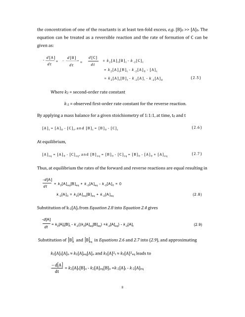
the concentration of one of the reactants is at least ten-fold excess, e.g. [B]0 >> [A]0. The
equation can be treated as a reversible reaction and the rate of formation of C can be
given as:
d [A ]
- = -
d t
d [B ]
d t
=
d [C ]
d t
= k 2 [A ] t [B ] t - k -2 [C ] t
Where k2 = second-order rate constant
= k 2 [A ] t [B ] t - k -2 [A ] 0 - [A ] t
= k 2 [A ] t [B ] t - k -2 [A ] t - k -2 [A ] 0
k-2 = observed first-order rate constant for the reverse reaction.
By applying a mass balance for a given stoichiometry of 1:1:1, at time, t0 and t
[A ] t = [A ] 0 - [C ] t , a n d [B ] t = [B ] 0 - [C ] t
At equilibrium,
[A ] e q = [A ] 0 - [C ] e q , a n d [B ] e q = [B ] 0 - [C ] e q = [B ] 0 - [A ] 0 + [A ] e q
8
(2 .5 )
(2 .6 )
(2 .7 )
Thus, at equilibrium the rates of the forward and reverse reactions are equal resulting in
-d[A ]
d t
= k 2 [A ] eq [B ] eq + k -2 [A ] eq - k -2 [A ] 0 = 0
k -2 [A ] 0 = k 2 [A ] eq [B ] eq + k -2 [A ] eq (2 .8 )
Substitution of k-2[A]t from Equation 2.8 into Equation 2.4 gives
-d[A]
dt = k 2 [A] t [B] t - k -2 {(k 2 [A] eq [B] eq ) +k -2 [A] eq } - k -2 [A] t (2.9)
Substitution of [ B ] t and [ B ] eq in Equations 2.6 and 2.7 into (2.9), and approximating
k2[A]t[A]o ≈ k2[A]eq[A]o and k2[A] 2 t ≈ k2[A] 2 eq leads to
− d
dt
[ A]
= k2[A]t[B]o - k2[A]eq[B]o +k-2[A]t - k-2[A]eq