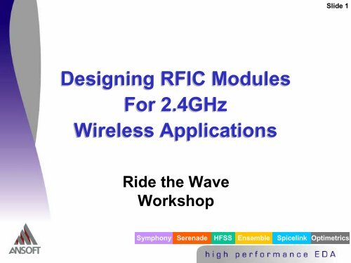
Designing RFIC Modules For 2.4ghz Wireless Applications

Designing RFIC Modules 

For 2.4GHz 

Wireless Applications 

Ride the Wave 

Workshop 

Slide 1 

Symphony Serenade HFSS Ensemble Spicelink 

Optimetrics

Agenda 

� Sample system: Bluetooth overview 

� System design and analysis 

� Antenna design and analysis 

� LTCC circuit design and analysis 

� RFIC design and analysis 

� Conclusion 

� References 

Slide 2

What is Bluetooth? 

Bluetooth [1] 

? [1] 

The Bluetooth system is is a universal radio interface on the 

globally available 2.4 GHz ISM frequency band facilitating 

wireless communication of of data and voice in in both stationary 

and mobile environments 

Low-cost Radio based cable replacement…(to)..Provide 

the basis for portable devices to communicate together 

…by creating a personal area (wireless) 

network…Bluetooth is an effort by a consortium of 

companies to design a royalty-free technology 

specification enabling this vision. (1) 

Low-cost Radio based cable replacement…(to)..Provide 

the basis for portable devices to communicate together 

…by creating a personal area (wireless) 

network…Bluetooth is an effort by a consortium of 

companies to design a royalty-free technology 

specification enabling this vision. (1) 

� Given the Bluetooth guidelines, how does this 

translate to RF specifications? 

Slide 3

Bluetooth Specifications Specifications [2] 

Specifications [2] 

� Operates in (U.S.) ISM band (2.400-2.4835 GHz) 

� Frequency hopping @1600 hops/sec(nominal) 

� Channel frequencies F = (2402+k) MHz, k = 0,…,78 

� Some countries use different ranges in this band 

� Channel spacing 1MHz 

� Guard band 2MHz lower, 3.5MHz upper. 

� Power classes: 

Power 

Class 

1 

2 

3 

Pmax 

100mW 

2.5mW 

1mW 

Nominal 

N/A 

1mW 

N/A 

Pmin 

1mW 

0.25mW 

N/A 

The Bluetooth 

system is is a narrow 

band system, 

approximately 3.5% 

bandwidth. 

Slide 4

Bluetooth Specifications 

� Modulation characteristic 

� 

� 

� 

GFSK with BT=0.5 

Modulation index : M I = 

Frequency deviation 

∆f( 

BW 

140 KHz ≤ 

∆f( 

SSB) ≤ 175KHz 

� Data rate : 1Mb/s 

2 SSB) 

0. 

28 

0. 

35 

(+/-160KHz nominal) 

� Radio frequency tolerance : +/-75KHz 

� Actual sensitivity level of -70dBm or better 

@0.1% raw bit error rate 

= 

~ 

Slide 5

Sensitivity and Dynamic Range [3] 

� Sensitivity 

� Minimum signal level that the system can detect with 

acceptable signal-to-noise ratio. 

Pin , min = − dBm / Hz 

� Dynamic range (SFDR) 

174 + NF + 10log 

B + SNR 

� Maximum input level that the circuit can tolerate to the 

minimum input level at which the circuit provides a 

reasonable signal quality. 

2P 

+ F 

3 

F = 

−174 

dBm + NF + 10log 

B 

IIP 3 

SFDR = − + 

( F SNR ) 

min 

min 

Slide 6

Bluetooth Noise Calculation [4] 

4.1 4.1 ACTUAL SENSITIVITY LEVEL 

The actual sensitivity level is is defined as as the the input 

level for for which a raw raw bit bit error rate rate (BER) of of 0.1% is is 

met. The The requirement for for a Bluetooth receiver is is an an 

actual sensitivity level of of –70 –70 dBm dBmor or better. The The 

receiver must achieve the the –70dBm sensitivity level 

with any any Bluetooth transmitter compliant to to the the 

transmitter specification specified in in Section 3 on on 

page 21. 21. 

This sets the noise budget for the system. The bit 

error rate, or P{E} for Non-coherent FSK is given 

by (2) 

This sets the noise budget for the system. The bit 

error rate, or P{E} for Non-coherent FSK is given 

by 

Where the approximation 

(2) 

1 Eb 

1⎛ 

S ⎞BT 

− 1 2 N 1 − ⎜ ⎟ 

0 

2⎝ 

N ⎠ k 

P{ 

E} 

= e = e 

2 

2 

Where the approximation 

is is used. 

E 

N 

b 

0 

⎛ S 

≈ ⎜ 

⎝ N 

⎞ 

⎟ 

⎠ 

BT 

k 

Bit Error Rate 

Bit Error Rate 

1.E+00 

1.E+00 

1.E-01 

1.E-01 

1.E-02 

1.E-02 

1.E-03 

1.E-03 

1.E-04 

1.E-04 

1.E-05 

1.E-05 

Bit Error Rate Vs. SNR, BT = .5 

Bit Error Rate Vs. SNR, BT = .5 

Non-coherent 

FSK 

Slide 7 

GFSK 

M 

I I =0.28 

1.E-06 

1.E-06 

-5 0 5 10 15 20 25 

-5 0 5 10 15 20 25 

SNR, dB 

SNR, dB 

Thus, the the signal to to 

noise ratio has has to to 

be be a minimum of of 

approximately 

21dB.

Bluetooth Noise Budget 

0 dBm 

-20 dBm 

-70 dBm 

-91 dBm 

-114 dBm 

TX power 

RX power @ 10cm 

RX power @ 10m, Reference Sensitivity Level 

Allotted Noise floor 

kTB (@1MHz) 

The ratio of of signal to to noise 

for for non-coherent GFSK 

was calculated to to be be a 

minimum of of 21dB for for the 

given BER specification. 

This allows a system 

noise figure of of 23dB. 

C/I AWGN = 21 dB 

(Theoretical) 

NF = 23 dB 

Slide 8

Bluetooth Intercept Point 

4.4 4.4 INTERMODULATION CHARACTERISTICS 

The reference sensitivity performance, BER = 0.1%, shall be be met met under the the following conditions. 

••The The wanted signal at at frequency ff 0 

0 with a power level 6 dB dB over the the reference sensitivity level. 

(Reference Sensitivity Level = -70dBm, signal @f @f 

0 

0 therefore is is –64dbm) 

•• A static sine wave signal at at f1 f1 with a power level of of –39 –39 dBm 

•• A Bluetooth modulated signal at at f2 f2 with a power level of of -39 -39 dBm Such that that ff 0 

0 = 2 ff 1 

1-f -f 

2 

2and and | | ff 2 

2-f -f 

1 

1 |= |= n*1 n*1 

MHz, where n can can be be 3, 3, 4, 4, or or 5. 5. The system must fulfill one one of of the the three alternatives. 

(f (f 

0 

0is is some desired signal, and and ff 1 

1 & ff 2 

2are are two two signals in in adjacent channels, as as evidenced by by the the restriction 

|f |f 

2 

2 –f –f 

1| 1| = n*1) 

This essentially sets the the dynamic range of of the the system by by 

setting the the intercept point through the the use use of of co-channel 

interference. In In this this case, the the third order product produced 

from signals in in two two adjacent channels are are at at the the same 

frequency as as the the desired signal. This third order product 

cannot cause a degradation in in BER. Since the the power in in the the 

“desired” channel is is –64dBm, the the third order product caused 

by by 2 ff 1 

1-f -f 

2 

2 (= (= f0) f0) has has to to be be below the the level specified for for 

Carrier Interference (C/I). The The C/I C/I specification is is 11dB, so so 

this this means that that the the third order product of of the the two two signals 

must be be below –75dBm. 

Output Power, dBm dBm 

Dynamic Range Chart 

50 

50 

40 

40 

30 

30 

20 

20 

10 

10 

0 

-10 

-10 

-20 

-20 

-30 

-30 

-40 

-40 

-50 

-50 

-60 

-60 

-70 

-70 

-80 

-80 

-90 

-90 

-100 

-100 

-110 

-110 

-120 

-120 

Ideal Power Output 

Ideal 

Ideal 

Power 

3rd Order 

Output 

Power Output 

Ideal Nois 3rd e Floor Order at Input Power Bandwidth Output 

Nois 

Compression 

e Floor at Input Bandwidth 

Compression 

Po, Spur-Free 

Po, 

System 

Spur-Free 

Noise Floor 

System Noise Floor 

-120 

-120 

-110 

-110 

-100 

-100 

-90 

-90 

-80 

-80 

-70 

-70 

-60 

-60 

-50 

-50 

-40 

-40 

-30 

-30 

-20 

-20 

-10 

-10 

0 

Input 

Input 

Power, 

Power, 

dBm 

dBm 

Slide 9

Output Power, dBm 

Bluetooth Intercept Point Calculations 


50 

40 

30 

20 

10 

0 

-10 

-20 

-30 

-40 

-50 

-60 

-70 

-80 

-90 

-100 

-110 

-120 

Ideal Power Output 

Ideal 3rd 3rd Order Power Output 

Noise Floor at at Input Bandwidth 

Compression 

Po, Po, Spur-Free 


-120 -110 -100 -90 -80 -70 -60 -50 -40 -30 -20 -10 0 

Input Power, dBm 

Noise Floor = kTB 

Slide 10 

Pin Vs Pout, Fundamental 

Estimated Compression 

Curve 

Output power level 

Corresponding to the point 

where the third order 

product meets the noise 

floor 

Pin Vs Pout, Third Order 


G + NF +kTB


40 40 

Minimum 

30 30 power point where 

the system must not produce 

a spur 20 20 higher than the (C/I), 

Output power = -39dBm + G 

10 10 

0 

-10 -10 

-20 -20 

-30 -30 

-40 -40 

Bluetooth TOI Calculation 

Third Order Intercept 


-50 -50 

-110 -110 -100 -100 -90 -90 -80 -80 -70 -70 -60 -60 -50 -50 -40 -40 -30 -30 -20 -20 -10 -10 


X 

2X 

Point where the third order product intercepts the 

noise floor, in this case the C/I ratio, 

Output power= –64dBm – 11dB + G = -75dBm + G 

X 

-39dBm 

-64dBm 

G 

-39dBm + G 

-64dBm + G 

Slide 11 

It It is is convenient to to refer refer to to the the both both the the output output and and 

the the input input of of the the device device when when calculating Third Third Order Order 

Intercept, even even though though the the gain gain will will drop drop out out for for 

input inputpoint. point. The The given given specification is is the the point point 

where where the the third third order order product is is equal equal to to the the “noise” “noise” 

level levelor or in in this this case, case, Carrier Carrier to to interference Ratio Ratio 

(C/I). (C/I). Once Once this this level level is is known, the the third third order order 

intercept can can be be calculated for for a given given gain. gain. The The 

slope slope of of the the fundamental is is 1, 1, and and the the slope slope of of the the 

third third order order product is is 3, 3, so so P 

out 

out Vs. Vs. P 

in 

inplot plot can can be be 

broken broken up up into into 2 regions regionsas as shown. shown. The The two two points points 

on on the the plot plot are are given given for for the the upper upper and and lower lower limits limits 

of of the the 2X 2X interval, or or at at the the output output 

2X= 2X= -75 -75 +G +G –(-39 –(-39 +G) +G) = 36, 36, X = 18 18 

And And the the Third Third order order intercept is is X dB dB above above –39dBm 

at at the the input, input, or or 

TOI TOI = -39dBm + 18dB 18dB = -21dBm 

Note Note that that the the input input intercept point point does does not not depend 

on on the the gain gain directly. 

Third Order Product 

-39dBm + G – 2X

Slide 12 

Bluetooth Spur Free Dynamic Range Calculations 


40 40 

Minimum 

30 30 power point where the 

system must not produce a spur 

higher 20 20 than the noise floor, 

Output power = -39dBm + G 

10 10 

0 

-10 -10 

-20 -20 

-30 -30 

-40 -40 


-50 -50 

-110 -110 -100 -100 -90 -90 -80 -80 -70 -70 -60 -60 -50 -50 -40 -40 -30 -30 -20 -20 -10 -10 


Y 

2Y 


Y 

As As before, the the dynamic range spur chart is is 

plotted. In In this this case, the the point of of interest is is 

the the point where the the output power third order 

product is is equal to to the the noise power. This is is 

the the lower end end of of the the SFDR. The The upper end end 

will will be be the the output power of of the the first first order 

product at at that that point. In In this this case, the the SFDR 

is is just just 2Y. 2Y. The The distance 3Y 3Y is is given by by 

3Y 3Y =-21+G -( -( -114+G+23 ) ) 

2Y=(2/3) (-21 +114 --23 23 )=46.7dB 

This difference is the Spur-Free Dynamic Range. 

The assumed noise figure was 23dB. 

Point where the third order product 

intercepts the noise floor, 

Output power = ktB+G+NF = -114dBm + G+23

Ansoft Design Environment for Wireless Design 

�� Ansoft design environment addresses the 

needs of the wireless market 

� Modern wireless systems are becoming more and 

more complex 

� Levels of integration are increasing 

� Time to market requirements are shrinking 

� Fast, accurate simulation is required 

�� Ansoft design environment provides start to 

finish design and analysis 

� Circuit simulation 

� System simulation 

� 2.5D modeling 

� 3D modeling 

� The following presentation demonstrates 

Ansoft’s answers to wireless design 

Slide 13

System Design and Analysis 

� Architecture considerations 

� System Architecture 

� GFSK modulation 

Slide 14 

� PLL Frequency Synthesizer design and analysis 


Optimetrics

Receiver Architectures 

� SuperHeterodyne receiver 

� Uses “dual” down-conversion 

� RF and LO are separated in frequency 

Slide 15 

� “Image” and other unwanted signals can be filtered (Cost) 

� More complex structure 

� Low-IF Heterodyne receiver 

� High level integration 

� Down-converts directly to a “low” IF 

� Image noise is a concern, medium channel selectivity 

� Direct Conversion(Zero-IF Homodyne) receiver 

� LO and RF at the “same” frequency 

� High level integration, no image filter 

� LO leakage is “in-band”, higher design challenge

Transmitter Architectures 

Transmitter 

Transmitter Architectures [5] 

� Direct VCO modulation 

� Direct VCO modulation with gaussian filtered data 

� Simple, low current design 

� Frequency drift and modulation index variation 

� I/Q modulation 

� Direct or indirect up-conversion with I/Q modulator 

� Gaussian filter and FSK mapping are performed in BB 

� No frequency drift 

� No modulation index variation 

� More circuits are involved 

Slide 16

Symphony 

System Architecture 

Slide 17

Signal Implications 

� GFSK Modulation 

� Gaussian Frequency Shift Keying 

� The information is contained in the “frequency shift” of 

the signal between two frequencies. 

� BT = .5 

� B bandwidth of the gaussian filter used, in this case .5MHz 

LPF, corresponds to a 1MHz bw at 2.4ghz. 

� Since there is one bit/symbol, T is the bit time and the 

Symbol time. 1/T is the bit rate. 

� The goal of Bluetooth is to have a data rate of 1Mb/s 

� GFSK is ideally a constant envelope signal 

� This implies a “constant amplitude” signal 

� Power amplifier can be run deep into compression 

� This increases the efficiency of the power amplifier 

Slide 18

Gaussian Frequency Shift Keying (GFSK) [6] 

In a GFSK modulator everything is is the same as a FSK 

modulator except that before the baseband pulses (-1, 1) go 

into the FSK modulator, it it is is passed through a gaussian filter 

to make the pulse smoother so to limit its spectral width. 

Gaussian filtering is is one of the standard methods for 

reducing the spectral width or Pulse Shaping. If If we use “-1” 

for fc-fd and “1” for fc+fd, when we jump from -1 to 1 or 1 to - 

1, the modulated waveform changes rapidly, which 

introduces a large out-of-band spectrum. If If we change the 

pulse going from -1 to 1 as -1, -.98, -.93 ..... .96, .99, 1, and 

we use this smoother pulse to modulate the carrier, the outof-band 

spectrum will be reduced. 

The spectral width for FSK is is unlimited, comparatively, there 

is is a limitation on GFSK. fc "climbs slowly" to fd in GFSK, 

However, in the case of FSK, fc "jumps sharply" to fd, which 

greatly decreases spectral efficiency.. 

Slide 19

Frequency Shift Keying (FSK) Vs. 

Gaussian Frequency Shift Keying (GFSK) 

FSK Modulation 

GFSK Modulation 

Symphony 

Addition of Gaussian 

Low Pass Filter 

Slide 20

Symphony 



FSK GFSK 

Slide 21

Symphony 



Slide 22

Symphony 



Slide 23

Forward gain: 

B( 

s) 

PLL Frequency Synthesizer 

θ i( 

s) 

K K θo( 

s) 

θ 

0 

F(s) 

f i 

G( 

s) 

= 

K 

θ 

s 

K0F( 

s) 

s 

Open loop Transfer Function: 

Closed loop Transfer Function: 

1 

N 

s 

f o =Nf i 

Slide 24 

Kθ : Phase detector gain factor (Volts/Radian) 

K0 : VCO gain factor (Radians per second/volt) 

F(s): Filter transfer function 

N: Frequency Division Ratio 

H( 

s) 

K0F( 

s) 

Ns 

FowardGain G( 

s) 

KθK 

0F( 

s) 

s 

= 

= 

= 

1− 

( OpenLoopGain) 

1+ 

G( 

s) 

H( 

s) 

1+ 

K K F( 

s) 

Ns 

= 

K 

θ 

θ 

0

PLL Design Specs 

� Output frequency : 2402MHz~2480MHz 

� Frequency step : 1MHz 

� Lock-up time : < 220 µS 

� Overshoot : < 20% 

� VCO sensitivity : 40MHz/V (K o) 

� Reference Frequency : 1MHz 

Slide 25

Setting Time Calculation for PLL 

625X5 = 3125us 

2871 bits 

Standard packet format: 

LSB 72 54 0 ~ 2745 MSB 

ACCESS CODE HEADER PAYLOAD 

Symbol Rate = 1Ms/s = 1Mbps → Bit Duration 

= 

1µ 

s 

∴Max 

number of bits of a standard packet is 72 + 54 + 2745 = 2871 

Therefore, the time left for 3 slot times and settling is (3125-2871) = 254 µsec 

∴ 

1 

1600 hops 

625 s = 

µ 

/ sec 

Slide 26 

for 5 time slots

Setting Time Calculation for PLL 

Hopping 

Turn around 

If the hop sequence scans over the turn around region like segment1 & segment2, PLL in radio chip should 

be capable of switching and settling (for all of the frequency hop) before the onset point of next time slot. 

Assume 3-wire control takes about 34us (based on 13MHz system clock), then 

1. Channel switching time should be < 220us 

2. Tx-Rx turn around time should be < 220us for the frequency jump of 78MHz. 

Slide 27

Error 

100 

80 

60 

40 

20 

0 

-20 

-40 

-60 

Setting Time & Loop Bandwidth for PLL 

e 

Error vs Time 

tζ 

T 

o 

= 

ωo 

t⋅ζ 

⋅ 

2π 

0 50 100 150 200 

Time 

e 

It should be 

Dimensionless here!! 

if 

e 

ωo 

−t⋅ζ 

⋅ 

2π 

≤ 

Slide 28 

Set as 

⎯⎯→ 

⎯ ε 

ωo 

⇒ t ⋅ζ 

⋅ ≥ −lnε 

2π 

ωo 

When t = ts 

⇒ ts 

⋅ζ 

⋅ = −lnε 

2π 

− lnε 

ωo 

= 2π 

⋅ 

t ⋅ζ 

s 

f 

f 

accuracy 

jump( max ) 

RADIO FREQUENCY TOLERANCE 

The transmitted initial center frequency accuracy must be ±75 kHz from F c . The initial frequency 

accuracy is defined as being the frequency accuracy before any information is transmitted. Note 

that the frequency drift requirements not included in the ±75 kHz. 

Θ 

f 

Θ t 

s 

accuracy 

= 75KHz, 

= 220µ 

s & let ζ = 

f 

jump(max) 

0. 

8, 

∴ 

= 78MHz 

f 

o 

= 

− lnε 

≅ 

t ⋅ζ 

s 

∴− 

lnε 

≈ 

6. 

947 

39. 

47KHz, 

whereω 

= 

0 

2π 

⋅ 

f 

0

Serenade 

2 1 sτ 

+ 

F( 

s) 

= 

s 

F( 

s) 

[ ( τ + τ ) ] 

1 

1 sτ 

+ 

2 

Loop Filters 

τ = R C 

τ 

1 

2 

= 

1 

R 

2 

2 

C 

τ = R C 

1 

τ 

= 

1 

R 

2 

C 

2 

F( 

s) 

= 

[ s( 

τ + τ ) + 1]( 

sτ 

+ 1) 

F( 

s) 

= 

sτ 

+ 1 

Slide 29 

2 

2 2 2 2 

= 

sτ 

sτ1( 

sτ 

3 + 1) 

1 

1 

sτ 

+ 1 

2 

2 

τ1 

= R1C2 

τ = R C 

2 

3 

2 

2 

( R1 

R2 

) 3 

τ 3 = || C

Closed Loop Bandwidth Response 

Symphony 

Serenade 

Slide 30

Closed Loop Bandwidth Response 

Symphony 

Serenade 

35KHz 

Slide 31

Tx-Rx Tx Rx Turn Around & Channel Switching Time 

Symphony 

Serenade 

80MHz Frequency Jump 

10MHz Frequency Jump 

Slide 32

Spur Simulation for PLL 

• Open loop modulation when transmitting (Turn off phase detector after loop is locked, no spur problem) 

• Close loop for PLL when receiving (The receiver will suffer from comparing spur interferences from PLL) 

Symphony 

R 

out 

(to emulate the curent leakage) 

= 

Settling Voltage 

Leakage Current 

Slide 33 

1v 

5 

≈ = 5⋅10 

Ω 

2µ 

A

The case for 

in1 lag in2 

Symphony 

Phase Frequency Detector 

The case for in1 lead in2 

Slide 34

Interference 

(On purpose) 

Symphony 


??? 

Interference 

(generated by PLL when receiving) 

Slide 35

If finterference≥3MHz 

If finterference=2MHz 

If finterference=1MHz 

40dB 

30dB 


-67 

dBm 

-60 

dBm 

-60 

dBm 

-27dBm 

-30dBm 

-67dBm 

X dBc 

X dBc 

X dBc 

Slide 36 

- 67dBm - (-27dBm + X) ≥ 11dB ⇒ X ≤ −51dBc 

The tightest spec. for PLL 

comparing spur suppression!! 

- 60dBm - (-30dBm + X) ≥ 11dB ⇒ X ≤ −41dBc 

- 60dBm - (-60dBm + X) ≥ 11dB ⇒ X ≤ −11dBc

Antenna Design 

� Antenna in a Bluetooth-enabled 

device is a vital part of the whole 

solution 

� Product power consumption 

� BER 

� Inverted-F antenna 

� Allows for embedded design 

� Low-profile and small (~λ/4) 

� Inductive tuning stub 

� Good BW and gain due to use of board 

ground plane 

HFSS Ensemble 

Optimetrics 

Slide 37

� Typical PDA board 

size(100mmx60mm) 

Model and Results 

� 3D-modeling with HFSS 

� Finite ground and dielectrics 

simulated 

� Gap source used 

� PML (Perfectly Matched 

Layer) absorbing boundary 

condition used 

� -14dB at 2.44GHz 

� BW > 0.8GHz 

� VSWR < 2 over entire band 

HFSS 

Slide 38

z 

x y 

HFSS 

Radiation Patterns 

Slide 39

LTCC Circuit Design and Analysis 

� Tx & Rx Baluns 

� Power Amplifier mounted on 

substrate 

Slide 40

RF Module for bluetooth [7] 

� Size requirements of RFIC require flip-chip assembly 

� LTCC selected for high frequency performance and 

dense integration of antenna filter and Rx/Tx baluns 

� Single-side assembly allows for one soldering 

operation. 

� Package is self-shielding due to ground plane in 

substrate and BGA balls. 

Slide 41

What is LTCC? [8] 

� Low Temperature Co-fired Ceramic (LTCC) 

technology meets the requirements for MCM-C 

design 

� Benefits/Features of LTCC 

• Hi Q/ Low Loss / Low T 

• Allows direct attachment 

of Si and GaAs IC’s 

• Ag & Au based conductors 

• Enhances performance, 

decreases cost, reduces size 

and improves reliability 

Slide 42

� 8-layer LTCC 951 Green Tape TM by DuPont 

� parallel processing 

� excellent dielectric isolation 

� high layer count circuitry 

� high conductivity metallization 

� 951A2 properties: 

LTCC 

• Layer thickness (fired) = 0.1397mm 

• Dielectric constant = 7.8 

• Loss Tangent = 0.0015 

• Metal type = Silver (Ag) 

Slide 43

Balun Model on LTCC 

Rx and Tx baluns 

LTCC 

Substrate 

PCB 

Serenade HFSS Ensemble Spicelink 

Optimetrics 

balun layers 

g2 

stripline: routing 

g1 

microstrip: soldering and interconnects 

RFIC 

Slide 44

Baluns 

� Baluns provide a “balanced” output from a 

single input 

� Outputs are 180º out of phase 

� Ports are “isolated” 

� Baluns are difficult to simulate 

� “Conductive” silicon substrate 

� Multiple layers 

� Ensemble can simulate the structures on 

both LTCC and for “on chip” applications 

using a 2.5D approach 

� HFSS Can be used to provide a full 3D 

simulation 

Slide 45

Baluns 

� Baluns can be realized with either 

active or passive components 

� Active baluns require additional DC 

current 

� Passive Baluns are typically bulky 

and difficult to realize 

� Passive Baluns can be located on-chip 

or “off chip” 

Slide 46

Balun configurations 

1. 180° hybrids / ring resonators – 

impractical due to large size 

2. Lumped-element filter type – poor 

balance and complicated layout 

3. Marchand type – excellent balance over 

wide frequency band 

� Coupled microstrip, Lange-coupler: 

� large geometry 

� Spiral type: 

� compact layout due to 

geometry and mutual coupling 

� lower series resistance due to less metal 

Slide 47

Balun layout [9] 

� Upper conducter centered 

above gap in the lower 

conducter and rotated 180°. 

� Allows for independent variation of center-to-center 

spacing (mutual L) and overlaid degree (mutual C). 

� Forces close to coplanar structure (Zo nearly 

independent of substrate thickness). 

� Direction of current flow in coils is same (better 

mutual L). 

� Layout symmetric to ground connections (minimized 

imbalance). 

� Coplanar ground ring provides shielding 

� fo of balun tuned by changing 

N or Rinner . 

� Optimal performance when 

W/(W+S) = 0.4~0.6. 

Slide 48

Balun stackup 

� M2, M4, M8 : solid ground layers 

Slide 49 

� M3 : stripline layer used for routing between 

embedded components, discrete components and 

board 

� M5, M6, M7 : balun layers 

� Dielectric thickness = 0.1397mm per layer 

� Metallization thickness = 0.009mm 

M8 

M7 

M6 

M5 

M4 

M3 

M2

Baluns coil size approximation 

� Required 90° length derived from 

transmission line utility in Power 

Plug-Ins 

� L = 10.99mm 

� Physically, 

L 

Ri 

+ W + S 2 2 

( θ , θ , R , W , S) 

= R ( θ −θ 

) + ( θ −θ 

) 

1 

2 

i 

i 

2 

1 

� Single coil modeled initially to get 

close to 90° phase lag, where: 

� W=S=0.15mm 

� R i =0.15mm 

� N=2.5→ θ 1=0°, θ 2=90° 

4π 

0. 

45 

L 19 

4π 

2 ( 0, 

5π 

, 0. 

15, 

0. 

15, 

0. 

15) 

= 0. 

15( 

5π 

) + ( 5π 

) = 11. 

mm 

� L=11.19mm →φ=91.63° in TRL utility, 

which is close enough to start. 

Serenade 

2 

1 

Slide 50

� Gap sources on 

input and output of 

both coils. 

� Solid coplanar 

ground ring used to 

reduce model 

complexity in initial 

design. 

∠ 

� d 

S 

∠S 

21 

43 

ο 

( 2. 

44Ghz) 

= 97. 

7 

ο 

( 2. 

44Ghz) 

= 90. 

5 

� Absolute phase and 

phase imbalance 

addressed during 

optimization. 

HFSS Optimetrics 

Single coil model 

port3 

port1 

port2 

port4 

Slide 51

Full 3-port 3 port model 

� Coil mirrored around z-axis to generate baluns. 

� Ground provided by solid coplanar ring, and top and bottom of 

bounding box. 

� Model creation programmed in macro language to allow for 

parametric analysis on W, S, Ri, and N. 


port3 

open 

port1 

port2 

Slide 52

Balun analysis and performance 

� Solution space defined as: 

� Ro=[0.15, 0.55] mm 

� S=[0.15, 0.55] mm 

� W=[0.15, 0.55] mm 

� N=2.5 

� IL, phase imbalance, and amplitude imbalance calculated 

within Optimetrics: 

2 2 

( ) 

2 2 ⎛ S12 

S13 

2 S12 

S13 

cos ⎞ 

IL 10log 

S12 

S13 

10log⎜ 

+ + 

θ 

= − + − 

⎟ 

2 2 

⎜ S12 

S13 

2 S12 

S ⎟ 

⎝ + + 13 ⎠ 

≈ −10log 

S 

2 

+ S 

2 

( ) 

12 

13 

phase imbalance = 180° 

− tan 

−1 

⎛ S 

Im⎜ 

⎝ S 

⎛ S 

Re⎜ 

⎝ S 

12 

13 

12 

13 

⎞ 

⎟ 

⎠ 

⎞ 

⎟ 

⎠ 

⎛ S 

amplitude 

imbalance = 20log 

⎜ 

⎝ S 

Slide 53 

12 

13 

⎞ 

⎟ 

⎠

Balun parametric sweep vs Ri 


•Ri=0.25; W=S=0.15 

•Low IL, AmpImb 

•PhsImb corrected in layout 

Slide 54


Parameters vs S 

Slide 55


Parameters vs W 

Slide 56

Detailed balun model 

� Optimal design chosen: 

� Ri=0.25mm; W=S=0.15mm 

� IL=0.122dB; AmpImb=0.217dB; PhsImb=171° 

� Solid ground ring replaced by coplanar 

ground rings on each layer. 

� Via transitions, through LTCC substrate, 

to stripline mode included. 


Slide 57

� AmpImb≈0.355dB 

� PhsImb≈174° 

� IL≈0.508dB 

� Imperfect phase 

balance compensated 

for in layout. 


Balun 1 Results 

Slide 58

Final balun results 

� AmpImb≈0.0897dB 

� PhsImb≈179° 

� IL≈0.476dB 

� Use this balun in circuit/system 

simulation 


0.774mm 

Slide 59

Power Amp Specs 

� Device: BFP450 (Infineon) 

� Frequency: 2400Mhz ~ 2483MHz 

� Gain: ~10dB 

� Max. output power: > 0dBm 

� Substrate: LTCC 

� ε r = 7.8 

� Dielectric thickness : 139 µm 

� Metal thickness : 8 µm 

Symphony Serenade Ensemble 

Slide 60

Power Amp Design Procedure 

� Optimize bias network 

� Check stability K 

� Design matching network using Smith Tool 

� Optimize the output power 

� Nyquist stability analysis 

� Single-tone HB analysis 

� Two-tone HB intermodulation analysis 

� Digital modulation analysis 

Symphony Serenade Ensemble 

Slide 61

Bias circuit 

Serenade 

Input matching 

SmithTool Utility 

Input stability 

Power gain Circle(L) 

SmithTool environment 

Power gain Circle(S) 

Output matching 

Slide 62 

Output(L) stability

Serenade 

Nyqiust Stability Analysis 

Slide 63

Actual Circuit and Layout 

Serenade S2A Layout 

Ensemble 

Input 

Bias 

Output 

Slide 64 

4.4×4.9 mm

Serenade 

Single-Tone Single Tone HB Analysis 

Lumped in blue 

Distributed in red 

Slide 65

Serenade 

Two-Tone Two Tone HB Analysis 

Slide 66

Serenade 


Slide 67

Digital Modulation (Spectrum) 

Serenade 

Slide 68

Serenade 

Digital Modulation (ACPR ) 

Slide 69

RFIC Design and Analysis 

� Spiral inductor design 

� Baluns on chip 

� LNA design 

� Mixer 

Slide 70 


Optimetrics

Spiral Inductors 

� High Q is very important for VCO 

Bluetooth design 

� stable resonance frequency 

� low phase noise 

� Physical models 

� inductor performance relative to model 

� model extraction methods 

� Design curve generation for IC design 

� High Performance Spirals 

� approaches to increase Q 

� Examples 

Slide 71

Physical Model of Spiral on Si [10], [11] 

� Ls: Spiral inductance. 

� Rs: Series metal resistance. Symbolizes 

energy lost due to skin effect and 

induced eddy current in conductive 

media close to inductor. 

� Cs: Capacitance due to overlaps 

between spiral and underpass. 

� Cox: Oxide capacitance between the 

spiral and substrate. 

� Csi: Silicon substrate capacitance. 

� Rsi: Silicon substrate resistance. 

Other Measures of Performance 

� Q: Quality factor = 2π (energy 

stored)/(energy loss in one oscillation 

cycle) 

� fo: Self resonance frequency. 

Slide 72

ωLs 

Q = ⋅ 

R 

R 

R 

p 

2 ( ωL 

R ) + 1) 

( C + C ) 

Inductor Performance 

ground Port 2 

⎡ Rs 

⋅ ⎢1 

− 

⎣ 

s 

Ls 

p 2 

−ω 

Ls 

( Cs 

⎤ 

+ C p ) ⎥ 

⎦ 

ωLs 

= ⋅ substrate _ loss _ factor ⋅ self _ resonance _ 

R 

s 

s 

p 

+ 

s 

s 

R 

s 

factor 

Slide 73

� W = width 

� S = spacing 

Square Spiral Model 

� N = number of turns 

� Ri = inner radius 

� Coplanar ground ring 

used 

� Zero_Order=1 

� “Solve in” metal 

� Skin-depth seeding 

� 2 nd order absorbing 

boundary condition 

used 

HFSS Ensemble 

Optimetrics 

Slide 74

generated using macro language 

high matrix convergence required 

for accurate Q calculation 

automatically calculated and 

exported to a serenade circuit 

random and gradient optimization 

used to match S-parameters. 

HFSS/Serenade co-optimization 

co optimization 

Serenade HFSS Optimetrics 

3D Model(S,W,Ri,N) 

HFSS Solve 

S, Y parameter 

Serenade Optimization 

Optimetrics 

Equivalent Circuit Extraction 

Cost(Q, fself, Ls) 

Slide 75 

Equivalent circuit parameters 

and derived quantities can be fed 

back into Optimetrics for physical 

optimization of the spiral inductor

Design curve generation using Optimetrics 

and Serenade 


Slide 76

High Performance Inductors 

� 2 approaches to increasing Q 

� Without alteration of fabrication process: 

� multilevel spirals – reduce Rs, reduce Csi 

� patterned ground shields – reduce Rsi, Csi 

� With alteration of fabrication process: 

� high conductivity metal layers: decrease Rs 

� multimetal layers: increase thickness to decrease Rs 

� low-loss substrates (SOI, SOS, HRS, glass): 

decrease Rsi 

� thick oxide layer: isolate inductor from Si to decrease 

Csi, Rsi 

� micromachining techniques: descrease Rsi, Csi 

Slide 77


Spiral Layout [12] 

� Symmetric spiral inductor design 

� Test fixture included in HFSS 

simulation 

Slide 78

Open Test Fixture Model 

� Spiral inductor removed for open standard 

simulation 

� Single shunt impedance assumed for test 

fixture error network 


Slide 79

Test-Fixture Test Fixture de-embedding 

de embedding 

� Fixture introduces parasitics in measurements (these can 

drastically reduce the observed Q in measurements) 

� Fixtures need to be characterized with an error model 

� Many error models and calibration procedures – 12-term 

error model, TRL, TSD, etc… 

error network A DUT error network B 

A B 

A’ B’ 

� Calibration procedures typically use multiple standards to 

advance measurement plane past fixture discontinuities: 

� Similar standards and de-embedding procedures can be 

used within when modeling and/or matching measurements 

Slide 80

Y-matrix matrix de-embedding 

de embedding 

� Simple error network assumption → not as 

accurate as other de-embedding procedures 

2-port: 

1-port: 

Y A 

DUT 

A A’ B’ 

B 

Y A 

DUT 

Y B 

A A’ B’ 

B 

Y B 

Y 

Y 

tot 

' 

tot 

Y 

Y 

= Y 

= Y 

tot 

' 

tot 

A 

tot 

= Y 

= Y 

+ Y 

−Y 

A 

tot 

DUT 

A 

+ Y 

Slide 81 

− Y 

+ Y 

−Y 

A 

B 

DUT 

B

Spiral Q-factor Q factor Results 

� Peak Q (post-deembedding) of 7.73 

� Calibration of test fixture changed Q by 3.03% 

� Self-resonant frequency increases due to 

removal of parasitic capacitances in fixture 


Slide 82

Modified Spiral Inductor 

� 100um Si removed from beneath spiral to 

increase Q 

air 


Slide 83

Spiral with Si etched Results 

� Peak Q (post-deembedding) of 10.51 

� Calibration of test fixture changed Q by 7.5% 

� 36% improvement in Q with etching 


Slide 84

� Gummel Poon 

� Materka 

� TOM3 

� BSIM3 

Serenade 

FET Modeling 

Slide 85

MOSFET Characteristics 

� 

� 250µm 250µm geometry 

� 

� 5µm 5µm gate gate length length 

� 

� .2µm .2µm gate gate width width 

Serenade 

Slide 86

Typical Baluns: Baluns: 

Active and Passive 

Slide 87

Typical Baluns: Baluns: 

Active and Passive 

Slide 88

Baluns Calculation 

� Set variables in Serenade for a generic 

hybrid 

1 

ωL 

= = 

ωC 

� Set R = 50Ω 

2R 

� Frequency = f = 2.4ghz 

C = 

ω 

1 

2R 

L = 2πf 

2R 

Slide 89

Serenade 

Passive Balun Example 

Slide 90

Serenade 

Passive Balun Loss 

Slide 91

Serenade 

Passive Balun Phase Match 

Slide 92

Serenade 

Active Balun Example 

Slide 93

Active Balun Output Voltage 

Serenade 

Slide 94

Active Balun Output Spectrum 

Serenade 

Slide 95

LNA 

� Lowest possible noise 

� Low power consumption 

� CMOS technology (.2µm Gate width) 

� Critical Parameters 

� Gain 

� Noise Figure 

� Third order intercept 

Slide 96

LNA Design Procedure 

� Choose Geometry such that 

1 

gm 

≈ 50Ω 

� Choose Topology 

� Cascode with Inductive Degeneration 

� Choose Ls Such That 

L 

S 

≈ 

50Ω 

2πf 

� Choose Lg to “match” Cgs 

t 

L g 

L s 

Slide 97

LNA Design 

� Gate Degeneration 

� (Series Feedback!) 

� Cascode Design 

� Better output match 

� Input noise match inductance 

� Ideal Circuitry 

Slide 98

Serenade 

LNA Ideal Schematic 

Slide 99

LNA Small Signal Performance 

Serenade 

Slide 100

LNA Large Signal Performance 

Fundamental 

Serenade 


Slide 101

Serenade 

LNA Third Order Intercept 

Slide 102

Serenade 

Modulation Spectrum 

Slide 103

Mixer Characteristics 

� Optimal LO power 

� Third Order Intercept Point 

� Conversion Loss (Gain) 

� Noise Figure 

� DC Power Consumption 

� Input Match 

� Spurious Response 

� Image Rejection 

Slide 104

An An LO LO signal is is applied to to the the gate of of a 

FET, which is is enough to to turn the the drain- 

Source channel “on” and and “off.” Even 

though the the LO LO signal is is sinusoidal in in 

nature, the the characteristics of of the the FET 

junction is is such that that the the channel is is 

“square wave” modulated. The FET 

acts as as a switch. 

LO 

-1 

-3 

-5 

FET Mixer Operation 

RF 

6 

3 

0 

-3 

-6 

Time Time domain representation 

of of Drain-Source Channel 

Time 

Slide 105 

RF Input. 

D-S Channel 

“modulation” 

or the results 

of the LO on 

the Gate 

Resultant 

Product of 

the two 

signals

LO 

In In the the frequency domain, the the 

signals on on the the FET can can be be 

represented as as shown. 

FET Mixer Operation 

RF 

Frequency domain representation 

of of Drain-Source Channel 

0.01 

0.1 0.2 0.02 0.3 

0.4 

0.5 

2.4 

2.41 

4.82 

7.23 

0.01 0.1 10 

0.1 1 10 

Frequency 

9.64 

Slide 106 

RF Input. 

D-S Channel 

“modulation” 

or the results 

of the LO on 

the Gate 

(partial) 

Resultant 

Product of the 

two signals 

(partial)

Rx Input 

From Balun 

Image Reject Mixer 

90º 

LO Input 

From PLL 

90º 

IF 

Output 

Slide 107

Mixer Topologies: Image Rejection 

For Baseband downconversion, 

signal and noise from the upper 

and lower “sidebands” will be 

converted to the IF. Some form 

of image rejection is necessary 

Typical “Homodyne” System 

For dual downconversion, this 

sideband can be filtered 

Requires 2 mixer functions and 

filtering 

RF u -LO 

LO - RF L 

RF u -LO 

LO - RF L 

Filter 

Typical “Heterodyne” System 

LO 

LO 

RF L 

LO 

LO 

RF L 

Slide 108 

RF U 

RF U

Mixer Phase 

� Mixer “IF” phase is the sum of the 

phases of each frequency component. 

� This is a relative phase and will be used 

for image rejection calculations. 

RF ∠ ∠ ∠ φ 

φ 

LO ∠ ∠ θ 

θ 

Other Components 

Frequency: mRF ± nLO 

Phase: mφ φ φ φ ± nθ 

Slide 109 

∠IF (= ∠LO – ∠RF) = = θ θ - φ 

φ

LO ∠ ∠ ∠ ∠ ∠ ∠ ∠ ∠ ∠ ∠ ∠ ∠ 0º 

Image Reject Mixer Operation 

LO ∠ ∠ 0º 

In Phase 

Divider 

LO ∠ ∠ 90º 

LO - RFL ∠ ∠ 0º 

RFU -LO ∠ ∠ 0º 

90° 90° 

RF U ∠ ∠ ∠ ∠ ∠ ∠ ∠ ∠ ∠ ∠ ∠ ∠ 0º 

RF L ∠ ∠ ∠ ∠ ∠ ∠ ∠ ∠ ∠ ∠ ∠ ∠ 0º 

LO - RFL ∠ ∠ 90º 

RFU -LO ∠ ∠ -90º Slide 110 

RFU -LO ∠ ∠ ∠ 0º 

RFU -LO ∠ ∠ 0º 

RF U - LO 

LO - RFL ∠ ∠ ∠ 0º 

LO - RFL ∠180º 

0 

RFU -LO ∠ ∠ 90º 

RFU - LO ∠ ∠ -90º 

0 

LO - RFL ∠ ∠ 90º 

LO - RFL ∠ ∠ 90º 

LO - RF L

Typically, RF buffer 

FETs would be placed 

at the source of the 

mixer FETS. 

Replacing these FETs 

with Resistors will allow 

a lower voltage 

operation, and provide 

self-bias and feedback 

to reduce the effects of 

device mismatch on RF 

and LO operation. [3] 

Gilbert Cell FET Mixer 

+ LO 

+ IF -IF 

+ RF 

-LO 

-RF 

Slide 111 

-LO

Serenade 

Gilbert Cell FET Mixer 

Slide 112

IF Output Power Vs. LO Power 

Serenade 

Slide 113

Serenade 

IF Output Spectrum 

Slide 114

Conversion Gain Vs. RF Input Power 

Serenade 

Slide 115

Large Signal Mixer Performance 

Fundamental 

Serenade 


Slide 116

Large Signal Mixer Performance 

Serenade 


Slide 117

Conclusion 

� A “typical” wireless system has been defined and 

explained 

� System level analyses have been performed 

using Symphony 

� System specifications have been broken down 

into component requirements 

� Passive and multi-layer structures have been 

analyzed using HFSS and Ensemble 

� Active circuitry has been designed and analyzed 

using Serenade 

� Solutions to wireless design problems 

have been addressed using Ansoft design 

environment 

Slide 118

Any Question? 

Slide 119

References 

1. Haarsten, Jaap C. “The Bluetooth Radio System” IEEE Personal 

Communications, Feb. 2000 

2. Specification of the Bluetooth System, Version 1.1, February, 2001 

3. Behzad Razavi, “RF Microelectronics”, Prentice Hall, pp48-50, 1998. 

4. Sklar, Bernard, “Digital Communications, Fundamentals and 

Applications,” 1988 

5. Marshall Wang, “Design Consideration for Low Cost Bluetooth 

Transceiver/Modem”, Bridging the Gap with Blutooth, IEEE MTT Santa 

Clara Valley Chapter Workshop, April, 2001. 

6. http://www.palowireless.com/infotooth/knowbase/radio/109.asp 

7. Arfwedson, Sneddon, “Ericsson’s Bluetooth Modules”, Ericsson Review 

No. 4, 1999. 

8. DuPont Green Tape Design and Layout Guideline, 

http://www.dupont.com/mcm/gtapesys/part1.html. 

9. Yoon, et al., “Design and Characterization of Multilayer Spiral 

Transmission-Line Baluns”, IEEE Trans. on Microwave Theory and 

Techniques, vol. 47, no. 9, September 1999, pp1841-1847. 

Slide 120

References 

10. Yue, “Physical Modeling of Spiral Inductors on Silicon”, IEEE Trans. on 

Electron Devices, vol.47, no. 3, March 2000, pp560-568. 

11. Yue, “On-Chip Spiral Inductors with Patterned Ground Shields for Si- 

Based RF IC’s”, IEEE Journal of Solid-State Circuits, vol. 33, no. 5, May 

1998, pp743-752 

12. Niknejad, “Analysis, Simulation, and Applications of Passive Devices on 

Conductive Substrates,” PhD Thesis, Univ. of California at Berkeley, 

Spring 2000 

Slide 121

Designing RFIC Modules For 2.4ghz Wireless Applications

Create successful ePaper yourself

Delete template?

Save as template?