APPLYING THERMOECONOMICS TO THE ANALYSIS OF ... - circe

Proceedings of ECOS 2009 22 nd International Conference on Efficiency, Cost, Optimization
Copyright © 2009 by ABCM Simulation and Environmental Impact of Energy Systems
August 31 – September 3, 2009, Foz do Iguaçu, Paraná, Brazil
APPLYING THERMOECONOMICS TO THE ANALYSIS OF THE NORTH
AMERICAN FOOD CHAIN
César Torres Cuadra, cesar.torres@endesa.es
Antonio Valero Capilla, valero@unizar.es
Alicia Valero Delgado, aliciavd@unizar.es
Maryori Díaz Ramírez, mdiaz@unizar.es
CIRCE – Centro de Investigación de Recursos y Consumos Energéticos
Centro Politécnico Superior University of Zaragoza, SPAIN
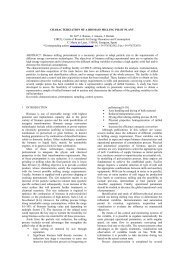
Abstract. Thermoeconomic analysis is used to understand the process of cost formation and how to improve the design
and the operation of extensive energy consumption systems such as power and chemical plants.
This paper shows the capabilities for using the thermoeconomic analysis in environmental systems, and demonstrates
that it could become a useful tool for identifying the ways for improving the energy resources cost and the efficiency of
a macroeconomic system such as the American food chain. The environmental impact associated to each process in the
food chain can be quantified through a thermoeconomic approach as a cost function, which represents the required
natural resources to obtain a final product. Symbolic exergoeconomics is used to quantify the environmental impact of
the food system. In the example, the fuel-product model is built and several simulations such as the impact of the
change of meat diet basis by a vegetable diet, and reusing the residual biomass are analyzed.
Keywords: Thermoeconomics, food chain, environmental systems.
1. INTRODUCTION
The earth is increasing naturally its entropy and the economic advance is accelerating the process because the
economic process degrades natural resources and pollutes the environment (Georgescu-Roegen, 1971).
Thermoeconomic analysis combines economic and thermodynamic analysis by applying the Second Law Analysis.
The physical entity connecting thermodynamics and economics is the entropy generation or irreversibility. It represents
the useful energy destroyed in all physical processes. Since all common processes in the actual industrial systems are
not reversible, natural resources are consumed and lost forever. The more irreversible a process is the more natural
resources are consumed. Nothing can be done without the expenditure of natural resources, and the amount of natural
resources required to obtain a “desired” product is equivalent to its thermodynamic cost. All the production processes
are irreversible. Consequently, the thermodynamic cost of a product can be also expressed as the “useful” energy
contained in the product plus all the irreversibilities generated to obtain it (Torres et al., 2008). The analysis of the cost
formation of processes is where physics best connects with economics.
Thermoeconomic analysis normally uses exergy as the measure of the usefulness of the energy contained in the
production flows. The exergy of a flow is the minimum amount of work required for its production, from the
environment reference, and it lets to formulate the equivalence between different matter and/or energy streams of an
energy system.
Thermoeconomics is a general theory for energy saving (Lozano et al. 1993), which has been commonly used in the
analysis of power or chemical plants, see for example the CGAM (Valero et al. 1992) or the TADEUS (Valero et al.,
2002) works.
The aim of this paper is to explain how thermoeconomics can be applied to a wider variety of energy and
environmental systems. To illustrate their capabilities we will use as an example the analysis of the North American
food chain.
The methodology presented here is closely related to the input/output analysis (ten Raa, 2005), the mathematical
principles are very similar, but in the Fuel-Product model, the Second Law is used in the analysis of the economic
processes. Furthermore, it could be also connected to Life Cycle Analysis in general and to exergetic lifeycle analysis in
particular (Cornelissen, 1997).
In the traditional societies before 20 th century the ratio between required energy in agriculture and provided energy
in form of food was 1:100, hence their products took mainly their energy from the solar radiation absorbed by plants.
However, nowadays modern agriculture requires much more energy than the calories we consume in form of food. For
example, for industrialized beef production using animal feed from overseas the ratio is 35:1, and it may reach extreme
values of 500:1 for winter greenhouse vegetables (von Weizsacker et al. 1998).
Besides the CO2 coming from the fossil fuel use, agriculture production increases the atmosphere’s carbon stock
through forest clearing and the release of soil carbon through crop growing. Food production also contributes to global
warming through the release of methane from livestock, crop and the burning of residuals (Deumling, D. et al., 2003).
887

Every human activity has an environmental impact, with the food system being an important (and mandatory)
human activity. There is a wide variation in environmental impact according to the type of food, and the method of
producing the food. An important feedback principle links the environment and food systems. The environment
influences the quality and capacity of food production, which in turn influences the environment. A degraded
environment may be less healthy for humans and other organisms, and also less able to produce the range and amount
of food that an environment in better condition could achieve (Riley, M., 2005). Each basic process that comprises the
food chain has an efficiency and a resources cost that could be evaluated by means of the thermoeconomic analysis,
allowing the identification of improving options.
2. THE FUEL –PRODUCT MODEL
Symbolic Exergoeconomics (Torres, 2004) provides general relationships between the production demand and the
resources cost with the efficiency and irreversibilities of the individual process of an energy system. It is based on the
productive structure of the system and is represented by the fuel – product table, (fig. 1) which describes how the
production processes are related.
F0 F1 … Fn
P0 E01 … E0n
P1 E10 E11 … E1n
… … … Eij …
Pn En0 E1n … Enn
Figure 1. Generic Fuel-Product Table
In this table, the useful energy carried from the i-th process to the j-th process is represented as E ij . The sum of each
row of the table is the production of each process, and the sum of each column is the resources or fuel required for each
process.
Symbolic exergoeconomic provides two different representations of the productive model:
The FP representation allows relating the production and the cost of each process of the system as a function of:
F ≡ E , … E
• The external resources ( )
e 10 n0
• The efficiency of each process, represented by K D , a diagonal matrix whose elements are the unit
•
consumption of each process: κi ≡ Fi / Pi
.
The distribution ratios, represented by FP , a matrix whose elements are defined as yij ≡ EjiPj. The production of each process is obtained as:
( ) 1
P =〈 P| Fe The total production demand is calculated as:
where 〈 P| = KD− −
FP (1)
t
P T = y0P F e
(2)
y ( , , ) is a vector that contains the distribution ratios related to the environment.
t
where 0 ≡ y01 … y0n
The production cost of each process is given by:
*
CP=〈 P | C0where *
〈 P | = ( UD−
−1
FP )
(3)
the vector C0 ≡ ( c01E01, …, c0nE0n) contains the cost of the external resources and c 0i represents its unitary cost. The
magnitude used to measure the external resources determines the type of cost obtained.
The other representation, called PF representation, allows expressing the resources and their costs as a function of:
• The production demand P s ≡ ( E10, …,
En0)
• The efficiency of each process i i / i F P ≡ ε
• The junction ratios, represented by PF , a matriz which elements are defined as qij ≡ Eij/ Fi
The resources used in each process are obtained as:
( ) 1
F = F Pswhere 〈 F | = HD−
−
PF (4)
−1
and HD ≡ K D is a diagonal matrix (n× n), containing the efficiency ε i of each process.
The cost per production unit can be obtained as:
888

Proceedings of ECOS 2009 22 nd International Conference on Efficiency, Cost, Optimization
Copyright © 2009 by ABCM Simulation and Environmental Impact of Energy Systems
August 31 – September 3, 2009, Foz do Iguaçu, Paraná, Brazil
t
P
where cˆ0i ≡ c0iq0, i.
The total cost of the external resources 0
c = F c ˆ
(5)
0
0
C can be expressed as a function of the system demand as:
t
C = cˆ F P (6)
Using these relationships is it also possible to determine the variation of the total resources as a function of the
variation of the parameters of the PF representation:
n ⎛ ⎞
Δ C0 = ∑⎜c0iΔ q0 iFi + ∑ cP, jΔ qjiFi + cF, iΔ
κiPi
+ cP, iΔEi0⎟ (7)
i=
1 ⎝ j
⎠
The above expression is known as the Fuel Impact Formulae (Torres et al., 2002), the first two terms correspond to
the variation of the junction (structural) ratios, the third term to the variation of the processes efficiency and the last
term to the system demand variation.
Through the example presented in the next section, we will show how thermoeconomics can be applied to a
macroeconomic system such as the American food chain, giving insights on improving options.
3. APPLYING THERMOECONOMICS TO THE ANALYSIS OF THE FOOD CHAIN
The Global 2000 Report (Barney, 1980) presented a flow diagram of energy for American food production (see
figure 2). For around 3.6 GJ (per capita) of human food energy, 35.5 GJ of technical energy are expended, without
accounting for the “solar gift” of 80 GJ that is absorbed by the plants used in the process. It seems more than plausible
that the energy demand from agriculture and food processing could be substantially reduced with essentially no
sacrifice of wellbeing (Weizsacker, 1997). And thermoeconomics could help to identify and quantify these reductions.
According to the diagram of figure 2, the food chain system could be decomposed into five basic processes,
represented in the productive diagram of figure 3.
80 60
1 2
(1) Vegetal biomass production
(2) Harvest production
(3) Animal food production
(4) Vegetal food production
(5) Human food demand
7
0
51.5
5
3.5
s
15
3
4
13.5
Figure 3. Productive diagram of the food chain in the USA
3.1. The base food chain
The thermoeconomic model of the base food chain of Fig. 3 is represented by the following Fuel-Product table.
From this table it is possible to obtain the production cost of each process. In this example we are interested to separate
the cost associated to fossil fuels and the cost associated to biomass energy, because the saving of these resources has a
different interpretation. Fossil fuels are required in all processes of food production: draining, irrigation, chemical
products, mechanical manufacturing, cattle raising, food preparation, shipping and distribution…, whereas biomass
energy is provided by the plants, taking energy from the sun.
889
1.9
3.1
5
3.6

Table 1. Fuel-Product Table of the food chain (GJ)
0 F 1 F 2 F 3 F 4
F 5
F Total
P0 80 7 15 13.5 0 115.5
P1 0 0 60 0 0 0 60
P2 5 0 0 51.5 3.5 0 60
P3 0 0 0 0 0 1.9 1.9
P4 0 0 0 0 0 3.1 3.1
P5 3.6 0 0 0 0 0 3.6
Total 8.6 80 67 66.5 17 5
Equations (3) and (5) allow computing the production cost. These equations could be also used to decompose the
costs considering the different types of resources. The resource cost vector can be separated into two parts:
fossil biomass
fossil
C0 = C0 + C 0 , where the cost due to fossil fuels in terms of energy resources is C 0 = (0, E02, E03, E04,0)
, and
biomass
the cost due to biomass is C 0 = ( E01,0,0,0,0)
, therefore the production cost due to fossil fuel could be computed as:
fossil
CP= *
P
fossil
C0
(8)
and in the same way the production cost due to biomass is:
biomass
CP= *
P
biomass
C0
(9)
Similar expressions could be used to compute the unitary production cost.
Table 2. Efficiency and production costs of the processes for the base case
Fossil Fuels Biomass Total
Process κ P c (GJ/GJ) P C (GJ) P c (GJ/GJ) P C (GJ) P c (GJ/GJ) C P (GJ)
1 1.33 0.00 0.00 1.33 80.00 1.33 80.00
2 1.12 0.12 7.00 1.33 80.00 1.45 87.00
3 35.00 11.06 21.01 36.14 68.67 47.20 89.68
4 5.48 4.49 13.91 1.51 4.67 5.99 18.58
5 1.39 9.70 34.92 20.37 73.33 30.07 108.25
Total 13.43 35.50 80.00 115.50
In table 2 the efficiency values of each system process are shown. The ratio of the total fossil fuel required per
fossil
calorie consumed is approximately 10:1 ( c P,5
= 9.70 ), a clear indicator of the high inefficiency of the current food
chain. Also note that the production of meat (process 3) requires 2.5 times more fossil energy resources (11.06 vs. 4.49)
than the vegetal production (process 4). By far, the most inefficient process (identified by κ ) is the production of meat.
Starting with the base case we will analyze several scenarios, in order to demonstrate the capabilities of the
thermoeconomic approach for the evaluation of the environmental impact of the food system, and for the identification
of potential improvements.
3.2 Recycling biomass residues
Our aim now is to identify and quantify possible optimization options of the food chain system. In the first scenario,
we are going to analyze the effect of recycling 10% of crop residues (2 GJ) and reusing them as fuel in the next process.
The unit consumption of the first process is reduced to κ 1 = 1.29 and the external resources of the second process to
C 02 = 5. We assume that the distribution ratios and the final demand of the system do not change.
Using Eqn. (3) it is possible to compute the production costs. Since biomass energy and the cost distribution matrix
*
P does not change, the production costs due to biomass do not change either.
890

Proceedings of ECOS 2009 22 nd International Conference on Efficiency, Cost, Optimization
Copyright © 2009 by ABCM Simulation and Environmental Impact of Energy Systems
August 31 – September 3, 2009, Foz do Iguaçu, Paraná, Brazil
Table 3. Production costs due to fossil fuel, recycling 10% biomass
Fossil Fuels
Process P c (GJ/GJ) C P (GJ)
1 0 0
2 0.08 5
3 10.15 19.29
4 4.45 13.79
5 9.19 33.08
Total 33.50
Table 3 shows the new costs due to fossil fuels. As it can be seen, recycling 10% of crop residues reduces the fuel
consumption by 2 GJ, or what is the same, the ratio between the fuel required and the energy consumption is reduced by
5.25%.
3.3. Process efficiency impact
In this scenario we will assume that the efficiency of each single process is increased by 10% without modifying
the final demand and the system structure (junction ratios). Eqn (7) is used for this purpose, with Δ κi
= 0.1.
The impact
in resources consumption is decomposed into the part coming from biomass and from fossil fuels (see table 4).
Table 4. Impact of resources consumption with a 10% increase on the process efficiency
Process 0 C Δ Fossil Fuels (GJ) 0 C Δ Biomass (GJ) 0 C
Δ Total (GJ)
1 0.000 0.00% 6.000 7.50% 6.000 5.19%
2 0.627 1.77% 7.881 9.85% 8.507 7.37%
3 0.060 0.17% 0.216 0.27% 0.276 0.24%
4 0.254 0.71% 0.094 0.12% 0.347 0.30%
5 2.514 7.08% 5.808 7.26% 8.322 7.21%
Eqn. (10) is used to compute the fuel impact of each efficiency simulation. The cost of fuel is evaluated for the
simulated scenario and the production corresponds to the base case.
i
0
Δ C0 = cF, iΔ κi
Pi
(10)
Note that improving the efficiency of the last stage of the food chain has an important impact on the fossil fuel
consumption. On the other hand improving the efficiency of the first stages of the process has an impact only on the
reduction of biomass requirements. An important conclusion can be thus drawn: for improving the energy efficiency of
the food chain, major efforts should be focused on the last production stages.
3.4. Change in the food diet
The last scenario analyzes a change in the diet. As it has been shown, the production of animal food requires much
more resources than vegetable food. In the base model a person consumes 62% of vegetables and 38% of animal food.
What would happen if we reduced the consumption of meat by 10% maintaining the final demand of energy per person
in 3.6 GJ?
To simulate this scenario we must change the junction ratios q 35 = 0,38 → 0,318 and q 45 = 0.62 → 0.682 . The rest
of the parameters are kept constant. Eqn. (7) can be used to compute the resources consumption impact for this
simulation as:
Δ C0 = ( cP,3Δ q35 + cP, 4Δ q45) F5
(11)
Using Eqn. (11) with the unit production cost due to fossil fuel and biomass, the change implies a saving of 10.74
GJ (13.42 %) of biomass resources, and 2.04 GJ (5.73 %) of fossil fuels.
On the other hand, if we would reduce the energy demand per person by 10%, the associated saving would be equal
to 3.49 GJ (9.84%) of fossil fuels and 7.33 GJ (9.16 %) of biomass, which could be computed using the expression:
Δ C0 = cP, 5Δ E50
(12)
In these simulations we have differentiated between fossil fuel and biomass resources. The first one has an explicit
cost: it has a market price, an environmental impact, externality costs, etc. The second one is a different case, since
biomass energy is provided by the sun which is “free”. Nevertheless, the solar energy provided to biomass is
proportional to the harvest area. Furthermore in this model we are considering the energy consumed per habitant,
891

therefore a reduction of biomass resources implies a reduction of required harvest area, or what is the same, more
people could be fed with the same land. Hence, the reduction of biomass requirements per habitant is also a key point in
sustainable developing.
4. CONCLUSIONS
Symbolic thermoeconomics is a general methodology for the thermoeconomic analysis of exergy systems. Its main
objective is the analysis of the cost formation process in energy systems and its interaction with the environment.
The environmental impact associated to each process of the food chain system can be quantified as a cost function,
in terms of natural resources consumption. This example illustrates the capabilities of thermoeconomic analysis to be
applied to macroeconomic environmental systems. In this kind of systems with a high level of aggregation, it is
possible to use as free variables the efficiency of the process or the structural junction ratios. However, in microsystems
such as power plants with a high level of dissagregation, these parameters are mutually dependent.
In the analysis made in this paper it is shown that an animal-based diet requires more energy, land and other natural
resources than a plant-based diet. In fact, the production and processing of meat (and other animal products) has the
largest impact on energy use, water use and land disturbance of all our various consumption activities. A soft change in
the human diet, consuming less meat and supplying the required energy demand with a richer vegetal diet, provides an
important fossil fuel saving and allows feeding more people. Other aspects of thermoeconomics such as the principle of
non-equivalence of the irreversibilities (Kotas, 1984) are also illustrated in this example, showing the importance of
reducing and recycling wastes and improving the efficiency of the last stages of the productive food chain. An
improvement of the food processing can be accomplished by buying locally grown and seasonal products, reducing the
fossil fuel consumption.
The search of a sustainable food system will generate benefits in numerous areas: health, biodiversity, ecological
restoration, energy saving or economic justice. None of these benefits alone may outweigh the apparent sort term gains
of the current destructive system. But the sum of these benefits will make a more sustainable society and will help to
avoid the trap of increasing production and entropy generation at the expense of a more and more degraded earth.
REFERENCES
Barney, G.O., 1980. “The Global 2000 Report to the President of the US. Entering the 21st Century,Vol. 1. The
Summary Report” . Pergamon Press, NewYork.
Cornelissen, R.L., 1997 “Thermodynamics and sustainable development; the use of exergy analysis and the reduction of
irreversibility” Ph.D. Thesis, University of Twente, Enschede, The Netherlands, available at:
http://doc.utwente.nl/32030
Deumling, D., Wackernagel, M., and Monfreda, Ch., 2003, “Eating up the earth: how sustainable food systems shrink
our ecological footprint”, Agriculture Footprint Brief, Redefining Progress, available at:
http://www.rprogress.org/newpubs/2003/ag_food_0703.pdf
Georgescu-Roegen N., 1971. “The Entropy Law and the Economic Process”. Harvard University Press.
Kotas, T. J., 1985 “The exergy Method of Thermal Plant Analysis” Butterworths.
Lozano M.A and Valero A., 1993 “Theory of exergetic cost”. Energy vol.18(9), pp. 939-960
Raa, T., 2005 “The Economics of Input-Output Analysis”. Cambridge University Press.
Riley, M. , 2005. “Eating green: How should we eat to best protect the environment”, available at:
http://www.heia.com.au/heia_graphics/JHEIA12-1-6.pdf
Torres, C., Valero, A. Serra L. And Royo, J. 2002. “Structural theory and thermoeconomic diagnosis: Part I. On
malfunction and dysfunction analysis”. Energy Conversion and Management, Vol. 43, pp. 1503-1518
Torres, C., 2004. “Symbolic Thermoeconomic Analysis of Energy Systems”. In Exergy, Energy System Analysis and
Optimization, edited by Christos A. Frangopoulos. In Encyclopaedia of Life Support Systems (EOLSS), Developed
under the Auspices of the UNESCO, Eolss Publishers, Oxford, UK. http://www.eolss.net.
von Weizsacker, E. Lovins, A. and Lovins, L., 1997. Factor Four: Doubling Wealth, Halving Resource Use.- The New
Report to the Club of Rome. Earthscan Ltd.
Valero A., Lozano M.A., Serra L., Tsatsaronis, G., Pisa J., Frangopoulos C.A., and von Spakovsy M.R., 1994. “CGAM
problem: Definition and conventional solution”. Energy vol.19. pp. 279–286.
Valero A., et al., 2004. “On the thermoeconomic approach to the diagnosis of energy system malfunctions Part 1: The
TADEUS problem”. Energy vol. 29, pp. 1875-1887.
RESPONSIBILITY NOTICE
The authors are the only responsibles for the printed material included in this paper.
892

Proceedings of ECOS 2009 22 nd International Conference on Efficiency, Cost, Optimization
Copyright © 2009 by ABCM Simulation and Environmental Impact of Energy Systems
August 31 – September 3, 2009, Foz do Iguaçu, Paraná, Brazil
Figure 2. Energy balance in the food chain in the USA (Barney, 1980).
893

894