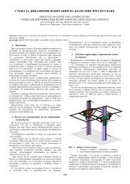
automatic inspection of single-system-mélange color fabric density ...
automatic inspection of single-system-mélange color fabric density ...
automatic inspection of single-system-mélange color fabric density ...

Create successful ePaper yourself
Turn your PDF publications into a flip-book with our unique Google optimized e-Paper software.
AUTOMATIC INSPECTION OF SINGLE-SYSTEM-MÉLANGE COLOR FABRIC<br />
DENSITY BASED ON FCM ALGORITHM<br />
Gao Weidong 1,2 , Wang Shanyuan 1 , Pan Ruru 2 , Liu Jihong 2 , Wang Xuefang 2 , Lei Hui 2<br />
1 College <strong>of</strong> Textile, Donghua University, Shanghai, China<br />
2 Key Laboratory <strong>of</strong> Eco-Textiles, School <strong>of</strong> Textile and Clothing, Jiangnan University, Wuxi, Jiangsu, China<br />
Abstract: According to the <strong>color</strong> yarns in the <strong>fabric</strong>, the <strong>fabric</strong>s can be divided into three categories: solid <strong>color</strong> <strong>fabric</strong>s, <strong>single</strong>-<strong>system</strong><strong>mélange</strong><br />
<strong>color</strong> <strong>fabric</strong>s and double-<strong>system</strong>-<strong>mélange</strong> <strong>color</strong> <strong>fabric</strong>s. In Part I <strong>of</strong> this study, we have used Hough transform to detect the <strong>density</strong><br />
<strong>of</strong> solid <strong>color</strong> <strong>fabric</strong>s successfully. Based on the research, we will discuss the method for detecting the <strong>density</strong> <strong>of</strong> <strong>single</strong>-<strong>system</strong>-<strong>mélange</strong> <strong>color</strong><br />
<strong>fabric</strong>s in this paper. By analyzing the pattern and <strong>color</strong> characters <strong>of</strong> <strong>single</strong>-<strong>system</strong>-<strong>mélange</strong> <strong>color</strong> <strong>fabric</strong>s, FCM algorithm is proposed to<br />
classify the <strong>color</strong>s in the <strong>fabric</strong> image based on Lab <strong>color</strong> space first. With the <strong>color</strong> segmentation results, the <strong>fabric</strong> can be divided into<br />
different blocks. The yarns can be located in different blocks with different means, and then the number <strong>of</strong> yarns can be counted. The <strong>fabric</strong><br />
<strong>density</strong> can be obtained by counting the yarns in a unit length finally. The experiment proved that the algorithm proposed in this study can<br />
inspect the <strong>density</strong> <strong>of</strong> <strong>single</strong>-<strong>system</strong>-<strong>mélange</strong> <strong>color</strong> <strong>fabric</strong> successfully.<br />
Keywords: FABRIC DENSITY, SINGLE-SYSTEM-MÉLANGE COLOR FABRIC, FCM ALGORITHM, LAB COLOR<br />
SPACE, COLOR CLASSIFICATION.<br />
1. Introduction<br />
In previous study, we proposed to use Hough transform to<br />
detect the skew angles <strong>of</strong> warp and weft yarns in the <strong>fabric</strong>. And<br />
then gray-projection method was selected to locate the yarns in the<br />
<strong>fabric</strong> image. The experiment showed that the <strong>density</strong> <strong>of</strong> solid <strong>color</strong><br />
<strong>fabric</strong>s can be inspected <strong>automatic</strong>ally [1] . However, the method can<br />
be only applied for solid <strong>color</strong> <strong>fabric</strong>s, and it can’t inspect the<br />
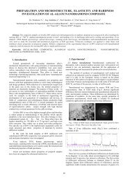
<strong>density</strong> <strong>of</strong> the <strong>fabric</strong>s with more than two <strong>color</strong>s. Figure 1 shows<br />
one sample <strong>of</strong> the <strong>fabric</strong> with four <strong>color</strong>s. It’s obviously that gray-<br />
projection can not be applied to the regions including more that two<br />
<strong>color</strong> yarns. The methods for measuring the <strong>fabric</strong> <strong>density</strong><br />
mentioned in literature [2-7] can not inspect the <strong>density</strong> <strong>of</strong> <strong>fabric</strong> with<br />
more than two <strong>color</strong>s.<br />
Fig. 1 Fabric image with several <strong>color</strong> yarns.<br />
In Part I, we divided the <strong>color</strong> <strong>fabric</strong>s into two categories: one<br />
group is <strong>single</strong>-<strong>system</strong>-<strong>mélange</strong> <strong>color</strong> <strong>fabric</strong> as shown in Figure 1.<br />
There are more that two <strong>color</strong>s in the <strong>fabric</strong>. But one group <strong>of</strong> yarns,<br />
weft or warps, are constituted by one kind <strong>of</strong> <strong>color</strong> yarns. For<br />
example, the warps in the <strong>fabric</strong> shown in Figure 1 are all white<br />
yarns, while the wefts are composed by four kinds <strong>of</strong> different <strong>color</strong><br />
yarns.<br />
Fig. 2 Double-<strong>system</strong>-<strong>mélange</strong> <strong>color</strong> <strong>fabric</strong> image.<br />
Another group is double-<strong>system</strong>-<strong>mélange</strong> <strong>color</strong> <strong>fabric</strong> as<br />
shown in Figure 2. It is also composed by more that two kinds <strong>of</strong><br />
<strong>color</strong> yarns. But both the wefts and warps are made up by more than<br />
two kinds <strong>of</strong> <strong>color</strong> yarns. In this study, we just discuss the method<br />
for inspecting the <strong>density</strong> <strong>of</strong> the first category. The second category,<br />
51<br />
<strong>of</strong> course, the most complicated <strong>fabric</strong>s, will be discussed in future<br />
study.<br />
FCM algorithm has been used to analyze the <strong>color</strong> segmentation<br />
for printed <strong>fabric</strong>s in RGB <strong>color</strong> model [8] . By the unsupervised<br />
clustering method, the <strong>color</strong>s were classified successfully. We have<br />
tried to use an improved FCM algorithm to segment the <strong>color</strong>s in<br />
yarn-dyed <strong>fabric</strong>s in HSL <strong>color</strong> space [9] . But in further study, we<br />
found that RGB and HSL <strong>color</strong> models have their own fault for<br />
<strong>color</strong> classification. And the experiment shows that in these two<br />
<strong>color</strong> spaces, some <strong>color</strong> <strong>fabric</strong> images can not be classified with<br />
satisfied results. Take the <strong>fabric</strong> shown in Figure 1 as an example,<br />
the <strong>color</strong>s are classified with FCM algorithm in HSL and RGB<br />
<strong>color</strong> space, and the classification results were shown in Figure 3.<br />
Compared with the original image, it can be seen that the blue<br />
and gray yarns have been segmented, but the green and white yarns<br />
are not segmented successfully in the two <strong>color</strong> spaces. The borders<br />
<strong>of</strong> the green and white yarns in the classification results are very<br />
vague, and it is hard to locate the yarns with <strong>color</strong> classification<br />
results. The expectation results have not been obtained. In order to<br />
find the reasons, we checked the <strong>fabric</strong> image in Photoshop<br />
s<strong>of</strong>tware, and found that the white and green yarns in Figure 1 have<br />
similar hue and intensity values. Therefore, it is hard to separate<br />
them from each other in RGB and HSL <strong>color</strong> spaces. In order to<br />
solve this problem, CIE-Lab <strong>color</strong> space is proposed to classify the<br />
<strong>color</strong>s in the <strong>fabric</strong> image with FCM algorithm. With the <strong>color</strong><br />
segmentation results, the <strong>fabric</strong> image can be segmented into<br />
different blocks, and the yarns are located in different blocks with<br />
different means. The <strong>fabric</strong> <strong>density</strong> can be obtained by counting the<br />
yarns in a unit length with an <strong>automatic</strong> method at last.<br />
(a) RGB <strong>color</strong> model (b)HSL <strong>color</strong> model<br />
Fig. 3 Color classification results <strong>of</strong> <strong>fabric</strong> image.<br />
2. CIE-Lab Color Model<br />
Compared with RGB and HSL <strong>color</strong> models, Lab <strong>color</strong> model is<br />
designed to approximate human vision. Its model is shown in<br />
Figure 4. Lab model aspires to perceptual uniformity, and its L<br />
component closely matches human perception <strong>of</strong> lightness. It can
thus be used to make accurate <strong>color</strong> balance correction by<br />
modifying output curves with a and b components, or adjusting the<br />
lightness contrast using L component. But in RGB <strong>color</strong> model or<br />
HSL <strong>color</strong> model, it is hard to realize these.<br />
Fig. 4 Lab Color Space.<br />
2.1 Conversation From RGB to Lab<br />
In the computer, the image is expressed or saved in RGB <strong>color</strong><br />
model. To use Lab <strong>color</strong> model, the first step is to convert the image<br />
from RGB to Lab <strong>color</strong> space in the experiment. To complete the<br />
conversion, the <strong>fabric</strong> image should first be changed to XYZ <strong>color</strong><br />
model. The conversion method is given as follows:<br />
(1)r=R/255<br />
(2)<br />
⎛r+ 0.055 ⎞<br />
if(<br />
r > 0.04045) r = ⎜ ⎟<br />
⎝ 1.055 ⎠<br />
r<br />
else r =<br />
12.92<br />
To obtain g, b, the G, B components are processed in the same<br />
way.<br />
⎡X⎤ ⎡0.4124 0.3576 0.1805⎤<br />
⎡r⎤ (3) ⎢Y ⎥ = ⎢0.2106 0.7125 0.0722⎥⋅⎢g⎥<br />
⎢ ⎥ ⎢ ⎥ ⎢ ⎥<br />
⎢⎣Z⎥⎦ ⎢⎣0.0193 0.1192 0.9505⎥⎦<br />
⎢⎣b⎥⎦ After then, the image can be converted to Lab from RGB <strong>color</strong><br />
space with the help <strong>of</strong> XYZ <strong>color</strong> model in follow steps:<br />
(1) f( X 0.008856) x X<br />
else<br />
16<br />
x = 7.787 × X +<br />
116<br />
1<br />
3<br />
i > = ,<br />
(2)Y, Z components are processed as X component in step 1, and we<br />
can get y, z.<br />
⎧ L = 116 × y−16<br />
(3) ⎪<br />
⎨a<br />
= 500 × ( x− y)<br />
⎪<br />
⎩b<br />
= 200 × ( y− z)<br />
After the conversion, L, a, b are all belong to [-128, 128],<br />
thus cluster method can be used to classify the <strong>color</strong>s in the <strong>single</strong><strong>system</strong>-<strong>mélange</strong><br />
<strong>color</strong> <strong>fabric</strong> image with Lab <strong>color</strong> space. The Lab<br />
image <strong>of</strong> the sample <strong>fabric</strong> is shown in Figure 5. The green and<br />
white yarns which are difficult to classify in RGB and HSL <strong>color</strong><br />
space, are now easily to distinguish in Lab image. And it provides<br />
the foundation <strong>of</strong> segmentation for the <strong>color</strong> yarns in <strong>single</strong>-<strong>system</strong><strong>mélange</strong><br />
<strong>color</strong> <strong>fabric</strong>s.<br />
2.2 Conversion from Lab to RGB<br />
To show the segmentation results, the <strong>fabric</strong> image should be<br />
changed back from Lab to RGB <strong>color</strong> space. The method is similar<br />
as mentioned above. It is the inverse process. The <strong>fabric</strong> image<br />
2.4<br />
,<br />
52<br />
should first be changed to XYZ <strong>color</strong> model, and then converted<br />
back to RGB <strong>color</strong> model to shown on the screen.<br />
Fig. 5 Lab Image <strong>of</strong> Figure 1.<br />
3. Fuzzy C-Means Clustering Method<br />
In the <strong>color</strong> segmentation and pattern recognition, clustering is<br />
one <strong>of</strong> the most important processes. Among the clustering<br />
methods, Fuzzy C-Means clustering method (FCM) is most famous.<br />
FCM algorithm [10] is an unsupervised clustering method. The<br />
clustering method attempts to minimize the objective function by<br />
organizing the data into different clusters. The objective function is<br />
as follow:<br />
c n<br />
∑∑<br />
m<br />
JUV ( , ) = uij x −v<br />
i= 1 j=<br />
1<br />
j i<br />
where n is the number <strong>of</strong> data; c is the cluster number; U is the<br />
memberships degree matrix; V is the cluster centers matrix; u ij<br />
expresses the membership degree <strong>of</strong> the data point x j belonging to<br />
the ith fuzzy group. u ij satisfies these two conditions:<br />
u ∈ [0,1], i = 1,2,..., c and<br />
ij<br />
c<br />
∑<br />
i=<br />
1<br />
u = 1, j = 1,2,..., n.<br />
m ∈ (1, +∞ ) is a weighting exponent that influences the<br />
fuzziness <strong>of</strong> the clusters. It controls the sharing degree between<br />
different cluster groups.<br />
FCM algorithm <strong>of</strong>ten starts with an initial guess for the cluster<br />
centers [11] which is intended to mark the mean location <strong>of</strong> each<br />
cluster. The initial guess for these cluster centers will most likely be<br />
incorrect. So in the experiment we choose to initial the membership<br />
matrix. The FCM algorithm is implemented as follows [12] :<br />
(1)Choose the cluster number c, the weighting exponent m and the<br />
terminative precision ε .<br />
(2)Initialize the membership degree matrix U (0) and set the iteration<br />
counter t=1.<br />
(3)Update the cluster center matrix using membership degree<br />
matrix:<br />
n<br />
i = ∑<br />
m<br />
ij<br />
n<br />
m<br />
j / ∑ ij , = 1,2,...,<br />
j= 1 j=<br />
1<br />
v u x u i c<br />
(4)Update the membership degree matrix U, and set t=t+1..<br />
u<br />
ij<br />
2<br />
−1<br />
⎡ ⎤<br />
c m−1<br />
⎢ ⎛ d ⎞ ij ⎥<br />
∑<br />
=<br />
⎢ ⎜<br />
⎟<br />
k = 1 d ⎟ ⎥<br />
⎝ kj ⎢ ⎠<br />
⎣ ⎥⎦<br />
If d = 0 , u = 1,<br />
and u = 0( i ≠ k)<br />
.<br />
kj<br />
kj<br />
ij<br />
Here<br />
d x v<br />
2<br />
ij = || i − j || .<br />
ij<br />
2
( t+ 1) ( t)<br />
(5)If U −U ≤ ε , stop the iteration, otherwise go to step 3.<br />
4. Experiments<br />
4.1 Fabric Image Acquisition<br />
A Microtek flat scanner was used to digitize the <strong>single</strong>-<strong>system</strong><strong>mélange</strong><br />
<strong>color</strong> <strong>fabric</strong> image with a resolution <strong>of</strong> 1200 DPI. Just as<br />
the solid <strong>color</strong> <strong>fabric</strong>, in order to reduce the <strong>color</strong> differentiation on<br />
the <strong>fabric</strong>’s appearance, the capture region was selected far from the<br />
edge <strong>of</strong> the <strong>fabric</strong>, and the surface <strong>of</strong> <strong>fabric</strong> should be clarity in the<br />
experiment.<br />
4.2 Detect The Skew Angle <strong>of</strong> Yarns<br />
According to the method discussed in previous study, Hough<br />
transform is used to detect the skew angles <strong>of</strong> warps and wefts, and<br />
they are marked as θ warp and θ weft , where θ warp represents the<br />
skew angle <strong>of</strong> warps while θ weft is the skew angle <strong>of</strong> wefts.<br />
4.3 Color Classification in Lab Color Space<br />
As discussed above, the <strong>fabric</strong> image is converted from RGB to<br />
Lab <strong>color</strong> model, and then FCM algorithm is used to classify the<br />
<strong>color</strong>s in <strong>fabric</strong> image. Take the <strong>fabric</strong> image shown in Figure 1 as<br />
an example, set the cluster number c =4, weighting exponent m =2,<br />
the terminative precision ε =0.001. The <strong>color</strong> classification result is<br />
shown in Figure 6.<br />
Fig. 6 Color classification result in Lab <strong>color</strong> space.<br />
From Figure 6, it can be found that Lab <strong>color</strong> space has its<br />
inherent advantages in <strong>color</strong> classification. Compared with the<br />
results in RGB and HSL <strong>color</strong> spaces as shown in Figure 3, the<br />
<strong>color</strong> segmentation result in Lab <strong>color</strong> space is more superior.<br />
However, there still are some gray pixels in the white yarn block in<br />
the result. It may be caused by undulating weave structure or other<br />
reasons. In order to eliminate these pixels, the image was converted<br />
from RGB model to gray model. Closed operation was used to<br />
process the image in gray model. A 3× 3 filter was selected in the<br />
experiment. The processing result was shown in Figure 7. From the<br />
figure, it can be seen that the noise has been removed successfully.<br />
Fig. 7 Closed operation processing result.<br />
4.4 Divide The Fabric Image into Different Blocks<br />
With the <strong>color</strong> classification results, the <strong>fabric</strong> can be divided<br />
into several blocks which include one kind <strong>of</strong> weft yarns. As one<br />
group <strong>of</strong> the yarns is composed <strong>of</strong> one <strong>color</strong>, it is easy to locate the<br />
yarns in different blocks. The warps in the <strong>fabric</strong> shown in Figure 1<br />
are all white yarns. With the skew angles which have been detected,<br />
53<br />
the <strong>fabric</strong> image can be divided into eleven blocks as shown in<br />
Figure 8.<br />
Fig. 8 Eleven blocks <strong>of</strong> the <strong>fabric</strong> image.<br />
From the figure, it is observed that the blocks can be divided<br />
into two categories. One group is A, E, K, the wefts and the warps<br />
are the same <strong>color</strong> in these blocks. Another group is B, D, F, G, H,<br />
I, J, the warps and wefts have different <strong>color</strong>s. The yarns can be<br />
located in different blocks with different means, and then <strong>fabric</strong><br />
<strong>density</strong> can be inspected.<br />
5. Results and Discussion<br />
5.1 Weft Segmentation<br />
The regions where the wefts and warps have the same <strong>color</strong> can<br />
be seen as solid <strong>color</strong> <strong>fabric</strong>. This kind <strong>of</strong> <strong>fabric</strong> has been discussed<br />
in Part I. With the gray-projection method, the yarns can be<br />
segmented successfully.<br />
The gray-projection can not be applied for the blocks where<br />
wefts and warps have different <strong>color</strong>s, such as Block I. In order to<br />
locate the yarns in these blocks, correlation coefficient method is<br />
introduced into the <strong>inspection</strong> process. Suppose X, Y are two<br />
independent vectors, the correlation coefficient r <strong>of</strong> X, Y can be<br />
defined as:<br />
( X − X) ⋅( Y −Y)<br />
r =<br />
,<br />
D( X) ⋅ DY ( )<br />
where X , DX ( ) is the mean value and variance value <strong>of</strong> vector<br />
X , and Y , DY ( ) is the mean value and variance value <strong>of</strong> vector<br />
Y .<br />
r ∈− [ 1,1] is the correlation coefficient <strong>of</strong> X, Y , it represents<br />
correlation degree between the two vectors .<br />
With the skew angle which has been detected, the coordinate <strong>of</strong><br />
the pixels in the <strong>fabric</strong> image can be transformed according to the<br />
method that has been discussed in Part I <strong>of</strong> the study. Suppose ij P<br />
is the gray level <strong>of</strong> the pixel ( i, j ) , set X = ( P , P , P , ⋅⋅⋅ , P ) ,<br />
i0 i1 i 2 iw<br />
Y = ( P , P , P , ⋅⋅⋅ , P ), j = i+<br />
1.<br />
X, Y represent the adjacent<br />
j 0 j1 j 2 jw<br />
rows <strong>of</strong> pixels in the <strong>fabric</strong> image. The correlation coefficient <strong>of</strong><br />
X, Y then would be calculated. Take the Block I as an example,<br />
the correlation coefficients are shown in Figure 9.<br />
It is obvious that if the two rows are in the same yarn, r is<br />
closed to 1. If the two rows lied in the interstices between two<br />
yarns, the correlation coefficient r must be the minimum value<br />
among the adjacent points in Figure 9. Compare with Block I, the<br />
valley points in Figure 9 are corresponding to the interstices in the
<strong>fabric</strong> image. The yarns can be located by finding the local<br />
minimums in Figure 9.<br />
Fig. 9 Correlation coefficients <strong>of</strong> the adjacent rows.<br />
However, there are some error local minimums in the curve. In<br />
order to eliminate these points, a 1× 5 filter [0, 0,1, 0, 0] was used<br />
in the experiment. If the point is the minimum among the adjacent<br />
five points, it was considered as the true minimum which represents<br />
the interstice between yarns. Blocks B, D, F, G, H, J are processed<br />
with the same method then. Combine with segmentation results <strong>of</strong><br />
blocks A, E, K, the wefts in the <strong>fabric</strong> image are all segmented<br />
successfully as shown in Figure 10(a).<br />
5.2 Warp Segmentation<br />
The segmentation <strong>of</strong> warps can also be divided into two cases.<br />
Just as the weft segmentation, the block as A, E, K is considered as<br />
solid <strong>color</strong> <strong>fabric</strong>. It can be extended into the entire image. The<br />
block which composed by different <strong>color</strong> yarns can be inspected<br />
with the correlation coefficient method. The warps <strong>of</strong> the <strong>fabric</strong><br />
shown in Figure 1 are segmented successfully in Figure 10(b).<br />
(a) Weft segmentation result (b)Warp segmentation result<br />
Fig. 10 Yarn segmentation results.<br />
5.3 Inspect Fabric Density<br />
As the wefts and warps are all located in the <strong>fabric</strong> image, the<br />
<strong>fabric</strong> <strong>density</strong> can be obtained by counting the yarns in a unit<br />
length. The <strong>fabric</strong> <strong>density</strong> is also measured with a textile analysis<br />
magnifying glass manually. The results measured by these two<br />
methods are compared in Table 1. From the table, it can be seen the<br />
error is just 0.1 thread. The result measured by image analysis is<br />
very close to manual measuring result. This fact proves that the<br />
method proposed in this study can be used to measure the <strong>fabric</strong><br />
<strong>density</strong> instead <strong>of</strong> the traditional means.<br />
Table 1: The measurement <strong>of</strong> <strong>fabric</strong> <strong>density</strong><br />
Warp <strong>density</strong>[thd/inch] Weft <strong>density</strong>[thd/inch] Error[%]<br />
Automatic Manual Automatic Manual Warp Weft<br />
82.6 82.5 128.6 128.5 0.12 0.1<br />
6. Conclusions<br />
The method for inspecting the <strong>single</strong>-<strong>system</strong>-<strong>mélange</strong> <strong>color</strong><br />
<strong>fabric</strong> <strong>density</strong> was discussed in this study. The <strong>fabric</strong> sample shown<br />
in this study has same <strong>color</strong> warps and different <strong>color</strong> wefts. The<br />
<strong>density</strong> <strong>of</strong> the <strong>fabric</strong> with same <strong>color</strong> wefts and different <strong>color</strong><br />
warps can also be detected with this method by adjusting the<br />
algorithm.<br />
In this study, FCM algorithm is proposed to classify the <strong>color</strong>s<br />
for the <strong>fabric</strong> in Lab <strong>color</strong> space. By the <strong>color</strong> classification results,<br />
the <strong>fabric</strong> image can be divided into different blocks with same<br />
54<br />
<strong>color</strong> or different <strong>color</strong>s. And the gray-projection and correlation<br />
coefficient methods are used to locate the yarns in different blocks.<br />
The wefts and warps were located and the <strong>density</strong> was obtained by<br />
counting the yarns in a unit length finally. The experiment result<br />
proved the algorithm proposed can inspect the <strong>density</strong> <strong>of</strong> <strong>single</strong><strong>system</strong>-<strong>mélange</strong><br />
<strong>color</strong> <strong>fabric</strong> successfully.<br />
Till then, we have completed the measurement <strong>of</strong> the <strong>density</strong> for<br />
solid <strong>color</strong> <strong>fabric</strong>s and <strong>single</strong>-<strong>system</strong>-<strong>mélange</strong> <strong>color</strong> <strong>fabric</strong>s.<br />
According to the classification <strong>of</strong> <strong>fabric</strong>s mentioned in Part I, we<br />
still have to inspect the <strong>density</strong> <strong>of</strong> double-<strong>system</strong>-<strong>mélange</strong> <strong>color</strong><br />
<strong>fabric</strong>s. It is the most complicated <strong>fabric</strong> which discussed in this<br />
study, and the method will be described with detail in Part III <strong>of</strong> this<br />
study.<br />
Acknowledgement<br />
The authors are grateful for the financial supported by the<br />
Fundamental Research Funds for the Central Universities<br />
(No.JUSRP21105) and the National Natural Science Foundation <strong>of</strong><br />
China (No.61040046).<br />
References<br />
[1]Pan R, Gao W, Liu J, et al. Automatic <strong>inspection</strong> <strong>of</strong> woven <strong>fabric</strong><br />
<strong>density</strong> <strong>of</strong> solid colour <strong>fabric</strong> <strong>density</strong> by the Hough transform.<br />
Fibers & Textiles in Eastern Europe, 2010, 18(4):46-51.<br />
[2]Xu B. Identifying <strong>fabric</strong> structures with fast Fourier transform<br />
techniques. Textile Research Journal, 1996(66):496 - 506.<br />
[3]Hosseini Ravandi S A, Toriumi K. Fourier transform analysis <strong>of</strong><br />
plain weave <strong>fabric</strong> appearance. Textile Research Journal,<br />
1995(65): 676 - 683.<br />
[4]Lin J. Applying a co-occurrence matrix to <strong>automatic</strong> <strong>inspection</strong><br />
<strong>of</strong> weaving <strong>density</strong> for woven <strong>fabric</strong>s. Textile Research<br />
Journal, 2002(72):486-490<br />
[5]Kang T J, Kim C H, Oh K W. Automatic recognition <strong>of</strong> <strong>fabric</strong><br />
weave patterns by digital image analysis. Textile Research<br />
Journal, 1999(69):77-83<br />
[6]Huang C C, Liu S C, Yu W H. Woven <strong>fabric</strong> analysis by image<br />
processing. Part I: Identification <strong>of</strong> weave patterns. Textile<br />
Research Journal, 2000(70):481-485.<br />
[7] Jeon B S, Bae J H, Suh M W. Automatic recognition <strong>of</strong> woven<br />
<strong>fabric</strong> patterns by an artificial neural network. Textile Research<br />
Journal, 2003(73):645-650.<br />
[8]Kuo C-F J, Shih C-Y, Kao C-Y, et al. Color and pattern Analysis<br />
<strong>of</strong> Printed Fabric by an Unsupervised Clus- tering Method.<br />
Textile Research Journal, 2005(75):9-12.<br />
[9]Pan R, Gao W, Liu J. Color clustering analysis <strong>of</strong> yarn-dyed<br />
<strong>fabric</strong> in HSL <strong>color</strong> space. IEEE, World Congress on S<strong>of</strong>tware<br />
Engineering, 2009, 273-278<br />
[10]Wong C C, Chen C C, Su M C. A novel algorithm for data<br />
clustering. Pattern Recognition, 2001(34):425-442<br />
[11]Bezdek J C. Pattern recognition with fuzzy objective function<br />
algorithm, Plenum Press, NY, 1981.<br />
[12]Kuo C-F J, Shih C-Y, Lee J-Y. Automatic recognition <strong>of</strong> <strong>fabric</strong><br />
weave patterns by a fuzzy C-Means clustering method. Textile<br />
Research Journal, 2004(74):107-111.