Transition between extended and localized states in a one ...

DIENER, GEORGAKIS, ZHONG, RAIZEN, AND NIU PHYSICAL REVIEW A 64 033416
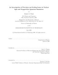
FIG. 5. In the top panel we have plotted the energy versus
momentum for the energy eigenstates of a particle moving in the
periodic potential 3.3. The points are gray-scale coded, with the
gray scale describing the probability of measuring a value of the
momentum for an eigenstate of the given energy. In the bottom
panel, we have plotted the free-particle parabola thicker line together
with the same parabola shifted by integer multiples of 1/2.
probability of a particular Bragg scattering, with the gray
scale fading as a higher number of scatterings are needed.
Notice that if the points were not gray-scale coded in the
figure, we would simply obtain the band structure of the
system in the repeated-zone scheme 1.
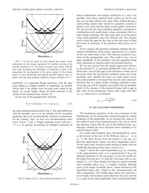
In the case of the quasiperiodic potential
Vx0.1cosx1cosx, 3.5
the same plotting method renders Fig. 6. The main difference
with the periodic case is in the location of the secondary
parabolas; these are not periodically centered in momentum.
On the contrary, since we have two incommensurate basis
wave vectors, 1 and , Bragg scattering occurs with p
1,. In general, accounting for multiple scattering, all
FIG. 6. Same as Fig. 5, but using the potential 3.5.
033416-4
linear combinations with integer coefficients of 1 and are
possible. Since these numbers form a dense set on the real
line, p can take almost any value. Thus, without the grayscale-coding
scheme there would be a parabola centered at
almost every point and the figure would appear featureless.
We can see that the most important parabolas correspond to
combinations with small integer values, associated with loworder
Bragg scattering. The main gaps open up at the points
where these parabolas meet the primary one. The integers
used to label the gaps are the same as the ones used to label
the center of symmetry of the parabola which gives rise to
them.
At low energies the potential completely reshapes the momentum
distribution of the energy eigenvectors; as a matter
of fact the states deep in the wells become localized in position
in the quasiperiodic case. This result is true even at
large amplitudes of the potential, with the parabolas being
more prominent at energies above the potential barriers.
We can now picture how the energy eigenvectors behave
as the potential V0 is increased adiabatically from zero to a
fixed value. Each of the gaps in the spectrum is borne out of
the point where the free-particle parabola meets one of the
secondary ones. Initially the states are nearly plane waves,
but as the potential is increased they become more and more
distorted, due to a large number of Bragg scattering events.
Every gap can still be uniquely associated with the parabola
which in the absence of the potential brings forth a gap at
that value of the momentum. Notice that a gap with label
(n 1 ,n 2) opens up at a momentum
pn1 ,n
2 n1n 2
. 3.6
2
IV. LOCALIZATION PROPERTIES
The localization properties of the wave functions of the
Hamiltonian can be numerically studied through the scaling
properties of the bandwidths. As we increase the value of n,
the width of each of the bands decreases. The way in which
this decrease scales with the size of the Brillouin zone (q n)
indicates whether the wave functions show extended or localized
behavior 20.
For a band with extended states, the bandwidth B n scales
as the inverse of the size of the Brillouin zone q n 1 ,oras
q n 2 if the band derives from the bottom or the top of a
previous approximant where van Hove singularities arise.
On the other hand, localized states belong to bands with the
bandwidth decreasing faster than a power of q n .
Figure 7 shows the scaled bandwidth B nq n as a function
of the approximation order n (n is proportional to ln q n) for
different situations. In the top panel, we plot the results for
the bands between the (1,1) and the (2,0) gaps with an amplitude
V 00.5. These display the behavior typical of bands
with extended states; B nq n is roughly constant, although
some of the bands eventually show a linear decrease in the
logarithmic-linear plot, related to the aforementioned van
Hove singularities. The middle panel shows the result for a
set of bands with localized states between the (0,2) and the
(1,1) gaps for the same amplitude. These scaled bandwidths