Ph.D. Thesis - Physics

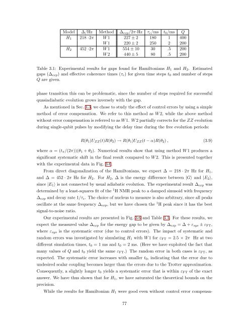
Model ∆/Hz Method ∆exp/2π·Hz τe/ms t0/ms Q
H1 218 ·2π W1 227 ± 2 180 1 400
W1 220 ± 2 250 2 200
H2 452 ·2π W1 554 ± 10 30 .5 200
W2 440 ± 5 80 .5 200
Table 3.1: Experimental results for gaps found for Hamiltonians H1 and H2. Estimated
gaps (∆exp) and effective coherence times (τe) for given time steps t0 and number of steps
Q are given.
phase transition this can be problematic, since the number of steps required for successful
quasiadiabatic evolution grows inversely with the gap.
As mentioned in Sec. 3.3, we chose to study the effect of control errors by using a simple
method of error compensation. We refer to this method as W2, while the above method
without error compensation is referred to as W1. W2 partially corrects for the ZZ evolution
during single-qubit pulses by modifying the delay time during the free evolution periods:
R(θ1)UZZ(t)R(θ2) → R(θ1)UZZ(t − α)R(θ2) , (3.9)
where α = (tπ/(2π))(θ1 + θ2). Numerical results show that using method W1 produces a
significant systematic shift in the final result compared to W2. This is presented together
with the experimental data in Fig. 3-6.
From direct diagonalization of the Hamiltonians, we expect ∆ = 218 · 2π Hz for H1,
and ∆ = 452 · 2π Hz for H2. For H2, ∆ is the energy difference between |G〉 and |E2〉,
since |E1〉 is not connected by usual adiabatic evolution. The experimental result ∆exp was
determined by a least-squares fit of the 1 H NMR peak to a damped sinusoid with frequency
∆exp and decay rate 1/τe. The choice of nucleus to measure is also arbitrary, since all peaks
oscillate at the same frequency ∆exp, but we have chosen the 1 H peak since it has the best
signal-to-noise ratio.
Our experimental results are presented in Fig. 3-6 and Table 3.1. For these results, we
expect the measured value ∆exp for the energy gap to be given by ∆exp = ∆ + εsys ± εFT,
where εsys is the systematic error (due to control errors). The impact of systematic and
random errors was investigated by simulating H1 with W1 for εFT = 2.5 × 2π Hz at two
different simulation times, t0 = 1 ms and t0 = 2 ms. (Here we have exploited the fact that
many values of Q and t0 yield the same εFT.) The random error in both cases is εFT, as
expected. The systematic error increases with smaller t0, indicating that the error due to
undesired scalar coupling becomes larger than the errors due to the Trotter approximation.
Consequently, a slightly longer t0 yields a systematic error that is within εFT of the exact
answer. We have thus shown that for H1, we have saturated the theoretical bounds on the
precision.
While the results for Hamiltonian H1 were good even without control error compensa-
77