Antti Lehtinen Doppler Positioning with GPS - Matematiikan laitos

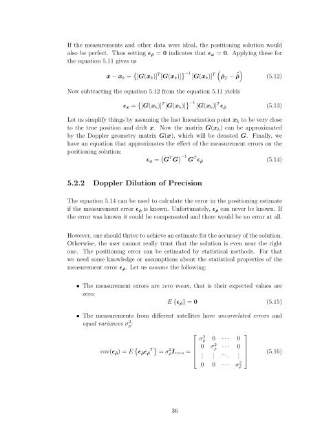
If the measurements and other data were ideal, the positioningsolution would
also be perfect. Thus setting ɛ ˙ρ = 0 indicates that ɛx = 0. Applyingthese for
the equation 5.11 gives us
x − xk = [G(xk)] T [G(xk)] −1 [G(xk)] T
˙ρ T − ˆ˙ρ (5.12)
Now subtractingthe equation 5.12 from the equation 5.11 yields
ɛx = [G(xk)] T [G(xk)] −1 [G(xk)] T ɛ ˙ρ
(5.13)
Let us simplify things by assuming the last linearization point xk to be very close
to the true position and drift x. Now the matrix G(xk) can be approximated
by the Doppler geometry matrix G(x), which will be denoted G. Finally, we
have an equation that approximates the effect of the measurement errors on the
positioningsolution:
ɛx = G T G −1 T
G ɛ ˙ρ
(5.14)
5.2.2 Doppler Dilution of Precision
The equation 5.14 can be used to calculate the error in the positioningestimate
if the measurement error ɛ ˙ρ is known. Unfortunately, ɛ ˙ρ can never be known. If
the error was known it could be compensated and there would be no error at all.
However, one should thrive to achieve an estimate for the accuracy of the solution.
Otherwise, the user cannot really trust that the solution is even near the right
one. The positioningerror can be estimated by statistical methods. For that
we need some knowledge or assumptions about the statistical properties of the
measurement error ɛ ˙ρ. Letusassume the following:
• The measurement errors are zero mean, that is their expected values are
zero:
E {ɛ ˙ρ} = 0 (5.15)
• The measurements from different satellites have uncorrelated errors and
equal variances σ 2 ˙ρ:
cov(ɛ ˙ρ) =E ɛ ˙ρɛ ˙ρ T = σ 2 ⎢
˙ρIn×n = ⎢
⎣
36
⎡
σ2 ˙ρ 0 ··· 0
0 σ2 ˙ρ ··· 0
.
.
...
0 0 ··· σ 2 ˙ρ
.
⎤
⎥
⎦
(5.16)