Antti Lehtinen Doppler Positioning with GPS - Matematiikan laitos
Antti Lehtinen Doppler Positioning with GPS - Matematiikan laitos
Antti Lehtinen Doppler Positioning with GPS - Matematiikan laitos

Create successful ePaper yourself
Turn your PDF publications into a flip-book with our unique Google optimized e-Paper software.
TAMPERE UNIVERSITY OF TECHNOLOGY<br />
Department of Electrical Engineering<br />
<strong>Antti</strong> <strong>Lehtinen</strong><br />
<strong>Doppler</strong> <strong>Positioning</strong> <strong>with</strong> <strong>GPS</strong><br />
Master of Science Thesis<br />
Subject approved by the Department Council on 17.10.2001<br />
Examiners: Prof. Keijo Ruohonen (TUT)<br />
M.Sc. Paula Syrjärinne (Nokia Mobile Phones)
Preface<br />
This Master of Science thesis is the result of my research on <strong>Doppler</strong> positioning<strong>with</strong><br />
the <strong>GPS</strong>. The thesis has been written at the Tampere University of<br />
Technology between the autumn of 2001 and February of 2002.<br />
I began my work on the <strong>GPS</strong> field at the Institute of Mathematics in November<br />
2000. My very first task was to do a literature survey and find out if <strong>Doppler</strong><br />
measurements can be used to positioning<strong>with</strong> the <strong>GPS</strong>. It turned out that the<br />
field was unexplored, which gave me a possibility to develop new algorithms and<br />
theory.<br />
I would like to thank professor Keijo Ruohonen for his mathematical assistance<br />
and other help he has given throughout the work. In addition, I express my<br />
gratitude to Paula Syrjärinne, who has provided me <strong>with</strong> <strong>GPS</strong> related advice,<br />
measurement data and excellent remarks on the contents of the thesis. Nokia<br />
Mobile Phones deserves my thanks for fundingthe project. Moreover, many<br />
Nokia employees have given me valuable feedback at the workshops. I would<br />
also like to thank the personnel of the Institute of Mathematics, especially Niilo<br />
Sirola, who has helped me a lot by proofreadingthe thesis, givingme new ideas<br />
and sharinghis Matlab functions.<br />
Furthermore, I am indebted to all the people who have given me the joy of living<br />
that helped me to complete the thesis. Especially Marjo Matikainen deserves<br />
thanks for her support duringthe work.<br />
Tampere, 26th February 2002<br />
<strong>Antti</strong> <strong>Lehtinen</strong><br />
Iidesranta 3 A 4<br />
33100 Tampere<br />
Tel. 040-7291388<br />
i
Contents<br />
Abstract v<br />
Tiivistelmä vi<br />
Abbreviations and Acronyms viii<br />
Symbols ix<br />
1 Introduction 1<br />
2 The <strong>Doppler</strong> Effect 3<br />
2.1 PhysicalBackgroundandApplications ............... 3<br />
2.2 Historyof<strong>Doppler</strong>Navigation.................... 5<br />
3 The Global <strong>Positioning</strong> System 7<br />
3.1 History................................. 7<br />
3.2 TheBasicConcepts.......................... 8<br />
3.2.1 ReferenceCoordinateSystems................ 8<br />
3.2.2 Range<strong>Positioning</strong> ....................... 8<br />
3.2.3 <strong>GPS</strong>SignalStructure..................... 9<br />
3.2.4 Pseudorang e and Delta Rang e . . . . . . . . . . . . . . . . 10<br />
3.3 Pseudorange<strong>Positioning</strong> ....................... 11<br />
3.3.1 ProblemFormulation..................... 11<br />
3.3.2 SolutionProcedure ...................... 12<br />
ii
3.4 <strong>Positioning</strong>ErrorAnalysis ...................... 13<br />
3.5 Limitationsofthe<strong>GPS</strong>........................ 14<br />
4 <strong>Doppler</strong> <strong>Positioning</strong> <strong>with</strong> the <strong>GPS</strong> 16<br />
4.1 Needfor<strong>Doppler</strong><strong>Positioning</strong>..................... 16<br />
4.2 Comparisonbetween<strong>GPS</strong>andTransit ............... 17<br />
4.3 TheGoverningEquations ...................... 18<br />
4.3.1 The<strong>Doppler</strong>ShiftEquation ................. 18<br />
4.3.2 TheClockDriftError .................... 20<br />
4.3.3 Mathematical Problem Formulation . . . . . . . . . . . . . 21<br />
4.4 SymbolicMethods .......................... 23<br />
4.4.1 Solvingthe Receiver Position . . . . . . . . . . . . . . . . 23<br />
4.4.2 Existence and Uniqueness Considerations . . . . . . . . . . 23<br />
4.5 StandardNumericalMethods .................... 24<br />
4.5.1 ProblemFormulation..................... 24<br />
4.5.2 TheNewtonMethod ..................... 25<br />
4.5.3 TheGauss-NewtonMethod ................. 26<br />
4.5.4 CalculatingtheDerivativeMatrix.............. 27<br />
4.6 ProblemSpecificIterativeMethods ................. 30<br />
5 <strong>Positioning</strong> Performance 31<br />
5.1 MeasurementNoise.......................... 31<br />
5.1.1 IonosphericEffects ...................... 31<br />
5.1.2 Receiver Noise . . . . . . . . . . . . . . . . . . . . . . . . . 32<br />
5.1.3 UnknownUserVelocity.................... 32<br />
5.1.4 BiasedTimeEstimate .................... 34<br />
5.2 <strong>Positioning</strong>Accuracy......................... 35<br />
5.2.1 Effect of Measurement Errors on <strong>Positioning</strong>Solution . . . 35<br />
5.2.2 <strong>Doppler</strong> Dilution of Precision . . . . . . . . . . . . . . . . 36<br />
iii
5.2.3 Applications of the <strong>Doppler</strong> Dilution of Precision Concept 39<br />
5.3 Case of Normally Distributed Measurement Noise . . . . . . . . . 40<br />
6 Numerical Results 43<br />
6.1 MeasurementData .......................... 43<br />
6.2 PropertiesoftheMeasurementNoise ................ 44<br />
6.2.1 Hypothesis of the Properties of the Measurement Errors . 44<br />
6.2.2 Numerical Testingof Normality . . . . . . . . . . . . . . . 45<br />
6.2.3 Numerical Testingof Correlation . . . . . . . . . . . . . . 45<br />
6.2.4 MagnitudeofErrors ..................... 47<br />
6.2.5 Conclusions .......................... 48<br />
6.3 <strong>Positioning</strong>Performance<strong>with</strong>RealData .............. 48<br />
6.3.1 <strong>Positioning</strong>Accuracy..................... 48<br />
6.3.2 Convergence.......................... 50<br />
6.4 <strong>Positioning</strong>Performance <strong>with</strong> Simulated<br />
Data.................................. 50<br />
6.4.1 <strong>Positioning</strong>Accuracy..................... 51<br />
6.4.2 TheDistributionofDPDOPValues............. 51<br />
7 Conclusions 53<br />
iv
Abstract<br />
TAMPERE UNIVERSITY OF TECHNOLOGY<br />
Department of Electrical Engineering<br />
Institute of Mathematics<br />
<strong>Lehtinen</strong>, <strong>Antti</strong>: <strong>Doppler</strong> <strong>Positioning</strong><strong>with</strong> <strong>GPS</strong><br />
Master of Science thesis, 58 pages<br />
Examiners: Prof. Keijo Ruohonen and M.Sc. Paula Syrjärinne<br />
Funding: Nokia Mobile Phones<br />
March 2002<br />
Satellite positioningis expected to have hundreds of millions of users in the near<br />
future. There is a huge commercial potential in personal positioning. The standard<br />
positioningsystem nowadays is the Global <strong>Positioning</strong>System (<strong>GPS</strong>). The<br />
<strong>GPS</strong> is very accurate in good conditions. In indoors and urban areas, however,<br />
the standard <strong>GPS</strong> positioningusually fails. This decreases suitability of the <strong>GPS</strong><br />
for personal positioning.<br />
The objective of this thesis was to examine a new <strong>GPS</strong> positioningmethod based<br />
on <strong>Doppler</strong> measurements. <strong>Doppler</strong> positioning<strong>with</strong> the <strong>GPS</strong> has generally been<br />
overlooked because it provides worse accuracy than the standard method. However,<br />
the <strong>Doppler</strong> measurements can be obtained even in very bad conditions.<br />
Thus, when combined <strong>with</strong> cellular network assistance, the method may prove<br />
valuable.<br />
In this thesis, a new positioning algorithm is developed. The algorithm needs only<br />
the <strong>Doppler</strong> measurements from at least four <strong>GPS</strong> satellites, the <strong>GPS</strong> satellite<br />
orbital parameters and the current time. A general theory for estimating errors<br />
in <strong>GPS</strong> <strong>Doppler</strong> positioningis also developed. Numerical results are compared<br />
<strong>with</strong> the measurements and the accuracy of the algorithm is assessed.<br />
v
Tiivistelmä<br />
TAMPEREEN TEKNILLINEN KORKEAKOULU<br />
Sähkötekniikan osasto<br />
<strong>Matematiikan</strong> <strong>laitos</strong><br />
<strong>Lehtinen</strong>, <strong>Antti</strong>: <strong>Doppler</strong>-paikannus <strong>GPS</strong>:llä<br />
Diplomityö, 58 sivua<br />
Tarkastajat: Prof. Keijo Ruohonen ja DI Paula Syrjärinne<br />
Rahoitus: Nokia Mobile Phones<br />
Maaliskuu 2002<br />
Satelliittipaikannuksella uskotaan lähitulevaisuudessa olevan satoja miljoonia<br />
käyttäjiä. Henkilökohtainen paikannus tarjoaa suuria kaupallisia mahdollisuuksia.<br />
Tärkein paikannusjärjestelmä on nykyään Global <strong>Positioning</strong>System (<strong>GPS</strong>).<br />
Hyvissä olosuhteissa <strong>GPS</strong> on erittäin tarkka. Ongelmia aiheutuu kuitenkin siitä,<br />
että perinteinen <strong>GPS</strong>-paikannusmenetelmä ei usein toimi sisätiloissa tai kaupunkialueilla.<br />
Tämä luonnollisesti heikentää <strong>GPS</strong>:n soveltuvuutta henkilökohtaiseen<br />
paikannukseen.<br />
Tämän diplomityön tarkoituksena oli tutkia satelliittisignaalien kantoaalloista<br />
tehtävien <strong>Doppler</strong>-mittausten käyttömahdollisuutta <strong>GPS</strong>:ssä. <strong>Doppler</strong>-ilmiöön<br />
perustuvaa paikannusta on menestyksekkäästi käytetty esimerkiksi <strong>GPS</strong>:n edeltäjässä,<br />
Transit-järjestelmässä. <strong>GPS</strong>:n yhteydessä <strong>Doppler</strong>-mittausten käyttöä paikan<br />
selvittämiseen ei kuitenkaan ole käytetty, sillä paikannustarkkuuden on oletettu<br />
olevan huonompi kuin perinteisellä vale-etäisyyksiin perustuvalla menetelmällä.<br />
Vale-etäisyyksien selvittämiseksi <strong>GPS</strong>-vastaanottimen on kuitenkin kyettävä<br />
demoduloimaan satelliittien lähettämä navigointisanoma. Sen sijaan <strong>Doppler</strong>mittauksia<br />
pystytään useimmiten tekemään vaikka signaali olisikin niin vääristynyt<br />
ettei navigointisanomaa saada.<br />
Tässä diplomityössä esitetään uusi <strong>GPS</strong>-paikannusmenetelmä, jolla voidaan ratkaista<br />
vastaanottimen sijainti mittaamalla vähintään neljän <strong>GPS</strong>-satelliitin kantoaaltojen<br />
<strong>Doppler</strong>-siirtymät yhtäaikaisesti. Menetelmässä ei tarvita navigointisignaalia,<br />
joten paikannus voidaan suorittaa myös huonoissa signaaliolosuhteis-<br />
vi
sa. Satelliittien ratatiedot ja aikatieto pitää kuitenkin olla saatavilla. Mikäli navigointisanomaa<br />
ei saada, pitää vastaanottimen siis olla yhteydessä esimerkiksi<br />
matkapuhelintukiasemaan.<br />
Työssa kehitetään myös yleinen teoriapohja <strong>Doppler</strong>-paikannuksen virhetarkastelulle.<br />
Teoria on täysin uusi, mutta perustuu samoihin käsitteisiin, joita käytetään<br />
perinteisessä <strong>GPS</strong>-paikannuksessa. Teorian mukaan paikannusvirhettä estimoitaessa<br />
tarkastelu voidaan eriyttää kahteen toisistaan riippumattomaan osaan:<br />
mittausvirheiden arvioimiseen ja satelliittigeometrian vaikutuksen laskemiseen.<br />
Työssä esitetään myös paikannusvirheteorian käyttomahdollisuuksia esimerkiksi<br />
numeerisen laskennan keventämiseksi. Lisäksi arvioidaan <strong>Doppler</strong>–mittauksiin<br />
vaikuttavia virhetekijöitä sekä niiden suuruuksia.<br />
Diplomityön numeerisessa osassa uuden paikannusmenetelmän toimivuutta kokeillaan<br />
todellisen mittausaineiston avulla. Paikallaanolevalle vastaanottimelle<br />
jolla on tarkka aikatieto saadaan paikannusvirheen arvioksi 100–200 metriä. Virheen<br />
havaitaan kuitenkin riippuvan hyvin voimakkaasti satelliittien sijainnista<br />
sekä saatavilla olevien satelliittisignaalien määrästä. Huonoimmissa tapauksissa<br />
menetelmä osoittautuu antavan paikkaestimaatteja, jotka ovat miljoonien kilometrien<br />
päässä todellisesta vastaanottimen sijainnista. Hyvänä puolena on se,<br />
että työssä kehitetyn virhetarkasteluteorian avulla kyseiset tilanteet kyetään havaitsemaan.<br />
Teoria osoittautui toimivaksi myös numeeristen simulointien valossa.<br />
Tässä diplomityössä esitetty paikannusmenetelmä voisi toimia varmistusmenetelmänä<br />
perinteisen <strong>GPS</strong>-paikannuksen epäonnistuessa. Paikannusvirheen havaittiin<br />
kuitenkin olevan suurempi kuin perinteisellä menetelmällä. Virhe voi olla<br />
hyvinkin suuri silloin kun saatavilla on vain vähän satelliittisignaaleja. Lisäksi<br />
teoreettisesti on odotettavissa, että vastaanottimen liike aiheuttaa hyvin merkittävän<br />
paikannusestimaatin heikkenemisen.<br />
vii
Abbreviations and Acronyms<br />
C/A coarse/acquisition code<br />
cm centimetre<br />
DOD U.S. Department of Defence<br />
DDDOP <strong>Doppler</strong> drift dilution of precision<br />
DDOP <strong>Doppler</strong> dilution of precision<br />
DHDOP <strong>Doppler</strong> horizontal dilution of precision<br />
DGDOP <strong>Doppler</strong> geometrical dilution of precision<br />
D<strong>GPS</strong> differential <strong>GPS</strong><br />
DOP dilution of precision<br />
DPDOP <strong>Doppler</strong> position dilution of precision<br />
DVDOP <strong>Doppler</strong> vertical dilution of precision<br />
ECEF Earth-centred Earth-fixed coordinate system<br />
ECI Earth-centred inertial coordinate system<br />
GDOP geometrical dilution of precision<br />
<strong>GPS</strong> Global <strong>Positioning</strong>System<br />
Hz hertz<br />
m metre<br />
Matlab Matrix Laboratory, a mathematical software<br />
MHz megahertz<br />
PRN pseudorandom noise<br />
P(Y) precision code<br />
s second<br />
SA selective availability<br />
viii
Symbols<br />
× vector cross product<br />
• dot product, scalar product<br />
euclidian norm, 2-norm, length of a vector<br />
∂ partial derivative<br />
α angle between satellite velocity and satellite-to-user vector<br />
△f frequency measurement error caused by receiver clock drift<br />
△n vector n estimate correction in an iterative algorithm<br />
△t receiver time estimate bias<br />
△ti signal propagation time from the ith satellite<br />
△wu error in user velocity vector estimate<br />
△x vector x estimate correction in an iterative algorithm<br />
ɛ machine precision<br />
ɛ ˙ρ delta range vector measurement noise<br />
ɛρi measurement noise of pseudorange from the ith satellite<br />
ɛ ˙ρi measurement noise of delta range from the ith satellite<br />
ɛd clock drift equivalent error<br />
ɛfi satellite i frequency measurement error<br />
ɛru user position error<br />
ɛx positioningerror vector<br />
ν1,ν2 degrees of freedom<br />
ω transmitted frequency<br />
ω ′ received frequency<br />
θ angle between relative velocity and wave propagation direction<br />
˙ρ delta range measurement vector<br />
ˆρ expected pseudorange vector<br />
ˆ˙ρ expected delta range vector<br />
ρi pseudorange measurement from the ith satellite<br />
˙ρi delta range measurement from the ith satellite<br />
ˆρi expected pseudorange from the ith satellite<br />
˙ρ T true delta range vector<br />
ρTi true pseudorange from the ith satellite<br />
˙ρTi true delta range from the ith satellite<br />
σ standard deviation<br />
ix
σ2 variance, covariance<br />
a vector in R3 ai relative acceleration vector of the ith satellite <strong>with</strong> respect to the user<br />
A <strong>Doppler</strong> geometric dilution of precision matrix<br />
b vector in R3 c speed of light<br />
c vector in R3 cov covariance operator<br />
d receiver clock drift equivalent, derivative<br />
ˆd estimated receiver clock drift equivalent<br />
Di <strong>Doppler</strong> shift from the ith satellite<br />
E expectation value operator<br />
f real valued function<br />
f(ɛx) probability distribution function of positioningerror vector<br />
fi measured frequency from satellite i<br />
g real valued function<br />
G <strong>Doppler</strong> geometry matrix<br />
H pseudorange geometry matrix<br />
I identity matrix<br />
i, j, k, l satellite indexes<br />
L1 <strong>GPS</strong> civil frequency 1575.42 MHz<br />
L2 <strong>GPS</strong> military frequency 1227.6 MHz<br />
n number of satellites used in the calculations<br />
n user position and time vector<br />
ˆn estimated user position and time vector<br />
p(ˆx) delta range residuals function<br />
pi(ˆx) ith component of delta range residuals function<br />
R set of real numbers<br />
ri satellite i position vector<br />
ru user position vector<br />
ˆru estimated user position vector<br />
T matrix transpose<br />
tu receiver clock bias<br />
˙tu receiver clock drift<br />
v speed<br />
vprop wave propagation speed<br />
vrel transmitter relative speed <strong>with</strong> respect to the receiver<br />
vi estimated satellite i relative velocity vector <strong>with</strong> respect to the user<br />
wi satellite i velocity vector<br />
wTu true user velocity vector<br />
wu estimated user velocity vector<br />
x wave transmitter position<br />
x user position and drift vector<br />
ˆx estimated user position and drift vector<br />
initial guess for user position and drift vector<br />
x0<br />
x
xk<br />
xu<br />
ˆxu<br />
yu<br />
ˆyu<br />
zu<br />
ˆzu<br />
vector x estimate after k steps of an iterative algorithm<br />
user x coordinate<br />
estimated user x coordinate<br />
user y coordinate<br />
estimated user y coordinate<br />
user z coordinate<br />
estimated user z coordinate<br />
xi
Chapter 1<br />
Introduction<br />
Satellite positioninghas received much attention duringthe last 40 years. The<br />
beginningera of satellite positioningresearch was focused on military applications.<br />
Now the focus has changed. Because of the huge commercial potential,<br />
the objective of the current research is mainly to develop equipment for personal<br />
positioning.<br />
The Global <strong>Positioning</strong>System (<strong>GPS</strong>) is currently the only satellite positioning<br />
system suitable for personal positioning. The <strong>GPS</strong> is funded by the United States.<br />
A new system, called Galileo, is expected to be launched by the European Union<br />
in 2008. The Galileo is very similar to the <strong>GPS</strong>.<br />
The <strong>GPS</strong> has a very good accuracy in good conditions. However, problems arise<br />
in indoors and urban areas. The standard <strong>GPS</strong> receiver needs to track at least<br />
four satellites simultaneously. In addition, it needs to demodulate the navigation<br />
message from the carrier signals. The demodulation is possible only if the signal<br />
is not too noisy. When the demodulation fails, the position cannot be solved.<br />
This is a huge drawback for use of the <strong>GPS</strong> in personal positioning. Most of the<br />
users of the positioningservices live in urban areas.<br />
Duringthe last few years much effort has been put to solve the problem. Many<br />
innovative solutions have been explored. They are mainly based on the idea of<br />
the assisted <strong>GPS</strong>. This means that the <strong>GPS</strong> measurements are combined <strong>with</strong><br />
other data, which is available for example from cellular network.<br />
In this thesis an entirely new algorithm based on <strong>Doppler</strong> measurements is presented.<br />
<strong>Doppler</strong> positioninghas been earlier mentioned in the literature, but<br />
its value has been overlooked. The reason for the bad reputation of the <strong>GPS</strong><br />
<strong>Doppler</strong> positioningis the fact that its accuracy is expected to be worse than<br />
that of the standard positioningmethod. This may indeed be true, but no one<br />
1
has seemed to consider the use of <strong>Doppler</strong> positioningin weak signal conditions.<br />
The great benefit of the <strong>Doppler</strong> positioning is that the <strong>Doppler</strong> measurements<br />
can be received even when the standard positioningfails. The <strong>Doppler</strong> measurements<br />
can be used to solve the receiver position even <strong>with</strong>out demodulatingthe<br />
navigation message. This requires that the satellite orbital parameters and the<br />
current time are known from some other source. Thus, this thesis belongs to the<br />
field of assisted <strong>GPS</strong>.<br />
The discussion of the <strong>GPS</strong> <strong>Doppler</strong> positioningis started <strong>with</strong> the physical background<br />
of the <strong>Doppler</strong> effect in Chapter 2. The chapter also enlightens the applications<br />
of the <strong>Doppler</strong> effect in satellite positioningand other fields. Chapter<br />
3 introduces the Global <strong>Positioning</strong>System, its standard positioningalgorithm<br />
and its limitations. Chapter 4 begins by discussing the feasibility of <strong>GPS</strong><br />
<strong>Doppler</strong> positioning. Later in the chapter, the new <strong>Doppler</strong> positioning algorithm<br />
is presented. Chapter 5 turns the attention to the important issue of positioning<br />
accuracy. Possible error sources are discussed. In addition, a theory for estimating<strong>Doppler</strong><br />
positioningaccuracy is developed. The possible applications of<br />
the theory are also covered. Chapter 6 begins <strong>with</strong> a numerical analysis of the<br />
properties of the measurement noise. Later, the new theory is compared <strong>with</strong> the<br />
numerical results. Furthermore, positioningresults <strong>with</strong> real measurement data<br />
are illustrated. Finally, Chapter 7 ends the thesis <strong>with</strong> conclusions.<br />
2
Chapter 2<br />
The <strong>Doppler</strong> Effect<br />
In this chapter we will shortly discuss the <strong>Doppler</strong> effect as a physical phenomenon<br />
and introduce some of its applications in modern technology. In addition, the<br />
history of exploitingthe <strong>Doppler</strong> effect in satellite navigation is considered.<br />
2.1 Physical Background and Applications<br />
The <strong>Doppler</strong> effect was first noticed by the Austrian physicist C.J. <strong>Doppler</strong> (1803-<br />
1853). The phenomenon was first noticed in sound, but it applies to every kind<br />
of wave propagation. The <strong>Doppler</strong> effect is caused by a transmitter that is in<br />
relative motion <strong>with</strong> respect to a receiver. When the transmitter approaches the<br />
receiver, the transmitted signal is squeezed. This produces a rise in the frequency<br />
of the transmitted signal. As explained in [Alonso & Finn, p. 706] and [Giancoli,<br />
p. 321], the frequency experienced by the receiver can be modelled as<br />
ω ′ <br />
= 1 − vrel<br />
<br />
cos θ<br />
ω (2.1)<br />
vprop<br />
where ω ′ is the received frequency, ω is the transmitted frequency, vrel is the magnitude<br />
of relative velocity of the transmitter <strong>with</strong> respect to the receiver, vprop is<br />
the propagation speed of the wave and θ is the angle between the relative velocity<br />
and the wave propagation direction. The equation 2.1 is a valid approximation<br />
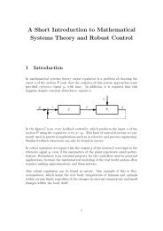
when vrel ≪ vprop. Figure 2.1 illustrates the squeezing of the signal when the<br />
transmitter located at the point x is at motion <strong>with</strong> speed v.<br />
The <strong>Doppler</strong> effect is still mostly known from acoustics. An example from everyday<br />
life is the shift in the tone of a car when it passes the listener. The <strong>Doppler</strong><br />
effect in acoustics is widely exploited in military applications. Assume that a<br />
noisy object (eg. a helicopter) is travellingalonga straight line <strong>with</strong> a constant<br />
velocity. Then a stationary sensor receives a frequency that varies <strong>with</strong> time as<br />
3
Signal magnitude<br />
Frequency shift for a moving transmitter<br />
x<br />
Position<br />
v<br />
Figure 2.1: <strong>Doppler</strong> effect<br />
Frequency versus time for a passing single-pitch object<br />
Frequency<br />
Time<br />
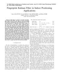
Figure 2.2: <strong>Doppler</strong> curve<br />
4
in Figure 2.2. The shape of the so called <strong>Doppler</strong> curve in Figure 2.2 can be used<br />
to estimate the distance to the tracked object as well as its velocity. Numerically<br />
this can be done <strong>with</strong> least squares curve fitting.<br />
The applications of the <strong>Doppler</strong> effect are by no means limited to acoustics.<br />
Perhaps the most used application of the <strong>Doppler</strong> effect is radar. The principle<br />
of <strong>Doppler</strong> radar is explained in [Janza et al., p. 410]. In addition to radars,<br />
the <strong>Doppler</strong> effect is also important in lidars (light detection and ranging). The<br />
workingprinciple of a lidar closely resembles that of a radar, but the lidar is<br />
used at optical frequencies [Post & Cupp]. <strong>Doppler</strong> lidars are mainly used in<br />
atmospheric measurements of small particles.<br />
Another important application is the laser <strong>Doppler</strong> anemometry. The use of<br />
laser <strong>Doppler</strong> anemometry (LDA) in fluid velocity field measurement is explained<br />
in [Tropea]. The method is also sometimes called laser <strong>Doppler</strong> velocimetry<br />
[Wang& Snyder]. Furthermore, <strong>Doppler</strong> ultrasound measurements are widely<br />
used in medicine. Blood flow velocity, for example, is an important measurable<br />
that can be measured <strong>with</strong> <strong>Doppler</strong> ultrasound [Bascom & Cobbold].<br />
2.2 History of <strong>Doppler</strong> Navigation<br />
The precedingsection showed that there are numerous applications in different<br />
fields that take advantage of the <strong>Doppler</strong> effect. The <strong>Doppler</strong> effect, by its nature,<br />
is ideally suited for velocity measurement. However, it has already for longbeen<br />
used in navigation. In this section, we will enlighten the history of satellite<br />
<strong>Doppler</strong> navigation.<br />
The idea of a satellite <strong>Doppler</strong> navigation system comes from Applied Physics<br />
Laboratory of the John Hopkins University, United States. The invention was<br />
made in 1958 and was publicised in 1960. The early development of the project<br />
and a proof of feasibility of satellite <strong>Doppler</strong> navigation was presented in<br />
[Guier & Weiffenbach]. The U.S. Navy Navigation Satellite System, alsoknown<br />
as Transit, was designed based on this idea. The system became operational<br />
in 1964. Details of the system were released in 1967 by the U.S. government.<br />
This was done in order to permit commercial manufacture and use of Transit<br />
navigation equipment.<br />
The Transit system provided intermittent position fix updates rather than continuous<br />
navigation information [Laurila, p. 463]. It consisted of satellites in circular,<br />
polar orbits about 1075 kilometres high. The receiver only needed to track one<br />
satellite to produce a navigation fix. In order to produce an accurate estimate,<br />
5
the receiver needed to collect measurement data over several minutes. The actual<br />
computation of the receiver position was based on the <strong>Doppler</strong> curve of a satellite<br />
pass. <strong>Doppler</strong> curves of satellites are flatter than in Figure 2.2. This is because<br />
they travel alongcircular orbits rather than straight lines. The position of the<br />
receiver was determined by curve fitting. The latitude and longitude estimates<br />
were optimised such that the computed <strong>Doppler</strong> curve fitted to the measured<br />
data. The computational details can be found in [Laurila, p. 474]. The accuracy<br />
of the Transit system was about half a kilometre.<br />
In order to compute the <strong>Doppler</strong> curves, one also needs to know the position<br />
and velocity vectors of the satellite. Thus, the Transit satellites transmitted<br />
binary data by phase modulation. This data is called ephemeris. One was able<br />
to compute the satellite position and velocity from the ephemeris. The Transit<br />
satellites transmitted continuous wave signals on two distinct frequencies, namely<br />
150 MHz and 400 MHz. The purpose of this was to eliminate the first order<br />
ionospheric refraction and receiver frequency measurement errors. The accuracy<br />
of the Transit system was about 100 meters for a stationary receiver, but was<br />
severely worse for a receiver in unknown motion [Laurila, p. 476]. According<br />
to [Parkinson & Spilker, p. 4], the Transit system is still operational, but new<br />
satellites are not beinglaunched.<br />
6
Chapter 3<br />
The Global <strong>Positioning</strong> System<br />
In this chapter we will introduce the Global <strong>Positioning</strong>System. Its history and<br />
general working principles will be covered. The accuracy considerations and the<br />
limitations of the system are also discussed in short.<br />
3.1 History<br />
The history of the Global <strong>Positioning</strong>System (<strong>GPS</strong>) can be said to begin from<br />
the year 1973. Until then, the U.S. Navy and the U.S. Air Forces had been<br />
studying navigation separately. But in 1973 a Joint Program Office was formed<br />
by the U.S. Department of Defence (DOD). The new system called <strong>GPS</strong> or<br />
NAVSTAR, was planned. The first prototype satellites were launched in 1978<br />
[Parkinson & Spilker, pp. 4-9]. The full operational capability was reached by<br />
the end of year 1994.<br />
Although the <strong>GPS</strong> has been a military project, it has been designed also for<br />
the civil use. In the beginning the U.S. military feared that the <strong>GPS</strong> could be<br />
effectively used by the enemy. A system called selective availability (SA) was<br />
created. This meant that there were two different signals, one for the public and<br />
one encrypted for the military only. The public signal was deliberately degraded<br />
such that the accuracy for the civil users was an order of magnitude worse than<br />
for the military.<br />
As late as in May 2000 the SA was finally turned to zero. Technically the SA<br />
may still be re-introduced in case a need for that arises. The reason for turning<br />
SA off is partially the economic boost it was thought to give. Partially the reason<br />
is, however, that the effects of the SA can be circumvented <strong>with</strong> the modern<br />
technology. The mentioned modern technology involves carrier smoothing and so<br />
called differential <strong>GPS</strong> (D<strong>GPS</strong>).<br />
7
Recently, a project similar to the <strong>GPS</strong> has also been launched in the Europe. The<br />
project is called Galileo. The Galileo satellite system is planned to be perfectly<br />
compatible to the <strong>GPS</strong>. This is a benefit, because the same receivers can use<br />
either or both of the systems. The main difference between Galileo and <strong>GPS</strong><br />
is that Galileo has not been planned to be used by the military. Galileo is a<br />
completely civil project, which is funded by the European Union and various<br />
European companies. The Galileo system is expected to be operational in 2008<br />
[ESA].<br />
3.2 The Basic Concepts<br />
3.2.1 Reference Coordinate Systems<br />
In every kind of navigation one needs some reference coordinate system. In <strong>GPS</strong><br />
this is an important issue, since the natural coordinate systems for the satellites’<br />
positions and for the receiver’s position are different.<br />
The Earth-centred inertial (ECI)coordinate system is particularly suitable for<br />
determiningthe orbits of the satellites [Kaplan, p. 23]. The origin of the ECI<br />
system is at the centre of mass of the Earth. The equations of motion of the <strong>GPS</strong><br />
satellites can be modelled as if the ECI system were unaccelerated.<br />
For the purposes of computingthe position of a <strong>GPS</strong> receiver, it is more convenient<br />
to use a coordinate system that rotates <strong>with</strong> the Earth. This coordinate<br />
system is called Earth-centred Earth-fixed (ECEF)system. A stationary receiver<br />
on the surface of the Earth is stationary also in the ECEF coordinate system.<br />
Thus, the natural coordinate system for the satellites is ECI and that for the<br />
receiver is ECEF. The normal procedure is to compute the satellite orbits in<br />
the ECI system and then transform them to the ECEF system. Thereafter, the<br />
receiver position is computed in the ECEF system. In this thesis, unless otherwise<br />
specified, all the given coordinates will be in the ECEF coordinate system.<br />
3.2.2 Range <strong>Positioning</strong><br />
<strong>GPS</strong> has been designed to be a time-of-arrival positioningsystem. This means<br />
that the receiver’s position is determined by measuringthe time that the <strong>GPS</strong><br />
signal uses to travel from the satellite to the receiver. With the knowledge that<br />
the signal travels <strong>with</strong> the speed of light c, the satellite-to-receiver range can<br />
be computed. When range measurements are simultaneously performed <strong>with</strong><br />
8
sufficiently many satellites, the receiver’s position can be solved. An example in<br />
two dimensions is shown in Figure 3.1.<br />
Satellite 1<br />
Receiver<br />
Satellite 3<br />
Satellite 2<br />
Figure 3.1: Principle of Range <strong>Positioning</strong><br />
When the user knows the positions of the satellites and the satellite-to-receiver<br />
distances, he can draw a picture similar to Figure 3.1. In three dimensions the<br />
circles around the satellites are naturally spheres. The radii of the spheres are<br />
the distances to the satellites measured by the receiver. The receiver position can<br />
be found from the intersection of the spheres.<br />
3.2.3 <strong>GPS</strong> Signal Structure<br />
The <strong>GPS</strong> satellites transmit two different signals. Coarse/acquisition (C/A) signal<br />
is transmitted at the frequency L1 (1575.42 MHz). The C/A signal is open to<br />
be used by everyone. The precision (P(Y)) signal is transmitted at the frequency<br />
L2 (1227.6 MHz). The P(Y) signal is encrypted and can be used only by the U.S.<br />
military. The <strong>GPS</strong> receivers are totally passive in the sense that they need not<br />
transmit anything. In order to conclude its position, the receiver only needs to<br />
listen to the frequency L1.<br />
The satellite carrier signals are binary phase shift key modulated <strong>with</strong> pseudorandom<br />
noise (PRN) codes. The modulation frequency is 1.023 MHz. The code<br />
repeats once in a millisecond. The PRN codes are binary sequences that appear<br />
to be noise but are actually deterministic. Determinism is naturally necessary<br />
because the receiver needs to demodulate the signal. The noise-like characteristic<br />
9
of the PRN codes is crucial because all the satellites transmit at the same frequency.<br />
The PRN codes are used to differentiate the satellite signals from each<br />
other. The PRN codes have been designed to have extremely low cross-correlation<br />
[<strong>GPS</strong> 1995]. With their wide spectra and low cross-correlations, the PRN codes<br />
are ideally suited for makingthe difference between the satellite signals. Systems<br />
like the <strong>GPS</strong>, which transmit different data at the same frequency, are called code<br />
division multiple access systems.<br />
The satellites transmit also navigation data which is modulated to the C/A signal<br />
at 50 Hz frequency. The navigation data is organised in superframes, frames and<br />
subframes. The superframes, frames and subframes last 12.5 minutes, 30 seconds<br />
and 6 seconds, respectively.<br />
The navigation message contains for example the ephemeris. The ephemeris is a<br />
set of time varyingparameters that are used to calculate the position and velocity<br />
of the satellite. The satellite positions can be computed accurately or approximated<br />
[Korvenoja & Piché]. The knowledge of satellite’s position is crucial for<br />
the positioning, as can be seen from the Figure 3.1. If the satellite position is<br />
biased, also the receiver position will be incorrectly determined. The ephemeris<br />
contains also some correction terms that pass the user information for example<br />
about the satellite clock drift.<br />
One of the most important things that the navigation data contains, is the time.<br />
The time in the navigation message is the time of transmission of the beginning<br />
of each subframe. Thus, the time information is sent in the navigation message<br />
once in 6 seconds.<br />
3.2.4 Pseudorange and Delta Range<br />
Above, the <strong>GPS</strong> was stated to be a time-of-arrival positioningsystem. The way<br />
to measure the propagation times of the signals is based on the PRN codes.<br />
The satellite PRN code is replicated in the receiver. Retardingthe replica code<br />
and performinga correlation process <strong>with</strong> the received signal yields △ti, the<br />
signal propagation time from the ith satellite. This can be obtained because the<br />
user knows both the time of the beginning of each subframe from the navigation<br />
message and the time of signal reception from the correlation process. The <strong>GPS</strong><br />
signals travel at the speed of light c. Thus, the satellite-to-user range can be<br />
computed <strong>with</strong><br />
ri − ru = c△ti<br />
(3.1)<br />
where ri is the satellite position vector, ru is the receiver position vector, c is the<br />
speed of light and △ti is the signal propagation time.<br />
10
The satellite signal is very accurate. However, the user clock is usually not<br />
synchronised <strong>with</strong> the satellite clocks. This makes the exact measurement of the<br />
range impossible. If the satellite clock is behind the system time, the measured<br />
range shorter than the real range and vice versa. The measured range is called<br />
pseudorange and can be modelled as<br />
ρi = c (△ti + tu) =ri − ru + ctu + ɛρi<br />
(3.2)<br />
where tu is the receiver clock bias and ɛρi is the measurement error. The true<br />
pseudorange is the pseudorange measurement <strong>with</strong> no error:<br />
ρTi = ri − ru + ctu<br />
(3.3)<br />
The other significant measurable in <strong>GPS</strong> positioning is the delta range, orthe<br />
time derivative of the pseudorange. Let us find out an expression for the true<br />
delta range by differentiating the equation 3.3:<br />
˙ρTi = dρTi<br />
dt<br />
= d<br />
dt (ri − ru + ctu) =(wi − wu) • ri − ru<br />
ri − ru + c ˙<br />
tu<br />
(3.4)<br />
where wi is the satellite velocity vector, wu is the receiver velocity vector and ˙<br />
tu<br />
is the receiver clock bias time derivative, or the receiver clock drift. More information<br />
about measuring pseudorange and delta range can be found in [Braasch].<br />
The delta range measurements are further discussed in Chapter 4 and Chapter 5.<br />
3.3 Pseudorange <strong>Positioning</strong><br />
3.3.1 Problem Formulation<br />
The <strong>GPS</strong> receivers calculate their positions in a process called pseudorange positioning.<br />
Assume that the receiver measures pseudoranges to n satellites simultaneously.<br />
We can write the equation 3.2 for all the satellites simultaneously. We<br />
achieve the followingsystem of equations:<br />
⎧<br />
ρ1 = r1 − ru + ctu<br />
⎪⎨ ρ2 = r2 − ru + ctu<br />
(3.5)<br />
⎪⎩<br />
.<br />
ρn = rn − ru + ctu<br />
All the pseudoranges ρi are known from the measurements and all the satellite<br />
position vectors ri are known from the navigation data. It remains to solve for<br />
the user position vector ru and the receiver clock bias tu. Since ru ∈ R 3 ,there<br />
are four unknowns to be solved for. Thus, one needs at least four independent<br />
11
equations in the system of equations 3.5. Physically this means pseudorange<br />
measurements from at least four different satellites at the same time. If there<br />
are more than four equations, the methods developed for solvingoverdetermined<br />
systems of equations may be applied.<br />
3.3.2 Solution Procedure<br />
There are numerous methods for solvingthe system of equations 3.5. Both closedform<br />
and iterative solutions have been extensively studied. A good overview of<br />
different methods is provided in [Korvenoja, pp. 31-50]. Here we will introduce<br />
the most commonly used method, namely the iterative least squares algorithm.<br />
For notational simplicity, let us denote the user position and time vector as<br />
n =[xuyu zu ctu] T where xu, yu, zu are the user x, y, z coordinates, respectively,<br />
c is the speed of light and tu is the user clock bias. Moreover, let us<br />
denote the estimated user position and time vector as ˆn = T ˆxu ˆyu ˆzu c ˆtu .The<br />
expected pseudorange is denoted by ˆρi and is the theoretical pseudorange calculated<br />
assuming n = ˆn. With the pseudorange model 3.2 one has the expected<br />
pseudorange as a function of ˆn<br />
ˆρi =ˆρi(ˆn) =ri − ˆru + c ˆtu<br />
(3.6)<br />
Usingthe vector notation, we have the pseudorange measurement vector ρ =<br />
[ρ1 ρ2 ... ρn] T and the expected pseudorange vector ˆρ =[ˆρ1 ˆρ2 ... ˆρn] T<br />
Usingthe first order Taylor series, one can approximate the theoretical pseudorange<br />
vector ˆρ at any point ˆn + △n:<br />
ˆρ (ˆn + △n) =ˆρ (ˆn)+ ∂ˆρ<br />
△n (3.7)<br />
∂ ˆn<br />
where n is the linearization point and △n is an arbitrary vector. Naturally, the<br />
approximation 3.7 is most accurate when △n is small.<br />
Obviously, the ultimate purpose of the algorithm is to find the receiver’s position.<br />
Thus, the user needs to find a correction term △n such that the theoretical<br />
pseudoranges match the measured ones. This can be achieved by setting the<br />
right hand side of the equation 3.7 to equal ρ:<br />
ˆρ (ˆn)+ ∂ˆρ<br />
△n = ρ (3.8)<br />
∂ ˆn<br />
Now the equation 3.8 can be solved. Accordingto [Kaplan, p. 521], the least<br />
squares solution for the correction term is<br />
△n = −<br />
∂ˆρ<br />
∂ ˆn<br />
T ∂ˆρ<br />
∂ ˆn<br />
12<br />
−1 T ∂ˆρ<br />
(ˆρ − ρ) (3.9)<br />
∂ ˆn
The estimated position and time vector ˆn can be updated by addingthe correction<br />
term △n to the estimate ˆn. Thereafter, the expected pseudorange vector ˆρ and<br />
the derivative matrix ∂ˆρ<br />
can be calculated again. This allows one to re-use<br />
∂ ˆn<br />
the equation 3.9 to find a new correction term △n. Thus, the iteration can<br />
be continued, until a satisfactory accuracy for the position and time estimate is<br />
reached.<br />
3.4 <strong>Positioning</strong> Error Analysis<br />
The precedingsection introduced an algorithm that is capable of findinga navigation<br />
solution. However, the navigation solution is not necessarily the same as<br />
the real receiver position and time. This results from measurement errors.<br />
It is highly desirable to be able to estimate the accuracy of the navigation solution,<br />
no matter which method is used. The standard method used in the <strong>GPS</strong><br />
pseudorange positioning will be introduced here. It appears that the derivative<br />
matrix ∂ˆρ<br />
∂ ˆn<br />
has an important role in error estimation. For simplicity, let us use<br />
the notation H = ∂ˆρ<br />
∂ˆρ<br />
. Note that some books operate <strong>with</strong> the matrix −<br />
∂ ˆn ∂ ˆn<br />
[Kaplan, p. 51], while others define the geometry matrix as ∂ˆρ<br />
likewedo. The<br />
∂ ˆn<br />
matrix H will here be called the pseudorange geometry matrix. The purpose<br />
of this is to distinguish the matrix from another geometry matrix which will be<br />
introduced later in this thesis.<br />
With the new notations, let us rewrite the expression for the correction term in<br />
the equation 3.9:<br />
△n = − H T H −1 H T (ˆρ − ρ) (3.10)<br />
Let us assume that the pseudorange measurements have errors that are uncorrelated<br />
and have equal variances σ2 ρ. Following[Parkinson & Spilker, p. 414], one<br />
achieves an expression for the positioningerror covariance matrix:<br />
cov(△n) =E △n△n T = σ 2 T −1<br />
ρ H H (3.11)<br />
The matrix H T H −1 is called geometrical dilution of precision matrix or GDOP<br />
matrix. It contains the information about the quality of the satellite geometry.<br />
If one has an estimate for the measurement error variance σ 2 ρ, one can calculate<br />
the positioningvariance cov(△n) <strong>with</strong> the help of the GDOP matrix.<br />
However, it is not very convenient to have the positioningerror as a form of<br />
4 × 4 covariance matrix cov(△n). Actually the matrix cov(△n) containsmuch<br />
information that is not always needed by the user. The effect of the satellite<br />
13
geometry can be reduced to a single real number. The geometrical dilution of<br />
precision value (GDOP) is defined as<br />
H <br />
T −1<br />
GDOP = trace H (3.12)<br />
where trace means the summation alongthe main diagonal of the matrix. The<br />
GDOP value can be used for estimatingthe magnitude of the positioningerror,<br />
as follows:<br />
(3.13)<br />
σn =GDOP× σρ<br />
where σn is a combined standard deviation of the solution x, y, z and ctu components,<br />
while σρ is the pseudorange measurement standard error. Besides of<br />
the GDOP, there are other useful values that can be computed from the GDOP<br />
matrix. These include position DOP, horizontal DOP, vertical DOP and time<br />
DOP [Parkinson & Spilker, p. 414].<br />
The pseudorange positioning error <strong>with</strong> a particular satellite geometry can be<br />
estimated <strong>with</strong> the formula 3.13. Accordingto [Kaplan, p. 262], the standard<br />
error σρ in pseudorange measurements is about 8 meters. According to [Kaplan,<br />
p. 270], the GDOP value is on average below 3. The equation 3.13 now shows<br />
that the positioningerror is usually below 25 meters. Thus, the positioning<br />
performance <strong>with</strong> the <strong>GPS</strong> pseudorange positioning is far better than <strong>with</strong> the<br />
Transit <strong>Doppler</strong> positioningsystem.<br />
3.5 Limitations of the <strong>GPS</strong><br />
In the previous section it was stated that the <strong>GPS</strong> has a very good positioning<br />
performance. The theory for the pseudorange positioning is well developed and<br />
relatively easy. Still, the <strong>GPS</strong> has its limitations. One of the most severe is the<br />
satellite availability. The standard <strong>GPS</strong> receivers need to measure pseudoranges<br />
to at least four satellites simultaneously, in order to solve for the position estimate.<br />
In theory, at least four satellites should be available nearly always nearly everywhere<br />
[Kaplan, p. 287]. In practise, however, there are problems. The problems<br />
usually arise in weak signal conditions. Sometimes the receiver should have<br />
many satellites in sight but there is some barrier that prevents the <strong>GPS</strong> signal<br />
from reachingthe receiver. This occurs frequently in urban areas and indoors<br />
[Syrjärinne, p. 22]. Usually the signal is received, but it is too much attenuated<br />
for the pseudorange positioning purposes.<br />
Recently, some effort has been put to resolve the satellite availability problem.<br />
Novel methods have been developed for enhancingthe positioningperformance<br />
14
in weak signal conditions. The key for the solution seems to be the assisted <strong>GPS</strong>.<br />
This means that the receiver gains some extra information, for example through<br />
a cellular network. This helps when the receiver has not been able to demodulate<br />
the navigation message from the attenuated <strong>GPS</strong> signal. With assis<strong>GPS</strong>, also<br />
the attenuated signals can be exploited in the positioning determination. More<br />
details about these methods can be found in [Syrjärinne] and [Sirola].<br />
15
Chapter 4<br />
<strong>Doppler</strong> <strong>Positioning</strong> <strong>with</strong> the<br />
<strong>GPS</strong><br />
In this chapter, the possibility of usingthe <strong>Doppler</strong> measurements in <strong>GPS</strong> will<br />
be discussed. The theory for positioningbased on simultaneous <strong>Doppler</strong> measurements<br />
will be developed. In addition, an iterative algorithm suitable for the<br />
positioningis presented.<br />
4.1 Need for <strong>Doppler</strong> <strong>Positioning</strong><br />
The Global <strong>Positioning</strong> System was developed for pseudorange positioning. There<br />
is no doubt that usingthe pseudorange measurements is the most accurate way<br />
to find a position estimate for the receiver. However, the end of the preceding<br />
chapter gave a glimpse of the difficulties that frequently arise in pseudorange<br />
positioning.<br />
Very often it happens, that there are several attenuated <strong>GPS</strong> satellite signals<br />
available. The signals are so noisy that the demodulation of the navigation message<br />
is impossible. Thus, the pseudorange measurements cannot be performed.<br />
However, the signals are sufficiently good so that the signals can be recognised<br />
accordingto the PRN codes. In addition, the received signal frequencies can be<br />
measured. The frequency differences are mainly caused by the <strong>Doppler</strong> effect. In<br />
this chapter it will be shown that the frequency shifts can be used for positioning<br />
<strong>with</strong>out knowledge of the pseudoranges. This kind of positioning will be referred<br />
to as <strong>GPS</strong> <strong>Doppler</strong> positioning.<br />
In pseudorange positioning the user needs to know the satellite positions. In<br />
<strong>GPS</strong> <strong>Doppler</strong> positioningthe same applies, but the user also needs to know the<br />
satellite velocities. The usual way to achieve this information is to demodulate the<br />
16
navigation message. Here, however, we assumed that the signals are so attenuated<br />
that this is impossible. The solution is the assisted <strong>GPS</strong>. We will assume that<br />
the satellite orbital parameters and the current time is received from somewhere<br />
out of the <strong>GPS</strong> system. Typically this means that the receiver is connected to a<br />
cellular network.<br />
It is evident that the ability to perform the positioningusingonly <strong>Doppler</strong> measurements<br />
would be of great use in many situations. Even if the positioning<br />
estimate would not be as accurate as in pseudorange positioning, the <strong>Doppler</strong><br />
positioningwould still make sense. As was written above, the pseudorange positioningis<br />
not always possible. More good news is that carryingout the <strong>Doppler</strong><br />
measurements does not require any hardware modifications to the receiver. Actually,<br />
the state of the art receivers are doingthe <strong>Doppler</strong> measurements all the<br />
time as a by-product of satellite tracking.<br />
4.2 Comparison between <strong>GPS</strong> and Transit<br />
In Chapter 2 the basic principles of the historical Transit <strong>Doppler</strong> positioning<br />
satellite system were enlightened. The Chapter 3, by contrast, introduced the<br />
modern <strong>GPS</strong> pseudorange positioning. There is no doubt that <strong>GPS</strong> pseudorange<br />
positioningis much more accurate than the Transit <strong>Doppler</strong> positioning. But let<br />
us now assume that the <strong>GPS</strong> is used in <strong>Doppler</strong> positioningmode. Naturally, before<br />
going on to designing algorithms for <strong>GPS</strong> <strong>Doppler</strong> positioning, it is desirable<br />
to know if the positioninghas any chances to succeed. We know that the Transit<br />
positioningwas possible <strong>with</strong> about 500 meters accuracy. Let us now compare<br />
Transit and <strong>GPS</strong> <strong>Doppler</strong> positioningto see if the <strong>GPS</strong> can be expected to beat<br />
the Transit.<br />
Let us first consider the bad sides of the <strong>GPS</strong> when compared to the Transit.<br />
First of all, the <strong>GPS</strong> only has one available civil frequency. In Transit there were<br />
two separate frequencies. This is a bigbenefit allowingthe user to eliminate<br />
all the first order errors in measurements. Thus, most of the atmospheric and<br />
receiver measurement errors can be eliminated in the Transit. In addition, the<br />
Transit satellites were at lower orbits and travelled at a higher velocity. This<br />
produces benefits in <strong>Doppler</strong> positioning, because the <strong>Doppler</strong> shifts are larger.<br />
Furthermore, the positioninggeometry is better when the satellites are at lower<br />
orbits. In other words, the positioningerror for the same <strong>Doppler</strong> measurement<br />
error is smaller for low orbit satellites [Hill].<br />
However, there are also good things in the <strong>GPS</strong> when compared to the Transit.<br />
The biggest advantage of using the <strong>GPS</strong> for <strong>Doppler</strong> positioning in stead of the<br />
Transit is the satellite availability. There are much more satellites in the <strong>GPS</strong>. In<br />
17
the Transit, the receiver was lucky to be able to track even one satellite. Most of<br />
the time there were no satellites in the view. On the contrary, there are usually<br />
several <strong>GPS</strong> satellites in the view at the same time. Even if the receiver is indoors,<br />
most of the <strong>GPS</strong> signals can be received, although attenuated. The high number<br />
of satellites allows a <strong>GPS</strong> receiver to have simultaneous <strong>Doppler</strong> measurements<br />
from several satellites. This is a huge increase in the amount of information that<br />
can be used for the positioning.<br />
In addition, the <strong>GPS</strong> frequency is much higher than the Transit frequencies.<br />
This is a benefit, because relative frequency measurement errors become smaller.<br />
Furthermore, the higher frequency causes smaller atmospheric errors. As a conclusion,<br />
it cannot be said which is better: the Transit or the <strong>GPS</strong> <strong>Doppler</strong> positioning.<br />
Both have their advantages and drawbacks. A summary of these is<br />
shown in Table 4.1. After all, one can say that the <strong>GPS</strong> <strong>Doppler</strong> positioning<br />
may well be of at least the same accuracy as the Transit. Thus, there is a reason<br />
for further <strong>GPS</strong> <strong>Doppler</strong> positioningresearch. More thorough positioningerror<br />
analysis will be provided in Chapter 5.<br />
Table 4.1: Comparison between <strong>GPS</strong> <strong>Doppler</strong> positioningand Transit<br />
<strong>GPS</strong> Transit<br />
+Better satellite availability +Two different frequencies<br />
+Higher frequency +Higher satellite velocities<br />
+Lower satellite orbits<br />
4.3 The Governing Equations<br />
Let us now begin to build a physical model for the <strong>GPS</strong> <strong>Doppler</strong> positioning. This<br />
will eventually lead to an algorithm, that can be used in position estimation.<br />
4.3.1 The <strong>Doppler</strong> Shift Equation<br />
The frequency of the received <strong>GPS</strong> signal differs from the frequency transmitted<br />
by the satellite. This easily measurable frequency offset is mainly due to the<br />
<strong>Doppler</strong> effect. The <strong>Doppler</strong> effect is caused by the relative motion of the transmittingsatellite<br />
<strong>with</strong> respect to the receiver. The <strong>Doppler</strong> Shift can be modelled<br />
<strong>with</strong> the dot product equation<br />
<br />
wi − wu<br />
Di = − •<br />
c<br />
ri<br />
<br />
− ru<br />
L1<br />
(4.1)<br />
ri − ru<br />
18
where wi is the satellite velocity, wu is the receiver velocity, c is the speed of<br />
light, ri is the satellite location, ru is the receiver location and L1 is the frequency<br />
transmitted by the satellite.<br />
The <strong>Doppler</strong> shift equation 4.1 can be modified to achieve a range rate equation.<br />
For notational simplicity let us define the satellite’s relative velocity <strong>with</strong> the<br />
followingequation:<br />
(4.2)<br />
vi = wi − wu<br />
After algebraic manipulation one obtains<br />
vi • ru − ri<br />
ru − ri<br />
= Dic<br />
L1<br />
(4.3)<br />
We notice that the left hand side of the equation 4.3 is the rate at which the<br />
satellite is approachingthe user. Thus, the equation can also be written as a<br />
range rate equation as<br />
− d<br />
dt ru − ri = Dic<br />
(4.4)<br />
Assume that the user knows the current time as well as his own velocity exactly,<br />
and that he has the valid ephemeris. Consequently he can calculate satellites’<br />
position vectors ri and relative velocities vi. Also assume that the receiver knows<br />
the speed of light constant c, the real transmitted frequency L1 and the real<br />
<strong>Doppler</strong> shift Di.<br />
With precedingassumptions, the only unknown in the equation 4.3 is the user<br />
position vector ru. Interpretingthe dot product geometrically <strong>with</strong> the formula<br />
a • b = a·b·cos ∠(a, b) and noticingthat the vector ru − ri<br />
is of unit<br />
ru − ri<br />
length, the equation 4.3 can be written as<br />
L1<br />
vi·cos α = Dic<br />
L1<br />
(4.5)<br />
where α = ∠(vi, ru − ri) is the angle between the relative satellite velocity vi<br />
and the satellite-to-user vector ru − ri. Solvingfor the angle α in the equation<br />
4.5 gives us<br />
<br />
Dic<br />
α = arccos<br />
(4.6)<br />
L1vi<br />
Thus the receiver must be located such that the satellite-to-user vector ru − ri<br />
forms an angle α <strong>with</strong> the satellite relative velocity vector vi. The possible<br />
receiver positions ru form a surface of a right circular cone whose vertex is at<br />
the satellite position ri. The cone is shown in Figure 4.1. The cone has a semiinfinite<br />
axis in the direction of the satellite velocity vi when the <strong>Doppler</strong> shift<br />
Di is positive and in the direction opposite to vi when Di is negative. The angle<br />
between the surface of the cone and the satellite relative velocity vector vi is<br />
19
Dic<br />
α = arccos . As a special case of equation 4.6 when the <strong>Doppler</strong> shift<br />
L1vi<br />
Di equals zero the receiver must be located on a plane that is orthogonal to vi<br />
and passes through ri.<br />
ru<br />
vi ✛<br />
α<br />
ri<br />
vi·cos α<br />
Figure 4.1: <strong>Doppler</strong> effect in satellite positioning<br />
If we had three ideal <strong>Doppler</strong> measurements, we could solve for the three unknowns,<br />
namely the user position vector ru =[xu yu zu] T . The user position<br />
would be found at the intersection of the three different cones defined by the<br />
equation 4.3. However, things are unfortunately not that simple. It is extremely<br />
difficult to measure the <strong>Doppler</strong> shift <strong>with</strong> the precision required for the positioning.<br />
4.3.2 The Clock Drift Error<br />
In order to accurately measure the frequency of a signal, one must have a very<br />
stable clock. The same applies also to accurately generating a desired frequency.<br />
Satellite frequency generation is based on a highly accurate free running atomic<br />
standard. The <strong>GPS</strong> control segment makes sure that the frequencies transmitted<br />
by the satellites are very close to the nominal frequency L1 and adds correction<br />
terms to the navigation messages when necessary [Kaplan, p. 50]. Thus, the<br />
error in the transmitted frequency causes little harm for the receiver.<br />
By contrast, the receiver very seldom has sufficiently good an oscillator to accurately<br />
estimate the <strong>Doppler</strong> shift of the received signal. Let us denote the time<br />
derivative of the receiver clock bias, the receiver clock drift, by˙tu. If˙tu is positive,<br />
20
the receiver clock is runningfast and if ˙tu is negative, it is running slow. The<br />
error △f in the estimate for the received frequency can be modelled as<br />
△f = −˙tuL1<br />
(4.7)<br />
It is important to notice that the error in the received frequency estimate in the<br />
equation 4.7 is independent of the received frequency. Moreover, it is constant<br />
in the sense that it has the same value for every signal if frequencies of multiple<br />
signals are measured at the same time instant. However, the clock drift is not<br />
generally constant in time.<br />
4.3.3 Mathematical Problem Formulation<br />
Let us denote the receiver’s estimate for the frequency of the received signal<br />
from the satellite i by fi. Modellingthe frequency offsets from the <strong>Doppler</strong> shift<br />
(equation 4.1) and the receiver clock drift (equation 4.7) we obtain a model for<br />
the total frequency offset:<br />
fi − L1 = Di + △f + ɛfi<br />
<br />
vi<br />
= −<br />
c • ri<br />
<br />
− ru<br />
L1 − ˙tuL1 + ɛfi<br />
ri − ru<br />
(4.8)<br />
where ɛfi is the unmodelled noise in the frequency measurement. Properties of<br />
the measurement noise will be covered in Chapter 5.<br />
Multiplyingthe equation 4.8 by − c<br />
L1 yields<br />
− fi − L1<br />
c = vi •<br />
L1<br />
ri − ru<br />
ri − ru + c˙tu<br />
ɛfic − (4.9)<br />
L1<br />
c<br />
Usingthe equation 3.4 and denotingɛ ˙ρi = −ɛfi the equation 4.8 can be rewritten<br />
L1<br />
as<br />
− fi − L1<br />
c =˙ρTi + ɛ ˙ρi<br />
(4.10)<br />
L1<br />
is the delta range measurement noise.<br />
where ˙ρTi is the true delta range and ɛ ˙ρi<br />
The delta range measurement ˙ρi is the true deltarange ˙ρTi disturbed by the noise<br />
ɛ ˙ρi :<br />
˙ρi =˙ρTi + ɛ ˙ρi<br />
(4.11)<br />
Combiningthe equations 4.10 and 4.11, one achieves the delta range measurement<br />
model:<br />
˙ρi = − fi − L1<br />
L1<br />
c (4.12)<br />
Analogously, combining the equations 3.4 and 4.11 yields the delta range physical<br />
model:<br />
˙ρi = vi • ri − ru<br />
ri − ru + c˙tu + ɛ ˙ρi<br />
(4.13)<br />
21
For notational simplicity let us denote c˙tu, the effect of user clock drift to the<br />
delta range measurement, by d. The new variable d has unit of velocity, that is<br />
m/s. The true delta range can now be written in the form<br />
˙ρTi = vi • ri − ru<br />
+ d (4.14)<br />
ri − ru<br />
Now approximate the true delta range ˙ρTi <strong>with</strong> the measured delta range ˙ρi. Using<br />
the equation 4.14 we obtain the followingequation <strong>with</strong> 4 unknowns, namely<br />
ru ∈ R3 and d ∈ R:<br />
vi • ri − ru<br />
ri − ru + d − ˙ρi = 0 (4.15)<br />
Assume we have simultaneous delta range measurements from n different satellites.<br />
Each measurement contributes one equation similar to 4.15. This yields us<br />
the system of equations for multiple satellite <strong>Doppler</strong> positioning:<br />
where<br />
⎧<br />
⎪⎨<br />
⎪⎩<br />
v1 • r1 − ru<br />
r1 − ru + d − ˙ρ1 =0<br />
v2 • r2 − ru<br />
r2 − ru + d − ˙ρ2 =0<br />
.<br />
vn • rn − ru<br />
rn − ru + d − ˙ρn =0<br />
• vi,i=1..n are the satellite relative velocity vectors, assumed known<br />
• ri,i=1..n are the satellite position vectors, assumed known<br />
• ˙ρi,i=1..n are the delta range measurements, assumed known<br />
• ru is the receiver position vector, unknown<br />
(4.16)<br />
• d is the receiver clock drift effect to the delta range measurement, unknown<br />
Thus, there are four unknowns, namely xu,yu,zu and d. To simplify notations,<br />
let us make the followingdefinition:<br />
Definition 1. The receiver position and drift vector<br />
x =<br />
ru<br />
d<br />
⎡<br />
<br />
⎢<br />
= ⎢<br />
⎣<br />
22<br />
xu<br />
yu<br />
zu<br />
d<br />
⎤<br />
⎥<br />
⎦ ∈ R4
Let us now turn into our main goal, namely solvingthe positioningproblem<br />
defined by the system of equations 4.16. There are many different approaches<br />
for solvingthe problem. These include symbolic methods, standard numerical<br />
methods and problem specific iterative methods. It should be both mathematically<br />
and physically clear that the system of equations 4.16 cannot be uniquely solved<br />
unless the number of satellites n ≥ 4.<br />
4.4 Symbolic Methods<br />
4.4.1 Solving the Receiver Position<br />
In pseudorange positioning there are several different ways to manipulate the<br />
set of equations 3.5 such that one obtains closed-form solutions. It is naturally<br />
beneficial to have a closed-form solution for a problem because then one needs<br />
not resort to numerical iteration. A closed-form solution also produces valuable<br />
geometrical insight into the problem. Different closed-form solutions for pseudorange<br />
positioning can be found for example from [Bancroft], [Fang], [Krause],<br />
[Leva], [Hoshen] and [Lundberg].<br />
Because of the success of the closed-form solutions in pseudorange positioning<br />
there is also hope that similar solutions could be found in delta range positioning.<br />
The system of equations 4.16, however, is far more complex than the pseudorange<br />
equations 3.5. Consequently, there are no common knowledge closed-form<br />
solutions for the delta range equations. The main reason for the additional complexity<br />
of the delta range equations <strong>with</strong> respect to the pseudorange equations is<br />
the influence of the satellites’ relative velocity vectors vi.<br />
4.4.2 Existence and Uniqueness Considerations<br />
Let us continue to consider the system of delta range equations 4.16. One cannot<br />
be sure that there exists a solution variables ru and d such that the equations<br />
hold. Actually, if n>4 and the measurements are noisy, it is almost sure that a<br />
solution does not exist. However, as we will see later in this chapter, satisfying<br />
all the equations accurately is not necessary for a good positioning estimate.<br />
Furthermore, we cannot be certain that there is only one pair of variables (ru,d)<br />
that satisfy the equations 4.16. Probably, provided that a solution exists, there<br />
are at least two solutions for the equations [Hill]. However, only one solution is<br />
near the Earth and the other can be excluded.<br />
23
4.5 Standard Numerical Methods<br />
In this section, a new algorithm is developed for the <strong>GPS</strong> <strong>Doppler</strong> positioning.<br />
The algorithm is based on well known ideas from the numerical analysis. However,<br />
the method has not earlier been applied to the <strong>GPS</strong> <strong>Doppler</strong> positioningproblem.<br />
4.5.1 Problem Formulation<br />
In the following, we will consider iterative methods that begin from an initial<br />
guess for the solution and continue to gradually enhance the estimate.<br />
Notation 1. The receiver position and drift estimate<br />
⎡ ⎤<br />
ˆxu<br />
<br />
ˆru ⎢ ˆyu ⎥<br />
ˆx =<br />
ˆd<br />
= ⎢ ⎥<br />
⎣ ˆzu ⎦ ∈ R4<br />
ˆd<br />
is the current estimate for the receiver position and drift vector x<br />
Notation 2. The delta range measurement vector<br />
˙ρ =[˙ρ1 ˙ρ2 ... ˙ρn] T<br />
is a vector formed of the delta range measurements from the n satellites used in<br />
the calculations.<br />
The equation 4.13 gives a physical model for the delta range measurements. Assumingthat<br />
the noise components ɛ ˙ρi are zero-mean gives rise to the following<br />
definition:<br />
Definition 2. The expected delta range vector<br />
⎡<br />
⎢<br />
ˆ˙ρ = ⎢<br />
⎣<br />
v1 • r1 − ˆru<br />
r1 − ˆru + ˆ d<br />
v2 • r2 − ˆru<br />
r2 − ˆru + ˆ d<br />
.<br />
vn • rn − ˆru<br />
rn − ˆru + ˆ d<br />
is the expected delta range measurement vector assuming the receiver to be located<br />
at ˆru and the clock drift to be ˆ d.<br />
The positioningsolution procedure should aim at findinga point ˆx such that<br />
the expected delta range measurement vector would be equal to the real delta<br />
range measurement vector, that is ˆ˙ρ = ˙ρ. In order to have the problem in a<br />
mathematically standard form we will define the followinghelpful function:<br />
24<br />
⎤<br />
⎥<br />
⎦
Definition 3. Delta range residuals function<br />
⎡<br />
⎢<br />
p(ˆx) =ˆ˙ρ − ˙ρ = ⎢<br />
⎣<br />
v1 • r1 − ˆru<br />
r1 − ˆru + ˆ d − ˙ρ1<br />
v2 • r2 − ˆru<br />
r2 − ˆru + ˆ d − ˙ρ2<br />
.<br />
vn • rn − ˆru<br />
rn − ˆru + ˆ d − ˙ρn<br />
is a vector valued function <strong>with</strong> the receiver position and drift estimate ˆx as an<br />
argument. The components of the vector function are the differences between<br />
the predicted delta ranges assuming x = ˆx and the measured delta ranges ˙ρi.<br />
p(ˆx) ∈ R n ,wheren is the number of satellites used in the calculations.<br />
From the system of equations 4.16 one immediately notices that if the estimate<br />
ˆx is equal to the real position and drift vector x then the value of the function<br />
p(ˆx) must be a zero vector. Thus our hope for findingthe real receiver position<br />
and drift vector x lies in findinga zero of the function p(ˆx). The problem can<br />
be formulated by the followingequation<br />
⎡<br />
⎢<br />
p(ˆx) = ⎢<br />
⎣<br />
4.5.2 The Newton Method<br />
v1 • r1 − ˆru<br />
r1 − ˆru + ˆ d − ˙ρ1<br />
v2 • r2 − ˆru<br />
r2 − ˆru + ˆ d − ˙ρ2<br />
.<br />
vn • rn − ˆru<br />
rn − ˆru + ˆ d − ˙ρn<br />
⎤<br />
⎥<br />
⎦<br />
⎤<br />
⎥ ⎡ ⎤<br />
⎥ 0<br />
⎥ ⎢<br />
⎥ ⎢ 0.<br />
⎥<br />
⎥ = ⎢ ⎥<br />
⎥ ⎣ ⎦<br />
⎥<br />
⎦ 0<br />
(4.17)<br />
As should be clear from Subsection 4.4.2, there is no guarantee that the system of<br />
equations 4.16 has only one solution. Consequently, the equation 4.17 may well<br />
have solutions other than ˆx = x. In the followingwe will assume that we have<br />
an initial guess x0 that is sufficiently close to the real position and drift vector x.<br />
Then our solution algorithm should converge to the correct zero of the function<br />
p(ˆx).<br />
Here we will use the Newton method to find the solution. The solution procedure<br />
is based on the idea of linearly approximatingthe nonlinear function<br />
[Kaleva2000, p. 25]. This has to be done because there are no general methods for<br />
directly solvinga nonlinear equation. The linear approximation is accurate only<br />
in a small neighbourhood of the linearization point. However, as the linearization<br />
procedure is repeated, the solution estimate becomes increasingly accurate. Let<br />
25
us approximate the delta range residuals function p(ˆx) by the first order Taylor<br />
series at the estimated point xk:<br />
p(xk + △x) ≈ p(xk)+ ∂p(ˆx)<br />
<br />
<br />
△x (4.18)<br />
∂ ˆx<br />
where △x is a vector whose norm is relatively small.<br />
ˆx=xk<br />
For simplicity, we will use the followingnotation for the derivative matrix:<br />
G(xk) ≡ ∂p(ˆx)<br />
<br />
<br />
<br />
∂ ˆx<br />
ˆx=xk<br />
Now the approximate solution for the equation p(xk + △x) =0 can be found by<br />
settingthe right hand side of the approximate equation 4.18 to zero and solving<br />
for △x. Thus△x needs to be solved from the equation<br />
p(xk)+G(xk)△x = 0 (4.19)<br />
Assumingthat measurements from four satellites are used in the calculations<br />
(p(ˆx) ∈ R 4 ) and that the derivative matrix G(xk) is nonsingular, we obtain the<br />
equation<br />
△x = −[G(xk)] −1 p(xk) (4.20)<br />
where △x = xk+1 − xk is the difference between the new and the old estimated<br />
position and drift vector.<br />
4.5.3 The Gauss-Newton Method<br />
It is not very practical to limit oneself to use only four satellites in the positioning.<br />
There is always some noise present in the delta range measurements ˙ρi. Consequently,<br />
it is usually unwise to discard any available data. The Newton method<br />
can be slightly modified so that it can be used for any number of satellites. We<br />
want to use the equation 4.17 we have derived. Now when we may have more<br />
than four satellites it is highly probable that the delta range residuals function<br />
p(ˆx) does not have a zero. Instead, we now seek the point for which p(ˆx) is<br />
closest to the zero point in the Euclidean norm sense.<br />
The problem of the equation 4.17 is first reformulated as a nonlinear least squares<br />
problem:<br />
min p(ˆx) 2 : ˆx ∈ R 4<br />
(4.21)<br />
It is easy to see that when the number of satellites n = 4, the equations 4.17<br />
and 4.21 produce the same result ˆx. The difference is that the latter can be<br />
used always when n ≥ 4. When the equation 4.21 is solved by the Gauss-Newton<br />
26
method [Fletcher, p. 110], [Kaleva1998, p. 92], the iteration step solution 4.20 is<br />
replaced by the more general<br />
<br />
△x = − [G(xk)] T −1 [G(xk)] [G(xk)] T p(xk) (4.22)<br />
One can easily see that if G(xk) is a square matrix (G(xk) ∈ R 4×4 ) then the<br />
equation 4.22 reduces to equation 4.20. Thus, the equation 4.22 can be used<br />
<strong>with</strong>out losinggenerality.<br />
We end up <strong>with</strong> the following algorithm for searching the zero of the delta range<br />
residuals function in the least squares sense:<br />
1. Decide the initial guess x0 for the position and drift vector.<br />
2. Given xk, calculate the delta range residuals function p(xk) andthederivative<br />
matrix G(xk).<br />
3. Calculate<br />
<br />
the correction term △x from the equation<br />
△x = − [G(xk)] T −1 [G(xk)] [G(xk)] T p(xk)<br />
4. Calculate the new estimate for position and drift vector <strong>with</strong><br />
xk+1 = xk + △x<br />
5. Continue from step 2 <strong>with</strong> the new estimate xk+1 until △x is less than<br />
the desired tolerance<br />
4.5.4 Calculating the Derivative Matrix<br />
As was seen in the precedingsubsection the derivative matrix of the delta range<br />
residuals function <strong>with</strong> respect to the estimated user position and drift vector is<br />
vital for the Gauss-Newton method. Now we will focus on the matrix G in a<br />
little more detail.<br />
Since G = ∂p(ˆx)<br />
, the matrix G has as many rows as the delta range residuals<br />
∂ ˆx<br />
function p(ˆx) and as many columns as the position and drift estimate ˆx. Thus<br />
G ∈ R n×4 ,wherenis the number of satellites used in the calculations.<br />
The matrix G is very important for us because it appears in the equation 4.18<br />
which is used to linearly approximate the delta range residuals function p(ˆx).<br />
27
Fortunately, findingthe matrix G by algebraic differentiation of the function<br />
p(ˆx) is quite straightforward. Let us consider the differentiation in detail:<br />
G = ∂p<br />
∂ ˆx =<br />
⎡<br />
⎢<br />
∂p ⎢<br />
= ⎢<br />
ˆru<br />
∂<br />
⎢<br />
ˆd<br />
⎢<br />
⎣<br />
∂p1<br />
∂ ˆru<br />
∂p1<br />
∂ ˆ ∂p2<br />
∂ ˆru<br />
d<br />
∂p2<br />
∂ ˆ .<br />
∂pn<br />
d<br />
.<br />
∂pn<br />
∂ ˆru ∂ ˆ ⎤<br />
⎥ ∈ R<br />
⎥<br />
⎦<br />
d<br />
n×4<br />
(4.23)<br />
where pi are the components of the vector function p. Usingthe Definition 3,<br />
one obtains an expression for a single component of the vector function p. This<br />
can be written as<br />
pi(ˆx) =vi • ri − ˆru<br />
ri − ˆru + ˆ d − ˙ρi<br />
(4.24)<br />
Differentiatingthe ith component of the delta range residuals function p(ˆx) partially<br />
<strong>with</strong> respect to the estimated receiver position ˆru yields<br />
∂pi<br />
∂ ˆru<br />
= ∂<br />
∂ ˆru<br />
<br />
vi • ri − ˆru<br />
ri − ˆru + ˆ d − ˙ρi<br />
<br />
(4.25)<br />
In equation 4.25 vi, ri, ˆ d and ρi are constants <strong>with</strong> respect to the estimated<br />
receiver position ˆru. Applyingthe formula (fg) ′ = f ′ g + fg ′ for differentiating<br />
products gives us<br />
∂pi<br />
∂ ˆru<br />
= vi • (ri − ˆru) ∂ 1<br />
∂ ˆru ri − ˆru +<br />
vT i ∂<br />
(ri − ˆru)<br />
ri − ˆru ∂ ˆru<br />
1<br />
= vi • (ri − ˆru)<br />
ri − ˆru 2<br />
(ri − ˆru) T<br />
ri − ˆru −<br />
vT i<br />
ri − ˆru I3×3<br />
<br />
vi<br />
=<br />
ri − ˆru • ri<br />
<br />
− ˆru ri − ˆru<br />
ri − ˆru ri − ˆru<br />
<br />
ri − ˆru<br />
−<br />
ri − ˆru • ri<br />
T − ˆru vi<br />
ri − ˆru ri − ˆru<br />
where I3×3 is 3 × 3 identity matrix.<br />
(4.26)<br />
The equation 4.26 gives the partial derivative of the delta range residuals function<br />
<strong>with</strong> respect to the receiver position estimate. The form of the equation is<br />
satisfactory for numerical computation. However, the form is not very intuitive.<br />
The right hand side of the equation 4.26 can be transformed into a geometrically<br />
more illustrative form involvingcross products. Makinguse of the vector triple<br />
28
product formula a × (b × c) =(a• c)b − (a • b)c <strong>with</strong> a = c = ri − ˆru<br />
ri − ˆru and<br />
vi<br />
b = − gives us<br />
ri − ˆru<br />
∂pi(ˆx)<br />
∂ ˆru<br />
<br />
ri − ˆru<br />
=<br />
ri − ˆru ×<br />
<br />
−vi<br />
ri − ˆru × ri − ˆru<br />
ri − ˆru<br />
<br />
ri − ˆru<br />
=<br />
ri − ˆru ×<br />
<br />
ri − ˆru<br />
ri − ˆru ×<br />
vi<br />
ri − ˆru<br />
T<br />
T<br />
(4.27)<br />
The cross product of two vectors is always orthogonal to both vectors. Thus<br />
the partial derivative ∂pi<br />
lies in the same plane <strong>with</strong> both the satellite relative<br />
∂ ˆru<br />
velocity vector vi and the estimated receiver-to-satellite vector ri− ˆru. Moreover,<br />
∂pi<br />
is perpendicular to ri − ˆru. Figure 4.2 illustrates the situation. The negative<br />
∂ ˆru<br />
of the derivative vector is presented in the figure for graphical clarity.<br />
ru<br />
ri − ru✯<br />
ri<br />
−<br />
<br />
❄<br />
vi<br />
ri − ˆru<br />
∂pi(ˆx)<br />
∂ ˆru<br />
Figure 4.2: Derivative of the delta range difference function<br />
To complete the symbolical calculation of the derivative matrix G we still need<br />
to find the partial derivative of the delta range residuals function <strong>with</strong> respect to<br />
the clock drift estimate. Fortunately, this problem is trivial. One can easily see<br />
from the equation 4.24 that ∂pi(ˆx)<br />
∂ ˆ = 1. Now we know all the necessary partial<br />
d<br />
derivatives of the components of the delta range residuals function in order to<br />
form the matrix G in equation 4.23:<br />
⎡ <br />
r1 − ˆru<br />
⎢ r1 − ˆru<br />
⎢<br />
G(ˆx) = ⎢<br />
⎣<br />
×<br />
<br />
r1 − ˆru<br />
r1 − ˆru ×<br />
T v1<br />
r1 − ˆru<br />
<br />
r2 − ˆru<br />
r2 − ˆru ×<br />
<br />
r2 − ˆru<br />
r2 − ˆru ×<br />
T v2<br />
r2 − ˆru<br />
.<br />
<br />
rn − ˆru<br />
rn − ˆru ×<br />
<br />
rn − ˆru<br />
rn − ˆru ×<br />
T vn<br />
rn − ˆru<br />
29<br />
1<br />
1<br />
.<br />
1<br />
⎤<br />
⎥<br />
⎦<br />
(4.28)
The matrix G(x), that is the derivative matrix calculated at the true position<br />
and drift point x, is called <strong>Doppler</strong> geometry matrix. Sometimes the <strong>Doppler</strong><br />
geometry matrix G(x) will be written <strong>with</strong>out the argument as G.<br />
4.6 Problem Specific Iterative Methods<br />
It would appear that the first algorithm for <strong>GPS</strong> <strong>Doppler</strong> positioning was invented<br />
by Jonathan Hill. In his paper [Hill], presented in ION <strong>GPS</strong> 2001, he discusses the<br />
feasibility of <strong>Doppler</strong> positioning. He describes an iterative algorithm that uses<br />
least squares technique after an algebraic manipulation of the set of equations<br />
4.16.<br />
The Hill algorithm does not use the derivative matrix G at all. This has the<br />
advantage of somewhat lighter computation. On the other hand, the derivative<br />
matrix could be beneficial when analysingthe positioningerror, as will be shown<br />
in the followingchapter. There is no documented testingof the convergence<br />
properties of the Hill algorithm.<br />
Probably other iterative algorithms suitable for <strong>Doppler</strong> positioning can be found.<br />
Decidingwhich algorithm to use requires extensive numerical testingand depends<br />
on user’s needs. At least computational efficiency, reliability, convergence properties<br />
and error estimation have to be considered when choosingthe algorithm.<br />
30
Chapter 5<br />
<strong>Positioning</strong> Performance<br />
In the precedingchapter, it was shown that the receiver position can be estimated<br />
usingonly the delta range measurements <strong>with</strong> the current ephemeris and time.<br />
If the <strong>Doppler</strong> shift in the received frequency could be measured precisely, one<br />
would achieve the accurate position. Unfortunately, there is always some noise<br />
present in the measurements. In this chapter, we will discuss positioningaccuracy<br />
for <strong>GPS</strong> <strong>Doppler</strong> positioningand consider the things that affect it.<br />
5.1 Measurement Noise<br />
Theoretical analysis of the measurement noise is extremely difficult. This is<br />
because the sources of the errors are numerous and depend on the receiver architecture<br />
as well as many other conditions. In this chapter we will only introduce<br />
the main error sources and give some order of magnitude estimates for them.<br />
The more detailed statistical properties of the measurement noise need to be determined<br />
<strong>with</strong> the help of measurement data. Some examples will be given in<br />
Chapter 6.<br />
There are several sources of errors in <strong>GPS</strong> <strong>Doppler</strong> positioning. In the following,<br />
we will discuss the ionospheric effects, receiver noise, the effect of unknown user<br />
velocity and the effect of biased time estimate.<br />
5.1.1 Ionospheric Effects<br />
The <strong>GPS</strong> signals are electromagnetic waves that travel at the speed of light in<br />
vacuum. However, as a signal arrives to the ionosphere, its speed is slowed<br />
down by ions. This causes errors both to pseudorange and delta range measurements.<br />
In delta range measurements, the error due to the ionosphere is<br />
31
proportional to the rate of change of the total electron content of the ionosphere.<br />
The upper limit for the frequency measurement error due to the ionosphere is<br />
0.085 Hz. This value corresponds to the error of 1.6 cm/s in the delta range<br />
measurement[Parkinson & Spilker, p. 495].<br />
The frequency shift due to the ionosphere is a function of transmitted frequency.<br />
Consequently, the users receivingtwo different frequencies can correct for the first<br />
order ionospheric errors.<br />
5.1.2 Receiver Noise<br />
Even if the frequency of the <strong>GPS</strong> signal managed to penetrate the ionosphere<br />
<strong>with</strong>out disturbance, the actual measurement would still cause errors. The properties<br />
of the measurement errors depend heavily on the receiver architecture. The<br />
largest receiver error in the frequency measurement is the clock drift error d. Its<br />
effect on the delta range measurement can be of the order of 10 m/s. Fortunately,<br />
the clock drift error can be taken as an extra variable that is solved for, as was<br />
done in Chapter 4. The order of magnitude of the remaining receiver noise is<br />
hard to estimate theoretically.<br />
5.1.3 Unknown User Velocity<br />
In Subsection 4.3.3 we assumed that the satellite relative velocity vectors vi are<br />
known. With the equation 4.2, vi was defined as wi − wu, wherewi is the<br />
satellite velocity vector and wu is the user velocity vector. The satellite velocity<br />
vector wi can be calculated from the current ephemeris if one knows the current<br />
time. By contrast, the user velocity vector wu is unknown unless one has some<br />
extra information. The most common form of extra information is probably the<br />
knowledge that the user is stationary.<br />
Takingthe vector wu as a variable to be solved for means that we have three<br />
more unknowns, since wu ∈ R 3 . Thus, the number of required satellites for the<br />
positioningincreases from four to the usually unrealistic number of seven. Solving<br />
for wu is not considered any further here.<br />
Let us consider the error that the unknown user velocity causes. Assume that<br />
the user velocity wu is replaced by a biased user velocity estimate wu + △wu.<br />
Then, accordingto the equation 4.2, the satellite relative velocity vectors vi are<br />
32
eplaced by vi −△wu. Let us rewrite the equations 4.24 and 4.13 here for the<br />
simplicity of reference:<br />
pi(ˆx) =vi • ri − ˆru<br />
ri − ˆru + ˆ d − ˙ρi<br />
(5.1)<br />
˙ρi = vi • ri − ru<br />
ri − ru + c˙tu + ɛ ˙ρi<br />
(5.2)<br />
From the equation 5.2, one sees that the ith component of the delta range residuals<br />
function, pi(ˆx), is replaced by pi(ˆx) −△wu • ri − ˆru<br />
. Usingthe equations 5.1<br />
ri − ˆru<br />
and 5.2, one finally notices that error △wu in the user velocity is equivalent<br />
to additional error in the delta range measurement. Thus, the errors in the<br />
user velocity estimate can be analysed similarly to the errors in the frequency<br />
measurement. If the only error present is the error in the user velocity estimate,<br />
we have<br />
ɛ ˙ρi = △wu • ri − ˆru<br />
ri − ˆru<br />
(5.3)<br />
Furthermore, let us assume that the user position estimate ˆru is close to the real<br />
user position ru. Now the unit vector ri − ˆru<br />
ri − ˆru can be replaced by ri − ru<br />
ri − ru .<br />
Finally, we get the equation for the effect to the measurement:<br />
△wu • ri − ru<br />
ri − ru<br />
ru<br />
❥<br />
△wu<br />
ɛ ˙ρi = △wu • ri − ru<br />
ri − ru<br />
✿<br />
ru − ri<br />
Figure 5.1: Delta range measurement error caused by user velocity<br />
ri<br />
(5.4)<br />
Figure 5.1 shows the situation graphically. It is evident that the unknown user<br />
velocity has most effect to the measurement when its direction is alongthe line-ofsight<br />
vector. On the contrary, the effect is zero if the unknown user velocity vector<br />
is perpendicular to the line-of-sight vector. Usually, any direction of unknown<br />
user velocity cannot be ruled out. Thus, the worst case situation is that the<br />
effect to the delta range measurements is the speed of the receiver, or △wu.<br />
Apparently, even very slow velocities may have drastic effects on the positioning<br />
accuracy. In the above it was stated that the ionospheric errors are not larger<br />
that 1.6 cm/s. Now, if the receiver is experiencingan unknown motion of, say<br />
1.6 m/s, the measurement error level would effectively be 100 times larger.<br />
33
More bad news is that the user velocity is extremely hard to measure. A speedometer<br />
will not do, since it produces no information about the direction of the<br />
velocity. And even if the user velocity vector could be determined, say <strong>with</strong> a<br />
combination of gyroscopes and three-dimensional compasses, transforming the<br />
vector into the ECEF coordinate system would complicate the computation.<br />
5.1.4 Biased Time Estimate<br />
In Chapter 4 we assumed that the ephemeris and an accurate time estimate were<br />
available. In practise, however, the receiver only has an estimate for the current<br />
time. In conditions where pseudorange measurements are unavailable the <strong>GPS</strong><br />
satellites cannot provide time information. Thus, the receiver time estimate is<br />
probably biased. The consequence of the biased time estimate is that the satellite<br />
positions and velocities are calculated wrong.<br />
The biased time estimate effect can again be thought of as a measurement error.<br />
The positioning algorithms utilise the delta range difference function p(ˆx).<br />
Accordingto Definition 3, we have<br />
p(ˆx) =ˆ˙ρ − ˙ρ (5.5)<br />
Evidently, the biased time estimate causes error to the expected delta range vector<br />
ˆ˙ρ. Accordingto the equation 5.5, however, the effect is the same as if there were<br />
additional error in the delta range measurement vector ˙ρ. The resultingerror can<br />
be accurately approximated by examiningthe differences of the expected delta<br />
range vectors at time t and at the biased time t + △t. When△t is small we can<br />
use the first order Taylor series:<br />
ˆ˙ρ(t + △t) − ˆ˙ρ(t) = ∂ ˆ˙ρ △t (5.6)<br />
∂t<br />
The symbolic differentiation of the i th component gives<br />
∂ ˆ˙ ρi<br />
∂t = ri − ru<br />
ri − ru3 • vi × (ri − ru × vi)+ri − ru 2 <br />
ai<br />
(5.7)<br />
where ai is the relative acceleration vector of the i th satellite. Theoretical bounds<br />
<br />
<br />
∂<br />
ˆ˙ρi<br />
<br />
<br />
for are hard to derive from the equation 5.7. This is because the two vectors<br />
∂t <br />
in the square brackets are pointingto nearly opposite directions. Numerical<br />
<br />
∂<br />
ˆ˙ρi<br />
<br />
<br />
simulations show that the maximum value of <br />
∂t is about 15 cm/s2 . Applying<br />
the equation 5.6, wee see that for example a time bias error of 0.1 seconds may in<br />
the worst case cause a positioningerror similar to 1.5 cm/s measurement error.<br />
34
Thus, the time bias effect to the positioningaccuracy may easily be at least the<br />
same order of magnitude as the ionospheric errors.<br />
A solution for the time bias error might be iterating the time estimate. If the<br />
time estimate is expected to be too much biased, one could take it as an unknown<br />
variable and solve it. This results in an additional column to the <strong>Doppler</strong><br />
geometry matrix G. The components of the column would be of the form of the<br />
right hand side of the equation 5.7. This would also mean that a fifth satellite is<br />
needed to produce more measurement information.<br />
5.2 <strong>Positioning</strong> Accuracy<br />
5.2.1 Effect of Measurement Errors on <strong>Positioning</strong> Solution<br />
Let us now discuss the effect of the measurement noise on the position estimate.<br />
In the following, we will consider the accuracy of the Gauss-Newton method.<br />
Since the Gauss-Newton method is iterative, its error estimates are very difficult<br />
to derive rigorously. However, <strong>with</strong> the help of a few simplifying assumptions this<br />
can be done.<br />
Let us assume that the initial guess is sufficiently close to the real receiver coordinates<br />
so that the Newton method converges towards the right minimum. Consider<br />
the algorithm for positioning presented in Section 4.5.2. Now focus on the last<br />
step of the iterative algorithm. The last step takes place just before ending criterion<br />
is fulfilled. Accordingto the formula 4.22, the ultimate estimate ˆx for the<br />
receiver position and drift vector is calculated from<br />
ˆx = xk − [G(xk)] T [G(xk)] −1 [G(xk)] T p(xk) (5.8)<br />
Accordingto the Definition 3, we have p(ˆx) =ˆ˙ρ − ˙ρ. The delta range measurement<br />
vector ˙ρ can in turn be presented as a sum of the true delta range vector<br />
˙ρ T and the measurement error vector ɛ ˙ρ as<br />
˙ρ = ˙ρ T + ɛ ˙ρ<br />
(5.9)<br />
Correspondingly, the position and drift estimate ˆx can be presented as a sum of<br />
the true position and time x and the positioningerror ɛx:<br />
ˆx = x + ɛx<br />
Thus, the equation 5.8 can be written as<br />
x − xk + ɛx = [G(xk)] T [G(xk)] −1 [G(xk)] T<br />
<br />
35<br />
˙ρ T − ˆ˙ρ + ɛ ˙ρ<br />
<br />
(5.10)<br />
(5.11)
If the measurements and other data were ideal, the positioningsolution would<br />
also be perfect. Thus setting ɛ ˙ρ = 0 indicates that ɛx = 0. Applyingthese for<br />
the equation 5.11 gives us<br />
x − xk = [G(xk)] T [G(xk)] −1 [G(xk)] T<br />
<br />
˙ρ T − ˆ˙ρ (5.12)<br />
Now subtractingthe equation 5.12 from the equation 5.11 yields<br />
ɛx = [G(xk)] T [G(xk)] −1 [G(xk)] T ɛ ˙ρ<br />
(5.13)<br />
Let us simplify things by assuming the last linearization point xk to be very close<br />
to the true position and drift x. Now the matrix G(xk) can be approximated<br />
by the <strong>Doppler</strong> geometry matrix G(x), which will be denoted G. Finally, we<br />
have an equation that approximates the effect of the measurement errors on the<br />
positioningsolution:<br />
ɛx = G T G −1 T<br />
G ɛ ˙ρ<br />
(5.14)<br />
5.2.2 <strong>Doppler</strong> Dilution of Precision<br />
The equation 5.14 can be used to calculate the error in the positioningestimate<br />
if the measurement error ɛ ˙ρ is known. Unfortunately, ɛ ˙ρ can never be known. If<br />
the error was known it could be compensated and there would be no error at all.<br />
However, one should thrive to achieve an estimate for the accuracy of the solution.<br />
Otherwise, the user cannot really trust that the solution is even near the right<br />
one. The positioningerror can be estimated by statistical methods. For that<br />
we need some knowledge or assumptions about the statistical properties of the<br />
measurement error ɛ ˙ρ. Letusassume the following:<br />
• The measurement errors are zero mean, that is their expected values are<br />
zero:<br />
E {ɛ ˙ρ} = 0 (5.15)<br />
• The measurements from different satellites have uncorrelated errors and<br />
equal variances σ 2 ˙ρ:<br />
cov(ɛ ˙ρ) =E ɛ ˙ρɛ ˙ρ T = σ 2 ⎢<br />
˙ρIn×n = ⎢<br />
⎣<br />
36<br />
⎡<br />
σ2 ˙ρ 0 ··· 0<br />
0 σ2 ˙ρ ··· 0<br />
.<br />
.<br />
...<br />
0 0 ··· σ 2 ˙ρ<br />
.<br />
⎤<br />
⎥<br />
⎦<br />
(5.16)
Let us first calculate the expected value of the positioningerror. According<br />
to elementary statistics the expectation operator E is linear. Manipulatingthe<br />
equation 5.14 we obtain<br />
E {ɛx} =<br />
G <br />
T −1 T<br />
E G G ɛ ˙ρ = G T G =<br />
T −1 T<br />
G G G 0 =<br />
−1 T<br />
G E(ɛ ˙ρ)<br />
0<br />
(5.17)<br />
The equation 5.17 does not mean that the positioningerror would always be<br />
zero. It simply indicates that the errors of the xu, yu, zu and d components have<br />
equal probability of beingeither negative or positive. To achieve more useful<br />
information about the magnitude of the positioning error one needs to calculate<br />
a second order statistical number, namely the covariance:<br />
<br />
<br />
T<br />
cov(ɛx) = E (ɛx − E {ɛx})(ɛx − E {ɛx})<br />
eq.5.17<br />
<br />
=<br />
<br />
E ɛxɛT eq.5.14<br />
<br />
=<br />
=<br />
<br />
x<br />
G <br />
T −1 G <br />
T T −1<br />
T<br />
T<br />
E G G ɛ ˙ρ G G ɛ ˙ρ<br />
<br />
G T −1 T<br />
E G G ɛ ˙ρɛ ˙ρ T =<br />
G <br />
T −1<br />
T<br />
G G<br />
G T −1 T<br />
E G G ɛ ˙ρɛ ˙ρ T G G T G −1 <br />
=<br />
G T G −1 T<br />
G E ɛ ˙ρɛ ˙ρ T G G T G −1 eq.5.16<br />
<br />
=<br />
T −1 T 2 G G G σ ˙ρIn×nG G T G =<br />
−1<br />
G T G −1 2 σ ˙ρ<br />
(5.18)<br />
The result is completely analogous to the pseudorange positioning error analysis<br />
[Kaplan, p. 262]. The matrix G T G −1 in the equation 5.18 is very important to<br />
us and deserves an own name:<br />
Definition 4. The <strong>Doppler</strong> geometrical dilution of precision (DGDOP)matrix<br />
A = G T G −1<br />
The equation 5.18 shows us how the positioningaccuracy is dependent on the<br />
DGDOP matrix A. One has to keep in mind that the result was derived using<br />
the very strongassumptions 5.15 and 5.20.<br />
Thus the effect of satellite geometry on the positioning performance can be presented<br />
as a matrix A ∈ R 4×4 . This is considerable reduction of information<br />
since the satellite geometry is dependent on several vectors, namely the receiver<br />
position, satellite positions and satellite velocities. However, the matrix A still<br />
37
contains 16 components whose meaningneeds to be clarified. The matrix A in<br />
its component form can be presented as follows:<br />
⎡<br />
⎤<br />
A =<br />
⎢<br />
⎣<br />
A11 A12 A13 A14<br />
A21 A22 A23 A24<br />
A31 A32 A33 A34<br />
A41 A42 A43 A44<br />
⎥<br />
⎦<br />
(5.19)<br />
The covariance of the positioningestimate can in turn be presented as follows:<br />
⎡<br />
⎤<br />
cov(ɛx) =<br />
⎢<br />
⎣<br />
σ 2 xu σ 2 xuyu σ2 xuzu σ2 xud<br />
σ 2 xuyu σ 2 yu σ 2 yuzu σ2 yud<br />
σ 2 xuzu σ2 yuzu σ 2 zu σ 2 zud<br />
σ 2 xud σ 2 yud σ 2 zud σ 2 d<br />
⎥<br />
⎦<br />
(5.20)<br />
What really interests us are the variances σ2 xu , σ2 yu , σ2 zu and σ2 d . Using5.18, 5.19<br />
and 5.20 one obtains expressions for the precedingvariances:<br />
σ 2 xu = A11 × σ 2 ˙ρ (5.21)<br />
σ 2 yu = A22 × σ 2 ˙ρ (5.22)<br />
σ 2 zu = A33 × σ 2 ˙ρ (5.23)<br />
σ 2 d = A44 × σ 2 ˙ρ (5.24)<br />
When evaluatingpositioningperformance it is more natural to use standard deviations<br />
σ rather than variances σ 2 because standard deviations are physically<br />
much more intuitive. Mathematically transformingbetween the two does not<br />
cause any problems since the standard deviation is naturally the square root of<br />
the variance. Usingthe ratios of different positioningaccuracy standard deviations<br />
and the measurement accuracy standard deviation we can define <strong>Doppler</strong><br />
dilution of precision (<strong>Doppler</strong> DOP, DDOP) measures. These measures indicate<br />
the quality of the positioninggeometry. They are defined as follows:<br />
• <strong>Doppler</strong> position dilution of precision (DPDOP)<br />
<br />
σ2 xu + σ2 yu + σ2 zu<br />
= DPDOP =<br />
σ ˙ρ<br />
A11 + A22 + A33<br />
• <strong>Doppler</strong> horizontal dilution of precision (DHDOP)<br />
<br />
σ2 xu + σ2 yu<br />
= DHDOP =<br />
σ ˙ρ<br />
A11 + A22<br />
• <strong>Doppler</strong> vertical dilution of precision (DVDOP)<br />
<br />
σ2 zu<br />
= DVDOP =<br />
σ ˙ρ<br />
A33<br />
38<br />
(5.25)<br />
(5.26)<br />
(5.27)
• <strong>Doppler</strong> drift dilution of precision (DDDOP)<br />
<br />
2 σd = DDDOP =<br />
σ ˙ρ<br />
A44<br />
(5.28)<br />
The definitions 5.25–5.28 are completely analogous to the pseudorange positioning<br />
dilution of precision measures [Parkinson & Spilker, p.414], [Kaplan, p.268]. The<br />
only difference is that there is no natural way of defininga combined dilution<br />
measure for both position and drift. This measure is called geometric dilution<br />
of precision in pseudorange positioning. The lack of this measure in <strong>Doppler</strong><br />
positioningis caused by the fact that the unit of position is meters whereas the<br />
unit of the drift equivalent is meters per second. Obviously, variables of different<br />
units cannot be summed up. The problem could be circumvented by scaling<br />
the drift equivalent d in an appropriate way. However, there is no physically<br />
intuitive way of expressingthe drift in units of length. After all, one is usually<br />
only interested in the positioningaccuracy, not the accuracy of the drift estimate.<br />
Thus, there is no actual need for a unified dilution measure.<br />
5.2.3 Applications of the <strong>Doppler</strong> Dilution of Precision<br />
Concept<br />
In the precedingsubsection, we defined different DDOP measures. Here we will<br />
consider what they can be used for.<br />
We still need to keep in mind the assumption 5.16 on measurement errors, which<br />
are uncorrelated and have the same variances. With this assumption, we were<br />
able to derive the equations 5.25–5.28. Now these equations can be used to<br />
estimate the positioningerror. It is easy to see that the followingequations hold:<br />
<br />
σ 2 xu + σ2 yu + σ2 zu =DPDOP× σ ˙ρ<br />
<br />
σ 2 xu + σ2 yu =DHDOP× σ ˙ρ<br />
(5.29)<br />
(5.30)<br />
σzu =DVDOP× σ ˙ρ<br />
(5.31)<br />
σd = DDDOP × σ ˙ρ<br />
(5.32)<br />
The <strong>Doppler</strong> dilution of precision values are relatively easy to compute. Now if we<br />
have an estimate for the delta range measurement standard error σ ˙ρ we can easily<br />
achieve estimates for the position estimate standard deviation usingthe equations<br />
5.29–5.32. Estimate for the positioningerror is naturally of great value. The<br />
position estimate achieved by usingthe algorithm presented in Subsection 4.5.2<br />
would be of little value if its error could not be estimated.<br />
39
The DDOP concept is extremely beneficial both theoretically and practically. It<br />
allows one to consider the positioningerror as a product of two independent factors,<br />
namely the delta range measurement error and the quality of the satellite<br />
constellation. If the measurement standard error can be estimated then the positioningstandard<br />
error can also be estimated theoretically <strong>with</strong>out numerical<br />
simulation or buildinga positioningapparatus. This is important when assessing<br />
the performance of <strong>Doppler</strong> positioningbecause <strong>GPS</strong> <strong>Doppler</strong> positioningapparatuses<br />
are not even known to exist. Theoretical analysis is also in many ways<br />
more reliable than experimenting<strong>with</strong> real hardware. In the latter, the effects<br />
of the measurement errors cannot be separated from the effect of the satellite<br />
constellation. Of course, all this applies only if our assumptions on the nature of<br />
the measurement errors are valid.<br />
Another benefit of the <strong>Doppler</strong> dilution of precision concept is the qualitative<br />
information it gives. Different satellite geometries can easily be compared and<br />
the user can be informed when the DDOP measures are high and the results are<br />
not reliable. Usingthe DDOP values, one can also easily select the best visible<br />
satellites. Usingonly part of the satellites in computations reduces computational<br />
costs and power consumption. When usingall the visible satellites, the DDOP<br />
values are always on their lowest. Sometimes, however, the user does not want<br />
to use all the satellites but selects only a smaller amount of them. This could<br />
be for example in order to avoid the heavy computations needed to process all<br />
the visible satellites. The DDOP values are of great importance in this kind of<br />
situations. The difference between the positioningerrors when usingthe four<br />
best satellites and when usingthe four worst satellites could be several orders of<br />
magnitude.<br />
The probability distribution of the DDOP values is almost impossible to achieve<br />
theoretically. Chapter 6 will discuss numerically obtained values for DDOP and<br />
positioningerror. As a rule of thumb one can say that the order of magnitude of<br />
a normal DPDOP value is about 2 × 10 4 seconds. Now assume that the effective<br />
measurement error is 1 cm/s. Accordingto the theory presented in this chapter,<br />
the order of magnitude of the positioning error should then be about 200 meters.<br />
5.3 Case of Normally Distributed Measurement<br />
Noise<br />
In Section 5.2 we assumed that the measurement errors were zero-mean, uncorrelated<br />
and had equal variances. With these assumptions, we were able to derive<br />
theoretical formulae for the standard errors and the covariances of the positioning<br />
errors. We were not, however, able to conclude anythingelse about the distribution<br />
of the positioningerrors.<br />
40
Let us now make the even stronger assumption that the measurement error vector<br />
ɛ ˙ρ has a multivariate normal distribution [Johnson & Wichern, p. 126]. Rewriting<br />
the equation 5.14, we have<br />
ɛx = [G(xk)] T [G(xk)] −1 [G(xk)] T ɛ ˙ρ<br />
(5.33)<br />
We notice that on the right hand side of the equation 5.33, there is the multinormally<br />
distributed vector ɛ ˙ρ multiplied by the non-random matrix<br />
[G(xk)] T [G(xk)] −1 [G(xk)] T . The properties of the multivariate normal distribution<br />
propose that also the vector ɛx now has multinormal distribution<br />
[Pohjavirta, p. 78]. The normal distribution parameters, namely the expected<br />
value and the covariance, can be found <strong>with</strong> the formulae presented already in<br />
Section 5.2. From the equations 5.17 and 5.18 one has:<br />
E {ɛx} = G T G −1 G T E(ɛ ˙ρ) (5.34)<br />
cov(ɛx) = G T G −1 G T cov(ɛ ˙ρ)G G T G −1<br />
(5.35)<br />
If one can further assume that the measurement errors are zero-mean and have<br />
equal variances σ 2 ˙ρ, the equations 5.17 and 5.18 are valid:<br />
E {ɛx} = 0 (5.36)<br />
cov(ɛx) = G T G −1 2<br />
σ ˙ρ<br />
(5.37)<br />
In this case, the positioningerror vector ɛx has the following probability density<br />
function:<br />
f(ɛx) = exp − 1<br />
2 (ɛx − E(ɛx)) T cov(ɛx) −1 (ɛx − E(ɛx)) <br />
(2π) dim(ɛx)/2 det (cov(ɛx))<br />
=<br />
=<br />
=<br />
<br />
exp − 1<br />
2ɛT G T −1 2<br />
x G σ ˙ρ<br />
(2π) 4/2<br />
G <br />
T −1<br />
2 det G σ ˙ρ<br />
<br />
det G T G exp<br />
<br />
det G T G exp<br />
(2π) 2 σ 4 ˙ρ<br />
−1<br />
ɛx<br />
<br />
<br />
− 1<br />
2σ2 ɛ<br />
˙ρ<br />
T <br />
T<br />
x G G ɛx<br />
(2π) 2 σ 4 ˙ρ<br />
<br />
−<br />
2 Gɛx<br />
2σ 2 ˙ρ<br />
(5.38)<br />
where det means the determinant of a matrix, exp means the exponent function<br />
e x and dim means the dimension of a vector.<br />
With the help of the equation 5.38, one can further analyse the nature of the<br />
positioningerror. One can see that the probability density is large for ɛx such<br />
41
that Gɛx ≈0. Thus there are large positioning errors in the directions that<br />
are orthogonal to the most of the row vectors in the <strong>Doppler</strong> geometry matrix<br />
G. Accordingto the equation 4.28, the row vectors in G are always orthogonal<br />
to the respective user-to-satellite vectors ri − ru. One can expect that if there<br />
are many satellites near the horizon then the up-direction position estimate has<br />
relatively small errors. On the contrary, if all the satellites have high elevation<br />
angles then the positioning error in the up-direction is expected to be relatively<br />
high.<br />
42
Chapter 6<br />
Numerical Results<br />
In Chapter 4, it was shown that the <strong>Doppler</strong> measurements from the <strong>GPS</strong> satellites<br />
can be used for solvingthe user position. Chapter 5, in turn, sets the<br />
theoretical basis for <strong>GPS</strong> <strong>Doppler</strong> positioningerror analysis. There is, however,<br />
no way to prove that the Gauss-Newton algorithm converges. Similarly, we were<br />
unable to derive theoretical model for the measurement noise in Chapter 5.<br />
In this chapter, we will use numerical methods to obtain approximate results.<br />
The effect of the initial guess on the convergence of our algorithm is discussed. In<br />
addition, the positioningaccuracy is explored and the validity of the theoretical<br />
results presented in Chapter 5 is tested.<br />
6.1 Measurement Data<br />
In the analysis of the current chapter we will use both simulated data and real<br />
measured data. The real measured data was collected duringMay 16 th 2001.<br />
The data was collected usingan Avocet VLR10B,3V,R2 <strong>GPS</strong> receiver (Axiom<br />
Navigation) connected to a HP 58504A <strong>GPS</strong> L1 1 HP 58509A <strong>GPS</strong> antenna.<br />
The receiver reported the new pseudorange and delta range measurement values<br />
at 1 Hz frequency. The receiver was stationary duringthe measurements and<br />
its exact location in ECEF coordinates was known. The receiver was continuously<br />
solving the time <strong>with</strong> pseudorange positioning. Consequently, the current<br />
time was known <strong>with</strong> a high accuracy. The integration time in the delta range<br />
measurements was evidently one second.<br />
43
6.2 Properties of the Measurement Noise<br />
In Section 5.1, we introduced the main sources of errors in the <strong>GPS</strong> <strong>Doppler</strong><br />
positioning. These included the ionospheric effects, the receiver noise, the effect<br />
of unknown user velocity and the effect of biased time estimate. In the current<br />
chapter, we will only consider a stationary receiver <strong>with</strong> a time estimate of high<br />
quality. Since the user velocity and the time are accurately known, they are not<br />
additional error sources here. It should be borne in mind that the positioning<br />
errors might be several orders of magnitude greater for a moving receiver. Similarly,<br />
the results would be significantly weaker, if the current time estimate were<br />
biased.<br />
6.2.1 Hypothesis of the Properties of the Measurement<br />
Errors<br />
In this subsection, we will state the hypothesis we have of the properties of the<br />
measurement data. We will also discuss the methods <strong>with</strong> which the hypothesis<br />
can be validated.<br />
From the equations 4.13 and 4.14 we can see the nature of the measurements.<br />
Our hypothesis is that the measurement data can be modelled <strong>with</strong> the following<br />
system of equations:<br />
˙ρi(t) =vi(t) • ri(t) − ru(t)<br />
ri(t) − ru(t) + d(t)+ɛ ˙ρi (t) (6.1)<br />
where the vector ɛ ˙ρ =[ɛ ˙ρ1 ɛ ˙ρ2 ... ɛ˙ρn] T has multivariate normal distribution and<br />
its components are uncorrelated.<br />
The difficulty of the testingof the hypothesis 6.1 is the unknown clock drift<br />
term d(t). The problematic term can be eliminated by consideringthe differences<br />
ɛij(t) =ɛ ˙ρi (t) − ɛ ˙ρj (t).<br />
<br />
ɛij =<br />
˙ρi − vi • ri<br />
<br />
− ru<br />
ri − ru<br />
<br />
−<br />
˙ρj − vj • rj<br />
<br />
− ru<br />
rj − ru<br />
where the argument t for time has been left out for notational simplicity.<br />
(6.2)<br />
The right hand side of the equation 6.2 can be calculated from delta range measurements<br />
and the current ephemeris. In the measurement data there were 7<br />
satellites that were visible duringthe whole period of 1274 seconds. Since the<br />
receiver reported the measurement data at 1 Hz frequency, there were 1274 delta<br />
range measurements from each of the 7 satellites. The sequences ɛij were formed<br />
for all the different combinations i, j such that i
6.2.2 Numerical Testing of Normality<br />
The normality of the differences ɛij was tested <strong>with</strong> the Lilliefors test which<br />
is implemented in the Matlab 6.1 Statistics Toolbox [Conover]. The level of<br />
significance used in the test was 5 %. In three cases out of the 21 sequences the<br />
test rejected the hypothesis of normally distributed data. In the figure 6.1 the<br />
difference probabilities for one of the sequences ɛij are plotted.<br />
Difference probabilities compared to normal distribution<br />
Probability<br />
0.999<br />
0.99<br />
0.95<br />
0.75<br />
0.50<br />
0.25<br />
0.05<br />
0.01<br />
0.001<br />
Difference sequence<br />
Normal distribution<br />
−0.02 −0.015 −0.01 −0.005 0 0.005 0.01 0.015 0.02<br />
Differences (m/s)<br />
Figure 6.1: Normal Probability Plot<br />
The Lilliefors test rejected the hypothesis that the sequence whose probabilities<br />
are plotted in Figure 6.1 would be normally distributed. The reason, as can be<br />
seen, are the large errors. There seem to be some outliers that do not fit to<br />
the normal distribution. However, this applies only to a small fraction of the<br />
data. Furthermore, the vast majority of the sequences could be from the normal<br />
distribution, accordingto the Lilliefors test. We can conclude that the sequences<br />
ɛij are not perfectly normally distributed, but the normal distribution is still a<br />
good approximation for the data.<br />
6.2.3 Numerical Testing of Correlation<br />
Next, we will consider the correlation between the errors of the delta range measurements<br />
from different satellites. Again, the clock drift term prevents us from<br />
testingthe correlation between the delta range measurement errors ɛ ˙ρi . However,<br />
we are able to measure the correlations between the difference sequences ɛij.<br />
All the different combinations {ɛij,ɛkl} were formed such that i
of correlation between any two difference sequences ɛij and ɛkl was 7 %. The<br />
histogram 6.2 shows the distribution of the correlations.<br />
Count<br />
20<br />
15<br />
10<br />
5<br />
0<br />
Difference sequence correlations<br />
−0.06 −0.04 −0.02 0 0.02 0.04<br />
Correlation<br />
Figure 6.2: Histogram of difference sequence correlations<br />
Probability<br />
1<br />
0.8<br />
0.6<br />
0.4<br />
0.2<br />
Fisher’s distribution and F statistics<br />
Theoretical Fisher’s distribution<br />
Cumulative F values of correlations<br />
0<br />
0 1 2 3 4<br />
F statistic<br />
Figure 6.3: Correlation significance test plot<br />
The small correlation values imply that the difference sequences are in reality<br />
uncorrelated. The significance of the correlations is investigated calculating the<br />
F statistics for the correlations [Walpole & Myers, p. 349]. In Figure 6.3 the<br />
F statistics of the difference sequence correlations are plotted and compared to<br />
the Fisher’s distribution <strong>with</strong> degrees of freedom ν1 =2andν2 = 1272. The<br />
figure 6.3 shows that the F statistics could well be from the Fisher’s distribution.<br />
This implies that the correlations between the difference sequences ɛij are not a<br />
statistically significant part of the total variance in the sequences. Thus, it can<br />
be said that the difference sequences ɛij do not correlate.<br />
46
6.2.4 Magnitude of Errors<br />
The actual error in the delta range measurements could not be determined due<br />
to the unknown clock drift error. However, the clock drift error was estimated<br />
as an average of the differences between the measured delta ranges and expected<br />
received frequencies at each instant of time:<br />
ˆd(t) =<br />
n<br />
i=1<br />
<br />
˙ρi(t) − vi(t) • ri(t)<br />
<br />
− ru(t)<br />
ri(t) − ru(t)<br />
This estimate is unbiased and logical consequence of the equation 4.14.<br />
(6.3)<br />
The estimates for the measurement noise components ɛ ˙ρi were calculated <strong>with</strong><br />
the help of the equations 6.1 and 6.3. In Figure 6.4, the measurement noises of<br />
Magnitude (m/s)<br />
0.01<br />
0.005<br />
0<br />
−0.005<br />
−0.01<br />
−0.015<br />
Measurement noise of two satellites<br />
Satellite 1<br />
Satellite 2<br />
500 1000<br />
time (s)<br />
Figure 6.4: Measurement noise<br />
two satellites are plotted. As one can see from the figure, the average error level<br />
contributes more to the error than does the time dependent noise. This holds<br />
in every measurement analysed so far. The reason for this may well be that the<br />
measurement period has been quite short, about 20 minutes. This is so short a<br />
time that for example the ionospheric effects remain about the same duringthe<br />
measurement. Since the ionosphere is the biggest source of errors, the nonzero<br />
average of the measurement noise during a short period is what could have been<br />
expected.<br />
The standard errors for all the seven measurement sequences were calculated<br />
usingthe estimate 6.3. The standard errors were in the range between 0.003 and<br />
0.006 m/s.<br />
47
6.2.5 Conclusions<br />
In Subsection 6.2.2 it was shown that the difference sequences ɛij can be modelled<br />
as normally distributed. This assumption is valid <strong>with</strong> relatively high accuracy.<br />
In Subsection 6.2.3 it was illustrated that the difference sequences ɛij are uncorrelated.<br />
In Subsection 6.2.4 we analysed the magnitude of the measurement noise<br />
and found out that its order of magnitude in this measurers was about 0.5 cm/s.<br />
All our numerical testingwas done <strong>with</strong> the difference sequences ɛij = ɛ ˙ρi − ɛ ˙ρj<br />
because the measurement noise ɛ ˙ρi cannot be measured. It is difficult to state<br />
anythingabout the nature of the measurement noise sequences ɛ ˙ρi . For our<br />
purposes, we can model the measurement noise as havinga multivariate normal<br />
distribution <strong>with</strong>out correlation between the different sequences. It has to be<br />
borne in mind that the measurement noise cannot be modelled as white noise.<br />
This is because the errors change very slowly <strong>with</strong> time as was explained in<br />
Subsection 6.2.4.<br />
6.3 <strong>Positioning</strong> Performance <strong>with</strong> Real Data<br />
In this section, the positioningresults <strong>with</strong> real measured data are given. The<br />
positioningwas carried out usingMatlab. The used algorithm was presented in<br />
Subsection 4.5.3. Since the algorithm is iterative, we need to investigate both its<br />
accuracy and its convergence.<br />
6.3.1 <strong>Positioning</strong> Accuracy<br />
The Gauss-Newton algorithm was used to calculate the position estimates independently<br />
at each instant of time. The initial guess given for the algorithm<br />
was the centre of the Earth. The iteration was continued until the norm of the<br />
correction term △x fell under √ ɛ, where the machine precision ɛ was 2.2e-16.<br />
In Figure 6.5, the magnitudes of the positioning errors are demonstrated in the<br />
case where seven satellites were used to form a position estimate once a second.<br />
The standard positioningerror is about 105 meters. The <strong>Doppler</strong> position dilution<br />
of precision measures were calculated <strong>with</strong> the equation 5.25. The DPDOP value<br />
changed very slightly during the measurements and was about 9700 seconds. The<br />
good positioning accuracy and low DPDOP value were due to the usage of the<br />
high number of seven satellites. According to the theory developed in Chapter 5<br />
and using the equation 5.29, we get that the standard error in the delta range<br />
measurements is about 1.0 cm/s.<br />
48
Histogram of positioning errors <strong>with</strong> 7 satellites<br />
300<br />
Count<br />
250<br />
200<br />
150<br />
100<br />
50<br />
0<br />
90 100 110 120 130<br />
Error magnitude (m/s)<br />
Figure 6.5: <strong>Positioning</strong> errors<br />
Next, we will illustrate the effect of the satellite geometry on the positioning<br />
accuracy. The positioningwas now performed usingonly four of the seven visible<br />
satellites in the calculations. All 35 different geometries involving four satellites<br />
were tested. The DPDOP values were also calculated for the different geometries.<br />
In Figure 6.6, the positioning error magnitudes are plotted versus the <strong>Doppler</strong><br />
position dilution of precision values. The positioningerror magnitudes and the<br />
DPDOP values have a correlation of 94 %, the slope of the fit line being1.0 cm/s.<br />
The result implies that the positioningerrors and the DPDOP values actually<br />
have a linear dependence on each other, as suggested in Chapter 5. In addition,<br />
the result implies that the order of magnitude of the delta range errors in the<br />
measurements is 1 cm/s. Figure 6.7 is the same plot <strong>with</strong> the logarithmic scale<br />
on both axes. The purpose of this figure is to show that the linear fit predicts<br />
the positioningerror reasonably well even <strong>with</strong> smaller DPDOP values.<br />
<strong>Positioning</strong> error (m)<br />
<strong>Positioning</strong> errors versus DPDOP values<br />
3500<br />
3000<br />
2500<br />
2000<br />
1500<br />
1000<br />
0 0.5 1 1.5 2 2.5 3<br />
x 10 5<br />
500<br />
0<br />
Data points<br />
Linear fit<br />
DPDOP (s)<br />
Figure 6.6: Error dependence on geometry<br />
49
<strong>Positioning</strong> error (m)<br />
<strong>Positioning</strong> errors versus DPDOP values<br />
10 3<br />
10 2<br />
10 4<br />
10 5<br />
DPDOP (s)<br />
Data points<br />
Linear fit<br />
Figure 6.7: Error dependence on geometry, logarithmic plot<br />
6.3.2 Convergence<br />
Most of the algorithms in the numerical analysis, including the Gauss-Newton<br />
method, are iterative. This means that the search for the solution is initiated<br />
from an initial guess point, marked by x0. A tremendously important question<br />
is whether the algorithm will converge towards the correct solution independent<br />
of x0. The answer in most cases is no. If x0 is too far from the correct solution,<br />
the iteration may get stuck in a local minimum or approach infinity. Any general<br />
proofs for the area of convergence cannot be given. Consequently, the numerical<br />
testingof convergence is vital.<br />
Extensive testingwas performed in order to achieve numerical results for the<br />
convergence area. The results were very optimistic. The iteration converged in<br />
all the cases where x0 was near the Earth. The first divergent case took place<br />
only when the initial guess x0 was more than 17 000 kilometres biased from the<br />
real receiver location. When the bias in x0 was more than 17 000 kilometres,<br />
some of the iterations diverged. When the bias was more than 23 000 kilometres,<br />
all the iterations diverged. We can conclude that the algorithm has a very large<br />
convergence area. The iteration can be initiated from the centre of the Earth<br />
<strong>with</strong>out the fear of divergence.<br />
6.4 <strong>Positioning</strong> Performance <strong>with</strong> Simulated<br />
Data<br />
Testing<strong>with</strong> the real data is naturally fruitful, but testing<strong>with</strong> simulated data<br />
is also necessary. The algorithm can be tested very extensively <strong>with</strong> simulated<br />
data because data collection causes no problems. Simulated data can also be<br />
50
used for testinghow the algorithm behaves in rare and unexpected situations.<br />
In addition, the testingis more controlled since the magnitudes of the simulated<br />
errors are known. Altogether, more than 140 000 simulations were performed <strong>with</strong><br />
different combinations of different simulated receiver locations, initial guesses,<br />
noise magnitudes and numbers of satellites. The used satellite geometries were<br />
taken from real ephemerides.<br />
6.4.1 <strong>Positioning</strong> Accuracy<br />
The positioningaccuracy was now tested <strong>with</strong> the simulated data. Multinormally<br />
distributed white noise was added to the theoretically calculated delta ranges.<br />
Thereafter, the Gauss-Newton algorithm was used to compute the position estimate<br />
for the simulated receiver. In Figure 6.8, the position errors are plotted<br />
versus DPDOP × σ ˙ρ, whereσ ˙ρ is the standard deviation of the added noise. The<br />
<strong>Positioning</strong> error (m)<br />
x 104<br />
2.5<br />
2<br />
1.5<br />
1<br />
0.5<br />
<strong>Positioning</strong> errors versus DPDOP × σ ˙ρ<br />
0 0.5 1 1.5 2 2.5 3<br />
x 10 4<br />
0<br />
DPDOP × σ ˙ρ (m)<br />
Figure 6.8: Error dependence on geometry and noise<br />
linear fit of the data points in Figure 6.8 gives an index of determination of 0.92.<br />
This means that the positioningerror can be estimated <strong>with</strong> a high accuracy as<br />
the product of DPDOP and σ ˙ρ.<br />
6.4.2 The Distribution of DPDOP Values<br />
We have now seen that the positioningerror can be easily estimated as a product<br />
of DPDOP and magnitude of delta range measurement noise. The measurement<br />
noise is hard to analyse and depends on the receiver. On the contrary, the DPDOP<br />
values are easy to analyse. The DPDOP values are easy to compute, as was<br />
explained in Chapter 5. In addition, the computation of DPDOP values requires<br />
only knowledge of the current ephemeris, time and a reference position but no<br />
measurements.<br />
51
A bignumber of DPDOP values were computed usingdifferent ephemerides from<br />
different days and choosingdifferent satellite combinations. The satellites whose<br />
elevation angle was less than five degrees were rejected. When using all the available<br />
satellites, the DPDOP values were most of the time below 10 000 seconds.<br />
Furthermore, when usingthe four best satellites, the DPDOP values were most<br />
of the time below 13 000 seconds. The importance of selectingthe right satellites<br />
is demonstrated by the fact that usingthe worst four satellites produced DPDOP<br />
values as high as 10 10 seconds. Figure 6.9 shows the variation of the best and the<br />
worst four satellites’ DPDOP values at a single location. Note the logarithmic<br />
scale. The total number of visible satellites was eight.<br />
DPDOP values during 13 minutes<br />
DPDOP (s)<br />
10 10<br />
10 8<br />
10 6<br />
10 4<br />
10<br />
0 100 200 300 400 500 600 700 800<br />
2<br />
Worst satellites<br />
Best satellites<br />
time (s)<br />
Figure 6.9: DPDOP values <strong>with</strong> the best and worst 4 satellites<br />
The lesson from Figure 6.9 is that positioning <strong>with</strong> low number of satellites is<br />
risky. Sometimes the positioning results may be very good, the order of magnitude<br />
being100–200 meters. Sometimes, however, the positioningestimate may be<br />
millions of kilometres biased. This all does not depend on measurement errors<br />
but satellite geometry. Luckily, calculating the DPDOP values gives the user<br />
information whether the positioninggeometry is bad or not.<br />
Still much more testingis required to be able to draw conclusions about the<br />
general distribution of the DPDOP values. For example, it would be interesting<br />
to know if some areas on Earth are more advantageous for <strong>Doppler</strong> positioning<br />
than others. In addition, the dependence of the DPDOP value on the reference<br />
position is also important.<br />
52
Chapter 7<br />
Conclusions<br />
This thesis discussed the feasibility of using<strong>Doppler</strong> positioning<strong>with</strong> the <strong>GPS</strong>.<br />
The predecessor of the <strong>GPS</strong> system, namely the Transit <strong>Doppler</strong> positioningsystem,<br />
was introduced. It was shown that the standard <strong>GPS</strong> positioningmethod<br />
is very accurate, but it cannot be used in weak signal conditions. Thus, there is<br />
need for new positioningtechniques. A heuristic comparison between the <strong>GPS</strong><br />
and Transit <strong>Doppler</strong> positioningshowed that the <strong>GPS</strong> might be at least as accurate<br />
as the Transit. This fact justifies further analysis.<br />
The thesis continued by developinga new positioningalgorithm, beginningfrom<br />
the governing physical equations. The iterative algorithm uses <strong>Doppler</strong> shifts<br />
from at least four simultaneously measured satellite signals. The <strong>Doppler</strong> shifts<br />
are transformed into quantities called delta ranges. The algorithm does not need<br />
to demodulate the navigation message of the satellite signals, provided that the<br />
satellite orbital parameters and the current time are known from other sources.<br />
Thus, the algorithm is ideally suitable for weak signal conditions, such as indoors<br />
and urban areas.<br />
Details affectingthe accuracy of the <strong>GPS</strong> <strong>Doppler</strong> positioningwere covered. It<br />
was pointed out that for a stationary receiver <strong>with</strong> perfect time information, the<br />
ionospheric effects are the main error source. But when the user is in motion or<br />
if the time information is biased, the order of magnitude of the positioning error<br />
is expected to rise substantially.<br />
In addition, a new theory for estimatingpositioningerrors was developed. Accordingto<br />
the theory, the positioningerror analysis can be divided into two<br />
separate fields, namely measurement error analysis and satellite geometry analysis.<br />
The final positioningerror estimate can then be achieved by multiplying<br />
the two effect together. The result is essentially a modification of the dilution of<br />
53
precision concept in standard <strong>GPS</strong> positioning. Furthermore, it was shown that<br />
the new theory can be used in satellite selection as well as in error estimation.<br />
The last part of the thesis concentrated on numerical results. Real measurement<br />
data was used in the analysis. The properties of the measurement errors were<br />
first analysed. The average error delta range level in the data set was found<br />
to be about 0.6 cm/s. The result is in line <strong>with</strong> the literature, which estimates<br />
the ionospheric error to be at most 1.6 cm/s. The measurements from different<br />
satellites were found to be uncorrelated. The measurement errors were almost<br />
normally distributed, but there was slight tendency for larger errors than the normal<br />
distribution fit expected. However, it was concluded that only a minor error<br />
is done if the measurement errors are modelled <strong>with</strong> multinormal distribution.<br />
A Matlab algorithm was used to perform positioning <strong>with</strong> the newly developed<br />
algorithm. The algorithm was noticed to behave well and converge from an<br />
initial estimate even thousands of kilometres away. The positioningresults were<br />
surprisingly good, the error being on average 105 meters when seven satellites<br />
were used. Moreover, the positioningerrors were found to be well in line <strong>with</strong><br />
the theory developed for estimatingthe errors.<br />
Because of the limited measurement data set, also simulated data was used to test<br />
the positioningperformance. The positioningerror estimation theory was further<br />
tested and found to be valid. Variation of the satellite geometry was also studied.<br />
It became evident that the satellite geometry affects the positioning error much<br />
more than the ionospheric effect, because its variability is many orders of magnitude<br />
larger. With 4 satellites, for example, the positioning error estimate may<br />
be well below 200 meters when the geometry happens to be good. However, the<br />
worst case scenario <strong>with</strong> only four available satellites gives positioning estimates<br />
that are millions of kilometres biased.<br />
This thesis has shown that the <strong>Doppler</strong> positioningis a considerable option for a<br />
rough positioning estimate if the standard <strong>GPS</strong> positioning fails. A positioning<br />
estimate can be achieved <strong>with</strong> only four satellites. The navigation data need<br />
not be demodulated if the satellite positions and velocities are achieved from<br />
other sources. However, the accuracy of the method <strong>with</strong> only four satellites is<br />
not guaranteed. Increasing the number of satellites diminishes the risk of a bad<br />
positioningestimate.<br />
The theory for estimatingpositioningerrors turned out to be extremely useful.<br />
Usingthe theory, bad satellite geometries are noticed and the user can be warned<br />
about unreliable positioningresults. The theory can also be used for selectingthe<br />
most suitable satellites when computational efficiency prevents one from usingall<br />
the visible satellites.<br />
54
The positioningalgorithm was developed assumingthat the user is stationary<br />
or that its velocity vector is known. The applicability of the method for mobile<br />
devices is significantly diminished by the fact that even a slow receiver motion<br />
weakens the positioningperformance drastically. For example, a velocity of 1.0<br />
m/s is expected to raise the magnitude of positioning errors by two orders of<br />
magnitude. Thus, for a mobile receiver, a modification for the algorithm is necessary.<br />
The modified algorithm would solve for the receiver velocity as well as its<br />
position. The modified algorithm would require at least seven satellites.<br />
In addition, the accuracy is further weakened if the receiver does not have the<br />
correct time information. However, this effect is not as devastatingas that of the<br />
user motion. Still, a bias of one second is expected to diminish the accuracy of<br />
the positioningby one order of magnitude, when compared to a stationary user<br />
<strong>with</strong> correct time information. The algorithm can also be modified to solve for<br />
the time information. This modification requires an additional available satellite.<br />
As a conclusion, the <strong>GPS</strong> <strong>Doppler</strong> positioningserves as a good alternative method<br />
for a stationary user. However, additional research is still required concerningthe<br />
probability of occurrence of a bad positioningestimate. Moreover, the challenges<br />
regardinga mobile user need to be solved before applyingthe method in practise.<br />
55
Bibliography<br />
[Alonso & Finn] Alonso, Marcelo & Finn, Edward J. Fundamental University<br />
Physics Volume II. Addison-Wesley, 1967. 965 p.<br />
[Bancroft] Bancroft, S. An Algebraic Solution of the <strong>GPS</strong> Equations.<br />
IEEE Transactions on Aerospace and Electronic<br />
Systems 21, 7(1985). pp. 56-59.<br />
[Bascom & Cobbold] Bascom, P.A. & Cobbold, R.S. Origin of the <strong>Doppler</strong><br />
Ultrasound Spectrum from Blood. IEEE Transactions on<br />
Biomedical Engineering 43, 6(1996). pp. 562-569.<br />
[Braasch] Braasch, Michael S. & van Dierendonck, A. J. <strong>GPS</strong> Receiver<br />
Architectures and Measurements. Proceedings of<br />
the IEEE 87, 1(1999). pp. 48-64.<br />
[Conover] Conover, W. J. Practical Nonparametric Statistics, 3rd<br />
ed. John Wiley & Sons, 1998. 584 p.<br />
[ESA] European Satellite Agency Internet pages at<br />
<br />
[Fang] Fang, B. Trilateration and Extension to Global <strong>Positioning</strong>System<br />
Navigation. Journal of Guidance, Control and<br />
Dynamics 9, 6(1986). pp. 715-717.<br />
[Fletcher] Fletcher, R. Practical Methods of Optimization. John<br />
Wiley & Sons, 1990. 436 p.<br />
[Giancoli] Giancoli, Douglas C. General Physics Volume I. Prentice<br />
Hall, Inc, 1984. 458 p.<br />
[<strong>GPS</strong> 1995] <strong>GPS</strong> Standard <strong>Positioning</strong>Service signal specification,<br />
2nd ed. June 2 1995. 51 p.<br />
[Guier & Weiffenbach] Guier, W.H. & Weiffenbach, G.C. A Satellite <strong>Doppler</strong><br />
Navigation System. Proceedings of the IRE 48, 4(1960).<br />
pp. 507-516.<br />
56
[Hill] Hill, Jonathan. The Principle of a Snapshot Navigation<br />
Solution Based on <strong>Doppler</strong> Shift. ION <strong>GPS</strong> 2001.<br />
[Hoshen] Hoshen, J. The <strong>GPS</strong> Equations and the Problem of Apollonius.<br />
IEEE Transactions on Aerospace and Electronic<br />
Systems 32, 3(1996). pp. 1116-1124.<br />
[Janza et al.] Janza, Frank J. (Editor) et al. Manual of Remote Sensing<br />
Volume I: Theory, Instruments and Techniques. American<br />
Society of Photogrammetry, 1975. 867 p.<br />
[Johnson & Wichern] Johnson, Richard A & Wichern, Dean W. Applied Multivariate<br />
Statistical Analysis, 3rd ed. Prentice-Hall, 1992.<br />
642 p.<br />
[Kaleva1998] Kaleva, Osmo. Matemaattinen Optimointi 1. Tampereen<br />
Teknillinen Korkeakoulu, 1998. 113 p.<br />
[Kaleva2000] Kaleva, Osmo. Numeerinen Analyysi 1. Tampereen<br />
teknillinen korkeakoulu, 2000. 114 p.<br />
[Kaplan] Kaplan, Elliot D. (Editor). Understanding<strong>GPS</strong>: Principles<br />
and Applications. Artech House, Inc. 1996. 554 p.<br />
[Korvenoja] Korvenoja, Paula. Satellite <strong>Positioning</strong>Algorithms and<br />
Their Numerical Properties, M. Sc. Thesis. Tampere University<br />
of Technology, 2000. 95 p.<br />
[Korvenoja & Piché] Korvenoja, Paula & Piché, Robert. Efficient Satellite Orbit<br />
Approximation. ION <strong>GPS</strong> 2000.<br />
[Krause] Krause, L. A Direct Solution to <strong>GPS</strong>-Type Navigation<br />
Equations. IEEE Transactions on Aerospace and Electronic<br />
Systems 23, 2(1987). pp. 225-232.<br />
[Laurila] Laurila, Simo H. Electronic Surveyingand Navigation.<br />
John Wiley & Sons, 1976. 545 p.<br />
[Leva] Leva, Joseph L. An Alternative Closed-Form Solution<br />
to the <strong>GPS</strong> Pseudo-Range Equations. IEEE Transactions<br />
on Aerospace and Electronic Systems 32, 4(1996).<br />
pp. 1430-1439.<br />
[Lundberg] Lundberg, John B. Alternative algorithms for the <strong>GPS</strong><br />
static positioningsolution. Applied Mathematics and<br />
Computation 119(2001). pp. 21-34.<br />
[Parkinson & Spilker] Parkinson, B. (Editor) & Spilker, J. (Editor). Global <strong>Positioning</strong>System:<br />
Theory and Applications Volume I.<br />
57
Cambridge, MA:Charles Stark Draper Laboratory, Inc.,<br />
1996. 793 p.<br />
[Pohjavirta] Pohjavirta, Armo. Matematiikka 4: todennäköisyyslaskenta<br />
ja tilastomatematiikka. Tampereen teknillinen korkeakoulu,<br />
1991. 175 p.<br />
[Post & Cupp] Post, M.J. & Cupp R.E. Optimizinga pulsed <strong>Doppler</strong><br />
lidar. Applied Optics 29(1990). pp. 4145-4158.<br />
[Sirola] Sirola, Niilo. A Method for <strong>GPS</strong> <strong>Positioning</strong><strong>with</strong>out<br />
Current Navigation Data, M. Sc. Thesis. Tampere University<br />
of Technology, 2001. 52 p.<br />
[Syrjärinne] Syrjärinne, Jari. Studies of Modern Techniques for Personal<br />
<strong>Positioning</strong>. Tampere University of Technology,<br />
2001. 95 p.<br />
[Tropea] Tropea, C. Laser <strong>Doppler</strong> anemometry: recent developments<br />
and future challenges. Meas. Sci. Technol. 6,<br />
6(1995). pp. 605-619.<br />
[Walpole & Myers] Walpole, Ronald E. & Myers, Raymond H. Probability<br />
and Statistics for Engineers and Scientists. The Macmillan<br />
Company, 1972. 506 p.<br />
[Wang& Snyder] Wang, C.P. & Snyder, D. Laser <strong>Doppler</strong> velocimetry: experimental<br />
study. Applied Optics 13, 1(1974). pp. 98-103.<br />
58