building operation windows. an effective tool for improving ... - circe

BUILDING OPERATION WINDOWS.
AN EFFECTIVE TOOL FOR IMPROVING GASIFIER
OPERATION IN IGCC POWER PLANTS
Sergio Usón * , Antonio Valero and Víctor Rangel (TDG Group + )
Centre for Research of Energy Resources and Consumptions (CIRCE)
University of Zaragoza
María de Luna 3, 50018 Zaragoza
Spain
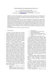
ABSTRACT
IGCC technology has demonstrated its feasibility but efficiency and reliability can be improved.
So that, an operation window is presented as a tool for optimising gasifier operation.
Two models of entrained flow gasifiers (one simple and the other more complex) are validated
with a large set of actual plant operation periods. The two models are used to build operation
windows, which are graphs where the main gasification parameters are related to the degrees of
freedom that the operator has. Comparison of the two windows allows to see limitations of the
simple model and to understand the gasifier operation.
A general method for building experimental operation windows only from plant data has been
developed. When the method is applied to the gasifier, tendencies of the windows are the same of
those of the model-made windows.
In conclusion, operation windows are practical tools that help to operate and diagnose a system
(e.g. a gasifier). They allow to understand how it works, to optimise its operation and to avoid
wrong operation that may cause plant shut off.
Keywords: Gasification, IGCC, Operation, Optimisation
NOMENCLATURE
C Carbon content in fuel
CGE Cold gas efficiency [%]
d Distance
daf Dry and ash free
i Real operation point
j Point in a iso-line
k Point in four-point group
LHV Low heating value [kJ/kg]
max Maximum
min Minimum
p Parameter
rel Relative
x Independent variable
y Independent variable
z Dependent variable
* Corresponding author: Phone: +34 976 76 25 82 Fax: +34 976 73 20 78 E-mail: suson@unizar.es
+ Thermoeconomic Diagnosis Group.
0 Coordenate of point in a iso-line
δ Increment
INTRODUCTION
Coal gasification is an efficient and
environmentally friendly way to use coal not only
to generate electricity in Integrated Gasification
Combined Cycle (IGCC) power plants, but also to
produce hydrogen and syngas for the chemical
industry [1-5]. However, right operation of a
gasifier is very complex for two reasons.
First, actual operating conditions usually differ
from design conditions because experience in
gasifiers operation is very small compared to
expertise on conventional equipment such as

oilers. Besides, design fuel is sometimes modified
by adding coke, biomass... So that, gasifier
working should be revised by using experience.
Second, proper gasifier operation is more critical
than boiler operation, because it does not consist in
just maximising efficiency but other issues, that in
turn requires keeping several output variables (gas
composition and gasification temperature) in
correct ranges and maximising fuel/gas conversion
by adjusting two input variables (oxygen and
steam that are introduced in the gasifier).
Gasification temperature is a variable that cannot
be measured but has to be kept in a right range
because it determines not only efficiency but also
safe operation. In oxygen-blown slagging gasifiers
an error in oxygen measurement could cause either
very high temperatures that can damage the
equipment or temperatures under slagging point
that can stop slag flow and blocking. Besides,
although output variables could be considered
separately, a modification in an input variable
implies changes in all output variables, so that all
dependencies should be understood and integrated.
In conclusion, to operate the gasifier it is necessary
to use criteria corresponding to the gasifier
working not only in tendencies but also in absolute
values.
Elcogas IGCC Power Plant in Puertollano (Spain)
is a demonstration project where several European
companies work together. CIRCE has collaborated
with Elcogas for several years in operation plant
optimisation and diagnosis. The main achievement
of CIRCE work is the development of the TDG
system [6,7]. TDG is an acronym of
Thermoeconomic Diagnosis, which consists in
comparing two plant real stable operation periods,
determining the causes why efficiency varies and
quantifying the influence of each cause in
efficiency deviation. This information allows to
optimise the plant by comparing the influence of
malfunctions in plant efficiency to the cost of
solving these malfunctions.
A gasifier is not isolated; not only gas production
have an influence on the gas cleaning section and
on the combined cycle but also the combined cycle
and the air separation unit influence the gasifier
operation. TDG takes these interactions into
account but the relationship between gasifier
operation and gasifier working should be deeply
investigated.
The aim of this work is to transform a hard subject
that comprise several related variables into
something that can be used and applied by
operators and that could be implemented in the
plant control system. Operators need a practical
tool which help them to adjust gasifier operation in
few minutes (perhaps seconds), taking into account
several variables at the same time; so that, a
graphic tool is proposed.
The concept of operation window is applied to a
two dimensional graph which axes corresponds to
the input variables (oxygen/fuel ratio in x and
steam/fuel ratio in y) where the main output
variables evolution (temperature, efficiency and
concentration of the main components of the gas)
is plotted by using constant value lines.
Maximum and minimum values of the output
variables determine the region or the window
where the gasifier should be operated. Since there
are two degrees of freedom, there are several ways
to modify the value of an output variable and the
choice of the best one depends of the other output
variables. So that, a graph which shows all
important variables is very useful to operate the
gasifier in a safe and efficient way.
In this paper, two models are validated with a large
set of plant data and used to build operation
windows. These windows can be very useful to
explore new operation zones. However, to analyse
and improve actual operation it is better to take
advantage of expertise by building operation
windows from plant data without a model and to
use model-built windows as reference to provide
theoretical support. Since, unfortunately, there
were no methodologies to build operation windows
from plant data, a new general method has been
developed and applied to the case of study.
As a result, windows built by using a large amount
of plant data and supported by theoretical models
are obtained. These windows are very useful not
only to improve future operation but also to
analyse past operation, which is also a type of
diagnosis because it allows comparing differences
in gas composition and gasification temperature
and efficiency of several operation strategies.
Results show that, depending on operation mode,
gasifier efficiency may vary 3 percent, which
means about 5 MWe.
CHOICE OF THE SUPPORTING GASIFIER
MODEL
The PRENFLO (Pressurized ENtrained FLOw)
gasifier is fed with fuel (a mixture of coal and
petroleum coke), oxygen, steam and nitrogen,
which react at a high temperature becoming a

combustible gas (synthesis gas). This kind of
gasifier achieves very high carbon conversion in a
short reaction time. When the gas leaves the
reaction chamber, it is quickly cooled by a flow of
cold gas in order to lock gas phase equilibrium and
solidify the ash carried by the gas (most of ash
leaves the gasifier as slag that flows to the bottom).
Then, the gas is further cooled to get the right
temperature to be cleaned. Sensible heat of the gas
is used to generate steam, which is exported to the
steam cycle.
Boiling
Water
1
Pirolisis and volatiles
combustion
T ~ 2000ºC
Raw Gas + Fly Ash
Slag
1750 ºC
25 bar
Figure 1: Reaction chamber
Since the amount of fuel is determined by the gas
demand of the turbine and nitrogen is mainly used
to carry the fuel, the only degrees of freedom that
the operator has to control gasification reactions
are the amounts of oxygen and steam. These flows
are controlled by the oxygen/fuel and steam/fuel
ratios.
Two models of the reaction chamber were
available. The first one (constant fuel conversion)
is proposed by Van der Burgt [8,9] and was used to
the fine-tuning of the control system during
commisioning. This model considers constant fuel
conversion ratio, so that it avoids gasification
process simulation and only takes into account
matter and energy balances and gas phase
equilibrium.
The second one (variable fuel conversion) was
proposed by Martínez [10] to be used as the offdesign
simulator of the gasifier in the TDG system.
It divides gasification process into several stages,
studies gas-particle interaction and simulates gas
phase equilibrium. So that, this complex model
takes into account fuel conversion variation due to
gasification conditions modifications.
To adjust the two models, information provided by
the TDG System is used [6,7]. This system
connects to the plant information system and
4
3
Burner
2
Methane formation
Gasification
Burners
N2
O2 + H2O Secondary
Fuel
O2 + H2O Primary
Flame detector
Formation and
combustion of part of
the char.
identifies stable working periods. For each period,
TDG stores and validates information and, by
using data reconciliation and closing energy and
matter balances, determines the thermodynamic
state of the plant.
The information of 2,874 real operation periods
(which means 4,812 hours) filtered and processed
by this system is used to tune the models: in the
model proposed by Van der Burgt the fuel
conversion ratio is adjusted and in the Martínez
model the values of this ratio are used to adjust the
particle residence time.
To validate the models, relative average
experimental discrepancy (taking into account this
historical data) is calculated for gasification
temperature, main gas composition and CGE (Cold
Gas Efficiency, or a ratio between chemical energy
of the gas and chemical energy of the fuel). Results
are shown in Table 1.
Constant fuel Variable fuel
conversion conversion
Temperature 2.1% 2.4%
CGE 0.26% 0.8%
CO 0.20% 0.56%
H2 0.62% 0.43%
CO2 1.6% 4.9%
H2O 1.9% 5.3%
H2S 7.7% 7.9%
COS 8.25% 8.5%
Table 1: Relative average errors of the two models.
As can be seen, errors of CGE and the most
abundant species (CO, H2) are very small.
However, relative errors increase for the less
concentrated species. One remarkable result is that
errors of the constant conversion ratio model in
CGE, CO2 and H2O are lower than errors of the
variable conversion ratio model. This is due to the
limitations of working with actual plant data.
These difficulties increase when a more complex
model is used. However, errors of both models are
low and differences will be seen in next section by
comparing simulations in a zone wider than usual
operation region.
MODEL-BUILT OPERATION WINDOWS
Once the models have been presented and
validated, they are used to build reference
operation windows. In Figure 2, an operation
window built from the constant conversion model

is shown. This window has been plotted by using
information from a real operation period and by
modifying oxygen and steam ratios. As can be
seen, when oxygen or steam increases, CO2
increases and CO decreases. When oxygen
increases or steam decreases, temperature increases
and H2 decreases. Finally, CGE decreases when
oxygen increases and decreases slightly if steam
increases.
Steam ratio (kg steam/kg fuel daf)
Operation window. Constant conversion model.
0,18
CGE = 74%
CGE = 75%
CGE = 76%
CGE = 77%
0,16
CGE = 78%
T = 1600 ºC
T = 1700 ºC
T = 1800 ºC
0,14
T = 1900 ºC
58% CO
60% CO
0,12
62% CO
64% CO
20% H2
21% H2
0,1
22% H2
23% H2
1% CO2
0,08
0,69 0,71 0,73 0,75
2% CO2
3% CO2
4%CO2
Oxygen ratio (Nm3 pure O2/kg fuel daf)
5% CO2
Figure 2: Constant conversion operation window.
In Figure 3, an equivalent operation window using
the variable conversion model is shown. In this
model, when temperature decreases, fuel
conversion decreases. As a result, CGE reaches a
maximum and, as long as oxygen decreases fuel
conversion decreases, CO and CO2 variations are
lower. As can be seen, when oxygen ratio is high
and conversion increases to 100 percent (right side
of the window) the constant conversion window
becomes similar to variable conversion window
but values are displaced. This displacement is due
to that fuel conversion in constant conversion
model has been adjusted to 98.5 percent.
Steam ratio (kg steam/kg fuel daf)
0,18
0,16
0,14
0,12
0,1
Operation window. Variable conversion model.
0,08
0,69 0,71 0,73 0,75
Oxygen ratio (Nm3 pure O2/kg fuel daf)
CGE = 75,5%
CGE = 76%
CGE = 76,5%
CGE = 77%
CGE = 77,5%
T = 1700 ºC
T = 1800 ºC
T = 1900 ºC
58% CO
60% CO
62% CO
20% H2
21% H2
22% H2
23% H2
2% CO2
3% CO2
4%CO2
5% CO2
Figure 3: Variable conversion operation window.
The windows built by using two models can help
to compare the models: although both can fit plant
data quite accurately, when the operation zone is
expanded they show differences. Besides, they are
an example of how operation windows can be very
useful to plot information in order to understand
the gasifier working and to optimise its operation.
The constant conversion model was very useful to
tune the control system in a small operation zone
but it does not provide good results when this zone
is expanded. To do so, a variable conversion model
should be used. However, it might be difficult to
tune this complex model with plant data
corresponding to a reduced operation zone, as
could be seen when both models were validated. In
conclusion, it is better to build plant operation
windows directly from plant data and to use the
models to give theoretical support to the plant
results. So that, a new method to build operation
windows from plant data is presented and applied.
METHODOLOGY FOR BUILDING
OPERATION WINDOWS FROM PLANT
DATA
A method to get a family of points that
corresponds to an iso-line (line of constant value of
a dependent variable) in a window (constant value
of a parameter) is explained. This process can be
repeated for the other iso-lines, for the other values
of the parameter and for the other dependent
variables until getting all the windows built.
A dependent variable z that depends on two
independent variables (x and y) and a parameter (p)
is considered:
z = z(
x,
y,
p)
(1)
In the example of the gasifier, x is the oxygen ratio,
y the steam ratio and p the load. The dependent
variable z can be temperature, CGE or one
concentration. Graphically, the iso-line is the
intersection of the surface p = p0 and the plane z =
z0 (Figure 4).
A group of operation points characterised by the
values of the four variables (x, y, p, z)i is available
(the 2,874 actual operation points used to tune the
models) and we want to transform it into another
group of points (x0, y0, p0, z0)j where p0 and z0 are
given by the window and the iso-line respectively,
and x0 and y0 are the unknown quantities. The
procedure for doing this transformation consists of
building groups of four points and, by considering
that the z function is linear in small zones,
obtaining one new point from each group.

X
Figure 4: Methodology scheme
The first step is to make four-point groups. To
select them, the following conditions are imposed:
i) Their p and z values should be near to p0 and z0:
p δ ≤ p ≤ p + δ k = 1..
(2)
0 − P k 0 P 4
z0 − δ z ≤ zk
≤ z0
+ δ z = 1..
4
k (3)
ii) Once a point 1 that accomplish the previous
conditions has been selected, the other three points
are chosen according to the following criteria:
p − p ⋅ p − p >
(4)
( 1 0 ) ( 2 0 ) 0
( 1 − z0
) ⋅ ( z2
− z0
) < 0
( 1 − p0
) ⋅ ( p3
− p0
) < 0
( 1 − z0
) ⋅ ( z3
− z0
) > 0
( 1 − p0
) ⋅ ( p4
− p0
) < 0
( − z ) ⋅ ( z − z ) < 0
z (5)
p (6)
z (7)
p (8)
z 1 0 4 0
(9)
iii) If for each point 1 (for each group) there are
various possible points 2, 3 or 4, the points that
minimise the following expression are chosen:
2
d k =
2 ( xk
− x1
)
2
x − x
+
2 ( yk
− y1
)
2
y − y
(10)
( ) ( ) +
max min
max min
( )
( ) 2
2
pk − p1
+ k = 2..
4
p − p
max
Z
P1
min
P = P0
Z = Z0
Where distances are divided into the maximum
distance in order to avoid scale effect. A maximum
dk is also imposed.
The first condition is only a filter to select the
points nearer to the iso-line. By using only this
condition an operation window could be built, but
if δ values were small the window would have very
few points and if δ values were high the window
P3
P0
P2
P4
ISO-LINE
Y
clarity would decrease. Hence, a more elaborated
method is proposed.
The second and third conditions are used to build
the four-point groups from the points that have
passed the first condition filter. The second
condition is proposed to ensure a good distribution
of the four points around the unknown point. Since
the surface p = p0 and the plane z = z0 determine
four regions in the space, each point of the group
should be in a different region. Due to the third
condition the four points are in a small region, in
which the z function can be considered as linear
(Figure 4).
Once the four-point groups have been built, the
pairs (x0, y0) are generated (one pair from each
group). To obtain these pairs, the dependent
variable is expressed in each one of the four points
with a first order Taylor series around the point (x0,
y0, p0).
zk = z0
+ z x ⋅ ( xk
− x0
) + z y ⋅ ( yk
− y0
)+ (11)
+ z p ⋅ ( pk
− p0
) k = 1..
4
As there are four equations and five unknown
quantities (zx, zy, zp, x0 and y0) an additional
condition should be added. This condition is that
the following expression (distance from the new
point to the old ones) should be minimum:
4
2
2
⎛ ( ) ( ) ⎞
2 x
∑ ⎜ k − x0
yk
− y0
d =
⎟
⎜
+
(12)
2
2
= ( ) ( ) ⎟
k 1 ⎝ xmax
− xmin
ymax
− ymin
⎠
By solving the system for each four-point group, a
family of points is obtained. These points, when
plotted, form the iso-line. Since this linear system
is solved for each four-point group, this
methodology can be used for any curve shape
although it is based on first order Taylor series.
GASIFIER OPERATION WINDOW FROM
PLANT DATA
The methodology described above has been
applied to build an operation window of the
gasifier for a 90% load (p=90). Plant data are the
same that were used to validate the models. Since
the iso-lines are now groups of points, it is more
convenient to use one graph for each dependent
variable. The graph that can be seen more clearly is
the concentration of CO2 (Figure 5).
Operation windows show the same tendency as
model-built windows but they are limited to a more
reduced zone. In this zone, both models give
similar values, which explain why errors are
reduced. The graphs of the other dependent

variables are not as clear as the graph of CO2 but,
except the graph of H2, the tendency can be
appreciated. All windows can be seen in [11].
Steam ratio (kg/kg fuel daf)
Steam ratio (kg/kg fuel daf)
Steam ratio (kg/kg fuel daf)
0,18
0,16
0,14
0,12
0,1
CO2
0,08
0,69 0,71 0,73 0,75
O2 ratio (Nm3 pure O2/kg fuel daf)
0,18
0,16
0,14
0,12
0,1
Figure 5: CO2 operation window
CO2
0,08
0,69 0,71 0,73 0,75
O2 ratio (Nm3 pure O2/kg fuel daf)
CO2 = 2,75%
CO2 = 3%
CO2 = 3,25%
CO2 = 3,5%
CO2 = 3,75%
CO2 = 4%
CO2 = 4,25%
CO2 = 2,75%
CO2 = 3%
CO2 = 3,25%
CO2 = 3,5%
CO2 = 3,75%
CO2 = 4%
CO2 = 4,25%
Figure 6: CO2 operation window, using ratio
transformation and average fuel composition
0,18
0,16
0,14
0,12
0,1
H2
0,08
0,69 0,71 0,73 0,75
O2 ratio (Nm3 pure O2/kg fuel daf)
H2 = 20,5%
H2 = 21%
H2 = 21,5%
H2 = 22%
H2 = 22,5%
H2 = 23%
Figure 7: H2 operation window, using ratio
transformation and average fuel composition
To improve the resolution of the graphs of
compositions, information about the fuel
composition should be included. One way to do
this is by applying the method to build the
windows not to the oxygen and steam ratios but to
a ratios O/C and H/O that are calculated by
dividing the total amount of carbon, hydrogen and
oxygen (taking into account the carbon, oxygen
and hydrogen contained in fuel, the steam and the
oxygen). Then, the pairs (x0, y0) should be
transformed from O/C and H/O to oxygen/fuel and
steam/fuel ratios by using an average fuel
composition. This idea is based on the fact that,
since the fuel conversion and final equilibrium
constants are roughly constant and the influence of
nitrogen and sulphur can be neglected, the final gas
composition only depends on the relations between
carbon, oxygen and hydrogen. As can be seen in
Figures 7 and 8, the graph of CO2 becomes clearer
and the graph of H2 shows a tendency (while the
steam and oxygen ratios were used directly no
tendency was seen). The improvement obtained in
the H2 is due to the small molecular mass of this
element, which made that a small change in the
fuel composition causes an important dispersion in
the gas composition.
Although the use of O/C and H/O ratios improves
the clarity of composition windows, this
transformation is not suitable for energy related
variables (temperature and CGE) because it mixes
all sources of carbon, oxygen and hydrogen
without taking into account the variation of LHV
that a modification of fuel composition implies.
One way to introduce fuel LHV and to use O/C
and H/O ratios in the CGE window is by
representing not CGE but a relative CGE [11].
This variable is calculated by introducing a
correction factor fCGE that allows to take into
account variations in the relation of fuel LHV and
carbon content in the fuel:
CGE = CGE ⋅ f (13)
f
CGE
rel
CGE
38,
500
= (14)
⎛ LHV fuel ⎞
⎜ ⎟
⎜ C ⎟
⎝ fuel ⎠
( kJ / kg )
For the analysed periods, this factor varies from
0.982 to 1.015. In figure 6 an operation window of
CGErel built by using O/C and H/O ratios is shown.
The iso-lines show that the gasifier is operated in
the high fuel conversion zone, by using oxygen
ratios above the maximum CGE point.

Figure 8: Relative CGE operation window, using
ratio transformation and average fuel composition
Plant data operation windows presented in this
section shows the same tendencies as model-built
operation windows but the iso-lines are slightly
displaced. For example, the maximum CGE point
would be displaced towards the left side of the
plant data operation windows, while in the
variable-conversion model operation window this
point is near the centre. This aspect demonstrates
that it has been very useful to build these windows
from plant data.
However, if these windows are going to be used by
plant operators, point families should be
transformed into lines and all variables should be
plotted in the same graph (Figure 9).
Steam ratio (kg/kg fuel daf)
Steam ratio (kg/kg fuel daf)
0,18
0,16
0,14
0,12
0,1
0,18
0,16
0,14
0,12
0,1
Figure 9: Operation window for operators use
CONCLUSIONS
CGE rel
0,08
0,69 0,71 0,73 0,75
O2 ratio (Nm3 pure O2/kg fuel daf)
Operation window 90% load.
0,08
0,69 0,71 0,73 0,75
O2 ratio (Nm3 pure O2/kg fuel daf)
CGE = 75%
CGE = 75,5%
CGE = 76%
CGE = 76,5%
CGE = 77%
CGE = 77,5%
CGE = 78%
CGE = 73%
CGE = 74%
CGE = 75%
CGE = 76%
T = 1700 ºC
T = 1750 ºC
T = 1800 ºC
T = 1850 ºC
T = 1900 ºC
CO = 59%
CO = 60%
CO = 61%
CO = 62%
CO = 63%
H2 = 21 %
H2 = 21,5 %
H2 = 22 %
H2 = 22,5 %
H2 = 23 %
H2 = 23,5 %
CO2 = 2%
CO2 = 2,5%
CO2 = 3%
CO2 = 3,5%
Since the gasifier runs with a high and constant
fuel conversion ratio and variations of this
parameters can not be detected, a simple model
like the one proposed by Van der Burgt is enough
to reconcile plant data. However, if a wider
operation range is explored, a more sophisticated
model with variable fuel conversion ratio is
needed.
An operation window is a practical tool, which can
help to understand how the gasifier works and to
operate it in an efficient way. By comparing the
two model-built windows, constant conversion
model limitation can be seen.
Although the models are useful to tune control
system and to analyse new operation zones, to
study actual gasifier operation it is better to build
windows from plant data. Hence a new method is
proposed. It is a general methodology that has
three advantages: 1) it allows to introduce more
than one independent variable, 2) it does not
impose any type of graph (linear, polynomial) and
3) it can be applied to real operation periods
because it does not need even distributed data.
Thus, it can be very useful for studying any
system.
Operation windows shown in this paper are
currently being used in Puertollano power plant
daily operation. Thanks to this work, operators
have a graph in which the consequences of their
actions are clearly plotted, which can avoid errors
and plant failures. Since plant data windows shows
that in usual operation CGE can vary about 3
points, which means about 5 MW, the use of the
windows can improve plant efficiency
significantly.
SUMMARY OF THE METHODOLOGY
If coal is going to play an important role as
abundant and even distributed energy source in the
XXI century, clean and efficient technologies
should be used. Perhaps, the most promising
technique is gasification, because it allows going
into the hydrogen society and also facilitates the
CO2 capture and disposal of. But gasification is not
combustion. The optimum working condition of a
gasifier is only obtained through the control of the
reactive agents taking place in the reaction
chamber (concentration, pressure and temperature),
in opposition to combustion, which is a reaction
totally developed.
Accordingly, the problem of obtaining operation
windows is an universal problem that every
existing or planned gasification plant will have to
face to. This problem cannot be solved by using
only a pure theoretical analysis but an empirical
feedback helping to solve the fine-tuning of a
gasifier is also needed. As already said, this could
suppose a lost in gasifier efficiency of as much as 3

percent. Therefore, the methodology developed in
this paper can be of use for new IGCC plants
provided that the experience gained from an
already existing plant is considered.
So, the methodology presented in this paper can be
summarised as follows:
i) Previously, it should be necessary to have
an on-line system that provides information
about gasifier efficiency, pressures,
temperatures and so on, which is nowadays a
common tool technique.
ii) A theoretical analysis should be carried out
by using a model in order to obtain tendencies.
The model should have been tuned by using
plant data. Steam and oxygen ratios should be
considered as independent variables and
temperature, main gas components and
efficiency as dependent variables. An
operation window should be used to plot all
dependencies in one graph.
iii) Operation windows from plant data should
be built by using the method proposed in this
paper. If these windows did not show the same
tendencies as the model-built ones, hypothesis
assumed in the model should be revised.
iv) Finally, conclusions about how to modify
operation to increase efficiency should be
obtained and a clearer version of the windows
(substituting the points to lines) should be
provided to operators.
ACKNOWLEDGMENTS
The authors would like to acknowledge the
management of Elcogas power plant for their
faithful collaboration at every moment, specially to
Ing. Francisco García-Peña, Engineering &
Maintenance manager, Ing. Alejandro Muñoz,
head of technology, Ing. Silvia Burgos, head of the
R&D group, Ing. Francisco Puente and Ing. Pedro
Casero, for their constant and active support to this
idea.
REFERENCES
[1] Pisa J. Análisis Termoeconómico aplicado al
diseño de plantas IGCC. PhD Thesis.
Department of Mechanical Engineering,
University of Zaragoza. 1996.
[2] Stiegel GJ, Maxwell RC. Gasification
technologies: the path to a clean, affordable
energy in the 21 st century. Fuel Processing
Technology 2001;71:1-3:79-97.
[3] European Commission, Directorate-General
for Energy (DGXVII). Clean coal
technologies handbook. Section 7:
Gasification.
[4] European Commission, Directorate-General
for Energy (DGXVII). Clean coal
technologies handbook. Section8: Integrated
Gasification Combined Cycle.
[5] Hoffman EJ. Coal Gasifiers. Energon, 1981.
[6] García-Peña F, Gálvez A, Correas L, Casero
P. Advanced operation diagnosis for power
plants. Performance monitoring and cost
assessment in Puertollano IGCC. PowerGen
Europe 2000, Helsinki, 2000.
[7] García-Peña F, Correas L, Millán JL.
Improving O&M at IGCC Puertollano
through termo-economic diagnosis.
PowerGen Europe 2001, Brussels, 2001.
[8] Van der Burgt MJ. Techno-historical aspects
of coal gasification in relation to IGCC
plants. Private communication. 1998.
[9] Ayerbe E. Elaboración, estudio y validación
de ventanas de operación de un gasificador de
tipo lecho arrastrado siguiendo el modelo
propuesto por Maarten J. Van der Burgt. MSc
Thesis. Department of Mechanical
Engineering, University of Zaragoza. 2002.
[10] Usón S, Martínez A, Valero A, Correas L.
Application of a gasifier model to the
theoretical study of co-gasification of coal
and biomass at an IGCC power plant. In:
Procceedings of the 16 th International
Conference on Efficiency, Costs,
Optimisation, Simulation and Environmental
Impact of Energy Systems, Copenhagen,
2003.
[11] Usón S. Aplicación de un modelo cinéticoquímico
al estudio del gasificador de una
central GICC. Validación y estudio teórico de
la cogasificación con biomasa. MSc Thesis.
Department of Mechanical Engineering,
University of Zaragoza.2002.