Experiments with Supersonic Beams as a Source of Cold Atoms
Experiments with Supersonic Beams as a Source of Cold Atoms
Experiments with Supersonic Beams as a Source of Cold Atoms

You also want an ePaper? Increase the reach of your titles
YUMPU automatically turns print PDFs into web optimized ePapers that Google loves.
Copyright<br />
by<br />
Adam Alexander Libson<br />
2012
The Dissertation Committee for Adam Alexander Libson<br />
certifies that this is the approved version <strong>of</strong> the following dissertation:<br />
General Methods <strong>of</strong> Controlling Atomic Motion:<br />
<strong>Experiments</strong> <strong>with</strong> <strong>Supersonic</strong> <strong>Beams</strong> <strong>as</strong> a <strong>Source</strong> <strong>of</strong> <strong>Cold</strong><br />
<strong>Atoms</strong><br />
Committee:<br />
Mark G. Raizen, Supervisor<br />
Michael F. Becker<br />
Herbert L. Berk<br />
John W. Keto<br />
Greg O. Sitz
General Methods <strong>of</strong> Controlling Atomic Motion:<br />
<strong>Experiments</strong> <strong>with</strong> <strong>Supersonic</strong> <strong>Beams</strong> <strong>as</strong> a <strong>Source</strong> <strong>of</strong> <strong>Cold</strong><br />
<strong>Atoms</strong><br />
by<br />
Adam Alexander Libson, B.A.<br />
DISSERTATION<br />
Presented to the Faculty <strong>of</strong> the Graduate School <strong>of</strong><br />
The University <strong>of</strong> Tex<strong>as</strong> at Austin<br />
in Partial Fulfillment<br />
<strong>of</strong> the Requirements<br />
for the Degree <strong>of</strong><br />
DOCTOR OF PHILOSOPHY<br />
THE UNIVERSITY OF TEXAS AT AUSTIN<br />
December 2012
For Kirsten
Acknowledgments<br />
First and foremost, I would like to thank my advisor, Mark Raizen. It h<strong>as</strong><br />
been a privilege to work <strong>with</strong> Mark for my graduate career, and I am continually<br />
amazed by his creative approach to physics research. I have also been thankful for the<br />
supportive environment he h<strong>as</strong> fostered in the lab, which makes the daily frustrations<br />
<strong>of</strong> experimental work much e<strong>as</strong>ier to bare.<br />
I would also like to thank my wife, Kirsten. Having a fellow physicist at home,<br />
and my partner at work, led to additional stress, but the space provided by our work<br />
on different experiments made all the difference. My ability to discuss physics “after<br />
hours” <strong>with</strong> her provided me <strong>with</strong> the solutions to many problems, and her emotional<br />
support in the lab got me through quite a few crises.<br />
Much <strong>of</strong> my time in the lab w<strong>as</strong> spent <strong>with</strong> my co-workers on the beam slowing<br />
experiment, which h<strong>as</strong> truly been a team effort. Tom Mazur is a gifted experimental-<br />
ist, and h<strong>as</strong> been a fant<strong>as</strong>tic person to work <strong>with</strong>. Very few people hold themselves<br />
to <strong>as</strong> high a standard <strong>as</strong> Tom does, and this certainly shows in his work and in his<br />
approach to physics. Isaac Chavez started working in the lab at the same time I<br />
did, and his mechanical aptitude and no fear approach helped us in the lab on many<br />
occ<strong>as</strong>ions. Travis Bannerman joined the experiment after working <strong>with</strong> single photon<br />
cooling and l<strong>as</strong>er cooling in general on the rubidium experiment, and this experience<br />
w<strong>as</strong> essential in setting up the hydrogen l<strong>as</strong>er, since he w<strong>as</strong> <strong>with</strong>out doubt our l<strong>as</strong>er<br />
guru.<br />
I also had the ple<strong>as</strong>ure to work <strong>with</strong> two fant<strong>as</strong>tic post-docs, Ed Narevicius<br />
and Rob Clark. Ed w<strong>as</strong> a fant<strong>as</strong>tic person to work <strong>with</strong>, and his guidance certainly<br />
v
provided me <strong>with</strong> plenty <strong>of</strong> insight. Ed, additionally, makes a mean grilled rack <strong>of</strong><br />
lamb, and I greatly enjoyed spending time <strong>with</strong> him, his wife Julia, and their son,<br />
Yoav. Rob worked <strong>with</strong> me on the hydrogen experiment, and his l<strong>as</strong>er experience<br />
l<strong>as</strong>er helped us to get UV light. I also had many fun evenings at Clark Tavern.<br />
I also wish to thank each <strong>of</strong> the Wurzberg students I worked <strong>with</strong> during my<br />
time here. Max Riedel and Christoph Schaeff worked <strong>with</strong> me on the rotor experiment.<br />
Max worked <strong>with</strong> me getting the rotor <strong>of</strong>f the ground, and I would like to thank him<br />
for his contributions there. More important to me though is the friendship he provided<br />
during my first year. Whether playing badminton, listening to music, or just eating<br />
ice cream, Max w<strong>as</strong> a great guy to hang out <strong>with</strong>. Christoph worked to get the LiF<br />
<strong>as</strong>pect <strong>of</strong> the rotor working, and his devotion to the experiment and to the Austrian<br />
body building method both impressed me. Finally, I must thank Christian Parthey.<br />
Christian worked <strong>with</strong> me on the magnetic slowing <strong>of</strong> neon, and w<strong>as</strong> a fant<strong>as</strong>tic person<br />
to work <strong>with</strong> in the lab. He is also a great friend and someone I spent a lot <strong>of</strong> my<br />
non-lab time <strong>with</strong> while he w<strong>as</strong> here. I would also like to point out that his skill set<br />
is not limited to the lab <strong>as</strong> I’ve observed some impressive moves on the rock.<br />
As I am leaving, the hydrogen experiment will be run by Maria Becker and<br />
Tom. Maria started at the beginning <strong>of</strong> this year and h<strong>as</strong> quickly become an essential<br />
part <strong>of</strong> the team, <strong>as</strong> well <strong>as</strong> an arduino interlock expert. I have no doubts that the<br />
experiment is in good hands.<br />
Besides the people I worked <strong>with</strong> directly, there are many other Raizen lab<br />
members who provided me <strong>with</strong> good times and good physics when I needed them.<br />
Uzi Even worked <strong>with</strong> us on the supersonic beam side and greatly shorted my learning<br />
curve regarding beam physics. Gabe w<strong>as</strong> a great source <strong>of</strong> knowledge regarding single<br />
photon cooling and he also w<strong>as</strong> the driving force behind the first and only Raizen<br />
lab Salt Lick Contest. David is a fant<strong>as</strong>tic physicist, <strong>with</strong> a meticulous approach<br />
vi
to problems, and I frequently went to him if there w<strong>as</strong> a concept that confused<br />
me. Hrishi, Tongcang, and Kevin were all wonderful people to work <strong>with</strong>. Simon<br />
and Akarsh are sure to do great things <strong>with</strong> their bead experiment, and Jamie and<br />
Roderigo are quickly getting the focusing experiment going. Jianyong is rapidly<br />
learning the lithium experiment, and he is sure to do great things <strong>with</strong> it in the future.<br />
Melissa w<strong>as</strong> our lab’s high energy person, and I had many wonderful discussions <strong>with</strong><br />
her while sharing an <strong>of</strong>fice. I am sure she will find success in her new role leading the<br />
company that h<strong>as</strong> grown out <strong>of</strong> her research here. I thank all <strong>of</strong> you for your help<br />
and friendship.<br />
I have received considerable support from other members <strong>of</strong> the UT physics<br />
community <strong>as</strong> well, and I would particularly like to thank the machine and cryoshop<br />
here. It is thanks to the skills <strong>of</strong> the machinists that some <strong>of</strong> our more complicated<br />
designs came together and worked <strong>as</strong> intended, and the shop w<strong>as</strong> certainly there<br />
for me to fix things that had gone wrong. I would particularly like to thank Allan<br />
for discussing my designs <strong>with</strong> me and going over the best way to approach a part.<br />
Also deserving <strong>of</strong> special mention are Lanny and Ed, who provided me <strong>with</strong> excellent<br />
support from the cryo and vacuum shop. Finally, I would like to thank Jack, who<br />
taught me everything I know about machining. When we needed a part RIGHT<br />
NOW, Jack w<strong>as</strong> there to help me figure out how to make it. My heartfelt thanks to<br />
everyone on the third floor. I would also like to thank Elena, Mary Beth, and Olga on<br />
the 14th floor. Their tireless efforts make the lab run much smoother and facilitate<br />
much <strong>of</strong> what we do downstairs.<br />
In addition to my fellow lab members, I would like to thank my parents for<br />
providing me <strong>with</strong> the support and love to get where I am now. Visits home frequently<br />
provided a much needed break, and life here w<strong>as</strong> certainly less stressful knowing that<br />
they were there to support me. I would also like to thank my new family for all <strong>of</strong><br />
vii
their support and for welcoming me into their lives.<br />
Finally, I would like to acknowledge the University <strong>of</strong> Tex<strong>as</strong> at Austin for their<br />
support in the form <strong>of</strong> the William S. Livingston Graduate Fellowship.<br />
viii<br />
Adam Libson
General Methods <strong>of</strong> Controlling Atomic Motion:<br />
<strong>Experiments</strong> <strong>with</strong> <strong>Supersonic</strong> <strong>Beams</strong> <strong>as</strong> a <strong>Source</strong> <strong>of</strong> <strong>Cold</strong><br />
<strong>Atoms</strong><br />
Adam Alexander Libson, Ph.D.<br />
The University <strong>of</strong> Tex<strong>as</strong> at Austin, 2012<br />
Supervisor: Mark G. Raizen<br />
This dissertation discusses several recently developed experimental techniques<br />
for controlling the motion <strong>of</strong> neutral atoms. While l<strong>as</strong>er cooling and evaporative<br />
cooling have been extremely successful and have been in widespread use for many<br />
years, these techniques are only applicable to a few atomic species. <strong>Supersonic</strong> beams<br />
provide a general method <strong>of</strong> producing cold atoms in the co-moving frame, but their<br />
speeds are typically several hundreds <strong>of</strong> meters per second in the lab frame. Methods<br />
to slow and control atoms cooled by supersonic expansion are detailed.<br />
A method for controlling the velocity <strong>of</strong> a cold beam <strong>of</strong> ground state helium<br />
using specular reflection from single crystal surfaces is demonstrated. The velocity <strong>of</strong><br />
the beam is shown to be continuously tunable, and beam velocities <strong>as</strong> slow <strong>as</strong> 265m/s<br />
are created from an initial beam speed <strong>of</strong> 511 m/s.<br />
Magnetism is a nearly universal atomic phenomenon, making magnetic control<br />
<strong>of</strong> atomic motion a very general technique. Magnetic stopping <strong>of</strong> supersonic beams<br />
<strong>of</strong> met<strong>as</strong>table neon and molecular oxygen is demonstrated using a series <strong>of</strong> pulsed<br />
electromagnetic coils. Neon is slowed from 446 m/s to 56 m/s, and oxygen is slowed<br />
from 389 m/s to 83 m/s, removing over 95% <strong>of</strong> the kinetic energy. The experimental<br />
technique is described in detail, and the theory and principle are discussed. An<br />
ix
experiment for slowing and trapping <strong>of</strong> atomic hydrogen isotopes at around 100 mK<br />
using a room temperature apparatus is described. A method for further cooling <strong>of</strong><br />
magnetically trapped hydrogen ensembles, single-photon cooling, is proposed.<br />
x
Table <strong>of</strong> Contents<br />
Acknowledgments v<br />
Abstract ix<br />
List <strong>of</strong> Tables xiv<br />
List <strong>of</strong> Figures xv<br />
Chapter 1. Introduction 1<br />
1.1 Cooling an Effusive Beam . . . . . . . . . . . . . . . . . . . . . . . . 2<br />
1.1.1 L<strong>as</strong>er Cooling . . . . . . . . . . . . . . . . . . . . . . . . . . . . 2<br />
1.1.2 Buffer-G<strong>as</strong> Cooling . . . . . . . . . . . . . . . . . . . . . . . . . 3<br />
1.2 Methods <strong>of</strong> Controlling <strong>Supersonic</strong> <strong>Beams</strong> . . . . . . . . . . . . . . . . 4<br />
1.3 Dissertation Outline . . . . . . . . . . . . . . . . . . . . . . . . . . . . 5<br />
Chapter 2. An Overview <strong>of</strong> <strong>Supersonic</strong> <strong>Beams</strong> 7<br />
2.1 Thermodynamics <strong>of</strong> Ideal G<strong>as</strong>es . . . . . . . . . . . . . . . . . . . . . 8<br />
2.1.1 Steady State G<strong>as</strong> Flow in 1D . . . . . . . . . . . . . . . . . . . 9<br />
2.1.2 Mach Number and <strong>Supersonic</strong> <strong>Beams</strong> . . . . . . . . . . . . . . 11<br />
2.1.3 <strong>Supersonic</strong> Beam Velocities . . . . . . . . . . . . . . . . . . . . 12<br />
2.2 The <strong>Supersonic</strong> Beam <strong>as</strong> a Bright General <strong>Source</strong> <strong>of</strong> <strong>Cold</strong> <strong>Atoms</strong> and<br />
Molecules . . . . . . . . . . . . . . . . . . . . . . . . . . . . . . . . . 13<br />
2.3 The Even-Lavie Nozzle for Generating Pulsed <strong>Beams</strong> . . . . . . . . . 16<br />
Chapter 3. Slowing <strong>Supersonic</strong> <strong>Beams</strong> via Specular Reflection: The<br />
Atomic Paddle 20<br />
3.1 Using Helium for Atom Optics <strong>Experiments</strong> . . . . . . . . . . . . . . 22<br />
3.2 Reflecting <strong>Atoms</strong> from Surfaces: Atomic Mirrors . . . . . . . . . . . . 23<br />
3.2.1 Crystal Choice: Si(111) . . . . . . . . . . . . . . . . . . . . . . 25<br />
3.2.2 Crystal Preparation and Wet Etching . . . . . . . . . . . . . . 26<br />
3.2.3 Crystal Characterization . . . . . . . . . . . . . . . . . . . . . . 28<br />
3.3 The Experimental Apparatus . . . . . . . . . . . . . . . . . . . . . . . 28<br />
3.3.1 The Vacuum System . . . . . . . . . . . . . . . . . . . . . . . . 30<br />
3.3.2 The Rotor . . . . . . . . . . . . . . . . . . . . . . . . . . . . . 34<br />
xi
3.3.2.1 Initial Design . . . . . . . . . . . . . . . . . . . . . . . 34<br />
3.3.2.2 Vibration and Balancing . . . . . . . . . . . . . . . . . 39<br />
3.3.2.3 Improved Spindle Design . . . . . . . . . . . . . . . . . 42<br />
3.3.3 Detection . . . . . . . . . . . . . . . . . . . . . . . . . . . . . . 44<br />
3.3.4 Control Systems . . . . . . . . . . . . . . . . . . . . . . . . . . 44<br />
3.4 Data and Results . . . . . . . . . . . . . . . . . . . . . . . . . . . . . 46<br />
3.4.1 Static Reflection . . . . . . . . . . . . . . . . . . . . . . . . . . 47<br />
3.4.2 Beam Slowing . . . . . . . . . . . . . . . . . . . . . . . . . . . 48<br />
3.4.3 Crystal Lifetime . . . . . . . . . . . . . . . . . . . . . . . . . . 52<br />
3.5 Potential Applications . . . . . . . . . . . . . . . . . . . . . . . . . . 54<br />
Chapter 4. The Atomic and Molecular Coilgun: Using Pulsed Magnetic<br />
Fields to Slow <strong>Supersonic</strong> <strong>Beams</strong> 56<br />
4.1 <strong>Atoms</strong> in External Magnetic Fields . . . . . . . . . . . . . . . . . . . 57<br />
4.1.1 The Zeeman Effect . . . . . . . . . . . . . . . . . . . . . . . . . 58<br />
4.1.2 The P<strong>as</strong>chen-Back Effect . . . . . . . . . . . . . . . . . . . . . 61<br />
4.1.3 Adiabatic Following and Spin Flips . . . . . . . . . . . . . . . . 62<br />
4.2 Magnetic Fields from Electromagnetic Coils . . . . . . . . . . . . . . 63<br />
4.2.1 Switching <strong>of</strong> Electromagnetic Coils . . . . . . . . . . . . . . . . 65<br />
4.3 Principle <strong>of</strong> Operation . . . . . . . . . . . . . . . . . . . . . . . . . . 66<br />
4.3.1 Ph<strong>as</strong>e Stability . . . . . . . . . . . . . . . . . . . . . . . . . . . 69<br />
4.3.2 Electromagnetic Coils <strong>as</strong> a Waveguide . . . . . . . . . . . . . . 72<br />
4.4 Pro<strong>of</strong>-<strong>of</strong>-Principle Experiment: Slowing Met<strong>as</strong>table Neon . . . . . . . 74<br />
4.4.1 Beam Creation . . . . . . . . . . . . . . . . . . . . . . . . . . . 75<br />
4.4.2 18 Stage Coil Design . . . . . . . . . . . . . . . . . . . . . . . . 77<br />
4.4.3 18 Stage Electronics and Coil Switching . . . . . . . . . . . . . 78<br />
4.4.4 18 Stage Apparatus and Vacuum Chamber . . . . . . . . . . . 83<br />
4.4.5 18 Stage Data and Results . . . . . . . . . . . . . . . . . . . . 87<br />
4.5 The Atomic Coilgun: Stopping Met<strong>as</strong>table Neon . . . . . . . . . . . . 89<br />
4.5.1 64 Stage Coil Design . . . . . . . . . . . . . . . . . . . . . . . . 90<br />
4.5.2 64 Stage Electronics and Coil Switching . . . . . . . . . . . . . 94<br />
4.5.3 64 Stage Apparatus and Vacuum Chamber . . . . . . . . . . . 100<br />
4.5.4 64 Stage Data and Results . . . . . . . . . . . . . . . . . . . . 105<br />
4.6 The Molecular Coilgun: Stopping Molecular Oxygen . . . . . . . . . . 109<br />
4.6.1 Oxygen’s Magnetic Levels . . . . . . . . . . . . . . . . . . . . . 110<br />
4.6.2 Oxygen Beam Creation and Detection . . . . . . . . . . . . . . 111<br />
4.6.3 Oxygen Data and Results . . . . . . . . . . . . . . . . . . . . . 113<br />
xii
Chapter 5. Towards Trapping and Cooling <strong>of</strong> Atomic Hydrogen Isotopes<br />
116<br />
5.1 Hydrogen Motivation and Structure . . . . . . . . . . . . . . . . . . . 117<br />
5.2 The Hydrogen Apparatus . . . . . . . . . . . . . . . . . . . . . . . . . 119<br />
5.2.1 Slowing Coils and Electronics . . . . . . . . . . . . . . . . . . . 119<br />
5.2.1.1 Slowing Coil Geometry . . . . . . . . . . . . . . . . . . 120<br />
5.2.1.2 Slowing Coil Electronics and Switching . . . . . . . . . 121<br />
5.2.2 Trapping Coils and Electronics . . . . . . . . . . . . . . . . . . 125<br />
5.2.2.1 Principle <strong>of</strong> Operation <strong>of</strong> the Trap . . . . . . . . . . . 126<br />
5.2.2.2 Trapping Coil Geometry and Fields . . . . . . . . . . . 128<br />
5.2.2.3 Trapping Electronics and Switching . . . . . . . . . . . 130<br />
5.2.3 Beam Creation and Detection . . . . . . . . . . . . . . . . . . . 135<br />
5.2.4 Vacuum Chambers . . . . . . . . . . . . . . . . . . . . . . . . . 137<br />
5.3 Simulations <strong>of</strong> Hydrogen Trapping . . . . . . . . . . . . . . . . . . . . 141<br />
5.3.1 Slowing and Trapping . . . . . . . . . . . . . . . . . . . . . . . 142<br />
5.3.2 Ejection Simulations . . . . . . . . . . . . . . . . . . . . . . . . 145<br />
5.4 Future Directions . . . . . . . . . . . . . . . . . . . . . . . . . . . . . 147<br />
5.4.1 L<strong>as</strong>er Detection and Spectroscopy <strong>of</strong> Hydrogen Isotopes . . . . 148<br />
5.4.1.1 Two-Photon Excitation <strong>of</strong> Hydrogen . . . . . . . . . . 148<br />
5.4.1.2 The Hydrogen L<strong>as</strong>er . . . . . . . . . . . . . . . . . . . 152<br />
5.4.1.3 Spectroscopic Goals . . . . . . . . . . . . . . . . . . . . 155<br />
5.4.2 An Adiabatic Coilgun . . . . . . . . . . . . . . . . . . . . . . . 156<br />
5.4.3 Single-Photon Cooling <strong>of</strong> Hydrogen . . . . . . . . . . . . . . . . 157<br />
Appendix 164<br />
Appendix A. Reflection From a Spinning Rotor 165<br />
Bibliography 168<br />
Vita 189<br />
xiii
List <strong>of</strong> Tables<br />
4.1 Peak Magnetic Fields Me<strong>as</strong>ured for Different Lengths <strong>of</strong> TGG Crystal 100<br />
4.2 Neon Slowing Data Summary . . . . . . . . . . . . . . . . . . . . . . 106<br />
4.3 Oxygen Slowing Data Summary . . . . . . . . . . . . . . . . . . . . . 114<br />
xiv
List <strong>of</strong> Figures<br />
2.1 Comparison <strong>of</strong> effusive and supersonic velocity distributions . . . . . 14<br />
2.2 Section view <strong>of</strong> the Even-Lavie supersonic nozzle . . . . . . . . . . . . 17<br />
3.1 Calculated helium el<strong>as</strong>tic scattering fraction from Si(111) . . . . . . . 24<br />
3.2 AFM image <strong>of</strong> a p<strong>as</strong>sivated Si(111) crystal . . . . . . . . . . . . . . . 29<br />
3.3 CAD image <strong>of</strong> nozzle chamber . . . . . . . . . . . . . . . . . . . . . . 30<br />
3.4 CAD image <strong>of</strong> rotor chamber . . . . . . . . . . . . . . . . . . . . . . 31<br />
3.5 CAD image <strong>of</strong> the detection chamber . . . . . . . . . . . . . . . . . . 32<br />
3.6 CAD image <strong>of</strong> entire apparatus . . . . . . . . . . . . . . . . . . . . . 33<br />
3.7 CAD image <strong>of</strong> the rotor . . . . . . . . . . . . . . . . . . . . . . . . . 36<br />
3.8 Finite element calculation <strong>of</strong> the forces on a spinning rotor . . . . . . 36<br />
3.9 CAD image <strong>of</strong> the rotor <strong>with</strong> spindle, feedthrough, and motor . . . . 37<br />
3.10 CAD image <strong>of</strong> the large crystal holder . . . . . . . . . . . . . . . . . 38<br />
3.11 Me<strong>as</strong>urements <strong>of</strong> rotor vibration at different rotational speeds . . . . 40<br />
3.12 Finite element calculation <strong>of</strong> rotor vibrational modes . . . . . . . . . 41<br />
3.13 CAD image <strong>of</strong> the redesigned spindle . . . . . . . . . . . . . . . . . . 43<br />
3.14 Rotor triggering and reflection positions . . . . . . . . . . . . . . . . 45<br />
3.15 Time-<strong>of</strong>-flight pr<strong>of</strong>iles for direct and reflected beams . . . . . . . . . . 47<br />
3.16 Time-<strong>of</strong>-flight pr<strong>of</strong>iles for different rotor speeds . . . . . . . . . . . . . 49<br />
3.17 Plot <strong>of</strong> slowed beam velocity vs. crystal velocity . . . . . . . . . . . . 51<br />
3.18 Plot <strong>of</strong> reflected intensity vs time . . . . . . . . . . . . . . . . . . . . 53<br />
4.1 Angular momentum coupling in low field . . . . . . . . . . . . . . . . 59<br />
4.2 Example Zeeman shift for a 3 P2 state . . . . . . . . . . . . . . . . . . 60<br />
4.3 Angular momentum coupling in high field . . . . . . . . . . . . . . . 61<br />
4.4 Magnetic Field from a Single Loop Coil . . . . . . . . . . . . . . . . . 64<br />
4.5 Principle <strong>of</strong> operation <strong>of</strong> the coilgun . . . . . . . . . . . . . . . . . . . 68<br />
4.6 Ph<strong>as</strong>e Stability From Coil Timing . . . . . . . . . . . . . . . . . . . . 71<br />
4.7 Magnetic Field Magnitudes <strong>as</strong> a Function <strong>of</strong> Radial Position . . . . . 73<br />
4.8 Images <strong>of</strong> the Discharge Apparatus and Discharge . . . . . . . . . . . 76<br />
4.9 CAD Overview <strong>of</strong> Pro<strong>of</strong>-<strong>of</strong>-Principle Experiment Coils . . . . . . . . 78<br />
4.10 Finite Element Calculation <strong>of</strong> Magnetic Field in the 18 Stage Slowing<br />
Coils . . . . . . . . . . . . . . . . . . . . . . . . . . . . . . . . . . . . 79<br />
xv
4.11 Schematic <strong>of</strong> the 18 Stage Coil Driver Circuit . . . . . . . . . . . . . 80<br />
4.12 Current in 18 Stage Slowing Coil . . . . . . . . . . . . . . . . . . . . 82<br />
4.13 Temporal Pr<strong>of</strong>ile <strong>of</strong> the Magnetic Field in the 18 Stage Coil . . . . . 83<br />
4.14 CAD Image and Photo <strong>of</strong> 18 Stage Coilgun . . . . . . . . . . . . . . . 84<br />
4.15 CAD Image <strong>of</strong> the 18 Stage Coilgun in the Rotor Chamber . . . . . . 85<br />
4.16 Schematic <strong>of</strong> the MCP Bi<strong>as</strong> Circuit . . . . . . . . . . . . . . . . . . . 86<br />
4.17 Photos <strong>of</strong> the 18 Stage Coilgun and Chamber . . . . . . . . . . . . . 86<br />
4.18 Results <strong>of</strong> Ph<strong>as</strong>e Variation in 18 Stage Coilgun . . . . . . . . . . . . . 87<br />
4.19 Results <strong>of</strong> Current Variation in 18 Stage Coilgun . . . . . . . . . . . . 88<br />
4.20 Exploded CAD View <strong>of</strong> 64 Stage Coilgun Coil . . . . . . . . . . . . . 90<br />
4.21 64 Stage Slower Coil Assembly Process . . . . . . . . . . . . . . . . . 92<br />
4.22 Finite Element Calculation <strong>of</strong> the 64 Stage Coilgun Magnetic Field . 93<br />
4.23 Schematic <strong>of</strong> the 64 Stage Coil Driver Circuit . . . . . . . . . . . . . 94<br />
4.24 Photographs <strong>of</strong> the 64 Stage Coil Driver Board . . . . . . . . . . . . . 95<br />
4.25 Schematic <strong>of</strong> Faraday Rotation Setup . . . . . . . . . . . . . . . . . . 98<br />
4.26 Temporal Pr<strong>of</strong>ile <strong>of</strong> the Faraday Rotation in a 64 Stage Coilgun Coil 99<br />
4.27 64 Stage Aluminum Coil Support Structure . . . . . . . . . . . . . . 101<br />
4.28 Cut-Away CAD Image <strong>of</strong> the 64 Stage Coilgun and Vacuum Chamber 102<br />
4.29 CAD Image <strong>of</strong> the 64 Stage Coilgun Vacuum System . . . . . . . . . 103<br />
4.30 Neon Slowing Data from 64 Stage Coilgun . . . . . . . . . . . . . . . 105<br />
4.31 Slowing Flux <strong>with</strong> Variable vs. Constant Ph<strong>as</strong>e . . . . . . . . . . . . 108<br />
4.32 Schematic <strong>of</strong> LN2 Boil Off Valve Cooling System . . . . . . . . . . . 112<br />
4.33 Oxygen Slowing Data from 64 Stage Coilgun . . . . . . . . . . . . . . 114<br />
5.1 Hyperfine Structure <strong>of</strong> Ground State Hydrogen . . . . . . . . . . . . 118<br />
5.2 Numerical Calculation <strong>of</strong> the Magnetic Field in the Hydrogen Coilgun<br />
Coil . . . . . . . . . . . . . . . . . . . . . . . . . . . . . . . . . . . . 120<br />
5.3 Photograph <strong>of</strong> the Hydrogen Coilgun Coil on the Chamber . . . . . . 121<br />
5.4 Schematic <strong>of</strong> the Coilgun Coil Switching Circuit . . . . . . . . . . . . 122<br />
5.5 Photograph <strong>of</strong> the Hydrogen Coilgun Coil Driver Circuit . . . . . . . 123<br />
5.6 Faraday Rotation Me<strong>as</strong>urement <strong>of</strong> the Magnetic Field in the Hydrogen<br />
Coils . . . . . . . . . . . . . . . . . . . . . . . . . . . . . . . . . . . . 124<br />
5.7 Switching Sequence <strong>of</strong> the Trapping Coils <strong>with</strong> Numerical Calculations<br />
<strong>of</strong> the Fields . . . . . . . . . . . . . . . . . . . . . . . . . . . . . . . . 127<br />
5.8 Photograph <strong>of</strong> the Trapping Coils Wound around the Chamber . . . . 128<br />
5.9 Me<strong>as</strong>ured On-Axis Magnetic Fields in the Trapping Coils . . . . . . . 129<br />
5.10 Schematic <strong>of</strong> the Trapping Coil Switching Circuit . . . . . . . . . . . 131<br />
5.11 Photograph <strong>of</strong> the Hydrogen Trap Coil Driving Circuit . . . . . . . . 132<br />
xvi
5.12 Faraday Rotation Signal During the Switching <strong>of</strong> the Front Trapping<br />
Coil . . . . . . . . . . . . . . . . . . . . . . . . . . . . . . . . . . . . 134<br />
5.13 Ratio <strong>of</strong> D to D2 <strong>with</strong> and <strong>with</strong>out the discharge . . . . . . . . . . . . 136<br />
5.14 CAD image <strong>of</strong> the Hydrogen Valve Chamber and Differential Pumping<br />
Chamber . . . . . . . . . . . . . . . . . . . . . . . . . . . . . . . . . . 138<br />
5.15 CAD image <strong>of</strong> the hydrogen coilgun, trap, and respective vacuum<br />
chambers . . . . . . . . . . . . . . . . . . . . . . . . . . . . . . . . . 139<br />
5.16 Photograph <strong>of</strong> the Assembled Slowing and Trapping Chambers <strong>with</strong><br />
Coils . . . . . . . . . . . . . . . . . . . . . . . . . . . . . . . . . . . . 139<br />
5.17 CAD Image <strong>of</strong> the Detection Chamber <strong>with</strong> a Quadrupole Mockup . 140<br />
5.18 CAD Image <strong>of</strong> the Complete Hydrogen Apparatus . . . . . . . . . . . 141<br />
5.19 Simulated Time-<strong>of</strong>-Flight and Velocity Distribution Pr<strong>of</strong>ile . . . . . . 143<br />
5.20 Simulated Ph<strong>as</strong>e Space Distributions <strong>of</strong> Trapped Hydrogen . . . . . . 144<br />
5.21 Simulated Time <strong>of</strong> Flight Pr<strong>of</strong>ile for <strong>Atoms</strong> Ejected from the Trap into<br />
the Ardara Ionizer . . . . . . . . . . . . . . . . . . . . . . . . . . . . 146<br />
5.22 Simplified Hydrogen Energy Level Diagram . . . . . . . . . . . . . . . 149<br />
5.23 Schematic <strong>of</strong> the Original Hydrogen L<strong>as</strong>er . . . . . . . . . . . . . . . 153<br />
5.24 Schematic <strong>of</strong> the Tellurium Spectroscopy Setup . . . . . . . . . . . . 154<br />
5.25 Cooling and Compressing Ph<strong>as</strong>e Space <strong>with</strong> a One-Way Wall . . . . . 158<br />
5.26 Scheme for RF-Dressed Single-Photon Cooling <strong>of</strong> Hydrogen . . . . . . 162<br />
A.1 Geometry Used for Rotor Calculations . . . . . . . . . . . . . . . . . 166<br />
xvii
Chapter 1<br />
Introduction<br />
General control <strong>of</strong> atomic motion is a long standing goal <strong>of</strong> atomic physics,<br />
which is motivated by a desire for incre<strong>as</strong>ed precision in spectroscopy, tests <strong>of</strong> fun-<br />
damental symmetries, studies <strong>of</strong> entanglement, many-body physics, and even solid<br />
state physics. The ultimate goal is the ability to cool and trap any atom or molecule<br />
to quantum degeneracy. L<strong>as</strong>er cooling, for example, h<strong>as</strong> been extremely successful,<br />
but h<strong>as</strong> been limited to a few atomic species. While degenerate g<strong>as</strong>es <strong>of</strong> alkali atoms<br />
h<strong>as</strong> provided a rich field <strong>of</strong> study, the lack <strong>of</strong> generality have limited studies <strong>of</strong> other<br />
atoms, which may be hiding interesting physics.<br />
The starting point for many atomic physics experiments is an atomic beam. A<br />
simple effusive beam can be created from almost any species, simply by allowing g<strong>as</strong> to<br />
escape from an aperture into vacuum. This may be done <strong>with</strong> a g<strong>as</strong> reservoir, an oven,<br />
or any number <strong>of</strong> other configurations, making the effusive beam an extremely general<br />
technique. While they are simple to create, effusive beams do have several drawbacks.<br />
Most notably, the temperature <strong>of</strong> the atoms in an effusive beam is the same <strong>as</strong> the<br />
temperature in the g<strong>as</strong> reservoir. This disadvantage is particularly problematic when<br />
an experiment requires cold atoms for greater precision. Effusive beams also generally<br />
have somewhat low brightness, which can limit the number <strong>of</strong> atoms available for an<br />
experiment.<br />
To address these problems, there are two approaches one can take. One so-<br />
lution is to start <strong>with</strong> a hot beam <strong>of</strong> atoms and to subsequently cool it, thereby<br />
1
producing a cold sample. Alternatively, by changing the conditions under which the<br />
beam is created, a supersonic beam can be produced. <strong>Supersonic</strong> beams are signif-<br />
icantly colder and more directional than effusive beams, and temperatures <strong>as</strong> cold<br />
<strong>as</strong> a few tens <strong>of</strong> millikelvin have been achieved in the co-moving frame. <strong>Supersonic</strong><br />
beams are also very general sources <strong>of</strong> atoms, <strong>as</strong> most species can be entrained into<br />
the beam. Since the supersonic beam provides a significant degree <strong>of</strong> cooling, the<br />
development <strong>of</strong> methods to control the atoms in the beam is an exciting field which<br />
holds the promise <strong>of</strong> fulfilling the goal <strong>of</strong> general control <strong>of</strong> atomic motion.<br />
1.1 Cooling an Effusive Beam<br />
Starting <strong>with</strong> a hot beam and using interactions <strong>with</strong> external fields or col-<br />
lisions <strong>with</strong> other atoms is the typical method <strong>of</strong> producing cold samples <strong>of</strong> atoms.<br />
The methods described here are some <strong>of</strong> the techniques used for cooling and trapping<br />
the atomic beams created by effusive sources.<br />
1.1.1 L<strong>as</strong>er Cooling<br />
The use <strong>of</strong> l<strong>as</strong>er induced transitions to cool atomic samples h<strong>as</strong> developed<br />
into a mature and widely used technique [1]. This cooling method uses momentum<br />
transfer from photons to atoms to create a dissipative force that is cools the sample.<br />
While this method h<strong>as</strong> found great success, and is used in many labs in the form <strong>of</strong> the<br />
Zeeman slower [2], and the Magneto-Optical Trap (MOT) [3], there are fundamental<br />
limits to its applicability. Because the momentum <strong>of</strong> a photon is typically less than<br />
that <strong>of</strong> an atom, many scattering events are required to cool each atom, usually on<br />
the order <strong>of</strong> a few thousand. Each scattering event consists <strong>of</strong> an atom absorbing a<br />
photon and transitioning from a lower state into an excited state, and then undergoing<br />
spontaneous decay back to the original lower state.<br />
2
An atom in an excited state may, in most c<strong>as</strong>es, decay to any one <strong>of</strong> a number<br />
<strong>of</strong> lower level states. For l<strong>as</strong>er cooling to work properly, the atom must decay back<br />
to the original lower level state, where the l<strong>as</strong>er wavelength is near resonant. If it<br />
does not, the atom can fall into a dark state, where the l<strong>as</strong>er does not interact <strong>with</strong><br />
the atom, and be lost. The branching ratio governs the rates at which atoms in<br />
a particular excited state will decay into the allowed lower level states. For most<br />
atoms, the internal structure is complex enough that the branching ratio h<strong>as</strong> non-<br />
zero components in several lower level states that are not resonant <strong>with</strong> the cooling<br />
l<strong>as</strong>er, and most <strong>of</strong> the atoms will be lost after several thousand scattering events. This<br />
limits the number <strong>of</strong> atoms which can be l<strong>as</strong>er cooled. In practice, only the alkali<br />
atoms, and a few others are amenable to l<strong>as</strong>er cooling due to this limitation. Another<br />
cooling method is required for those atoms that are not l<strong>as</strong>er coolable due to a more<br />
complex internal structure, which h<strong>as</strong> motivated the work found in this dissertation.<br />
1.1.2 Buffer-G<strong>as</strong> Cooling<br />
Instead <strong>of</strong> using light to cool atoms, another approach is to use collisions<br />
<strong>with</strong> a cold background g<strong>as</strong>. This is known <strong>as</strong> Buffer G<strong>as</strong> Cooling [4–7]. The entire<br />
experiment takes place inside a dilution refrigerator, <strong>with</strong> helium typically used <strong>as</strong><br />
the buffer g<strong>as</strong>, to reach the cold temperatures desired. Using this method, a g<strong>as</strong> jet is<br />
allowed to expand into the cold vacuum chamber <strong>with</strong> the helium buffer g<strong>as</strong>. As the<br />
injected g<strong>as</strong> collides <strong>with</strong> the helium, it thermalizes <strong>with</strong> the background g<strong>as</strong>. This is<br />
typically done in the region <strong>of</strong> a magnetic trapping potential. When the temperature<br />
<strong>of</strong> the injected g<strong>as</strong> is below the trap depth, it will be trapped if it is in the correct<br />
state. The helium is then pumped away, leaving a cold sample in the trap.<br />
While this is a general method, there are several drawbacks that have kept<br />
buffer g<strong>as</strong> cooling from seeing widespread use. Needing to have the experiment take<br />
3
place inside a dilution refrigerator adds significant cost and complexity to the exper-<br />
iment. Optical access to the trapped sample is also limited because <strong>of</strong> the cryogenic<br />
environment. This lack <strong>of</strong> access limits the experiments which can be performed, <strong>as</strong><br />
well <strong>as</strong> the ability to effectively observe the sample. Thus, a general method which<br />
is able to trap the sample in a room temperature chamber <strong>with</strong> good optical access<br />
would decre<strong>as</strong>e complexity, while enhancing the experimental utility <strong>of</strong> the apparatus.<br />
1.2 Methods <strong>of</strong> Controlling <strong>Supersonic</strong> <strong>Beams</strong><br />
Because supersonic beams make excellent sources <strong>of</strong> cold atoms, numerous<br />
groups have developed methods to control atoms and molecules cooled by supersonic<br />
beams. The challenge is that while the atoms or molecules have been cooled by the<br />
expansion, they are still moving f<strong>as</strong>t in the lab frame. Even in this form, supersonic<br />
beams are a staple <strong>of</strong> physical chemistry [8–10]. For many experiments though, the<br />
high speed <strong>of</strong> the beams is a serious detriment, which h<strong>as</strong> led to many efforts to<br />
control the motion <strong>of</strong> supersonic beams.<br />
One approach to controlling the beam is to employ mechanical methods. The<br />
velocity <strong>of</strong> the supersonic flow is relative to the nozzle, not the vacuum chamber itself,<br />
suggesting that it should be possible to produce slower beams by moving the nozzle<br />
opposite to the expansion. This is the approach taken by Gupta and Hershbach [11],<br />
who mounted their nozzle at the end <strong>of</strong> a rapidly rotating arm. Further mechanical<br />
control methods have included focusing by reflecting the beams from bent crystals<br />
[12], and stopping via collisions between atoms in crossed beams [13].<br />
Another approach is to use external fields to control the motion <strong>of</strong> atoms or<br />
molecules in the beam. Pulsed l<strong>as</strong>er fields have been used to stop atoms in a beam<br />
[14]. Pulsed electric fields are used to slow and trap molecules <strong>with</strong> permanent electric<br />
dipole moments [15–17]. The pulsed electric field approach is also used to slow and<br />
4
even trap Rydberg atoms [18–20].<br />
Instead <strong>of</strong> using external optical or electric fields, external magnetic fields can<br />
be applied to the control <strong>of</strong> the atoms or molecules in the beam. Since magnetism is<br />
nearly universal for atoms in the ground state or a low-lying met<strong>as</strong>table state, this<br />
a very general approach to controlling atomic motion. Several groups have pursued<br />
this method, and this dissertation presents one approach to using magnetic fields<br />
to control atoms and molecules in supersonic beams. A similar approach h<strong>as</strong> been<br />
pursued independently and in parallel by the group <strong>of</strong> F. Merkt [21–26].<br />
1.3 Dissertation Outline<br />
Chapter 2 introduces the physics <strong>of</strong> the supersonic beam. The thermodynamic<br />
properties <strong>of</strong> a one dimensional adiabatic expansion are derived, and the properties<br />
and advantages <strong>of</strong> the beam are discussed. The Even-Lavie nozzle, which is the device<br />
used to produce supersonic beams in these experiments, is introduced.<br />
Chapter 3 <strong>of</strong> this dissertation discusses the Atomic Paddle experiment. In<br />
this experiment, a supersonic beam <strong>of</strong> helium is slowed by specular reflection from<br />
a moving crystal. While ground state helium is very difficult to control due to its<br />
low polarizability and lack <strong>of</strong> a magnetic moment, it is known to reflect well from<br />
atomically flat single crystal surfaces. By mounting an externally prepared crystal on<br />
the tip <strong>of</strong> a spinning rotor that is used to move the crystal along the beam propagation<br />
direction, the velocity <strong>of</strong> the reflected beam is reduced. Beam temperatures are shown<br />
to be conserved by this process. The experimental apparatus, vacuum chambers, and<br />
crystal preparation and characterization processes are described. The data presented<br />
demonstrates experimental control <strong>of</strong> the velocity <strong>of</strong> a helium beam.<br />
Chapter 4 discusses the Atomic Coilgun experiment. <strong>Supersonic</strong> beams <strong>of</strong><br />
5
atoms or molecules are slowed using pulsed magnetic fields. Since most atoms and<br />
some molecules are magnetic dipoles in their ground state or an e<strong>as</strong>ily accessible<br />
met<strong>as</strong>table excited state, this method <strong>of</strong> producing cold slow samples is very general.<br />
Pulsed magnetic fields are created using high current electromagnetic coils, which the<br />
atoms or molecules travel through. The magnetic moment <strong>of</strong> the atom or molecule<br />
means that some are repelled by magnetic fields, leading to a loss <strong>of</strong> energy <strong>as</strong> the<br />
atom enters the coil and slowing them down. Switching <strong>of</strong>f the coil before the atoms<br />
can exit means they do not regain this energy. Multiple coils in sequence are used to<br />
bring the beam to rest in the lab frame. The coilgun apparatus, including coil design<br />
and characterization, electronics, and beam preparation, is described in this chapter.<br />
The data presented shows control <strong>of</strong> the velocity <strong>of</strong> beams <strong>of</strong> met<strong>as</strong>table neon and<br />
molecular oxygen.<br />
Chapter 5 discusses the ongoing project to trap atomic hydrogen. Hydrogen<br />
is particularly interesting since it is the simplest atom and h<strong>as</strong> served <strong>as</strong> a Rosetta<br />
Stone for atomic physics. Since the magnetic moment to m<strong>as</strong>s ratio <strong>of</strong> hydrogen<br />
is the highest among all atoms, it is ideally suited to the coilgun method. The<br />
hydrogen specific coilgun and trap are described and characterized. Simulations <strong>of</strong><br />
the hydrogen trapping process are presented. Prospects for two-photon spectroscopy<br />
<strong>of</strong> trapped hydrogen are discussed, and the l<strong>as</strong>er to excite the two-photon transition<br />
is described. Future improvements to the coilgun apparatus are presented. Finally,<br />
a proposed adaptation <strong>of</strong> single photon cooling to atomic hydrogen using RF-dressed<br />
states and the two-photon transition to further cool a magnetically trapped sample<br />
is discussed.<br />
6
Chapter 2<br />
An Overview <strong>of</strong> <strong>Supersonic</strong> <strong>Beams</strong><br />
The atomic or molecular beam is the b<strong>as</strong>is <strong>of</strong> many experiments, and the<br />
starting point <strong>of</strong> all <strong>of</strong> the experiments described in this dissertation. As such, a b<strong>as</strong>ic<br />
description <strong>of</strong> the properties <strong>of</strong> ideal g<strong>as</strong> flows is provided. An atomic or molecular<br />
beam is generally created by allowing g<strong>as</strong> to flow through an aperture into another<br />
chamber held at lower pressure. The flow <strong>of</strong> g<strong>as</strong> generally falls into one <strong>of</strong> two regimes,<br />
creating either an effusive beam, or a supersonic beam.<br />
A effusive beam can be created for almost any species, simply by allowing g<strong>as</strong><br />
to escape from an aperture into vacuum. This may be done <strong>with</strong> a g<strong>as</strong> reservoir, an<br />
oven, or any number <strong>of</strong> other configurations, making the effusive beam an extremely<br />
general technique. While they are simple to create, effusive beams do have several<br />
drawbacks. Most notably, the temperature <strong>of</strong> the atoms in an effusive beam is the<br />
same <strong>as</strong> the temperature in the g<strong>as</strong> reservoir. This disadvantage is particularly prob-<br />
lematic when an experiment requires cold atoms for greater precision. Effusive beams<br />
also generally have low beam brightnesses, which limits the number <strong>of</strong> atoms avail-<br />
able for an experiment. The supersonic beam is somewhat more difficult to produce,<br />
but it h<strong>as</strong> several advantages over the effusive beam. In particular, the supersonic<br />
beam is more directional, and is colder than an effusive beam, though it does have<br />
a higher mean velocity. The brightness <strong>of</strong> supersonic beams can also greatly exceed<br />
those produced by effusive sources.<br />
7
2.1 Thermodynamics <strong>of</strong> Ideal G<strong>as</strong>es<br />
For an effusive beam, the g<strong>as</strong> is in the free molecular flow regime, where the g<strong>as</strong><br />
reservoir is kept at a relatively low pressure and the g<strong>as</strong> escapes through an aperture<br />
d
As the pressure in the g<strong>as</strong> reservoir is incre<strong>as</strong>ed, the mean free path decre<strong>as</strong>es<br />
accordingly. When the pressure is high enough, the mean free path will decre<strong>as</strong>e to<br />
the point that d>λ. When this condition is met, the g<strong>as</strong> enters the continuum regime<br />
near the nozzle and can be treated <strong>as</strong> a compressible fluid. The principle advantages<br />
<strong>of</strong> this regime are the greatly decre<strong>as</strong>ed temperature <strong>of</strong> the atoms in the beam, and<br />
incre<strong>as</strong>ed brightness due to higher reservoir pressures, larger nozzle diameter, and<br />
incre<strong>as</strong>ed directionality <strong>of</strong> the beam.<br />
2.1.1 Steady State G<strong>as</strong> Flow in 1D<br />
To examine what can be expected in the d>λregime, it is instructive to<br />
examine the flow <strong>of</strong> an ideal g<strong>as</strong> through p<strong>as</strong>sages <strong>with</strong> changing cross-sectional area<br />
(this is presented in detail in [8–10] and the discussion here follows the presentation<br />
in [8]). To do this effectively, some <strong>of</strong> the b<strong>as</strong>ic thermodynamic properties <strong>of</strong> ideal<br />
g<strong>as</strong>es are needed. To start <strong>with</strong>, the ideal g<strong>as</strong> law (equation 2.1) can be expressed <strong>as</strong><br />
P = ρkBT<br />
m<br />
, (2.4)<br />
where ρ is the density <strong>of</strong> the g<strong>as</strong>. Letting eint be the internal energy <strong>of</strong> the g<strong>as</strong> per unit<br />
m<strong>as</strong>s, the heat transfered to an unchanging quantity <strong>of</strong> an ideal g<strong>as</strong>, dq, at constant<br />
pressure is<br />
and the enthalpy per unit m<strong>as</strong>s is<br />
dq =deint + P d<br />
<br />
1<br />
, (2.5)<br />
ρ<br />
h = eint + P<br />
ρ = eint + kBT<br />
. (2.6)<br />
m<br />
Using equation 2.5 and equation 2.6, along <strong>with</strong> the fact that the internal energy <strong>of</strong><br />
an ideal g<strong>as</strong> depends only on the temperature, produces<br />
dq =dh− 1<br />
dP. (2.7)<br />
ρ<br />
9
Since there will be no heat exchange between the g<strong>as</strong> and the environment during the<br />
expansion, equations 2.5 and 2.7 become<br />
and<br />
0=deint + P d<br />
<br />
1<br />
, (2.8)<br />
ρ<br />
0=dh− 1<br />
dP. (2.9)<br />
ρ<br />
The specific heats at constant pressure, cP , and at constant volume, cV ,are<br />
given by cP = dh<br />
dT<br />
<br />
P and cV = deint<br />
dT<br />
<br />
V<br />
, and their ratio, γ = cP<br />
cV ,isaconstantforan<br />
ideal g<strong>as</strong> that depends only on the number <strong>of</strong> degrees <strong>of</strong> freedom <strong>of</strong> a g<strong>as</strong> molecule.<br />
Using these relations, equations 2.8 and 2.9, can be re-expressed and combined <strong>as</strong> [8]<br />
γ dρ<br />
ρ<br />
− dP<br />
P<br />
This l<strong>as</strong>t relation is <strong>of</strong> particular use in examining the g<strong>as</strong> flow.<br />
=0. (2.10)<br />
There are several conservation laws that can be used to simplify the problem<br />
<strong>of</strong> g<strong>as</strong> flow through a nozzle. Clearly, conservation <strong>of</strong> m<strong>as</strong>s applies in the flow, g<strong>as</strong><br />
particles are not being spontaneously created or annihilated. This is expressed <strong>as</strong><br />
or simplified for 1D flow <strong>as</strong><br />
dw<br />
w<br />
∇ (ρw) = 0 (2.11)<br />
+ dρ<br />
ρ<br />
+ dA<br />
A<br />
= 0 (2.12)<br />
where w is the velocity <strong>of</strong> the flow, ρ is the density <strong>of</strong> the g<strong>as</strong>, and A is the cross-<br />
sectional area <strong>of</strong> the flow. Momentum is also conserved in the flow, which is essentially<br />
an expression <strong>of</strong> Newton’s second law in the g<strong>as</strong>. Assuming no external forces on the<br />
g<strong>as</strong><br />
Dw<br />
Dt<br />
= −∇P<br />
ρ<br />
10<br />
(2.13)
which for steady state flow in 1D can be reduced to<br />
wdw = −dP<br />
ρ<br />
. (2.14)<br />
L<strong>as</strong>tly, energy is conserved in the flow. This means that<br />
<br />
D<br />
h +<br />
Dt<br />
w2<br />
<br />
= 0 (2.15)<br />
2<br />
which can be simplified to<br />
2.1.2 Mach Number and <strong>Supersonic</strong> <strong>Beams</strong><br />
wdw +dh =0. (2.16)<br />
A final concept that must be introduced before addressing the flow problem<br />
is information’s propagation in the g<strong>as</strong>. Information is transmitted in the flow <strong>as</strong> a<br />
pressure disturbance or pressure wave, and the speed <strong>of</strong> propagation is simply the<br />
speed <strong>of</strong> sound. In an ideal g<strong>as</strong>, the speed <strong>of</strong> sound is<br />
<br />
γP<br />
vs = . (2.17)<br />
ρ<br />
This equation <strong>as</strong>sumes that there is no collective motion in the g<strong>as</strong>. This can be<br />
addressed by simply changing coordinate systems into one that is moving along <strong>with</strong><br />
the flow. Thus information will travel in the static lab frame at a velocity vs ± w,<br />
where the sign depends on whether the pressure wave is traveling <strong>with</strong> the flow or<br />
against the flow. If the flow is f<strong>as</strong>ter than the speed <strong>of</strong> sound, then information cannot<br />
travel backwards in the flow, and the flow is supersonic. The ratio <strong>of</strong> the flow velocity<br />
to the speed <strong>of</strong> sound is called the Mach number M,<br />
M = w<br />
. (2.18)<br />
Since the speed <strong>of</strong> sound depends on the mean molecular speed, the Mach number<br />
can be thought <strong>of</strong> <strong>as</strong> a me<strong>as</strong>ure <strong>of</strong> the collective motion <strong>of</strong> the beam relative to the<br />
thermal motion <strong>of</strong> the individual atoms in the ensemble.<br />
11<br />
vs
Using equation 2.17 to modify equation 2.10 gives dP<br />
ρ = v2 dρ<br />
s ρ<br />
substituted into the momentum conservation law stated in equation 2.14 gives<br />
dρ<br />
ρ<br />
which when<br />
w<br />
= −<br />
v2 dw. (2.19)<br />
s<br />
This relationship can be substituted into the m<strong>as</strong>s conservation law <strong>of</strong> equation 2.12<br />
along <strong>with</strong> equation 2.17 giving<br />
dA<br />
A<br />
+ dw<br />
w<br />
1 − M 2 =0. (2.20)<br />
Much <strong>of</strong> the behavior <strong>of</strong> a 1D flow can be determined from this equation. A cold<br />
beam, or one <strong>with</strong> a high degree <strong>of</strong> directed motion <strong>as</strong> opposed to internal thermal<br />
motion, will have a high Mach number. Starting in the reservoir, the Mach number<br />
is clearly much less than one, and so (1 − M 2 ) > 0. This means that if the flow<br />
is subsonic, the flow velocity incre<strong>as</strong>es <strong>with</strong> decre<strong>as</strong>ing cross-sectional area, and vice<br />
versa. Alternatively, if the flow is supersonic, then (1 − M 2 ) < 0 and the flow will<br />
incre<strong>as</strong>e in velocity <strong>with</strong> incre<strong>as</strong>ing area. Finally, if there is a sufficient pressure<br />
gradient to accelerate the flow to supersonic velocities, at the location where M =1,<br />
(1 − M 2 )=0andsodA= 0, implying that the cross sectional area is at a minimum.<br />
A<br />
This means that to create a supersonic beam, a nozzle must converge to a minimum<br />
before diverging again.<br />
2.1.3 <strong>Supersonic</strong> Beam Velocities<br />
Having determined the qualitative character <strong>of</strong> the supersonic flow, it is helpful<br />
to turn to the specifics <strong>of</strong> beam velocity and temperature. The energy conservation<br />
law, equation 2.16, can be integrated to find the flow velocity at various locations,<br />
w 2 1 − w 2 0<br />
2<br />
= h1 − h0 =<br />
T0<br />
T1<br />
cP dT = cP T0<br />
<br />
1 − T1<br />
<br />
, (2.21)<br />
<strong>as</strong>suming that cP is a constant. Selecting the initial location to be well inside the<br />
g<strong>as</strong> reservoir, where the flow velocity is negligible and the g<strong>as</strong> is at the reservoir<br />
12<br />
T0
temperature and pressure, permits the velocity to be related to the temperature at<br />
any point along the flow. Using the relations cP = γ<br />
γ−1<br />
flow velocity <strong>of</strong><br />
w =<br />
<br />
2 γ kBTres<br />
γ − 1 m<br />
<br />
1 − T<br />
Tres<br />
<br />
<br />
<br />
= γ<br />
2<br />
γ − 1<br />
kBTres<br />
m<br />
kB Pa ,and m Pb =<br />
<br />
P<br />
1 −<br />
Pres<br />
Ta<br />
Tb<br />
γ<br />
γ−1<br />
gives a<br />
γ−1 <br />
γ<br />
, (2.22)<br />
where Tres and Pres are the temperature and pressure in the reservoir respectively.<br />
Assuming that the g<strong>as</strong> is expanding into vacuum, where there is negligible pressure,<br />
the maximum flow velocity in a supersonic expansion is<br />
<br />
w = 2 γ kBTres<br />
. (2.23)<br />
γ − 1 m<br />
This maximal velocity is slightly greater than the average velocity <strong>of</strong> a g<strong>as</strong> molecule<br />
in the reservoir.<br />
2.2 The <strong>Supersonic</strong> Beam <strong>as</strong> a Bright General <strong>Source</strong> <strong>of</strong> <strong>Cold</strong><br />
<strong>Atoms</strong> and Molecules<br />
While this discussion h<strong>as</strong> illustrated many <strong>of</strong> the properties <strong>of</strong> adiabatic ex-<br />
pansion in 1D, the reality is that physical flows are expanding in three dimensions.<br />
Much <strong>of</strong> the discussion above still holds, however the details <strong>of</strong> the expansions change.<br />
A detailed discussion <strong>of</strong> adiabatic expansion in 3D may be found in [8]. Since the sit-<br />
uation in 3D is significantly more complicated, numerical simulations are <strong>of</strong>ten used<br />
to model the beam [27]. One change that must be addressed is that <strong>as</strong> the g<strong>as</strong> ex-<br />
pands the regime returns to free molecular flow and collisions between g<strong>as</strong> molecules<br />
ce<strong>as</strong>e, to good approximation. A simple, yet useful, model divides the expansion<br />
region in two. Near the nozzle, the g<strong>as</strong> is <strong>as</strong>sumed to be a continuous medium and<br />
still collisional, while outside <strong>of</strong> this region, collisions are <strong>as</strong>sumed to no longer take<br />
place. This is known <strong>as</strong> the sudden freeze model, and the surface <strong>of</strong> this division is<br />
13
Normalized Effusive Beam Flux<br />
Normalized Effusive Beam Flux<br />
0.0006<br />
0.0004<br />
0.0002<br />
0.0015<br />
0.001<br />
0.0005<br />
a Helium at 300 K<br />
0.<br />
0<br />
0 500 1000 1500 2000 2500 3000<br />
Velocity ms<br />
c Neon at 300 K<br />
0.016<br />
0.011<br />
0.<br />
0<br />
0 200 400 600 800 1000 1200 1400<br />
Velocity ms<br />
0.0055<br />
0.033<br />
0.022<br />
0.011<br />
Normalized <strong>Supersonic</strong> Beam Flux<br />
Normalized <strong>Supersonic</strong> Beam Flux<br />
Normalized Effusive Beam Flux<br />
Normalized Effusive Beam Flux<br />
0.001<br />
0.0005<br />
0.003<br />
0.002<br />
0.001<br />
b Helium at 77 K<br />
0.<br />
0 200 400 600 800 1000 1200 1400<br />
Velocity ms<br />
d Neon at 77 K<br />
0.<br />
0<br />
0 100 200 300 400 500 600 700<br />
Velocity ms<br />
0.028<br />
0.014<br />
0<br />
0.025<br />
0.017<br />
0.0083<br />
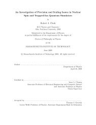
Figure 2.1: The velocity distribution for supersonic and effusive beams are compared<br />
for Helium and Neon beams at reservoir temperatures <strong>of</strong> 300 K and 77 K. The<br />
distributions are normalized to aid the comparison <strong>of</strong> flux at a particular velocity.<br />
The temperatures <strong>of</strong> the supersonic beams are taken from experimental data from<br />
the UT supersonic valve and experiments performed in Uzi Even’s lab at Tel Aviv<br />
University [28].<br />
called the quitting surface. Since the beam is no longer collisional downstream <strong>of</strong> the<br />
quitting surface, finding the velocity distribution at the quitting surface is sufficient<br />
to characterize the beam. The velocity distribution can be modeled <strong>as</strong> an anisotropic<br />
Maxwellian<br />
<br />
m m<br />
p(v) =<br />
2πkBT 2πkBT⊥<br />
Normalized <strong>Supersonic</strong> Beam Flux<br />
Normalized <strong>Supersonic</strong> Beam Flux<br />
e − mv2 ⊥<br />
2k B T ⊥ − m(v −w) 2<br />
2k B T , (2.24)<br />
where T and T⊥ are the temperatures along the axis <strong>of</strong> the beam and perpendicular<br />
to the beam respectively, <strong>with</strong> the same notation used for v and v⊥.<br />
In practice, the perpendicular temperature manifests <strong>as</strong> a loss <strong>of</strong> flux, since the<br />
beam generally goes through several apertures before being used in an experiment.<br />
14
The apertures set the transverse temperature, and hotter atoms are removed from the<br />
beam by the apertures, leaving only the colder atoms in the beam. For this re<strong>as</strong>on,<br />
it is appropriate to concentrate on the parallel component <strong>of</strong> the velocity, giving the<br />
Gaussian velocity pr<strong>of</strong>ile<br />
<br />
m<br />
p(v) = e<br />
2πkBT<br />
− m(v<br />
<br />
−w) 2<br />
2kB T<br />
=<br />
σ<br />
1<br />
√ e<br />
2π −(v <br />
−w) 2<br />
2σ 2 , (2.25)<br />
where σ is the standard deviation in the velocity parallel to the beam axis. This<br />
velocity distribution is compared to the Maxwellian velocity distribution for a few<br />
relevant g<strong>as</strong> species and reservoir temperatures in figure 2.1. As can be seen in<br />
the figure, the width <strong>of</strong> the velocity pr<strong>of</strong>ile is significantly narrower for the c<strong>as</strong>e <strong>of</strong><br />
a supersonic beam. Expressed in terms <strong>of</strong> temperature, beams <strong>of</strong> a few tens to a<br />
few hundred milliKelvin are common. This is significantly colder than the reservoir<br />
temperatures, and the supersonic expansion h<strong>as</strong> effectively cooled the beam.<br />
The cooling achieved by supersonic expansion is extremely general and can be<br />
used to cool any desired species. In the above discussion on isotropic expansion, it is<br />
<strong>as</strong>sumed that the g<strong>as</strong>es were truly ideal g<strong>as</strong>es. <strong>Supersonic</strong> beams are generally created<br />
<strong>with</strong> a noble carrier g<strong>as</strong> that generally behaves <strong>as</strong> an ideal g<strong>as</strong> at higher pressures<br />
and lower temperatures than many other g<strong>as</strong> species. Other species <strong>of</strong> interest are<br />
mixed in the reservoir before the expansion, or added just outside the nozzle during<br />
the expansion. If the species <strong>of</strong> interest is a g<strong>as</strong> at the reservoir temperature, it is<br />
typically seeded into the carrier g<strong>as</strong> in the reservoir. A species that is not a g<strong>as</strong> at the<br />
reservoir temperature is typically entrained into the beam at the exit <strong>of</strong> the nozzle.<br />
L<strong>as</strong>er ablation can be used to produce an atomic sample <strong>of</strong> a solid at the exit <strong>of</strong> a<br />
nozzle, or alternatively, an oven can produce an atomic beam that is then entrained in<br />
the supersonic beam. In either c<strong>as</strong>e, the added species is cooled by thermalizing <strong>with</strong><br />
the dominant carrier g<strong>as</strong> and is carried along <strong>with</strong> the supersonic beam, providing a<br />
15
general method for producing cold atoms.<br />
Different carrier g<strong>as</strong>es have their own advantages and disadvantages that must<br />
be weighed when selecting a species to use in an experiment. The m<strong>as</strong>s term in<br />
equation 2.23 means that a heavier carrier g<strong>as</strong> will produce a slower beam. This can<br />
be a large advantage, since supersonic beam velocities can range from several hundred<br />
to over a thousand meters per second. There are, however, some disadvantages to<br />
using heavier atoms <strong>as</strong> the carrier g<strong>as</strong>. Due to the dynamics <strong>of</strong> the collisions in the<br />
beam, light atoms being carried by a heavier carrier g<strong>as</strong> will tend to be pushed to the<br />
edges <strong>of</strong> the beam, and so the centerline flux <strong>of</strong> the species <strong>of</strong> interest will be reduced.<br />
The other possible disadvantage <strong>of</strong> a heavier carrier g<strong>as</strong> is the possibility <strong>of</strong> a hotter<br />
beam due to clustering. The binding energy <strong>of</strong> a cluster is rele<strong>as</strong>ed <strong>as</strong> heating in<br />
the beam itself. The cluster fraction can be estimated using the Hagena parameter<br />
[29, 30], and clustering becomes incre<strong>as</strong>ingly likely for the heavier noble g<strong>as</strong>es.<br />
2.3 The Even-Lavie Nozzle for Generating Pulsed <strong>Beams</strong><br />
The experiments described by this dissertation all use a pulsed valve for gener-<br />
ating supersonic beams [31–33]. The valves used are made by Uzi Even and Nachum<br />
Lavie at Tel Aviv University. There are several advantages to using a pulsed valve.<br />
The methods used to control the beams are pulsed and having a pulsed beam matches<br />
well <strong>with</strong> the control mechanisms. Additionally, the vacuum pumping requirements<br />
are significantly reduced by using a pulsed beam. Instead <strong>of</strong> using large diffusion<br />
pumps to maintain vacuum in the valve chamber, the experiments are able to use<br />
turbomolecular pumps that cannot contaminate the chamber <strong>with</strong> pump oils the way<br />
a diffusion pump can.<br />
The Even-Lavie uses a nozzle <strong>with</strong> a 200 μm diameter and a trumpet shaped<br />
expansion region. This shape helps to remove hot spots in the beam and reduces<br />
16
Figure 2.2: A CAD representation <strong>of</strong> the Even-Lavie supersonic nozzle. The complete<br />
nozzle apparatus is shown in (a) <strong>with</strong> a pool type cryostat which allows the nozzle<br />
to be cooled. G<strong>as</strong> flows into the valve apparatus through the stainless steel tube on<br />
the right side <strong>of</strong> the image into a stainless steel pressure tube (yellow). The front and<br />
back <strong>of</strong> the tube are sealed using Dupont Kapton w<strong>as</strong>hers (red). The trumpet shaped<br />
nozzle where the g<strong>as</strong> expands and exits is on the left. An empty section can be seen<br />
surrounding the stainless steel pressure tube, and this is where the electromagnetic<br />
drive coil (not shown in this image) is located. The interior <strong>of</strong> the pressure tube is<br />
shown in (b). G<strong>as</strong> enters the pressure tube (yellow) from the right and flows p<strong>as</strong>t<br />
the plunger (green), spring (blue), and guiding ceramic inserts (orange) to the nozzle<br />
exit (not depicted). The plunger forms a seal on the left side <strong>of</strong> the image <strong>with</strong><br />
the leftmost Kapton w<strong>as</strong>her from (a), and is held in place by the spring. Current<br />
in an electromagnetic coil produces a magnetic field that pulls the plunger to the<br />
right, allowing g<strong>as</strong> to expand adiabatically into the vacuum until the magnetic field<br />
is turned <strong>of</strong>f and the plunger is pushed back into place by the spring. The motion <strong>of</strong><br />
the plunger is guided by the two alumina pieces. Figure Courtesy Max Riedel.<br />
1/8’’<br />
the overall temperature, <strong>as</strong> well <strong>as</strong> producing a very directional beam <strong>with</strong> a FWHM<br />
opening angle <strong>of</strong> 16 ◦ [33]. The nozzle is unique in that it can produce pulses which<br />
are only 10 μs FWHM in length, and the valve can operate at repetition rates over<br />
40 Hz. The valve can operate <strong>with</strong> backing pressures <strong>of</strong> 100 atm and at temperatures<br />
<strong>as</strong> low <strong>as</strong> 20 K. The short opening time is essential for these reservoir conditions, <strong>as</strong><br />
the vacuum system would be overwhelmed by the resulting g<strong>as</strong> load otherwise.<br />
17
The g<strong>as</strong> throughput <strong>of</strong> the nozzle can be estimated by<br />
Φ= n0w<br />
4<br />
(2.26)<br />
where Φ is the throughput in molecules/m2 /s, n0 is the number density <strong>of</strong> the<br />
molecules in the reservoir, and w is the speed <strong>of</strong> the flow. Consider neon at 77 K<br />
<strong>with</strong> a reservoir pressure <strong>of</strong> 5 atm <strong>as</strong> an example. At this pressure and temperature,<br />
the ideal g<strong>as</strong> law (equation 2.1) gives a number density <strong>of</strong> 5 · 10 26 molecules/m 3 .The<br />
velocity <strong>of</strong> such a flow is approximately 400 m/s giving an estimated throughput <strong>of</strong><br />
5 · 10 28 molecules/m 2 /s. Using a nozzle opening time <strong>of</strong> 10 μs and accounting for the<br />
200 μm diameter <strong>of</strong> the valve gives a flux <strong>of</strong> 1.5 · 10 16 molecules/shot. Operating the<br />
valve under optimal conditions results in a peak brightness <strong>of</strong> 4 · 10 23 molecules/sr/s<br />
[33], which is greater than other sources [34–36] by at le<strong>as</strong>t an order <strong>of</strong> magnitude.<br />
A CAD representation <strong>of</strong> the valve is shown in figure 2.2. The nozzle hangs<br />
fromapooltypecryostatthatallowsthenozzletobecooled.The200μm diameter<br />
trumpet shaped nozzle is depicted on the left side <strong>of</strong> figure 2.2 (a), <strong>with</strong> the g<strong>as</strong><br />
entering from the stainless steel tube on the right. The g<strong>as</strong> flows through stainless<br />
steel pressure tube that is sealed at both ends by DuPont Kapton w<strong>as</strong>hers. The<br />
actual valve mechanism is depicted in figure 2.2 (b). The plunger forms a seal <strong>with</strong><br />
the Kapton w<strong>as</strong>her on the valve exit side <strong>of</strong> the high pressure tube and is held in<br />
place by a spring which sits inside the pressure tube. The plunger is moved by<br />
≈150 μm via an electromagnetic coil that produces fields <strong>of</strong> around 2.5 T, allowing<br />
g<strong>as</strong> to adiabatically expand into the vacuum. The plunger is guided by two alumina<br />
pieces that keep it centered in the pressure tube. The plunger is returned to the<br />
sealing position by the spring when the coil is turned <strong>of</strong>f. The entire plunger cycle<br />
takes 15 μs [37].<br />
The Even-Lavie valve is a good match for the experiments described in the<br />
remainder <strong>of</strong> this dissertation. The methods <strong>of</strong> slowing and control described here<br />
18
are pulsed methods, and cannot operate on a continuous b<strong>as</strong>is. As such, the pulsed<br />
source provided by the Even-Lavie valve limits the amount <strong>of</strong> w<strong>as</strong>ted g<strong>as</strong> rele<strong>as</strong>ed<br />
into the vacuum chamber. The uniquely short pulse lengths that the valve is capable<br />
<strong>of</strong> producing also provide a precise start time for the slowing experiments, permitting<br />
a simplification in the control electronics. Finally, since the overall goal <strong>of</strong> these<br />
experiments is to produce cold atoms that can be used for precision me<strong>as</strong>urements,<br />
the high beam brightness produced by the Even-Lavie valve is an important <strong>as</strong>set, <strong>as</strong><br />
this maximizes the number <strong>of</strong> atoms available.<br />
19
Chapter 3<br />
Slowing <strong>Supersonic</strong> <strong>Beams</strong> via Specular Reflection:<br />
The Atomic Paddle<br />
As experimental control <strong>of</strong> atomic motion h<strong>as</strong> improved, the wave nature <strong>of</strong><br />
atomic beams h<strong>as</strong> become an important factor in many experiments. Quantum me-<br />
chanics states that like light, matter is both a particle and a wave. This h<strong>as</strong> given<br />
birth to a new cl<strong>as</strong>s <strong>of</strong> experiments which exploit the wave nature <strong>of</strong> atoms and ma-<br />
nipulate beams <strong>of</strong> atoms in a particle analog to optical manipulation <strong>of</strong> beams <strong>of</strong><br />
light. This growing field is known <strong>as</strong> atom optics, and much research h<strong>as</strong> recently<br />
gone into developing a toolbox for manipulating atomic beams.<br />
Most <strong>of</strong> the work in atom optics h<strong>as</strong> used l<strong>as</strong>er cooled atoms [38, 39], which<br />
provide several advantages. Since the atoms are l<strong>as</strong>er cooled they are quite cold, and<br />
beams can be produced at low velocities. This accentuates the wave nature <strong>of</strong> the<br />
particles, <strong>as</strong><br />
λ = 2π<br />
(3.1)<br />
p<br />
where λ is the de Broglie wavelength <strong>of</strong> a particle, and p is the particle’s momentum.<br />
Furthermore, l<strong>as</strong>er cooled atoms have an accessible transition an experimentalist can<br />
use to both manipulate and detect the atoms in the beam. There are some drawbacks<br />
to using l<strong>as</strong>er cooled atoms however, most notably their sensitivity to stray fields.<br />
It is rather difficult to effectively control the atomic motion <strong>of</strong> ground state<br />
helium, due to the lack <strong>of</strong> accessible transitions <strong>with</strong> current l<strong>as</strong>er technology. How-<br />
ever, helium is known to reflect well from single crystal surfaces [40], which suggests<br />
20
a method by which beams <strong>of</strong> helium may be controlled. In the experiment described<br />
here, specular reflection from receding single crystal surfaces is used to control the<br />
velocity <strong>of</strong> a supersonic beam <strong>of</strong> helium atoms. The crystal is mounted on the tip<br />
<strong>of</strong> a spinning rotor that provides the necessary crystal velocity to effectively slow the<br />
beam. The original concept for this experiment w<strong>as</strong> first proposed by Doak [41], but<br />
the design studied had an expected slow beam flux that is significantly lower than in<br />
the experiment described here. The work presented in this chapter is also described<br />
in [33, 42, 43].<br />
The slower itself is similar to the beam paddle that w<strong>as</strong> developed for neutrons<br />
[44]. For helium atoms reflecting from a linearly moving single crystal surface, the<br />
velocity <strong>of</strong> the atoms after hitting the mirror will be<br />
vf = −vi +2vm, (3.2)<br />
where vf is the final velocity <strong>of</strong> the atoms, vi is the initial velocity <strong>of</strong> the incoming<br />
beam, and vm is the velocity <strong>of</strong> the mirror. The mirror is <strong>as</strong>sumed to be perpendicular<br />
to the incoming beam. Since the typical velocity <strong>of</strong> a supersonic beam is 500 m/s,<br />
reducing the velocity <strong>of</strong> the beam by a factor <strong>of</strong> two requires a crystal velocity <strong>of</strong><br />
125 m/s. While it is possible to create a device to repeatably move a mirror linearly<br />
at these speeds (perhaps by mounting the mirror on a projectile and launching and<br />
catching it using electromagnetic coils), it is simpler to let rotary motion approximate<br />
linear motion and mount the crystal on the tip <strong>of</strong> a spinning rotor arm. This facilitates<br />
the high mirror velocities required to significantly slow the beam. The introduction<br />
<strong>of</strong> rotary motion complicates equation 3.2, and the full description <strong>of</strong> the velocity<br />
change due to an atom reflecting from the rotor is shown in appendix A.<br />
21
3.1 Using Helium for Atom Optics <strong>Experiments</strong><br />
Most atom optics experiments have been done <strong>with</strong> l<strong>as</strong>er cooled atoms. The<br />
advantage <strong>of</strong> this is a cold sample which can e<strong>as</strong>ily be manipulated. However, be-<br />
cause <strong>of</strong> the large polarizability <strong>of</strong> most l<strong>as</strong>er coolable atoms, they are sensitive to<br />
stray electric fields. Similarly, many l<strong>as</strong>er coolable atoms are quite sensitive to stray<br />
magnetic fields. While their sensitivity is an advantage when controlling the atoms,<br />
stray fields will add systematic effects limiting the sensitivity <strong>of</strong> many me<strong>as</strong>urements.<br />
Though ground state noble g<strong>as</strong>es are difficult to manipulate, doing so is not<br />
impossible and there are several advantages to using them for experiments in atom<br />
optics. One such advantage is that they are known to reflect well from single crystal<br />
surfaces, and even if they do not reflect from a surface, they are unlikely to stick<br />
to it. Because <strong>of</strong> this, an aperture will not clog when subjected to a beam <strong>of</strong> noble<br />
g<strong>as</strong>es, even at high intensity. The other principle advantage is their low polarizabilty.<br />
Ground state noble g<strong>as</strong>es are relatively insensitive to stray electric fields, and they are<br />
insensitive to magnetic fields to first order. This makes ground state noble g<strong>as</strong>es, and<br />
ground state helium in particular, very attractive for certain precision me<strong>as</strong>urements<br />
and applications such <strong>as</strong> atom interferometry.<br />
A final advantage which is available when using ground state noble g<strong>as</strong>es for<br />
atom optics experiments is the large fluxes available. <strong>Supersonic</strong> beams typically use<br />
noble g<strong>as</strong>es <strong>as</strong> carriers, and a significant fraction <strong>of</strong> the flux <strong>of</strong> nearly any supersonic<br />
beam will consist <strong>of</strong> a ground state noble g<strong>as</strong>. Fluxes <strong>of</strong> up to 4 · 10 23 molecules/sr/s<br />
have been me<strong>as</strong>ured for pulsed beams <strong>as</strong> described in chapter 2, and for continuous<br />
beams, fluxes <strong>of</strong> 1.1 · 10 20 molecules/sr/s have been observed [45]. These bright-<br />
nesses provide a large advantage and can reduce the uncertainty <strong>of</strong> many precision<br />
me<strong>as</strong>urements, particularly for atom interferometry where the shot noise contributes<br />
significantly to the uncertainly. Helium is the atom most resistant to clustering, re-<br />
22
sulting in the brightest supersonic beams and providing further motivation to find<br />
methods <strong>of</strong> controlling ground state helium beams.<br />
In large part because <strong>of</strong> the advantages described above, there is a long history<br />
<strong>of</strong> using helium beams and helium scattering <strong>as</strong> an experimental probe. Stern and<br />
Estermann used helium diffraction from lithium fluoride crystals to demonstrate the<br />
wave nature <strong>of</strong> atoms and to experimentally confirm equation 3.1 [46]. Detailed<br />
examination <strong>of</strong> the diffraction <strong>of</strong> helium from surfaces h<strong>as</strong> provided many insights into<br />
the details <strong>of</strong> surface structure and the atom-surface potential [47]. More recent work<br />
h<strong>as</strong> used transmission diffraction gratings to study helium clustering in supersonic<br />
beams [35].<br />
While ground state noble g<strong>as</strong>es are more difficult to control than atoms which<br />
are l<strong>as</strong>er coolable, several techniques have been developed which can be applied to<br />
the control <strong>of</strong> ground state helium. A standard optical toolbox includes mirrors,<br />
beamsplitters, and lenses. To effectively use ground state helium for atom optics,<br />
analogs <strong>of</strong> these tools are required. One such approach to creating these tools h<strong>as</strong><br />
been to use species independent methods such <strong>as</strong> transmission diffraction gratings<br />
[48–50] and transmission Fresnel lenses [51, 52]. Another approach is to make use <strong>of</strong><br />
the high el<strong>as</strong>tic scattering probability <strong>of</strong> helium from crystal surfaces. Flat surfaces<br />
create mirrors and the equivalent <strong>of</strong> a lens can be formed by bending the crystal,<br />
creating a curved mirror [12]. Finally, the periodic structure <strong>of</strong> a crystal surface can<br />
be used <strong>as</strong> a diffraction grating [53], creating a beamsplitter for the atoms. In this<br />
manner, the entire optical toolbox can be created using crystal surfaces.<br />
3.2 Reflecting <strong>Atoms</strong> from Surfaces: Atomic Mirrors<br />
Having a large fraction <strong>of</strong> the helium beam be el<strong>as</strong>tically scattered from the<br />
crystal surface is important when manipulating a supersonic beam using reflection<br />
23
Figure 3.1: Calculated el<strong>as</strong>tic scattering probability for helium incident on Si(111) for<br />
different beam velocities <strong>as</strong> a function <strong>of</strong> crystal temperature. These are calculated<br />
using the Debye-Waller factor described in equations 3.3 and 3.4. While the el<strong>as</strong>tic<br />
fraction is well approximated by the Debye-Waller factor, atoms may still be diffracted<br />
and these numbers do not represent the fraction <strong>of</strong> specularly reflected atoms. Figure<br />
Courtesy Max Riedel.<br />
from crystals. Assuming the atom surface potential h<strong>as</strong> zero well depth (which means<br />
that there is no Beeby correction), the el<strong>as</strong>tic scattering fraction from single crystalline<br />
surfaces is governed by the Debye-Waller factor [54],<br />
I<br />
I0<br />
= e −2W<br />
where I is the el<strong>as</strong>tically reflected intensity, I0 is the incident intensity, and<br />
(3.3)<br />
W = 12mE⊥Ts<br />
MkBθ2 . (3.4)<br />
s<br />
Here m is the m<strong>as</strong>s <strong>of</strong> the incident atom, E⊥ is the incident energy, Ts is the temper-<br />
ature <strong>of</strong> the crystal, M is the m<strong>as</strong>s <strong>of</strong> the atom in the crystal, and θs is the Debye<br />
temperature <strong>of</strong> the crystal.<br />
24
To put equations 3.3, and 3.4 into context, consider the following example.<br />
The experiment uses Si(111) <strong>as</strong> the reflecting surface, for re<strong>as</strong>ons described in section<br />
3.2.1, and the following calculation is b<strong>as</strong>ed on this surface. The average m<strong>as</strong>s <strong>of</strong> a<br />
single silicon atom in the crystal is 4.7 · 10 −26 kg and the crystal Debye temperature is<br />
690K (at room temperature). For a supersonic beam <strong>of</strong> helium from a 77K nozzle, the<br />
beam velocity is ≈ 900m/s and the m<strong>as</strong>s <strong>of</strong> a helium atom is 6.7·10 −27 kg. From this,<br />
the Debye-Waller factor indicates that 65% <strong>of</strong> the beam will be el<strong>as</strong>tically scattered.<br />
While this is a good approximation <strong>of</strong> the el<strong>as</strong>tic scattering amplitude, it does not<br />
indicate the fraction <strong>of</strong> the beam which will be specularly reflected, <strong>as</strong> the beam may<br />
be distributed into many diffraction channels. Figure 3.1 shows what fraction <strong>of</strong> a<br />
helium beam will be el<strong>as</strong>tically scattered <strong>as</strong> a function <strong>of</strong> crystal temperature, for<br />
several incident beam velocities.<br />
3.2.1 Crystal Choice: Si(111)<br />
The choice <strong>of</strong> crystal substrate is important when creating a good atomic mir-<br />
ror. Ideally, an atomic mirror will be atomically flat, since diffuse scattering will<br />
result from surfaces that are rough on a length scale above the wavelength <strong>of</strong> the<br />
incident beam. Also, since a mirror requires high specular reflection, the crystal sub-<br />
strate should have a high Debye temperature, <strong>as</strong> well <strong>as</strong> low surface corrugation to<br />
minimize diffracted flux. Additionally, the surface must be stable against reconstruc-<br />
tion and corrosion, and will ideally be p<strong>as</strong>sive, reducing the accumulation <strong>of</strong> dirt and<br />
adsorbates on the surface that lower the specularly reflected intensity. Finally, the<br />
surface needs to be simple and inexpensive to prepare.<br />
Crystal surfaces for helium diffraction studies are typically prepared by cleav-<br />
ing or annealing in-situ. Because the crystal must be mounted to the tip <strong>of</strong> a rotor,<br />
these methods are not ideal for this experiment. However, some surfaces are so inert<br />
25
that they can be prepared ex-situ and will remain clean enough to still reflect helium<br />
well. The crystal chosen for this experiment, is hydrogen p<strong>as</strong>sivated Si(111). Lithium<br />
fluoride w<strong>as</strong> also examined <strong>as</strong> a possible crystal substrate, and the details <strong>of</strong> this<br />
examination may be found in [55].<br />
To use Si(111) <strong>as</strong> an atomic mirror which is prepared ex-situ, thecrystalmust<br />
be p<strong>as</strong>sivated. A freshly cleaved Si(111) surface will have dangling bonds and the<br />
surface will not be p<strong>as</strong>sive enough to keep contaminants from sticking to the surface.<br />
By wet etching the surface, the dangling bonds are terminated <strong>with</strong> hydrogen, which<br />
p<strong>as</strong>sivates the surface, resulting in Si(111)-(1×1)H [56, 57]. The mirrors are created<br />
from phosphor doped 200μm thick wafers <strong>with</strong> a pre-existing oxide layer and a miscut<br />
angle <strong>of</strong> ±0.1 ◦ acquired from Virginia Semiconductor. The 100 mm diameter waferes<br />
were pre-cut into smaller circles [58], but the cutting process scratched the crystal<br />
surfaces and rendered the area <strong>with</strong>in 2 mm <strong>of</strong> a cut unusable. The wafers are cut to<br />
their final size for etching and insertion into the vacuum chamber by a dicing saw,<br />
removing the damaged regions. The wet etching process used to create this surface<br />
is now described.<br />
3.2.2 Crystal Preparation and Wet Etching<br />
To produce an atomically flat p<strong>as</strong>sivated Si surface, the crystal must first be<br />
cleaned <strong>as</strong> much <strong>as</strong> possible to remove contaminants, especially organic residues. The<br />
procedure described below is b<strong>as</strong>ed on suggestions from the group <strong>of</strong> Dr. Ken Shih at<br />
The University <strong>of</strong> Tex<strong>as</strong> at Austin, and the group <strong>of</strong> Dr. Bill Allison at the Cavendish<br />
Lab in Cambridge [57]. All chemicals used are LP grade or better, and the ammonium<br />
fluoride is MB grade. Additionally, any water used in the procedure is ultra pure and<br />
h<strong>as</strong> a resistivity <strong>of</strong> greater than 17 MΩ cm. Finally, all beakers, bottles, containers,<br />
and tools used to handle the wafers or in contact <strong>with</strong> the chemicals are made <strong>of</strong><br />
26
PTFE or PFA. The procedure takes place under the fume hood, and the working<br />
surface is covered by a layer <strong>of</strong> clean room wipes.<br />
The initial cleaning is done by sonicating the crystal in isopropanol for 10<br />
minutes, followed by another 10 minutes in acetone. The crystals are then rinsed <strong>with</strong><br />
water to remove these organic solvents before continuing the cleaning process. The<br />
next step is to place the wafers in an RCA I solution which removes organic residues<br />
and grows a uniform oxide layer. This solution consists <strong>of</strong> 1 part 30% ammonium<br />
hydroxide, 1 part 30 % hydrogen peroxide, and 5 parts water. The water is heated<br />
in a water bath on a hot plate to 80 ◦ C and the ammonium hydroxide and hydrogen<br />
peroxide are added just before the wafers. The solution is stirred gently <strong>with</strong> a<br />
magnetic stirrer on the hot plate. The crystal is left in the RCA I solution for 5<br />
minutes, at which point it is removed from the solution and rinsed <strong>with</strong> water. Each<br />
rinsing step described here involves a significant quantity <strong>of</strong> water, typically at le<strong>as</strong>t<br />
half a liter is poured over each crystal during the rinsing ph<strong>as</strong>es.<br />
The next step is the wet etching, which is done in a 40 % solution <strong>of</strong> ammonium<br />
fluoride. Before the crystals are etched, the disolved oxygen in the ammonium fluoride<br />
must first be removed by bubbling ultra pure argon through the solution for at le<strong>as</strong>t<br />
40 minutes prior to inserting the crystals. For the crystals used here, etch times<br />
between 10 and 15 minutes are optimal. Shorter times do not completely remove the<br />
surface oxide layer, while longer times result in deep etch pits in the surface. The<br />
crystals used in the experiments described below are etched for 12 minutes. Unlike<br />
in the previous steps, the ammonium fluoride solution is not stirred or disturbed in<br />
any way while etching the crystals. Even continuing to gently bubble argon in the<br />
solution negatively affects the resulting surface.<br />
After the etching is complete, the crystal is rinsed a final time. The p<strong>as</strong>sivated<br />
surface is hydrophobic, and the water does not wet the surface if the etching is<br />
27
successful. Any water that remains on the crystal can be removed by blowing it <strong>of</strong>f<br />
<strong>with</strong> argon. Storing the crystal in an argon environment until it can be inserted into<br />
vacuum preserves the pristine state <strong>of</strong> the surface.<br />
3.2.3 Crystal Characterization<br />
To characterize the p<strong>as</strong>sivated surfaces, they are examined using an atomic<br />
force microscope (AFM). The AFM is operated in tapping mode, and scanning 2μmby<br />
2μm regions <strong>of</strong> the wafer w<strong>as</strong> found to provide a good compromise between examining<br />
a large area and scan speed. Figure 3.2 shows AFM images <strong>of</strong> a wafer that w<strong>as</strong> wet<br />
etched. Image (a) shows a clean surface, <strong>with</strong> large atomically flat regions. The steps<br />
seen in the image are bilayer steps from one crystal plane to another, and are 3.8 ˚A<br />
high. The image is <strong>of</strong> the wafer 15 minutes after removing it from the etching solution.<br />
Image (b) shows the same wafer after waiting an additional 28 minutes. The apparent<br />
incre<strong>as</strong>e in surface roughness is likely due to the oxidation <strong>of</strong> the crystal. The height<br />
pr<strong>of</strong>iles shown in images (c) and (d) are taken along the white lines shown in (a) and<br />
(b) respectively. The surface roughness shown in (c) is less than an ˚A in magnitude,<br />
and is probably noise in the AFM rather than real artifacts on the crystal surface.<br />
However, the incre<strong>as</strong>ed surface roughness shown in (d) shows grains approximately 2˚A<br />
in height, and is likely showing real contamination <strong>of</strong> the surface. This indicates the<br />
importance <strong>of</strong> minimizing the time the crystals spend in atmosphere before inserting<br />
them into the vacuum chamber.<br />
3.3 The Experimental Apparatus<br />
This section describes the apparatus constructed to create, slow, and detect<br />
a beam <strong>of</strong> supersonic helium. The description <strong>of</strong> the apparatus follows the path <strong>of</strong><br />
the beam, starting <strong>with</strong> the vacuum system, followed by the slowing apparatus, and<br />
28
(c) (d)<br />
Figure 3.2: An AFM image <strong>of</strong> a p<strong>as</strong>sivated Si(111) crystal. Image (a) and (b) are<br />
2 μm by2μm regions <strong>of</strong> the same wafer, 15 minutes and 43 minutes after etching<br />
respectively. Image (a) shows atomically flat regions separated by bilayer steps between<br />
crystal planes, each <strong>of</strong> which are 3.8 ˚A high. The incre<strong>as</strong>ed noise seen in image<br />
(b) shows the surface contamination (most likely oxidation) from the additional 28<br />
minutes the wafer spent in atmosphere. The height pr<strong>of</strong>iles shown in (c) and (d) are<br />
taken along the white lines in (a) and (b) respectively. The roughness <strong>of</strong> the crystal<br />
terraces in (a) and (c) are likely noise in the AFM, but the incre<strong>as</strong>ed roughness seen in<br />
(b) and (d), showing grains approximately 2˚A high, show the incre<strong>as</strong>ed contamination<br />
<strong>of</strong> the surface.<br />
29
Skimmer<br />
300 l/s Turbo Pump<br />
Even-Lavie<br />
<strong>Supersonic</strong><br />
Nozzle<br />
300 l/s Turbo Pump<br />
Figure 3.3: A CAD image <strong>of</strong> the nozzle chamber. The chamber is pumped by two<br />
300 l/s turbo pumps (indicated). The Even-Lavie nozzle hangs from a pool type<br />
cryostat into the center <strong>of</strong> the right 6 inch cross (the beam propagates left in this<br />
image). The skimmer h<strong>as</strong> a 5 mm aperture and is 5 cm long and sits ≈ 30 cm from<br />
the nozzle.<br />
finally a description <strong>of</strong> the detection system and experimental control system.<br />
3.3.1 The Vacuum System<br />
The vacuum system for this experiment is divided into three distinct sections,<br />
the beam creation chamber, the rotor chamber, and the detection chamber. The<br />
beam creation chamber consists <strong>of</strong> one 4-way 6 inch cross, and one 6-way 6 inch cross.<br />
These were purch<strong>as</strong>ed from HPS [59] and are custom made to have a tolerance <strong>of</strong><br />
.5 ◦ in parallelism and perpendicularity <strong>of</strong> the flanges, and are constructed to .02 inch<br />
tolerances. These tolerances ensures that the Even-Lavie nozzle sits in the center <strong>of</strong><br />
the chamber and that the beam propagates along the center-line <strong>of</strong> the chambers.<br />
An image <strong>of</strong> the beam creation chamber <strong>with</strong> the Even-Lavie valve is shown<br />
in figure 3.3. The chamber is pumped by two 300 l/s Leybold turbo pumps, which<br />
maintain a pressure <strong>of</strong> 10 −6 torr when the nozzle is operating at a repetition rate<br />
30
500 l/s Turbo<br />
Pump<br />
<strong>Cold</strong> Cathode<br />
Vacuum Gauge<br />
Helium<br />
Beam<br />
Figure 3.4: A CAD image <strong>of</strong> the rotor chamber. The chamber is pumped by a 500 l/s<br />
turbo pump (indicated). The chamber walls are 1 inch thick 304 stainless steel, and<br />
the chamber disc is 112cm in diameter and 12.7cm high.<br />
<strong>of</strong> 5 Hz (10 −8 torr when the nozzle is not operating). This is monitored by a cold<br />
cathode vacuum gauge (not shown). The nozzle hangs from a pool type cryostat into<br />
the center <strong>of</strong> the 6-way cross. The beam propagates 30cm to the 5cm skimmer, which<br />
h<strong>as</strong> a 5 mm aperture. From the skimmer, the beam p<strong>as</strong>ses into the rotor chamber,<br />
which is connected to the nozzle chamber by a flexible bellows, allowing the helium<br />
beam to be aligned to the rest <strong>of</strong> the experiment.<br />
The rotor chamber h<strong>as</strong> to accommodate the rotor, which is the key element<br />
in the design <strong>of</strong> the chamber <strong>as</strong> a whole. As described in section 3.3.2, the rotor is<br />
100.8 cm in diameter, and so the chamber needs to be large enough to allow it to spin<br />
freely. In addition, the beam needs to enter the interaction region and be detected.<br />
This led to a custom chamber design, <strong>as</strong> seen in figure 3.4. The chamber is pumped<br />
by a 500 l/s Varian turbo pump that keeps the chamber at a pressure <strong>of</strong> 2 · 10 −8 torr<br />
while the nozzle is firing (10 −9 torr when the nozzle is not operating). The chamber<br />
31
Figure 3.5: A CAD image <strong>of</strong> the detection chamber. The chamber is separated from<br />
the rotor chamber by a 5 mm aperture. This provides differential pumping, keeping<br />
the detection volume from experiencing too high a g<strong>as</strong> load from the direct beam.<br />
The chamber is pumped by a 70 l/s turbo pump. Figure Courtesy Max Riedel.<br />
is constructed from 1 inch thick stainless steel, and can be seen in figure 3.4. The<br />
chamber disc is 112 cm in diameter and 12.7 cm high. Due to the large surface area<br />
<strong>of</strong> the top and bottom <strong>of</strong> this disc, atmospheric pressure moves the top and bottom<br />
<strong>of</strong> the chamber together by 4 mm when the chamber is under vacuum.<br />
The final chamber section is the detection chamber, illustrated in figure 3.5.<br />
The detection chamber is separated from the rotor chamber by a 5 mm aperture<br />
constructed from a copper disc (used instead <strong>of</strong> an annular g<strong>as</strong>ket where the rotor<br />
chamber connects to the detection chamber). The detection chamber is pumped by<br />
a 70 l/s Varian turbo pump, and houses the detector used to observe the beam when<br />
it does not interact <strong>with</strong> the rotor. This detector is located 1.42 m from the nozzle.<br />
The direct beam detector w<strong>as</strong> originally directly connected to the rotor chamber, but<br />
this negatively impacted detector performance, probably due to the significant g<strong>as</strong><br />
load entering the detection region <strong>with</strong>out adequate pumping.<br />
The entire apparatus is shown in figure 3.6. The support structures are made<br />
32
Figure 3.6: A CAD image <strong>of</strong> the entire apparatus, including the chamber support<br />
structure and optical breadboards. The Even-Lavie nozzle and skimmer are shown in<br />
green, the SRS residual g<strong>as</strong> analyzers used to detect the beam are shown in blue, the<br />
rotor and spindle are shown in yellow, and the motor and rotary feedthrough which<br />
drive the rotor are shown in orange. Figure Courtesy Max Riedel.<br />
33
from tubular aluminum welded together to support the 600 kg chamber m<strong>as</strong>s. The<br />
Even-Lavie nozzle is shown in green, <strong>as</strong> is the skimmer and skimmer mount. The<br />
SRS residual g<strong>as</strong> analyzers used for beam detection are shown in blue. The rotor and<br />
spindle are depicted in yellow, while the rotary feedthrough and motor which drive<br />
the rotor are shown in orange.<br />
3.3.2 The Rotor<br />
There are several design requirements for the rotor itself, which informed its<br />
final construction. As can be seen from equation 3.2, to significantly slow a supersonic<br />
beam, the crystal should be capable <strong>of</strong> reaching velocities up to half <strong>of</strong> the initial beam<br />
speed. A supersonic beam <strong>of</strong> pure helium from a nozzle cooled <strong>with</strong> liquid nitrogen to<br />
77 K will have a velocity <strong>of</strong> 900 m/s and so the rotor w<strong>as</strong> originally designed to reach<br />
tip velocities <strong>of</strong> up to 450m/s. Another design constraint comes from the use <strong>of</strong> rotary<br />
motion to approximate linear motion <strong>of</strong> the crystal. Clearly, over small distances, a<br />
larger rotor will more closely approximate linear motion. This is important because<br />
the helium beam h<strong>as</strong> a finite spatial and temporal extent when it arrives at the crystal<br />
(≈ 100 μs). The angle <strong>of</strong> reflection changes during the arrival <strong>of</strong> the beam, limiting<br />
the fraction <strong>of</strong> the reflected beam which travels in the desired direction. This fanning<br />
effect leads to a loss <strong>of</strong> flux, and should ideally be minimized by making the rotor <strong>as</strong><br />
large <strong>as</strong> practical. Finally, an effective and simple method <strong>of</strong> mounting the crystals<br />
to the tip <strong>of</strong> the rotor, which does not overly compromise the rotor’s strength, needs<br />
to be found.<br />
3.3.2.1 Initial Design<br />
The centripetal force needed to hold a m<strong>as</strong>s in circular motion, F = mv2<br />
r<br />
mω 2 r,whereF is the force, m is the m<strong>as</strong>s <strong>of</strong> the body, r is the radius <strong>of</strong> the orbit, v<br />
34<br />
=
is the velocity, and ω is the angular velocity, dictates the design <strong>of</strong> the rotor, which<br />
must be strong enough at every point to support the force exerted by the section <strong>of</strong><br />
the rotor at larger radius. The force at each position can be approximated (<strong>as</strong>suming<br />
no transverse forces in the rotor) <strong>as</strong><br />
F =<br />
rmax<br />
ρA(r)ω 2 rdr, (3.5)<br />
where rmax<br />
rc<br />
is the maximum radius <strong>of</strong> the rotor, rc is position the force is being<br />
me<strong>as</strong>ured, ρ is the density <strong>of</strong> the rotor material, and A(r) is the cross sectional area<br />
<strong>of</strong> the rotor. The force at each position must be compared to the yield tensile strength<br />
<strong>of</strong> the rotor material times the cross sectional area. Equation 3.5 shows that a light<br />
and strong material is ideal for the rotor. While composites would be ideal, their<br />
lack <strong>of</strong> vacuum compatibility poses a serious problem. The chosen rotor material is<br />
grade 5 titanium, a high strength alloy which is also vacuum compatible. Another<br />
constraint on the rotor design is the vacuum itself, since the rotor must fit into a<br />
practical vacuum chamber. This led to a compromise design <strong>with</strong> a rotor radius <strong>of</strong><br />
50.4 cm at the center <strong>of</strong> the crystal.<br />
A CAD image <strong>of</strong> the rotor can be seen in figure 3.7. The overall length <strong>of</strong> the<br />
rotor is 101.5 cm. Since the inside <strong>of</strong> the rotor needs to be stronger than the tips,<br />
<strong>as</strong> seen in equation 3.5, the rotor is tapered linearly from a minimum thickness <strong>of</strong><br />
0.3175cm where the rotor joins the mirror holder, to a maximum thickness <strong>of</strong> 2.54cm,<br />
<strong>with</strong> the rotor a constant thickness over its center 5.08 cm. This taper reduces the<br />
m<strong>as</strong>s at large radius, reducing the force exerted, while placing material where it is<br />
needed near the center <strong>of</strong> the rotor. The crystal mirrors, which fit directly into the<br />
rotor are 5 mm in diameter and are held in place by an aluminum set screw, allowing<br />
for an exposed crystal diameter <strong>of</strong> 4 mm.<br />
While an analytical calculation <strong>of</strong> the forces placed on a the rotor is pro-<br />
hibitively complex, finite element analysis permits a numerical calculation <strong>of</strong> the<br />
35
Figure 3.7: A CAD image <strong>of</strong> the rotor. The rotor h<strong>as</strong> 50.4 cm radius at the center <strong>of</strong><br />
the crystal holder, and a maximum thickness <strong>of</strong> 2.54 cm in the center. The diameter<br />
<strong>of</strong> the rotor itself is linearly tapered from 0.3175 cm where the rotor joins the crystal<br />
holder, to the maximal thickness 2.54 cm from the middle <strong>of</strong> the rotor. The small<br />
hole seen in the middle <strong>of</strong> the rotor allows precise centering <strong>of</strong> the rotor via a pin in<br />
the spindle. A 5 mm diameter crystal (4 mm exposed) is held in place by a set screw.<br />
Figure Courtesy Max Riedel.<br />
Figure 3.8: A finite element calculation <strong>of</strong> the stress exerted on the rotor by rotation<br />
at 140 Hz. This is expressed in MPa, since it is the force per unit area <strong>of</strong> material,<br />
rather than the absolute force, which is relevant. For reference, the peak stress place<br />
on the rotor is only a factor <strong>of</strong> 5 smaller than the yield tensile strength <strong>of</strong> the titanium<br />
alloy used.<br />
36
Figure 3.9: A CAD image <strong>of</strong> the rotor <strong>as</strong> held by the initial spindle. The spindle is<br />
rigidly coupled to the shaft <strong>of</strong> the ferr<strong>of</strong>luidic feedthrough. The feedthough attaches<br />
toa10− 4.5 inch zero length reducer, which supports the spinning parts, <strong>as</strong> well <strong>as</strong><br />
the motor, which is mounted above the feedthrough via a flexible coupling. Figure<br />
Courtesy Max Riedel.<br />
forces. Figure 3.8 shows a finite element calculation <strong>of</strong> the stresses placed on the ro-<br />
tor by rotation at 140 Hz, me<strong>as</strong>ured in MPa. This is expressed <strong>as</strong> a pressure because<br />
the strength <strong>of</strong> the material is proportional to the cross sectional area, and thus the<br />
relevant number is not the absolute force placed on the rotor, but rather the force<br />
per unit area. The maximum stress placed on the rotor by this speed <strong>of</strong> rotation is<br />
152 MPa, which is well below the yield tensile strength <strong>of</strong> the titanium allow used<br />
(880 MPa).<br />
The rotor is held in vacuum by a stainless steel spindle which is rigidly coupled<br />
to the shaft <strong>of</strong> a ferr<strong>of</strong>luidic rotary feedthrough [60]. Since an object will rotate stably<br />
around the axis <strong>of</strong> lowest or highest inertia, one goal in the construction <strong>of</strong> the spindle<br />
w<strong>as</strong> to ensure that the rotor would be spinning about the axis <strong>with</strong> the highest moment<br />
<strong>of</strong> inertia (the lowest moment being rotation about the centerline <strong>of</strong> the rotor itself).<br />
To do this, a disc w<strong>as</strong> added to the spindle, <strong>with</strong> most <strong>of</strong> the m<strong>as</strong>s on the outside<br />
37
Figure 3.10: A CAD image <strong>of</strong> large crystal holder attached to the rotor. This enables<br />
12.7 mm diameter crystals to be mounted to the rotor tips. The crystals are held<br />
between a threaded aluminum circular plate and a titanium locking ring, exposing a<br />
9 mm diameter region <strong>of</strong> the crystal. The circular plate connects via a threaded hole<br />
to an adapter, which fits in the rotor where the smaller crystals would sit. Figure<br />
Courtesy Max Riedel.<br />
<strong>of</strong> the disc. The spindle also h<strong>as</strong> screw holes drilled around the outside <strong>of</strong> the disc,<br />
which were added to allow for the balancing <strong>of</strong> the rotor and spindle should this be<br />
necessary. The rotating parts <strong>of</strong> the experiment, along <strong>with</strong> the 4−10inch zero length<br />
conflat reducer they are suspended from, are shown in figure 3.9.<br />
As is explained in section 3.3.2.2, the maximum speed <strong>of</strong> the rotor w<strong>as</strong> ini-<br />
tially limited to 42 Hz due to the vibrational stability <strong>of</strong> the spindle. Since the stress<br />
placed on the rotor scales quadratically <strong>with</strong> the rotation rate, being limited to 42 Hz<br />
reduced the expected stresses by an order <strong>of</strong> magnitude. This allowed the size <strong>of</strong> the<br />
crystal to be incre<strong>as</strong>ed, becau<strong>as</strong>e the rotor is strong enough support the incre<strong>as</strong>ed<br />
m<strong>as</strong>s <strong>of</strong> a larger crystal and crystal holder at the tip for these velocities. The larger<br />
crystal incre<strong>as</strong>es the area over which the beam can reflect from the rotor tip, incre<strong>as</strong>-<br />
ing the reflected flux. An image <strong>of</strong> the larger crystal holder can be seen in figure<br />
3.10. The larger crystal holder incre<strong>as</strong>es the diameter <strong>of</strong> the crystals from 5 mm to<br />
12.7 mm. These crystals are clamped between a threaded aluminum circular plate,<br />
38
and a titanium locking ring, <strong>with</strong> an exposed crystal diameter <strong>of</strong> 9 mm. The back <strong>of</strong><br />
the threaded plate h<strong>as</strong> a tapped hole, which screws onto a third piece which fits into<br />
the rotor via the smaller crystal mounting threads. This system h<strong>as</strong> the additional<br />
advantage <strong>of</strong> simplifying the mounting and removing <strong>of</strong> crystals from the rotor, re-<br />
ducing the time the crystals and the vacuum chamber are exposed to air during a<br />
crystal exchange.<br />
3.3.2.2 Vibration and Balancing<br />
The spinning parts <strong>of</strong> the experiment are all constructed <strong>with</strong> dimensional<br />
tolerances <strong>of</strong> .001 inches, which ensures that the rotor apparatus should be nearly<br />
balanced to begin <strong>with</strong>. To verify the initial balancing, the rotor w<strong>as</strong> mounted <strong>with</strong><br />
the motor axis horizontal, instead <strong>of</strong> vertical <strong>as</strong> it is in the chamber, and statically<br />
balanced. This provides the rough balancing needed to initially spin the rotor, since<br />
even a small static imbalance would lead to potentially large vibrations when spinning.<br />
To balance the spinning system, the vibration <strong>of</strong> the rotor must be me<strong>as</strong>ured.<br />
This is accomplished in two ways. The first method uses a l<strong>as</strong>er beam to me<strong>as</strong>ure<br />
the amplitude <strong>of</strong> the pendulum modes <strong>of</strong> the shaft. The l<strong>as</strong>er is directed though the<br />
chamber, <strong>with</strong> half <strong>of</strong> the beam blocked by the lower part <strong>of</strong> spindle. As the shaft<br />
vibrates, the spindle moves in the l<strong>as</strong>er beam, blocking more or less <strong>of</strong> the beam,<br />
which is detected by monitoring the intensity <strong>of</strong> the light leaving the chamber via a<br />
photo diode. Vibrations are detected to an accuracy <strong>of</strong> 5μm using this setup. A knife<br />
edge mounted to a micrometer is used to calibrate the readings. Having <strong>as</strong>sembled<br />
the system <strong>with</strong> the greatest accuracy possible, using feeler gauges to ensure that<br />
parts are properly aligned, a runout <strong>of</strong> 70 μm is observed (over the course <strong>of</strong> one slow<br />
rotation the spindle moves over a range <strong>of</strong> 70 μm).<br />
The second method <strong>of</strong> monitoring the vibrations does not directly me<strong>as</strong>ure<br />
39
Figure 3.11: This plot shows the amplitude <strong>of</strong> the rotor vibration at several rotational<br />
speeds. The vibrational amplitude me<strong>as</strong>ured by the l<strong>as</strong>er is shown in red, while the<br />
amplitude me<strong>as</strong>ured by the accelerometer outside the chamber is shown in black.<br />
The d<strong>as</strong>hed lines indicate observed resonances <strong>as</strong> observed by either the l<strong>as</strong>er or the<br />
accelerometer. The solid line is a Lorentzian fit for the resonance which ultimately<br />
limits the rotor velocity.<br />
the motion <strong>of</strong> the rotor, but instead monitors the vibrations which are transmitted<br />
to the chamber. This is done by rigidly mounting an accelerometer chip to the top<br />
<strong>of</strong> the vacuum chamber. While an externally mounted accelerometer cannot me<strong>as</strong>ure<br />
the amplitude <strong>of</strong> vibrations on the rotor, or determine the mode <strong>of</strong> vibration, it does<br />
have the advantage <strong>of</strong> detecting vibrational modes the l<strong>as</strong>er is insensitive to. The<br />
experiment is set up to monitor the level <strong>of</strong> vibration me<strong>as</strong>ured by the l<strong>as</strong>er and<br />
the accelerometer, and automatically spins down the rotor if the vibrations grow too<br />
large.<br />
The vibrations observed using these detection systems are significantly larger<br />
than anticipated when the rotor w<strong>as</strong> designed. A plot <strong>of</strong> vibrational amplitude for<br />
different rotation speeds is shown in figure 3.11. The plot shows the vibrational ampli-<br />
tude me<strong>as</strong>ured by the l<strong>as</strong>er in red, and the amplitude me<strong>as</strong>ured by the accelerometer<br />
40
Figure 3.12: Finite element calculation <strong>of</strong> rotor vibrational modes. This w<strong>as</strong> performed<br />
using the built in finite element package in Solid Edge. The vibrational mode<br />
shown h<strong>as</strong> a resonance frequency <strong>of</strong> 47Hz. The calculation does not take into account<br />
the fact that the rotor and spindle are made from different materials, <strong>as</strong> only one material<br />
can be simulated. As such the entire structure is simulated <strong>as</strong> stainless steel,<br />
since most <strong>of</strong> the weight is in the stainless steel spindle. Additionally, the shaft <strong>of</strong> the<br />
spindle, which is found to be region that flexes most, is stainless steel. Reducing the<br />
weight <strong>of</strong> the rotor (it is titanium in the experiment) would likely result in a slightly<br />
higher resonant frequency in the real system.<br />
in black. The d<strong>as</strong>hed lines indicate resonances by at le<strong>as</strong>t one <strong>of</strong> these methods. Ad-<br />
ditionally, these resonances can be heard <strong>as</strong> incre<strong>as</strong>ed noise from the chamber, and<br />
the chamber vibrations are e<strong>as</strong>ily felt by placing a hand on the chamber. The solid<br />
lines in figure 3.11 are Lorentzian fits <strong>of</strong> the limiting resonance, which is predicted<br />
be lie around 48 − 50 Hz. From these fits, the peak vibrational amplitude can be<br />
estimated to be 1000 − 2000 μm which is too large to be comfortably p<strong>as</strong>sed through,<br />
and thus limits the rotor velocity to 42 Hz.<br />
A finite element calculation <strong>of</strong> the vibrational modes <strong>of</strong> the rotor and spindle<br />
w<strong>as</strong> performed to investigate the source <strong>of</strong> this unexpected resonance using the built<br />
in finite element package <strong>of</strong> CAD program Solid Edge. This analysis shows the nature<br />
<strong>of</strong> the resonance which limits the rotor velocity, and the results <strong>of</strong> this calculation are<br />
shown in figure 3.12. The finite element calculation predicts two pendulum modes,<br />
one at 34 Hz and one at 47 Hz, in addition to a twisting mode at 35 Hz. Several<br />
41
approximations are made in this calculation. The first approximation is that the cou-<br />
pling between the spindle and feedthrough is truly rigid. The second approximation<br />
comes from the fact that this finite element package cannot simulate two materials<br />
simultaneously. The entire rotor structure is simulated <strong>as</strong> stainless steel, since the<br />
stainless steel spindle comprises most <strong>of</strong> the m<strong>as</strong>s, and because the point which the<br />
calculations indicate is flexing the most is the stainless steel shaft <strong>of</strong> the spindle. In<br />
the experimental setup, the rotor is made from titanium and weighs about 700 g less<br />
than the stainless steel rotor <strong>of</strong> the finite element calculation. This decre<strong>as</strong>e in m<strong>as</strong>s<br />
should result in incre<strong>as</strong>ed resonant frequencies in the actual rotor. A final uncertainty<br />
lies in the fact that this calculation does not include the shaft <strong>of</strong> the feedthrough,<br />
<strong>as</strong> the rigidity <strong>of</strong> the bearings is unknown. However, given that the finite element<br />
calculation predicts resonant frequencies in the same region where they are observed<br />
leads to a belief that the pendulum modes <strong>of</strong> the spindle shaft are the cause <strong>of</strong> the<br />
resonance which limits the rotor velocity.<br />
3.3.2.3 Improved Spindle Design<br />
Led by the finite element calculation described in section 3.3.2.2, the spindle<br />
w<strong>as</strong> redesigned <strong>with</strong> the goal <strong>of</strong> incre<strong>as</strong>ing the resonant frequencies <strong>of</strong> the vibrational<br />
modes. To do this, the spindle material is changed to titanium instead <strong>of</strong> stainless<br />
steel, and redesigned to have minimal m<strong>as</strong>s, which reduced the weight <strong>of</strong> the spindle<br />
from 4.07 kg to .88 kg. The reduction in spindle m<strong>as</strong>s means that the rotor does not<br />
spin around the axis <strong>with</strong> the greatest moment <strong>of</strong> inertia, but this is viewed <strong>as</strong> an<br />
acceptable trade <strong>of</strong>f. Additionally, the method <strong>of</strong> clamping the spindle to the shaft<br />
<strong>of</strong> the feedthrough is completely redesigned. Rather than having a thin shaft extend<br />
from the top <strong>of</strong> the spindle, which is connected to the shaft <strong>of</strong> the feedthrough by<br />
a clamp, the spindle is designed to be a clamp itself. This design is similar to the<br />
42
Figure 3.13: A CAD image <strong>of</strong> the redesigned spindle. The shaft <strong>of</strong> the feedthrough<br />
is shown in black. The spindle is blue, <strong>with</strong> the clamp that tightens the collet <strong>of</strong> the<br />
spindle onto the feedthrough shaft shown in red. The rotor is silver, and the clamp<br />
that holds the rotor in the V-groove <strong>of</strong> the spindle is green.<br />
collet used in machine tool holders, and is be much more rigid, <strong>as</strong> well <strong>as</strong> being self<br />
centering. The method <strong>of</strong> clamping the rotor is also changed to a V-groove, instead <strong>of</strong><br />
a cylindrical clamp, which is self centering and e<strong>as</strong>ier to machine <strong>with</strong> high accuracy.<br />
A CAD image <strong>of</strong> the new spindle can be seen in figure 3.13.<br />
Finite element calculations performed on the new spindle predict resonant<br />
frequencies well above 100 Hz, which is a significant improvement on the old spindle.<br />
With the new spindle in place, the rotor h<strong>as</strong> successfully been spun up to 60 Hz<br />
<strong>with</strong>out any serious resonances appearing. The large spindle holders are still in place,<br />
and the incre<strong>as</strong>ed m<strong>as</strong>s at the rotor tip means that higher speeds are deemed to be<br />
too large a risk. With the vibrational stability <strong>of</strong> the rotor improved by the new<br />
spindle, the rotor can spin at the speeds required for potential future experiments.<br />
43
3.3.3 Detection<br />
An SRS [61] residual g<strong>as</strong> analyzer (RGA) is used to detect the beams. The<br />
experiment uses two RGAs, one to detect the slowed helium beam (RGA 200), and<br />
one which detects the beam when the rotor is out <strong>of</strong> the way (RGA 100). Both<br />
RGAs work by ionizing the helium via electron bombardment in an ionization region.<br />
The ions are then focused into a quadrupole m<strong>as</strong>s spectrometer which provides m<strong>as</strong>s<br />
filtering, and detected by a continuous dynode electron multiplier. The output <strong>of</strong><br />
the electron multiplier is fed directly into a current pre-amplifier, and from there the<br />
signal is read by the data acquisition card in the computer.<br />
Because the beams are detected by ionizing the helium, the detection efficiency<br />
for helium is on the order <strong>of</strong> 10 −5 [62]. The ionization efficiency should scale <strong>with</strong> the<br />
time the atoms spend in the ionization volume, a slow beam should have a greater<br />
detection efficiency than a f<strong>as</strong>t one.<br />
3.3.4 Control Systems<br />
The experiment is controlled by a data acquisition card made by National<br />
Instruments (NI PCI-6120), run by a custom control program written in LabVIEW.<br />
The motor driving the rotor is a 380 watt Moog motor fitted <strong>with</strong> an 8000 line<br />
encoder, and is servo controlled by a Galil controller. This permits the rotational<br />
frequency <strong>of</strong> the rotor to be controlled to a few thousandths <strong>of</strong> a Hz. The servo<br />
controller is also capable <strong>of</strong> controlling the static position <strong>of</strong> the rotor to <strong>with</strong>in 0.25 ◦ ,<br />
and communicates <strong>with</strong> the computer control system through a serial connection.<br />
The data acquisition card also controls the timing <strong>of</strong> the experiment. The<br />
nozzle must pulse at the correct ph<strong>as</strong>e <strong>of</strong> the rotor’s rotation for the beam to reflect at<br />
the correct position. Figure 3.14 illustrates the method used to achieve the required<br />
ph<strong>as</strong>e locking between the rotor and the nozzle. The motor controller delivers a<br />
44
P1<br />
P2<br />
Valve Skimmer<br />
Reflected beam<br />
detector position<br />
P3<br />
Direct beam<br />
detector position<br />
Triggering<br />
position<br />
Reflection<br />
position<br />
P4<br />
25cm<br />
Figure 3.14: Illustration <strong>of</strong> rotor triggering and beam reflection positions. The motor<br />
servo controller delivers a TTL pulse to the data acquisition card when the rotor p<strong>as</strong>ses<br />
through the triggering position. The card then waits an empirically determined time<br />
before pulsing the Even-Lavie nozzle. The beam is illustrated in red and the vacuum<br />
pumps and detectors are indicated in the schematic.<br />
45
TTL pulse to the data acquisition card when the rotor p<strong>as</strong>ses though the triggering<br />
position, which is 30 ◦ before the static reflection position. The card then waits an<br />
empirically determined time before pulsing the Even-Lavie nozzle to create the beam.<br />
This ensures that the beam will arrive at the nozzle at the correct time for the beam<br />
to be reflected to the slowed beam detector. The control program is capable <strong>of</strong><br />
running the experiment at one shot per rotor rotation, but the vacuum pressure in<br />
the nozzle chamber rises too much when this is done at high rotor velocity. As such,<br />
the control system can be told to skip rotations, limiting the nozzle to a certain<br />
maximum repetition rate.<br />
3.4 Data and Results<br />
Because the maximal rotation rate <strong>of</strong> the rotor is limited by vibrations to<br />
speeds well below the initial design parameters, <strong>as</strong> explained in section 3.3.2.2, it is<br />
necessary to reduce the speed <strong>of</strong> the helium beam below that obtained by cooling the<br />
nozzle to 77 K. At this temperature, a pure helium beam h<strong>as</strong> a velocity <strong>of</strong> around<br />
900 m/s. Even at the maximum rotation rate achieved <strong>of</strong> 60 Hz the rotor tip velocity<br />
is 190 m/s, which is not enough to significantly slow the beam. However, by mixing<br />
the helium <strong>with</strong> neon in a 50:50 mixture, the beam velocity is reduced to around<br />
500−550m/s, depending on the backing pressure <strong>of</strong> the nozzle. Lowering the velocity<br />
<strong>of</strong> the incoming helium beam also h<strong>as</strong> the advantage <strong>of</strong> improving the Debye-Waller<br />
factor, which should lead to a larger fraction <strong>of</strong> the helium being specularly reflected.<br />
The data described here is taken <strong>with</strong> the old spindle, limiting the rotor to 42 Hz and<br />
a tip velocity <strong>of</strong> 133 m/s.<br />
For the experiments and data described below, the specific g<strong>as</strong> mixture used<br />
is a 48:52 mixture <strong>of</strong> helium and neon, <strong>with</strong> a nozzle reservoir pressure <strong>of</strong> 42 psi. This<br />
mixture produces a helium beam <strong>with</strong> a velocity <strong>of</strong> 511 ± 9m/s.<br />
46
Figure 3.15: Time-<strong>of</strong>-flight pr<strong>of</strong>iles <strong>of</strong> the direct and reflected beams. The direct<br />
beam is shown in black, while the reflected beam is shown in red. Both beams have<br />
the same velocity and temperature, indicating good specular reflection <strong>of</strong> the beam<br />
from the crystal. The reflected beam arrives earlier in time because the distance<br />
from the nozzle to the rotor and on to the reflected beam detector is shorter than<br />
the distance between the nozzle and the direct beam detector. This also explains<br />
the slightly narrower time-<strong>of</strong>-flight pr<strong>of</strong>ile <strong>of</strong> the reflected beam. Since the beams are<br />
detected by different detectors, setup in different configurations, the amplitudes are<br />
not comparable. Each curve is an average <strong>of</strong> 50 beam pulses.<br />
3.4.1 Static Reflection<br />
The first test <strong>of</strong> the rotor is to verify that the p<strong>as</strong>sivated Si crystals act <strong>as</strong><br />
good atomic mirrors. Time-<strong>of</strong>-flight pr<strong>of</strong>iles <strong>of</strong> the beam are examined for both the<br />
direct and reflected beams, <strong>with</strong>out spinning the rotor. Since the rotor is static, the<br />
velocity pr<strong>of</strong>ile <strong>of</strong> the beam should not change for atoms specularly reflected from the<br />
crystal. To find the rotor position where the beam is reflected to the detector, the<br />
motor controlling the rotor is turned <strong>of</strong>f and the rotor is adjusted by hand to locate<br />
the reflected signal on the detector. At this point, the servo motor is turned on and<br />
the angle <strong>of</strong> the rotor is adjusted in .225 ◦ steps to empirically optimize the reflected<br />
signal.<br />
47
A comparison <strong>of</strong> the time-<strong>of</strong>-flight pr<strong>of</strong>iles for a direct and statically reflected<br />
beam is shown in figure 3.15. The direct beam is shown in black and the reflected<br />
beam is shown in red. Both curves are averages <strong>of</strong> 50 beam pulses. The temperatures<br />
<strong>of</strong> these beams are calculated from Gaussian fits to be 249 ± 36 mK for the direct<br />
beam and 254 ± 41 mK for the reflected beam. These temperatures are effectively<br />
the same, indicating that the beam is specularly reflecting from the crystal and is<br />
not being heated by inel<strong>as</strong>tic processes. The reflected beam arrives earlier than the<br />
direct beam in the because the distance traveled by the reflected beam is shorter than<br />
that traveled by the direct beam. This also explains the slightly narrower time-<strong>of</strong>-<br />
flight pr<strong>of</strong>ile <strong>of</strong> the reflected beam. Because different detectors, set up in different<br />
configurations, are used to detect the direct and reflected beams, the amplitude <strong>of</strong><br />
the signals is not comparable.<br />
3.4.2 Beam Slowing<br />
To spin up the rotor and reflect the beam from the receding crystal, the beam<br />
must arrive at the correct time so that the rotor is at the correct position and angle<br />
to reflected the beam to the detector. A pulse is sent from the motor controller when<br />
the rotor reaches a position 30 ◦ from the optimized static reflection position. After<br />
a delay, the nozzle is pulsed, allowing the beam and rotor to interact at the optimal<br />
position. To find the correct delay for a particular rotor speed, the delay times which<br />
cause the rotor to just miss the beam on either side are found, and the optimal delay<br />
is taken to be the average <strong>of</strong> these delays. At the highest rotor speeds, these delays<br />
are optimized to the microsecond.<br />
Time-<strong>of</strong>-flight pr<strong>of</strong>iles <strong>of</strong> the reflected beam for different crystal velocities are<br />
shown in figure 3.16. The arrival time <strong>of</strong> the reflected beam is delayed <strong>with</strong> incre<strong>as</strong>ing<br />
mirror velocity, which shows that the beam is being slowed by reflection from the<br />
48
Figure 3.16: Time-<strong>of</strong>-flight pr<strong>of</strong>iles <strong>of</strong> reflected beams for different crystal velocities<br />
(vc). The later arrival times <strong>of</strong> the beam for greater crystal velocity show that the<br />
beam is being slowed by reflection from a receding crystal. The decre<strong>as</strong>e in amplitude<br />
<strong>of</strong> the beams is the result <strong>of</strong> the rotor changing in angle during the time the beam<br />
arrives, creating a fanning effect. Each curve is an average <strong>of</strong> 50 beam pulses.<br />
49
eceding crystal. Each curve is the average <strong>of</strong> 50 signals, which artificially broadens<br />
the peak. The time-<strong>of</strong>-flight pr<strong>of</strong>iles <strong>of</strong> the individual shots are slightly narrower, but<br />
there is some slight variation in their arrival time due to slight differences in the rotor<br />
velocity and a small jitter in the valve triggering signal sent from the encoder.<br />
At the higher crystal velocities, a shoulder appears in the signal before the<br />
arrival <strong>of</strong> the slow beams in figure 3.16, and in all c<strong>as</strong>es the detected signal is higher<br />
after the beam p<strong>as</strong>ses through the detector than before. This is due to a rise in the<br />
background helium in the chamber, which results from the atoms in the beam that<br />
do not hit the rotor and are inel<strong>as</strong>tically scattered from the chamber walls, or from<br />
atoms that inel<strong>as</strong>tically scatter from the rotor itself. Since the chamber and rotor are<br />
at room temperature, these atoms are f<strong>as</strong>ter than the atoms in the beam, especially<br />
when the beam h<strong>as</strong> been slowed by reflecting from a f<strong>as</strong>t receding crystal, which is<br />
why the rise in background helium pressure in the chamber can be observed even<br />
before the slowed beam arrives for the f<strong>as</strong>test crystal velocities.<br />
Another element <strong>of</strong> time-<strong>of</strong>-flight pr<strong>of</strong>iles shown in figure 3.16 is the decre<strong>as</strong>ing<br />
detected amplitude <strong>of</strong> the slowed beam for incre<strong>as</strong>ing crystal velocity. One cause <strong>of</strong><br />
this is the temporal extent <strong>of</strong> the incoming beam, which arrives at the position <strong>of</strong><br />
the rotor over a period <strong>of</strong> around 115 μs. During this time, the angle <strong>of</strong> the rotor<br />
changes in proportion to the angular velocity, and the reflected beam is spread in<br />
plane <strong>of</strong> rotation. This fanning effect is mitigated by a large rotor, which allows for<br />
lower angular velocities for the same corresponding crystal velocity, but at the highest<br />
crystal velocities, the approximation <strong>of</strong> linear motion by a rotating object can still<br />
become important. The fanning effect w<strong>as</strong> quantified in the simulations performed in<br />
[33]. The other cause for the decre<strong>as</strong>e in the signal height is the decay <strong>of</strong> the crystals<br />
over time in the vacuum chamber. This is discussed in more detail in section 3.4.3.<br />
A summary <strong>of</strong> the slowing results is shown in figure 3.17. The slowed beam<br />
50
Figure 3.17: The calculated velocity <strong>of</strong> the reflected beam plotted against the velocity<br />
<strong>of</strong> the crystal. The red line is the le<strong>as</strong>t square fit <strong>of</strong> the data, while the black line<br />
shows the expected velocity dependence from simulation.<br />
velocity is calculated from the arrival time <strong>of</strong> the beam and from the beam path length<br />
calculated from the nozzle to the rotor and from the rotor to the detector. This path<br />
length depends on the ph<strong>as</strong>e <strong>of</strong> the rotor, and is calculated from the nozzle delay<br />
time used to optimize the reflected beam signal. The beam velocities are calculated<br />
by performing a Gaussian fit <strong>of</strong> the data for each individual nozzle pulse. The mean<br />
<strong>of</strong> the center <strong>of</strong> the Gaussian fits is taken <strong>as</strong> the arrival time, while the standard<br />
deviation <strong>of</strong> the centers is used to calculate the error.<br />
The red line shown in figure 3.17 is the le<strong>as</strong>t square fit <strong>of</strong> the data, while the<br />
black line is the velocity dependence predicted by simulation. While the dependence<br />
expected from simulation lies <strong>with</strong>in the error bars for the me<strong>as</strong>urement, there seems<br />
to be a real difference in the slope <strong>of</strong> the two lines. This is most likely a result <strong>of</strong> the<br />
manner in which the optimal nozzle delay is found. Since the distance between the<br />
reflection point and the detector is short compared <strong>with</strong> the total travel distance, the<br />
51
calculated slow beam velocity is quite sensitive to the rotor position calculated from<br />
the optimal nozzle delay. Thus, a problem <strong>with</strong> the method <strong>of</strong> choosing the optimal<br />
delay could result in the difference in slope observed.<br />
The maximum velocity removed by the rotor is 246m/s, resulting in a 265m/s<br />
helium beam. This is not a fundamental limit, but is the result <strong>of</strong> the 42 Hz rotation<br />
limit imposed by vibrations.<br />
3.4.3 Crystal Lifetime<br />
The reflected intensity <strong>of</strong> the helium beam is observed to decay over the course<br />
<strong>of</strong> the experimental runs. The crystal itself appears to be the source <strong>of</strong> this decay,<br />
since attempts to continue to use a crystal after it had been in the vacuum chamber<br />
overnight resulted in significantly reduced reflected intensity. The crystal surface<br />
should be p<strong>as</strong>sive, but it is possible for hydrocarbons to stick to the surface, reducing<br />
the intensity <strong>of</strong> the reflected beam. A cold trap w<strong>as</strong> inserted into the vacuum chamber<br />
to try to improve the lifetime <strong>of</strong> the crystal. Another possibility is that something in<br />
the vacuum system is damaging the p<strong>as</strong>sivation. Any stray electrons or met<strong>as</strong>table<br />
atoms would deposit enough energy to remove the hydrogen terminating the silicon<br />
bonds, reducing the p<strong>as</strong>sivation and incre<strong>as</strong>ing the probability <strong>of</strong> background g<strong>as</strong><br />
sticking to the surface.<br />
A possible source <strong>of</strong> electrons and met<strong>as</strong>table atoms in the chamber is the fil-<br />
ament <strong>of</strong> the RGA used to ionize the atoms for detection. Some <strong>of</strong> the electrons from<br />
the filament could escape the ionization region and hit the crystal surface. Addition-<br />
ally, atoms p<strong>as</strong>sing through the detection region could be excited by the electrons<br />
to a met<strong>as</strong>table state, creating atoms which will remove the p<strong>as</strong>sivating hydrogen if<br />
they strike the surface <strong>of</strong> the crystal. To investigate whether the RGA filament is the<br />
cause <strong>of</strong> the crystal decay, a data set is taken <strong>with</strong> the RGA kept <strong>of</strong>f, and only turned<br />
52
Figure 3.18: This shows the decay in the reflected intensity from a p<strong>as</strong>sivated silicon<br />
crystal over time. The red data comes from a normal data run <strong>with</strong> the rotor spinning.<br />
The rotor is periodically stopped to me<strong>as</strong>ure the reflected intensity. The red curve is<br />
a le<strong>as</strong>t square fit <strong>of</strong> this decay <strong>as</strong> a double exponential. The data shown in black is<br />
the reflected intensity from a dedicated intensity run <strong>with</strong>out spinning the rotor and<br />
where the RGA is only on to me<strong>as</strong>ure the reflected intensity, except for the period<br />
noted in the figure where the RGA is left on deliberately to observe its effect.<br />
on to me<strong>as</strong>ure the reflected intensity at specific intervals. The RGA is also left on for<br />
a specific interval to observe its effect directly.<br />
This data set, along <strong>with</strong> the me<strong>as</strong>urement <strong>of</strong> the decay from a normal data<br />
run is shown in figure 3.18. The red data comes from a normal data run <strong>with</strong> the<br />
rotor spinning. The rotor is stopped at certain times to me<strong>as</strong>ure the static reflected<br />
intensity, and these me<strong>as</strong>urements are shown in red. The red curve is a le<strong>as</strong>t square<br />
fit <strong>of</strong> the decay <strong>as</strong> a double exponential decay <strong>with</strong> time constants <strong>of</strong> 2.5 and 38.5<br />
minutes. The data shown in black is the reflected intensity where the RGA is only<br />
on me<strong>as</strong>ure the reflected intensity (about 1 minute) for each me<strong>as</strong>urement, except for<br />
the period noted in the figure where the RGA is left on deliberately to observe its<br />
effect. The rotor is not spun during the taking <strong>of</strong> this data set. As seen in the figure,<br />
53
the RGA does have an effect on the reflected intensity <strong>of</strong> the beam, and electrons or<br />
met<strong>as</strong>table atoms from the RGA may be de-p<strong>as</strong>sivating the surface <strong>of</strong> the crystal.<br />
Since it appears that de-p<strong>as</strong>sivation <strong>of</strong> the silicon surface is at le<strong>as</strong>t partially<br />
responsible for the decay in the reflected intensity, other crystal options were consid-<br />
ered. Lithium fluoride is also a very p<strong>as</strong>sive crystal and can be cleaved to create clean<br />
smooth surfaces. Lithium fluoride w<strong>as</strong> studied <strong>as</strong> a possible replacement for silicon<br />
<strong>as</strong> a crystal surface and this work is described in [55].<br />
3.5 Potential Applications<br />
The ability to reduce the velocity <strong>of</strong> a supersonic beam <strong>of</strong> helium <strong>with</strong>out heat-<br />
ing is an enabling technology and this section discusses several potential applications<br />
<strong>of</strong> this technology. One possible use <strong>of</strong> the slowed beam is to study atom-surface<br />
interactions. The short nozzle pulse compared to the slow beam propagation time<br />
leads to an expected energy resolution <strong>of</strong> 2μeV [33]. This energy resolution, combined<br />
<strong>with</strong> ability to quickly and precisely tune the velocity <strong>of</strong> the beam, makes it ideal for<br />
studies <strong>of</strong> the atom-surface potential. The slowing would also permit this potential<br />
to be mapped in a new energy range. There is no re<strong>as</strong>on that this technique would<br />
not work <strong>with</strong> Helium 3 <strong>as</strong> well, permitting even greater energy resolution using the<br />
spin echo technique [47], along <strong>with</strong> precise control over the velocity and an extended<br />
energy range <strong>of</strong> interrogation.<br />
Another potential application is in the field <strong>of</strong> atom interferometry [63–65].<br />
Ground state noble g<strong>as</strong>es are insensitive to magnetic fields to first order, and helium’s<br />
low polarizability makes it comparatively insensitive to electric fields, reducing the<br />
potential for errors due to stray fields. These traits make it an ideal candidate for<br />
use in interferometry. For a white light geometry Mach-Zender interferometer <strong>of</strong><br />
length L rotating at a rate Ω, the ph<strong>as</strong>e shift φ imparted on the beam is φ = 2πΩL2<br />
vd<br />
54
where v is the velocity <strong>of</strong> the beam and d is the grating spacing [66]. Similarly, for<br />
an acceleration a perpendicular to the direction <strong>of</strong> atomic motion the ph<strong>as</strong>e shift is<br />
φ = 2πaL2<br />
v2 [66]. Reducing the velocity clearly leads to a larger ph<strong>as</strong>e shift, and greater<br />
d<br />
resolution. The rotor is an excellent candidate for providing a reduced velocity helium<br />
beam for atom interfometry. In interfometry, the flux is also quite important <strong>as</strong> shot<br />
noise may otherwise limit sensitivity. Methods for incre<strong>as</strong>ing the flux downstream <strong>of</strong><br />
the rotor are discussed in [33]. Finally, resolution can also be incre<strong>as</strong>ed by reducing<br />
the grating spacing. In fact, the periodic structure <strong>of</strong> a crystal lattice can provide<br />
an extremely short grating which is well matched to the de Broglie wavelength <strong>of</strong><br />
the incoming helium beam. It may be possible to construct the atomic analog <strong>of</strong><br />
the perfect single crystal neutron interferometer [44, 66], where instead <strong>of</strong> using the<br />
crystal <strong>as</strong> a transmission grating, it would instead act <strong>as</strong> a reflection grating.<br />
55
Chapter 4<br />
The Atomic and Molecular Coilgun: Using Pulsed<br />
Magnetic Fields to Slow <strong>Supersonic</strong> <strong>Beams</strong><br />
As discussed in chapter 2, supersonic beams are remarkable for their general<br />
applicability. Almost any atomic species, and many molecules <strong>as</strong> well, can be seeded<br />
into a supersonic beam and cooled by the expansion. Because they serve <strong>as</strong> a nearly<br />
universal source <strong>of</strong> cold atoms, they are the ideal starting point for a general method<br />
<strong>of</strong> controlling atomic motion.<br />
Since supersonic expansion is a very general method for producing cold atoms<br />
and molecules, a general method <strong>of</strong> slowing and control provides a nearly universal<br />
tool for producing cold samples for further study. Magnetic fields provide this ability.<br />
On the atomic level nearly all atomic species are magnetic either in their ground state<br />
or in an e<strong>as</strong>ily accessible met<strong>as</strong>table state. The physical mechanism through which<br />
magnetic fields allow for control <strong>of</strong> atoms is the Zeeman effect.<br />
Using a series <strong>of</strong> pulsed electromagnetic coils, and inspired by the macroscopic<br />
coilgun [67], it is possible to produce the large fields needed to slow and stop su-<br />
personic beams in a table-top scale experiment. The principle <strong>of</strong> operation <strong>of</strong> the<br />
atomic coilgun is described in detail. <strong>Experiments</strong> using two generations <strong>of</strong> coilgun<br />
are presented. The first coilgun h<strong>as</strong> 18 pulsed coil stages, and slowed met<strong>as</strong>table neon<br />
from 461 m/s to 403 m/s. The apparatus, including the coils and electronics used to<br />
drive them, is described. The second generation coilgun, which slowed and stopped<br />
met<strong>as</strong>table neon and molecular oxygen is also presented in this chapter. The exper-<br />
56
iments are described in detail, <strong>as</strong> are the methods used to produce and characterize<br />
the magnetic fields produced in the coils. The concepts and experiments presented<br />
in this chapter are also described in [68–73].<br />
4.1 <strong>Atoms</strong> in External Magnetic Fields<br />
In the presence <strong>of</strong> an external magnetic field, the internal energy levels <strong>of</strong> a<br />
particle can undergo a shift, which is referred to <strong>as</strong> the Zeeman effect in low field,<br />
and the P<strong>as</strong>chen-Back effect in high field. The description <strong>of</strong> these effects presented<br />
here is limited to the fine structure level, though the mechanics described can e<strong>as</strong>ily<br />
be extended to the hyperfine structure.<br />
At the fine structure level, each energy level is described by the total angular<br />
momentum J = L + S where L is the orbital angular momentum and S is the spin<br />
angular momentum <strong>of</strong> the state. The perturbing Hamiltonian which leads to the<br />
fine structure splitting couples L and S, making J a good quantum number. Each<br />
state <strong>with</strong> total angular momentum J h<strong>as</strong> 2J + 1 sublevels, labeled by mJ, giving<br />
states |J, mJ〉 which are eigenvectors <strong>of</strong> the operators J 2 and Jz (<strong>as</strong>suming z is the<br />
quantization axis) <strong>with</strong> eigenvalues<br />
and<br />
J 2 |J, mJ〉 = J (J +1)|J, mJ〉 , (4.1)<br />
Jz |J, mJ〉 = mJ |J, mJ〉 . (4.2)<br />
The sublevels <strong>of</strong> the state J are degenerate, but an external magnetic field<br />
breaks this degeneracy due to the additional perturbing Hamiltonian<br />
HB = −μatom · B, (4.3)<br />
which shifts the sublevels. The magnetic moment <strong>of</strong> the atom, μatom, mustbede-<br />
termined in order to calculate the shifts in the energy levels caused by the magnetic<br />
57
field. In the L − S coupling regime (<strong>as</strong> opposed to jj coupling which is more common<br />
for heavier atoms) the magnetic moment <strong>of</strong> an atom is<br />
<br />
μatom = −μB gl <br />
li + gssi = −μB gL L + gS <br />
S , (4.4)<br />
i<br />
where μB is the Bohr magneton, and gL and gS are the “g-factors” for the orbital and<br />
spin angular momenta respectively. Thus the Hamiltonian becomes<br />
HB = μB<br />
<br />
gL L + gS <br />
S · B. (4.5)<br />
The manner in which the magnetic moment is calculated depends on the ratio <strong>of</strong> this<br />
Hamiltonian to the Hamiltonian which produces the fine structure splitting.<br />
4.1.1 The Zeeman Effect<br />
If the interaction due to the Hamiltonian in equation 4.5 is much smaller<br />
than the fine structure splitting, then J will remain a good quantum number. In<br />
this regime, called the Zeeman regime, the individual orbital angular momentum<br />
vector L and the spin angular momentum vector S precess around the sum <strong>of</strong> these<br />
vectors, the total angular momentum vector J. This in turn precesses around the<br />
external magnetic field, where the projection <strong>of</strong> J in the direction <strong>of</strong> the magnetic<br />
field (quantization axis) determines the magnetic moment <strong>of</strong> the atom. In this picture,<br />
<strong>as</strong> L and S precess around J, their projections along the direction <strong>of</strong> the magnetic<br />
field are rapidly changing, meaning that these projections (Lz and Sz) arenotgood<br />
quantum numbers. However, since the projection <strong>of</strong> J along the quantization axis<br />
remains constant, the eigenvalues <strong>of</strong> the operator Jz will remain constant, making mJ<br />
a good quantum number. This situation is illustrated in figure 4.1.<br />
Since mJ is a good quantum number, but not mL and mS, the equation for<br />
the Hamiltonian (equation 4.5) must be expressed in terms <strong>of</strong> J. Thisisdoneusing<br />
58
B<br />
Figure 4.1: A pictorial illustration <strong>of</strong> the angular momentum coupling <strong>of</strong> L and S<br />
which takes place in the low field limit. The spin and orbital angular momenta are<br />
coupled by the spin-orbit interaction, and <strong>as</strong> such L and S precess around the total<br />
angular momentum J. This in turn precesses around the magnetic field B. As L and<br />
S precess, their projection along B changes, meaning that mL and mS are not good<br />
quantum numbers, but the projection <strong>of</strong> J along B remains constant and so mJ is a<br />
good quantum number.<br />
the relations<br />
and<br />
J<br />
Save = S · J<br />
J 2<br />
Lave = L · J<br />
J 2<br />
L<br />
S<br />
J (4.6)<br />
J. (4.7)<br />
These provide the needed projections onto J, and can be calculated using<br />
<br />
J 2 + S 2 − L 2<br />
and<br />
S · J =<br />
2<br />
<br />
J 2 + L 2 − S 2<br />
L · J =<br />
2<br />
Using the above equations gives the Hamiltonian<br />
HB = μBgL J · B<br />
+ μBgS J · B<br />
<br />
J(J+1)+L(L+1)−S(S+1)<br />
2J(J+1)<br />
<br />
J(J+1)+S(S+1)−L(L+1)<br />
59<br />
2J(J+1)<br />
(4.8)<br />
. (4.9)<br />
<br />
<br />
.<br />
(4.10)
3 P2<br />
E<br />
Figure 4.2: This graph gives an example <strong>of</strong> the Zeeman shift <strong>of</strong> the mJ sub-levels <strong>of</strong><br />
a 3 P2 state. Since J = 2 there are 5 sublevels (mJ = −2, −1, 0, 1, 2). The g-factor for<br />
this state is gJ = 3<br />
2 which means that the negative mJ levels lose energy in the field<br />
and are high field seekers, while the positive mJ levels gain energy and are low field<br />
seekers.<br />
Using the g-factors gL =1andgS ≈ 2, and the relationship J · B = BJz allows<br />
the Hamiltonian to be simplified to<br />
HB = μBB<br />
<br />
1+<br />
m J =2<br />
m J =1<br />
m J =0<br />
m J =-1<br />
m J =-2<br />
<br />
J(J +1)−L(L +1)+S(S +1)<br />
Jz = μBgJBJz, (4.11)<br />
2J(J +1)<br />
where gJ is the Landé g-factor. This Hamiltonian shifts the energy <strong>of</strong> the mJ sub-<br />
levels by<br />
B<br />
ΔE = μBmJgJB. (4.12)<br />
This shift is illustrated in figure 4.2. Particles which gain potential energy in the<br />
magnetic field are called low-field-seeking, since magnetic field gradients will exert<br />
a force pushing them away from regions <strong>of</strong> high field. Particles that lose potential<br />
energy in the field will feel the opposite force and are referred to <strong>as</strong> high-field-seeking.<br />
60
B<br />
Figure 4.3: A pictorial illustration <strong>of</strong> the angular momentum coupling <strong>of</strong> L and S<br />
which takes place in the high field limit. The coupling <strong>of</strong> the spin and orbital angular<br />
momenta from the spin-orbit interaction is broken by the high magnetic field, and<br />
<strong>as</strong> such L and S precess around the magnetic field independently. As such, the<br />
projections Lz and SZ along B are constant, meaning that mL and mS are good<br />
quantum numbers.<br />
4.1.2 The P<strong>as</strong>chen-Back Effect<br />
S<br />
In high field, the perturbing Hamiltonian produces a shift which is larger than<br />
the fine structure splitting. In this limit the interaction is known <strong>as</strong> the P<strong>as</strong>chen-Back<br />
effect. Because the magnetic interaction is stronger than the spin-orbit coupling, L<br />
and S precess independently around the magnetic field. To correctly calculate the<br />
energy levels <strong>as</strong> a function <strong>of</strong> magnetic field, the fine structure Hamiltonian must be<br />
considered a perturbing interaction on top <strong>of</strong> the shifts induced by the magnetic field.<br />
In this regime, the coupling between L and S is broken, and both precess<br />
independently, making the projections Lz and SZ along B constant. This means that<br />
mL and mS are good quantum numbers. The angular momentum coupling <strong>of</strong> L and<br />
S in the P<strong>as</strong>chen-Bach regime is illustrated in figure 4.3. Starting from equation 4.5<br />
the Hamiltonian is now<br />
This results in an energy shift <strong>of</strong><br />
L<br />
HB = μBB (gLLz + gSSz) . (4.13)<br />
ΔE = μBB (mL +2mS) . (4.14)<br />
61
For intermediate fields, the full perturbing Hamiltonians from the magnetic<br />
field and the spin-orbit coupling must be accounted for by diagonalizing the sum <strong>of</strong><br />
the individual Hamiltonians. However, for the special c<strong>as</strong>e where the state <strong>of</strong> interest<br />
h<strong>as</strong> maximal J, mJ resulting from the maximal possible projections <strong>of</strong> S and L,the<br />
state transitions smoothly between low and high field <strong>with</strong> the same slope <strong>of</strong> the shift<br />
<strong>as</strong> a function <strong>of</strong> B. This is convenient since it is desirable to target such a state for<br />
slowing by the coilgun <strong>as</strong> this state will have the greatest possible energy shift in<br />
the field. Thus, for sub-levels targeted by the coilgun, it is frequently unnecessary to<br />
diagonalize a Hamiltonian to calculate the energy shifts.<br />
4.1.3 Adiabatic Following and Spin Flips<br />
The Hamiltonian described in the previous sections, depends on the projection<br />
<strong>of</strong> the spin onto the axis <strong>of</strong> the magnetic field. An important consideration is what<br />
will happen when the apparent direction <strong>of</strong> the magnetic field changes. There are<br />
two possible outcomes <strong>of</strong> a change in the direction <strong>of</strong> the field: the projection <strong>of</strong><br />
the spin may adiabatically follow the field for slow enough changes in the field, or<br />
the original quantization axis may be lost causing expectation value <strong>of</strong> the spin will<br />
change. This l<strong>as</strong>t event is referred to <strong>as</strong> a spin flip, <strong>as</strong> a particle can change from<br />
being low-field-seeking to high-field-seeking, or vice versa.<br />
It is important to determine the limits in the rate <strong>of</strong> change for which the<br />
projection <strong>of</strong> the spin will adiabatically follow the field. As noted above, the angular<br />
momentum vector J in the Zeeman regime, or S and L, in the P<strong>as</strong>chen-Back regime<br />
precess around the magnetic field. This is known <strong>as</strong> Larmor precession, and the rate<br />
<strong>of</strong> this precession is<br />
ωL = μatom| B|<br />
, (4.15)<br />
<br />
which is referred to <strong>as</strong> the Larmor frequency. The projection <strong>of</strong> the spin onto the<br />
62
magnetic field will adiabatically follow the field so long <strong>as</strong> the Larmor frequency is<br />
much larger than the rate <strong>of</strong> change <strong>of</strong> the direction <strong>of</strong> the magnetic field. If this<br />
condition, expressed <strong>as</strong><br />
ωL ≫ d<br />
<br />
B<br />
,<br />
dt |B|<br />
(4.16)<br />
is met, then the equations for the Hamiltonian and for the energy shift do not depend<br />
on B, but instead will depend on | B|, which is hereafter simply referred to <strong>as</strong> B.<br />
This condition is e<strong>as</strong>ily met for most magnetic fields described in this dissertaion,<br />
and special note is made <strong>of</strong> situation where it may not be met.<br />
4.2 Magnetic Fields from Electromagnetic Coils<br />
Pulsed electromagnetic coils are used to produce the high magnetic fields nec-<br />
essary to effectively control the velocity <strong>of</strong> a supersonic beam. From the differential<br />
form <strong>of</strong> Ampère’s law<br />
∇× B = μ0 J, (4.17)<br />
where J is current density and μ0 is the permeability <strong>of</strong> free space, it is possible to<br />
derive the Biot-Savart law<br />
B = μ0<br />
<br />
I d<br />
4π C<br />
<br />
ℓ × x<br />
|x| 3 , (4.18)<br />
where I is the current and d ℓ is the infinitesimal path <strong>of</strong> the current [74] (this also<br />
<strong>as</strong>sumes a wire <strong>with</strong> zero cross-sectional area). From this, the magnetic field from<br />
a particular current path can be found. Of particular interest is the magnetic field<br />
from a circular loop <strong>of</strong> wire <strong>of</strong> radius r. The cylindrically symmetric field generated<br />
by this loop can be found exactly <strong>as</strong> [75]<br />
Bz = μ0I<br />
2π<br />
<br />
1<br />
K(k<br />
(r + ρ) 2 +(z) 2<br />
2 )+ r2 − ρ2 − z2 (r − ρ) 2 + z2 E(k2 <br />
)<br />
63<br />
(4.19)
Figure 4.4: This figure illustrates the geometry <strong>of</strong> the coil which produces the magnetic<br />
field calculated in equations 4.19 and 4.20. The B field is expressed in its<br />
components along the ρ and z directions (there is no component in the φ direction).<br />
Bρ = μ0I z<br />
<br />
2πρ (r + ρ) 2 +(z) 2<br />
<br />
−K(k 2 )+ r2 + ρ2 − z2 (r − ρ) 2 + z2 E(k2 <br />
)<br />
(4.20)<br />
where<br />
k 2 4rρ<br />
=<br />
(R + ρ) 2 + z2 (4.21)<br />
is the argument <strong>of</strong> the complete elliptic integrals K and E <strong>of</strong> the first and second<br />
kind respectively. The situation described by the equations above is illustrated in<br />
figure 4.4. Finding exact analytical solutions to these equations is <strong>of</strong>ten difficult, or<br />
even impossible depending on the argument <strong>of</strong> the elliptic integrals, and solutions are<br />
typically found numerically.<br />
Another re<strong>as</strong>on the magnetic fields <strong>of</strong> the coils used in the experiments de-<br />
scribed here are typically found numerically is that the above equations are for coils<br />
and fields in vacuum. While the particles in the beam are traveling through vacuum<br />
and are <strong>of</strong> a low enough density not to appreciably change the character <strong>of</strong> the field,<br />
the materials near and around the coils will have a significant effect on the fields<br />
produced. To account for this, Maxwell’s equations can be modified, resulting in the<br />
64
macroscopic Maxwell’s equations [74]. Doing this, a new field H is defined <strong>as</strong><br />
H = 1<br />
μ0<br />
B − M (4.22)<br />
where M is the magnetization <strong>of</strong> the material, allowing Ampère’s law to be rewritten<br />
<strong>as</strong><br />
∇× H = J. (4.23)<br />
For many materials, B and H are linearly related via the equation B = μ H,whereμ<br />
is the magnetic permeability <strong>of</strong> the material. However, for ferromagnetic materials, B<br />
is a non-linear multivalued (due to hysteresis) function <strong>of</strong> H, making the effects <strong>of</strong> the<br />
material on the field much more difficult to calculate. Calculating the fields produced<br />
by the coils numerically allows the full non-linear behavior <strong>of</strong> the real materials near<br />
the coils to be taken into account.<br />
4.2.1 Switching <strong>of</strong> Electromagnetic Coils<br />
The final <strong>as</strong>pect <strong>of</strong> producing magnetic fields via pulsed coils that needs to be<br />
addressed is the switching <strong>of</strong> the coils. Maxwell’s equations give the relationship<br />
∇× E + ∂ B<br />
∂t<br />
=0, (4.24)<br />
which says that a changing magnetic field will produce an electric field. When this is<br />
applied to a coil, the result is Lenz’s law, which states that<br />
E = −N dΦ<br />
, (4.25)<br />
dt<br />
where E is the electromotive force, N is number <strong>of</strong> turns in the coil, and Φ is the<br />
magnetic flux through the coil. Thus, switching a coil will produce a potential that<br />
induces a current in the direction that opposes changes in the field. This makes it dif-<br />
ficult to quickly switch the current in a coil, and doing so creates large voltage spikes.<br />
65
The same effect is also responsible for the creation <strong>of</strong> eddy currents in materials near<br />
a coil. These currents must be accounted for when computing the time dependence<br />
<strong>of</strong> the magnetic fields.<br />
The switching <strong>of</strong> a coil can also be examined by looking at the voltage and<br />
current in the coil <strong>as</strong> a function <strong>of</strong> time. The problem can be simplified by approxi-<br />
mating the coil <strong>as</strong> an ideal resistor in series <strong>with</strong> an ideal inductor. The voltage across<br />
this circuit is<br />
V = IR + L dI<br />
, (4.26)<br />
dt<br />
where L is the inductance <strong>of</strong> the coil and R is the resistance <strong>of</strong> the coil. For instan-<br />
taneously switched drive voltages, the current when switching the coil on is<br />
I(t) = V<br />
<br />
R<br />
1 − e −tR<br />
L<br />
and similarly the current when switching the coil <strong>of</strong>f is<br />
<br />
, (4.27)<br />
I(t) = V −tR<br />
e L . (4.28)<br />
R<br />
To achieve f<strong>as</strong>t switching times, it is desirable to have either high resistance, or low<br />
inductance. Because high currents are also needed to produce large magnetic fields,<br />
high resistance is unfavorable, and thus low inductance is an important <strong>as</strong>pect <strong>of</strong> the<br />
coil design. Similarly, greater applied voltages can produce larger dI , both for turn<br />
dt<br />
on and for turn <strong>of</strong>f, but this requires the electronics driving the coil to be capable <strong>of</strong><br />
<strong>with</strong>standing these large voltages.<br />
4.3 Principle <strong>of</strong> Operation<br />
As described in section 4.1, the energy levels <strong>of</strong> atoms or molecules <strong>with</strong> a<br />
non-zero magnetic moment undergo a shift in a magnetic field. This energy level<br />
shift results in a change in the potential energy <strong>of</strong> the atom or molecule. As an<br />
66
atom or molecule in a low-field-seeking state moves from a region <strong>of</strong> low field to a<br />
region <strong>of</strong> high field, its potential energy incre<strong>as</strong>es. Since force F = −∇U where U<br />
is the potential energy, a spatially varying magnetic field produces a force, and a<br />
low-field-seeking atom or molecule is repelled from regions <strong>of</strong> high field. Conservation<br />
<strong>of</strong> energy dictates that a particle loses kinetic energy equal to its gain in potential<br />
energy. Thus, <strong>as</strong> a low-field-seeking atom enters a region <strong>of</strong> high field it will lose a<br />
kinetic energy equivalent to the Zeeman shift <strong>of</strong> the internal states. For a particle<br />
moving in an electromagnetic coil, the loss <strong>of</strong> kinetic energy T in the Zeeman regime<br />
(<strong>as</strong>suming L − S coupling) is<br />
ΔT = −μBgJmJΔB, (4.29)<br />
and similarly in the P<strong>as</strong>chen-Back regime the change in kinetic energy is<br />
ΔT = −μB (2mS + mL)ΔB. (4.30)<br />
While a low-field-seeking particle loses kinetic energy moving from a region <strong>of</strong><br />
low field to a region <strong>of</strong> high field, the reverse is also true. Hence, a low field seeking<br />
particle moving in an electromagnetic coil loses energy <strong>as</strong> it enters the coil, and if the<br />
field is unchanged it regains the kinetic energy <strong>as</strong> it exits the coil. However, if the coil<br />
is switched <strong>of</strong>f quickly while the particle is in a region <strong>of</strong> high field, the particle loses<br />
kinetic energy. This process can be repeated through multiple coils, each removing<br />
kinetic energy from the beam, until the desired velocity is attained. The slowing<br />
sequence for a single coil is illustrated in figure 4.5.<br />
While equations 4.29 and 4.30 are exact for an ideal coil that switches instan-<br />
taneously, a real coil is more complicated. In a real coil, the magnetic field turns<br />
<strong>of</strong>f over some period <strong>of</strong> time, during which the particle will continue to move in the<br />
coil. For this re<strong>as</strong>on, it is important to optimize the coil and switching electronics<br />
67
(a)<br />
(b)<br />
(c)<br />
Time<br />
Figure 4.5: A pictorial illustration <strong>of</strong> the principal <strong>of</strong> operation <strong>of</strong> the coilgun. In (a)<br />
a low field seeking atom approaches an energized coil <strong>with</strong> the coil’s field illustrated<br />
in red. The atom enters the magnetic field region and is slowed down <strong>as</strong> illustrated in<br />
(b). The field is then turned <strong>of</strong>f, allowing the atom to exit the coil <strong>with</strong>out regaining<br />
the lost energy, <strong>as</strong> shown in (c).<br />
68
to reduce the switching time <strong>as</strong> much <strong>as</strong> possible. The time varying potential adds<br />
significant complication, and numerical simulation is used to determine the energy<br />
lost by a hypothetical particle.<br />
Since the amount <strong>of</strong> kinetic energy lost by a particle depends on its position<br />
in the coil when the coil is switched <strong>of</strong>f, the timing <strong>of</strong> the coil switching is criti-<br />
cally important. Varying the switching time <strong>of</strong> a coil changes the velocity and thus<br />
the arrival time <strong>of</strong> the particles at the next coil. The switching times <strong>of</strong> the coils<br />
are calculated numerically by simulating the trajectory <strong>of</strong> a single particle traveling<br />
through the experiment. This particle is henceforth referred to <strong>as</strong> the synchronous<br />
atom or molecule, and can generally be thought <strong>of</strong> <strong>as</strong> being in the ph<strong>as</strong>e space center<br />
<strong>of</strong> the slowed bunch <strong>of</strong> atoms. The average initial velocity <strong>of</strong> the pulsed beam can<br />
be found before the start <strong>of</strong> the experiment by observing the beam <strong>with</strong> no magnetic<br />
fields present and simply calculating the velocity from the time <strong>of</strong> flight to the de-<br />
tector. The synchronous particle is then <strong>as</strong>signed this velocity <strong>as</strong> its initial velocity.<br />
The short opening time <strong>of</strong> the Even-Lavie supersonic nozzle means that the atoms<br />
leave the nozzle at a precise time, and so the time-<strong>of</strong>-flight me<strong>as</strong>urement <strong>of</strong> the ini-<br />
tial velocity <strong>of</strong> the beam is very precise. From this, the arrival time <strong>of</strong> the beam at<br />
the entrance <strong>of</strong> the coilgun can be computed e<strong>as</strong>ily and precisely, and the entire coil<br />
timing sequence can be referenced to the valve pulse.<br />
4.3.1 Ph<strong>as</strong>e Stability<br />
For an instantaneously switched coil, maximal slowing is achieved by switching<br />
the coil when the synchronous particle is at the peak field location. However, this is<br />
not the ideal position to switch a real coil for several re<strong>as</strong>ons. The first re<strong>as</strong>on is that<br />
a real coil will require some time to turn <strong>of</strong>f, and thus the switching position that<br />
imparts maximal slowing is moved towards the front <strong>of</strong> the coil (the direction from<br />
69
which the particles enter). The other re<strong>as</strong>on to switch the coil when the synchronous<br />
particle is in front <strong>of</strong> the coil is to maximize the volume in ph<strong>as</strong>e space <strong>of</strong> the slowed<br />
bunch <strong>of</strong> particles.<br />
The volume <strong>of</strong> ph<strong>as</strong>e space which the coilgun is able to slow is an important<br />
consideration, since the number <strong>of</strong> slowed particles is a key factor in many future uses<br />
the coilgun. It is desirable to maximize the ph<strong>as</strong>e space acceptance <strong>of</strong> the coilgun,<br />
where the ideal acceptance maximizes its overlap <strong>with</strong> the ph<strong>as</strong>e space occupied by<br />
the incoming supersonic beam. While it may not be possible to match the ph<strong>as</strong>e<br />
space acceptance <strong>of</strong> the coilgun to the beam, any incre<strong>as</strong>e in the accepted ph<strong>as</strong>e<br />
space volume is beneficial. For the purposes <strong>of</strong> the following discussion, it is <strong>as</strong>sumed<br />
that the coils are switched instantaneously. While this is not a valid <strong>as</strong>sumption<br />
in general, the qualitative behavior <strong>of</strong> the slowed bunch in this scenario is e<strong>as</strong>ier to<br />
<strong>as</strong>certain, and the same behavior is exhibited, though <strong>with</strong> greater complexity, in the<br />
c<strong>as</strong>e <strong>of</strong> real coils <strong>with</strong> finite switching times.<br />
As stated above, maximal slowing is achieved, by timing the coils to turn <strong>of</strong>f<br />
when the synchronous particle is at the peak magnetic field. This timing scenario is<br />
illustrated in figure 4.6(a). In this scenario, the particles which are behind and ahead<br />
<strong>of</strong> the center <strong>of</strong> the slowed bunch are not slowed <strong>as</strong> much <strong>as</strong> the synchronous particle,<br />
since they do not experience <strong>as</strong> great a field when the coil is switched. Because<br />
particles which are ahead <strong>of</strong> the center <strong>of</strong> bunch are not slowed <strong>as</strong> much, they get<br />
out <strong>of</strong> ph<strong>as</strong>e <strong>with</strong> the coil pulse sequence and are eventually lost from the slowed<br />
bunch. Particles that are behind the center <strong>of</strong> the bunch are not slowed <strong>as</strong> much, so<br />
they catch up <strong>with</strong> the center <strong>of</strong> the bunch, but any particle that gets ahead <strong>of</strong> the<br />
synchronous atom is eventually lost, leading to a vanishingly small region <strong>of</strong> ph<strong>as</strong>e<br />
space which stays in ph<strong>as</strong>e <strong>with</strong> the full coil sequence.<br />
Instead <strong>of</strong> switching when the synchronous atom is at the peak <strong>of</strong> the field,<br />
70
(a)<br />
(b)<br />
Figure 4.6: An illustration <strong>of</strong> how the ph<strong>as</strong>e space acceptance <strong>of</strong> the coilgun, and<br />
ph<strong>as</strong>e stability <strong>of</strong> the slowed bunch is determined by coil timing. In (a), the coil is<br />
switched when the synchronous particle (black) is at the peak <strong>of</strong> the magnetic field.<br />
Particles which are behind (green) or ahead (blue) <strong>of</strong> the synchronous particle are not<br />
slowed <strong>as</strong> much, since they do not see <strong>as</strong> large field when it is switched. The arrows<br />
indicate the relative shift in velocity <strong>of</strong> the particles compared to the synchronous<br />
particle. The ph<strong>as</strong>e space acceptance window is small because any particle which is<br />
ahead <strong>of</strong> the synchronous particle is not slowed <strong>as</strong> much, and is lost from the slowed<br />
bunch. In (b), the coil is switched before the synchronous particle arrives at the field<br />
peak. Here particles which are behind(ahead <strong>of</strong>) the center <strong>of</strong> the bunch are slowed<br />
less(more), leading to a region <strong>of</strong> ph<strong>as</strong>e stability in the slowed bunch.<br />
71
the coil can instead be switched before it arrives at this position. This is illustrated<br />
in figure 4.6(b). In this c<strong>as</strong>e, the particles that are ahead <strong>of</strong> the synchronous atom in<br />
the bunch are slowed more, and thus will be pushed back towards the center <strong>of</strong> the<br />
bunch. Similarly, particles which are behind the center <strong>of</strong> the bunch are slowed less<br />
than the synchronous particle and catch up. This creates a region <strong>of</strong> ph<strong>as</strong>e stability,<br />
where the bunch remains in ph<strong>as</strong>e <strong>with</strong> the coil pulses for the entire coil sequence.<br />
This also reduces the necessary accuracy <strong>of</strong> the timing sequence for the coil pulses,<br />
<strong>as</strong> slight deviations in coil timing are sel-correcting. A slight error in coil timing may<br />
mean that the bunch is slowed slightly more(less) than predicted by a particular coil,<br />
but because the bunch w<strong>as</strong> slowed more(less), the next coil in the coilgun slows it<br />
less(more) because the bunch is farther(closer) from(to) the peak field when the coil<br />
is switched. This makes the coilgun quite robust against small timing errors.<br />
A brief comment on notation is useful at this point. When producing the<br />
timing sequence, the numerical simulation <strong>of</strong> the synchronous atom switches each coil<br />
at a pre-defined position in that coil. This position can also be referred to <strong>as</strong> a ph<strong>as</strong>e<br />
angle using the following conversion. The midpoint between two coils is considered<br />
to be a ph<strong>as</strong>e angle <strong>of</strong> 0 ◦ and switching when the synchronous atom or molecule is in<br />
the center <strong>of</strong> a coil is labeled 90 ◦ , <strong>with</strong> intermediate positions linearly converted to<br />
an angle. This convention comes from previous work <strong>with</strong> particle accelerators, and<br />
the concept <strong>of</strong> ph<strong>as</strong>e stability is similar to that found in colliders [76, 77], and the<br />
pulsed electric field decelerator [15, 78]. The concept <strong>of</strong> ph<strong>as</strong>e stability in the coilgun<br />
is discussed in [21, 25, 69–71].<br />
4.3.2 Electromagnetic Coils <strong>as</strong> a Waveguide<br />
While the longitudinal stability <strong>of</strong> the slowed bunch <strong>of</strong> particles is addressed<br />
in the previous section, the transverse behavior <strong>of</strong> particles in the coilgun also h<strong>as</strong> a<br />
72
Magnetic field (T)<br />
1.8<br />
1.75<br />
1.7<br />
1.65<br />
1.6<br />
1.55<br />
1.5<br />
1.45<br />
1.4<br />
1.35<br />
−4 −3 −2 −1 0 1 2 3 4<br />
x 10 −3<br />
1.3<br />
Radial position (m)<br />
(a)<br />
Magnetic field (T)<br />
0.7<br />
0.65<br />
0.6<br />
0.55<br />
0.5<br />
0.45<br />
−4 −3 −2 −1 0 1 2 3 4<br />
x 10 −3<br />
0.4<br />
Radial position (m)<br />
Figure 4.7: This figure illustrates the manner in which the magnitude <strong>of</strong> the magnetic<br />
field varies <strong>with</strong> radial position in a 1.05 cm diameter coil. The field at the center <strong>of</strong><br />
the coil (z = 0) is plotted in (a). The magnitude <strong>of</strong> the field is at a radial minimum<br />
on the axis <strong>of</strong> the coil at this axial position, which provides a focusing force to lowfield-seeking<br />
particles. The field, <strong>as</strong> a function <strong>of</strong> radial position well outside <strong>of</strong> the<br />
coil is plotted in (b). Here, the radial dependence <strong>of</strong> the field magnitude is at a<br />
maximum on the axis <strong>of</strong> the coil, providing a de-focusing effect for low-field-seekers.<br />
The interplay between the focusing effects inside the coil and the de-focusing outside<br />
the coil is complex, and depends on the velocity <strong>of</strong> the particles p<strong>as</strong>sing though the<br />
coil, <strong>as</strong> well <strong>as</strong> the switch-<strong>of</strong>f timing.<br />
large effect on the number <strong>of</strong> slowed atoms or molecules. Maxwell’s equations dictate<br />
that there can be no free space maximum in magnetic field. Though the magnitude<br />
<strong>of</strong> the magnetic field on the axis <strong>of</strong> a coil (z-axis) is at a maximum at center <strong>of</strong> the<br />
coil, this cannot be a true local maximum. Instead, this point at the center <strong>of</strong> a coil<br />
is a saddle point, and is at a minimum <strong>of</strong> the field radially. The magnitude <strong>of</strong> the<br />
field <strong>of</strong> a coil <strong>as</strong> a function <strong>of</strong> radial position at z = 0 is plotted in figure 4.7(a). The<br />
fact that the field is at a minimum on axis here means that low-field-seeking atoms<br />
feel a force pushing them towards the axis <strong>of</strong> the coil, producing a focusing effect on<br />
the beam <strong>of</strong> particles. This allows the coilgun to act <strong>as</strong> a waveguide, and can provide<br />
a degree <strong>of</strong> transverse stability to the slowed bunch <strong>of</strong> atoms in the coilgun.<br />
(b)<br />
Though the magnitude <strong>of</strong> the field is radially minimal on axis at the center<br />
<strong>of</strong> the coil, this is not true at all locations. Examining the radial dependence <strong>of</strong><br />
73
the magnitude <strong>of</strong> the field some distance along the axis from the center, the field is<br />
eventually a maximum along the axis, instead <strong>of</strong> a minimum. This <strong>as</strong>pect <strong>of</strong> the field<br />
is illustrated in figure 4.7(b). This means that while low-field-seekers are focused at<br />
the center <strong>of</strong> the coil, outside the coil the magnetic field de-focuses low-field-seekers.<br />
The transverse stability <strong>of</strong> the particles in the slowed bunch depends on the interplay<br />
between these two effects.<br />
For typical coils, the focusing effect in the center <strong>of</strong> the coil is much stronger<br />
than the de-focusing effect outside the coil. However, from the discussion in section<br />
4.3.1, there is a benefit to turning the coils <strong>of</strong>f before particles reach the center <strong>of</strong><br />
the coil. The degree to which the atoms are focused instead <strong>of</strong> de-focused depends<br />
on their location in the coil when the field is switched <strong>of</strong>f. While the longitudinal<br />
stability <strong>of</strong> the slowed packet is greatest when the coils are switched when particles<br />
are far from the center <strong>of</strong> the coil, this provides the le<strong>as</strong>t transverse stability, and<br />
may even lead to a de-focusing effect on particles being slowed. However, at the<br />
cost <strong>of</strong> additional laboratory space, it may be beneficial not to switch <strong>of</strong>f some coils,<br />
enabling the particles to feel the full focusing effects <strong>of</strong> these coils and providing<br />
a counter to the de-focssing effects <strong>of</strong> switching far from the coil. This concept <strong>of</strong><br />
transverse stability also shows up in the pulsed electric field decelerator [79, 80], and<br />
is further discussed for the coilgun in [25, 81]. The concept <strong>of</strong> using strong magnetic<br />
fields to focus atoms <strong>with</strong>out slowing them is discussed in [82].<br />
4.4 Pro<strong>of</strong>-<strong>of</strong>-Principle Experiment: Slowing Met<strong>as</strong>table Neon<br />
The goal <strong>of</strong> the initial experiment w<strong>as</strong> to show that the concept presented<br />
above works, and that me<strong>as</strong>urable slowing <strong>of</strong> a beam can be achieved over a short<br />
distance. To accomplish this, an apparatus consisting <strong>of</strong> 20 coils w<strong>as</strong> produced, and<br />
this apparatus w<strong>as</strong> inserted into the same vacuum chamber that houses the rotor,<br />
74
described in section 3.3.1. While two <strong>of</strong> the coils failed in the course <strong>of</strong> the experiment,<br />
the remaining 18 coils are able to slow a supersonic beam <strong>of</strong> met<strong>as</strong>table neon from<br />
461 m/s to 403 m/s. Importantly, the slowed beam is separated in time from the<br />
initial distribution, allowing it to be e<strong>as</strong>ily and clearly observed.<br />
4.4.1 Beam Creation<br />
As noted above, the species slowed in this experiment is met<strong>as</strong>table neon. In<br />
its ground state electronic configuration, 1s 2 2s 2 2p 6 , neon h<strong>as</strong> a closed shell structure<br />
and J = 0, making it insensitive to magnetic fields (except on the order <strong>of</strong> the nuclear<br />
magnetic moment which is ≈ 2000 times smaller than electronic magnetic moments).<br />
However, neon can be excited to the 1s 2 2s 2 2p 5 3s 1 configuration. The 3 P2 met<strong>as</strong>table<br />
state h<strong>as</strong> a lifetime <strong>of</strong> 14.7 s [83], which is much longer than the few millisecond<br />
duration <strong>of</strong> these experiments.<br />
In the 3 P2 state, both mJ =1, 2 are low-field-seeking states, and since the<br />
Zeeman shift is directly proportional to mJ, itisthemJ = 2 sublevel which is targeted<br />
and slowed. The 3 P2 state h<strong>as</strong> 5 magnetic sublevels, and atoms in the supersonic beam<br />
should be evenly distributed among these sublevels, at most 20% <strong>of</strong> met<strong>as</strong>table atoms<br />
in the beam are in the targeted state. There is also a 3 P0 met<strong>as</strong>table state in neon,<br />
which probably also makes up some percentage <strong>of</strong> the initial met<strong>as</strong>table beam. In<br />
the 3 P2 state, the Landé g-factor is 1.50 [84], which means that the magnetic moment<br />
<strong>of</strong> the atom is 3μB. The fine structure splitting <strong>of</strong> the states is around .05 eV and<br />
the magnetic field required to produce a shift <strong>of</strong> the same energy is around 300 T.<br />
Hence, the fields produced in these experiments are far lower than this, the Zeeman<br />
shift is the appropriate regime for any calculations. To give a sense <strong>of</strong> scale, the<br />
Zeeman shift at 1 T is .174 meV, and the kinetic energy <strong>of</strong> a met<strong>as</strong>table neon atom<br />
at 500 m/s is around 26 meV. Thus, fields <strong>of</strong> order several Tesla per stage are needed<br />
75
nozzle front surface<br />
aluminum cathode<br />
stainless steel electrodes<br />
macor spacers<br />
(a) (b)<br />
(c)<br />
Figure 4.8: The discharge and discharge apparatus mounted to the valve are shown in<br />
these images. A CAD image <strong>of</strong> the discharge apparatus is shown in (a), and a photo<br />
<strong>of</strong> the <strong>as</strong>sembled discharge apparatus mounted to the valve is shown in (b). A photo<br />
<strong>of</strong> the discharge is shown in (c). The bright source on the right side <strong>of</strong> this image is<br />
the filament, while the discharge is the red/purple glow between the discharge plates.<br />
to significantly change the energy <strong>of</strong> the beam.<br />
A pulsed DC discharge between a stainless steel plate and a hollow aluminum<br />
electrode is used to excite the neon atoms in the supersonic beam to the met<strong>as</strong>table<br />
state. The discharge apparatus is mounted to the front <strong>of</strong> the supersonic nozzle <strong>as</strong><br />
seen in figure 4.8. The distance between the exit <strong>of</strong> the nozzle and the discharge region<br />
is 5 mm, which means that the beam is still under-expanded and quite dense, which<br />
improves the discharge efficiency. The discharge voltage is typically set at 1 kV and is<br />
pulsed for 3 μs. The pulse is produced using a Behlke HTS 31-03-GSM high voltage<br />
push-pull MOSFET switch, which gates a .112 μF high voltage capacitor bank. The<br />
current from the capacitor bank to the discharge is limited to 1 mA by a 1 kΩ resistor<br />
in series <strong>with</strong> the discharge. A filament bi<strong>as</strong>ed at −100 V is mounted 2 cm from the<br />
discharge and 1 cm <strong>of</strong>f the beam axis, which serves <strong>as</strong> an electron source that helps<br />
initiate and stabilize the discharge.<br />
The supersonic beam <strong>of</strong> neon in which the discharge is produced is created by<br />
the Even-Lavie supersonic nozzle described in chapter 2. Since neon is a noble g<strong>as</strong>,<br />
76
it does not need to be seeded into another carrier g<strong>as</strong>; a pure neon beam is used. To<br />
reduce the initial velocity, the nozzle is cooled to 77 K. A 50 psi backing pressure is<br />
used in these experiments.<br />
4.4.2 18 Stage Coil Design<br />
As noted above, to significantly slow a beam <strong>of</strong> met<strong>as</strong>table neon from ≈ 500m/s<br />
fields <strong>of</strong> several Tesla per coil are desired. To produce these fields, a pulsed electro-<br />
magnetic coil is constructed which is modeled on the coil that drives the plunger<br />
in the Even-Lavie nozzle. The coil consists <strong>of</strong> 30 windings (6 layers <strong>of</strong> 5 turns) <strong>of</strong><br />
.5 mm diameter Kapton insulated copper magnet wire. The wire is wound around a<br />
hollow Vespel cylinder <strong>with</strong> 50 μm wall thickness and 3 mm outer diameter. The coil<br />
is located between two Permendur discs (Permendur 49, ASTM-A-801 Type 1, from<br />
Carpenter Technology), one 3 mm thick, and the other 2.5mmthick, both10mmin<br />
diameter, and is surrounded by a 3 mm thick s<strong>of</strong>t magnetic steel shell. Permendur is<br />
a high magnetic saturation material <strong>with</strong> a saturation value <strong>of</strong> 2.3 T, which confines<br />
the field lines and incre<strong>as</strong>es the peak field inside the coil. The re<strong>as</strong>on that one disc is<br />
made thinner than the other is that the bottom <strong>of</strong> the s<strong>of</strong>t steel shell is .5mm thick,<br />
and so there is 3mm <strong>of</strong> magnetic steel on each side <strong>of</strong> the coil. Additionally, a Kapton<br />
disc is inserted in between the coil and each Permendur disc, which helps to protect<br />
the insulation <strong>of</strong> the wire. The entire coil is held together using Epo-Tek H77 epoxy,<br />
which is a UHV compatible thermally conductive epoxy. A CAD image <strong>of</strong> the coil is<br />
shown in figure 4.9.<br />
The peak current in the coil is me<strong>as</strong>ured to be 400 A. Because the coil is<br />
surrounded by non-linear ferromagnetic materials, the field pr<strong>of</strong>ile <strong>of</strong> the coil is very<br />
difficult to calculate analytically. As such, the field is instead calculated numerically<br />
using finite element analysis using the program COMSOL Multiphysics. This allows<br />
77
Figure 4.9: A CAD overview <strong>of</strong> the slowing coils used in the pro<strong>of</strong>-<strong>of</strong>-principle experiment.<br />
The coils are 3 mm bore coils <strong>of</strong> 5 × 6 windings, surrounded by Permendur<br />
discs and enclosed in a magnetic steel shell.<br />
the full non-linearity <strong>of</strong> the magnetic materials to be accounted for. Finite element<br />
analysis calculations <strong>of</strong> the field along the axis <strong>of</strong> the coil, and the radial field in the<br />
center <strong>of</strong> the coil are shown in figure 4.10. The peak field in the center <strong>of</strong> the coil is<br />
3.6T.<br />
While great care w<strong>as</strong> taken when winding the coils, during testing in vacuum<br />
two <strong>of</strong> the coils failed when the coil wire came into electrical contact <strong>with</strong> the per-<br />
mendur shell. These coils were numbers 17 and 19, and they were not used for the<br />
slowing. The Kapton insulation <strong>of</strong> the magnet wire w<strong>as</strong> probably scratched during<br />
the winding process, and a test procedure w<strong>as</strong> developed to prevent future coils from<br />
exhibiting this same behavior <strong>as</strong> described in section 4.5.1.<br />
4.4.3 18 Stage Electronics and Coil Switching<br />
The coil wire is only .5 mm in diameter and carries 400 A, so the current must<br />
be pulsed or the wires would overheat and melt. A pulse length <strong>of</strong> 80μs is long enough<br />
78
magnetic flux density (T)<br />
3.5<br />
3.0<br />
2.5<br />
2.0<br />
1.5<br />
1.0<br />
0.5<br />
0.0<br />
(a)<br />
-6 -4 -2 0 2 4 6<br />
4.3<br />
4.2<br />
4.1<br />
4.0<br />
3.9<br />
3.8<br />
3.7<br />
3.6<br />
3.5<br />
(b)<br />
-1.5 -1.0 -0.5 0.0 0.5 1.0 1.5<br />
axial coordinate (mm) transverse coordinate (mm)<br />
Figure 4.10: Finite element calculations <strong>of</strong> the magnitude <strong>of</strong> the field in the pro<strong>of</strong>-<strong>of</strong>principle<br />
experiment coils are shown. The field calculated along the axis <strong>of</strong> the coil is<br />
shown in (a), while the transverse field magnitude at the center <strong>of</strong> the coil is shown<br />
in (b).<br />
that the atoms are still 3−4cm from the coil when the current is turned on, and they<br />
are still well outside <strong>of</strong> the extent <strong>of</strong> the field when the current reaches its maximum.<br />
Thus the atoms will see a steady state field whentheyenterthecoil,andthetime<br />
variation in the field experienced by the atoms is only due to their motion and the<br />
deliberate switch-<strong>of</strong>f <strong>of</strong> the field.<br />
The current is produced by allowing a capacitor to discharge across the coil,<br />
<strong>with</strong> two solid state switches controlling the current. The switches used are an<br />
integrated gate bipolar transistor (IGBT), and a thyristor. The IGBT (Powerex<br />
CM400DY-12NF) is a f<strong>as</strong>t switch, <strong>with</strong> well-defined switching characteristics, while<br />
the thyristor (Littelfuse S6040R) is slow, <strong>with</strong> relatively poorly defined switching pro-<br />
files. Using both switches allows the f<strong>as</strong>t switching but much more expensive IGBT<br />
to be used to switch multiple coil channels, while the thyristor is used to isolate the<br />
channels from each other.<br />
A schematic <strong>of</strong> the switching circuit is shown in figure 4.11. The parts <strong>with</strong>in<br />
the d<strong>as</strong>hed box exist for each coil channel, while those outside the box are shared<br />
79
258V<br />
1MΩ<br />
5V<br />
1mF<br />
DC/DC Converter<br />
TTL<br />
TTL 5V<br />
50Ω<br />
feedback<br />
controller<br />
2Ω<br />
N Channels<br />
Figure 4.11: A schematic <strong>of</strong> the coil driver circuit used to drive the 18 stage coilgun<br />
coils. The coils are switched by two solid state switches, a thyristor and an IGBT.<br />
The elements inside the d<strong>as</strong>hed box are unique to each coil, while those outside the<br />
box are shared by multiple coil channels.<br />
among multiple channels. There are 8 total IGBTs, so each IGBT is responsible for<br />
switching 2-3 coils. Each coil h<strong>as</strong> a 1 mF capacitor, charged to 258 V by a set <strong>of</strong> five<br />
50 V switching power supplies connected in series, which is capable <strong>of</strong> 2.1 A steady<br />
state. A 1 MΩ resistor is placed across the capacitor to allow it to discharge even if<br />
power is disconnected. This allows the circuits to be safely examined after some time,<br />
even if there is a fault that does not allow the capacitors to be discharged across the<br />
coils.<br />
The thyristor is controlled by the current flowing from the gate to the cathode,<br />
and requires 20 mA to close. Producing this current requires a positive voltage <strong>with</strong><br />
respect to the cathode, and a DC/DC converter is used to create a 5 V bi<strong>as</strong> between<br />
the gate and cathode. The bi<strong>as</strong> is switched by an opto-coupler that protects the<br />
digital side <strong>of</strong> the circuit by physically disconnecting it from the high voltage side<br />
<strong>of</strong> the circuit. The thyristor requires ≈ 40 μs to effectively close after the current<br />
80<br />
.25Ω<br />
2μF
etween the gate and cathode, and the current from the anode to the cathode have<br />
both stopped. An additional 20 μs is added to this time to ensure that the thyristor<br />
is truly closed. For 80 μs coil pulses, an IGBT can be fired once every 140 μs. With<br />
8 IGBTs, and a coil spacing <strong>of</strong> 1.41 cm, <strong>as</strong> described in section 4.4.4, this permits<br />
beams <strong>of</strong> up to 800 m/s to be slowed. F<strong>as</strong>ter beams would require a larger number <strong>of</strong><br />
IGBTs. The IGBT itself is controlled by a gate driver and DC/DC converter package<br />
(Powerex VLA-500), and mounted on a dedicated board (Powerex BG2A). When the<br />
IGBT is closed and current is allowed to flow, the gate driver lifts the voltage <strong>of</strong> the<br />
gate to 15 V compared to the emitter <strong>of</strong> the IGBT.<br />
The timing <strong>of</strong> the coil pulses is a critical part <strong>of</strong> the magnetic slowing exper-<br />
iment. Each thyristor requires a 5 V signal to open, <strong>as</strong> does each IGBT. Thus the<br />
timing <strong>of</strong> the pulses going to the 18 thyristors, 8 IGBTs, the Even-Lavie nozzle, the<br />
discharge driver, and the data acquisition system must all be carefully controlled.<br />
This is done using a field programmable gate array (FPGA). The FPGA board (Xil-<br />
inx DS-BD-3SxLC-PQ208 REV 2) h<strong>as</strong> 140 digital outputs, and an external clock at<br />
10 MHz providing 100 ns timing resolution. The outputs <strong>of</strong> the FPGA are buffered<br />
and distributed using a custom board, and all outputs from this board are p<strong>as</strong>sed<br />
through opto-couplers to isolate the digital electronics from the coil drive circuitry.<br />
When the two TTL pulses arrive at the IGBT and the thyristor, each open and<br />
allow the capacitor to discharge. The me<strong>as</strong>ured peak current across the .25 Ω resistor<br />
in series <strong>with</strong> the coil is 400A and it reaches this value after 35μs. The current remains<br />
constant for the remaining 45 μs <strong>of</strong> the pulse. An oscilloscope trace <strong>of</strong> the voltage<br />
across the .25 Ω resistor is shown in figure 4.12. When the IGBT opens the circuit,<br />
the current in the IGBT stops very quickly (a few hundred nanoseconds), however<br />
the current in the coil does not shut <strong>of</strong>f immediately, but instead drops linearly to 0A<br />
over 7 μs. This continued current produces a large voltage spike on the collector <strong>of</strong><br />
81
Figure 4.12: An oscilloscope trace me<strong>as</strong>uring the voltage across the .25 Ω resistor in<br />
series <strong>with</strong> the slowing coil. The probes are 1:100, since the voltages would be too<br />
high for the oscilloscope to me<strong>as</strong>ure <strong>with</strong> 1:1 probes. The green trace is the voltage<br />
on the capacitor side <strong>of</strong> the resistor, while the yellow trace is the IGBT side. The<br />
purple trace shows the voltage drop across the resistor. Figure Courtesy Christian<br />
Parthey.<br />
the IGBT <strong>of</strong> 550 V, due to the back EMF in the coil trying to maintain the current<br />
in the coil even though the connection to ground no longer exists. This voltage spike<br />
would be even higher, but a 2 μF snubber capacitor across the IGBT absorbs much<br />
<strong>of</strong> the current, <strong>as</strong> well <strong>as</strong> limiting voltage and current oscillations. Additionally, the<br />
voltage on the collector is reduced by a freewheel diode and 2 Ω resistor in parallel<br />
<strong>with</strong> the coil, permitting the current to briefly circulate while being damped by the<br />
resistor. These me<strong>as</strong>ures are necessary because the blocking voltage <strong>of</strong> the IGBT and<br />
thyristors is limited to 600 V.<br />
While the me<strong>as</strong>ured current drops quickly, Lenz’s law indicates that eddy<br />
currents may be formed in the permendur surrounding the coil, which could affect<br />
the switching <strong>of</strong> the magnetic field. For this re<strong>as</strong>on, the field is me<strong>as</strong>ured directly<br />
using a pickup coil. A single turn coil is inserted into the bore <strong>of</strong> the slowing coil, and<br />
the current in the coil is monitored. Integrating this current gives a temporal pr<strong>of</strong>ile<br />
<strong>of</strong> the field produced by the coil, <strong>as</strong> shown in figure 4.13. As seen here, though the<br />
82
Magnetic flux density [arb. units]<br />
25<br />
20<br />
15<br />
10<br />
5<br />
0<br />
280 320 360 400 440 480<br />
Time [s]<br />
Figure 4.13: A temporal pr<strong>of</strong>ile <strong>of</strong> the magnetic field in the center <strong>of</strong> the slowing coil.<br />
The trace is a numerical integration <strong>of</strong> the current induced in a pickup coil placed in<br />
the center <strong>of</strong> the slowing coil.<br />
current in the coil reached its peak value after 35 μs, the field does not reach its peak<br />
for another 5 − 10 μs. Also, while the current shuts <strong>of</strong>f <strong>with</strong>in 7 μs, the field drops<br />
linearly over this time to 35% <strong>of</strong> its peak but decays exponentially from there <strong>with</strong> a<br />
time constant <strong>of</strong> 11 μs.<br />
4.4.4 18 Stage Apparatus and Vacuum Chamber<br />
To make the coilgun work correctly, the coils must be held in alignment in<br />
vacuum. The coils are held in copper discs by vented screws. The copper discs have<br />
three holes drilled into them, and this is how the entire <strong>as</strong>sembly is held together<br />
and aligned. The discs are slid onto three stainless steel rods, <strong>with</strong> stainless steel<br />
spacers between each copper disc. This produces a center to center spacing between<br />
each coil <strong>of</strong> 1.41 cm. Instead <strong>of</strong> spacers, a stainless steel post is used on two <strong>of</strong> the<br />
rods between coils 7 and 8, and between coils 13 and 14. These posts are mounted<br />
in a stainless steel block that is secured by set screws in the vacuum chamber. The<br />
83
(a) (b)<br />
Figure 4.14: A CAD image <strong>of</strong> the 18 stage coilgun (a) and a picture <strong>of</strong> the apparatus<br />
(b). There are 20 stages pictured here, but two <strong>of</strong> the coils became inoperable after<br />
the apparatus w<strong>as</strong> placed in vacuum. Figure Courtesy Christian Parthey.<br />
copper discs are also water cooled by a copper water line that is indium soldered to<br />
the discs, allowing some <strong>of</strong> the heat to be removed from the coils. A CAD image and<br />
photo <strong>of</strong> this setup is shown in figure 4.14.<br />
Since this coilgun w<strong>as</strong> intended simply <strong>as</strong> a pro<strong>of</strong>-<strong>of</strong>-principle experiment, a<br />
separate vacuum chamber w<strong>as</strong> not built to house the coils. They were instead placed<br />
into the existing rotor chamber. The supersonic beam chamber is un-modified from<br />
the chamber described in section 3.3.1 (except that the discharge plates are mounted<br />
to the nozzle), and the rotor chamber is essentially unchanged. The 5 mm skimmer<br />
is mounted 30 cm from the nozzle, <strong>as</strong> it w<strong>as</strong> in the paddle experiment. The center<br />
<strong>of</strong> the first coil is located in the rotor chamber 59 cm from the nozzle. The coilgun<br />
mounted inside the rotor chamber can be seen in figure 4.15.<br />
The one significant change from the rotor vacuum chamber is in the detection<br />
system. The met<strong>as</strong>table atoms are detected using a micro-channel plate (MCP)<br />
instead <strong>of</strong> an RGA. The MCP (El Mul Technologies) detects the met<strong>as</strong>table neon<br />
atoms because the ionization energy <strong>of</strong> the coating on the MCP is lower than the<br />
excitation energy <strong>of</strong> the neon causing a free electron to be created when a met<strong>as</strong>table<br />
84
Figure 4.15: A CAD image <strong>of</strong> the 18 stage coilgun placed in the rotor chamber. The<br />
center <strong>of</strong> the first coil is 59 cm from the nozzle, and the coilgun is 26.8cmfromthe<br />
center <strong>of</strong> the first coil to the center <strong>of</strong> the l<strong>as</strong>t coil. Figure Courtesy Christian Parthey.<br />
neon atom hits the surface (known <strong>as</strong> Penning ionization). The MCP is an array <strong>of</strong><br />
electron multiplier tubes that amplify the electron current produced by the impact<br />
<strong>of</strong> the met<strong>as</strong>tables. A bi<strong>as</strong> across the MCP sets the amplification gain: typical values<br />
are 1.6 kV for the bi<strong>as</strong> resulting in a gain <strong>of</strong> 10 6 . The circuit which bi<strong>as</strong>es the MCP<br />
is shown in figure 4.16, and the MCP used h<strong>as</strong> an 18 mm diameter active area.<br />
The position <strong>of</strong> the MCP is different from the position <strong>of</strong> the direct beam<br />
RGA from the rotor experiment. While the RGA w<strong>as</strong> 1.42 m from the nozzle, it is<br />
desirable to have the MCP be even farther away. The coilgun only slows a small<br />
fraction <strong>of</strong> the beam, and slows that fraction by only a few tens <strong>of</strong> meters per second.<br />
Having a long distance between the exit <strong>of</strong> the coilgun and the MCP incre<strong>as</strong>es the<br />
separation between the slowed and unslowed parts <strong>of</strong> the beam. Additionally, the<br />
MCP is mounted on a 5.08 cm translation stage that allows it to be moved closer<br />
to or farther from the coilgun. By observing the difference in time-<strong>of</strong>-flight <strong>of</strong> the<br />
85
-HV PS<br />
4 M<br />
MCP<br />
Anode<br />
10 M 1 M<br />
Transimpedance<br />
Amplifier<br />
Figure 4.16: A Schematic <strong>of</strong> the MCP bi<strong>as</strong> circuit. The voltage across the MCP sets<br />
the gain, typically set at around 1.6 kV. Figure Courtesy Christian Parthey.<br />
Figure 4.17: At left is a photo <strong>of</strong> the MCP extension tube, mounted on a translation<br />
stage. The incre<strong>as</strong>ed distance between the coilgun and the MCP is needed to resolve<br />
the slowed beam from the main peak. At right is a photo <strong>of</strong> the coilgun in the vacuum<br />
chamber, seen through a viewport.<br />
different features <strong>of</strong> the signal, the velocity <strong>of</strong> the atoms that produced that feature<br />
can be me<strong>as</strong>ured. The MCP is located 2.54m (2.59m) from the nozzle in the retracted<br />
(extended) position and 1.68 m (1.73 m) from the end <strong>of</strong> the coilgun. A photo <strong>of</strong> the<br />
MCP mounting extension tube and translation stage, along <strong>with</strong> a photo <strong>of</strong> the coilgun<br />
in the vacuum chamber seen through a viewport are shown in figure 4.17.<br />
Becu<strong>as</strong>e the coils are in vacuum, the water cooling and electrical connections<br />
to the coils are accomplished using feedthroughs. For the water lines, 1/4 inch Swage<br />
is used to make the in-vacuum connections. The electrical feedthroughs are 50 pin<br />
86
Signal [V]<br />
2.5<br />
2.0<br />
1.5<br />
1.0<br />
0.5<br />
reference beam<br />
19.2° 61 initial ph<strong>as</strong>e<br />
11.3° 55 initial ph<strong>as</strong>e<br />
6.2° 49 initial ph<strong>as</strong>e<br />
0.16<br />
0.08<br />
0.00<br />
0.0<br />
4.5 5.0 5.5 6.0 6.5<br />
Time <strong>of</strong> flight [ms]<br />
6.0 6.2 6.4<br />
Figure 4.18: A plot <strong>of</strong> the time <strong>of</strong> flight results <strong>of</strong> the met<strong>as</strong>table neon beam, varying<br />
the ph<strong>as</strong>e in the 18 stage coilgun. Each curve is an average <strong>of</strong> 10 shots <strong>with</strong> a current<br />
in the coils <strong>of</strong> 400 A, and the reference beam is the signal me<strong>as</strong>ured <strong>with</strong>out pulsing<br />
the coils. A greater ph<strong>as</strong>e angle leads to more slowing, but a smaller region <strong>of</strong> ph<strong>as</strong>e<br />
stability, leading to fewer slowed atoms.<br />
D-Sub connector feedthroughs from Accu-Gl<strong>as</strong>s.<br />
4.4.5 18 Stage Data and Results<br />
As noted above, during testing <strong>of</strong> the coils in vacuum, two <strong>of</strong> the coils (17<br />
and 19) failed <strong>as</strong> the coil wire became shorted to the Permendur shell. Though the<br />
coilgun w<strong>as</strong> designed to use 20 coils, in the end only 18 are used for the slowing results<br />
presented here. The data show the slowing <strong>of</strong> the beam from an initial velocity <strong>of</strong><br />
461 m/s. This is the target velocity chosen from a beam <strong>with</strong> a center velocity <strong>of</strong><br />
470 ± 1.8 m/s and a FWHM velocity <strong>of</strong> 43 m/s. From this target velocity, the path <strong>of</strong><br />
a synchronous atom is numerically integrated for a given ph<strong>as</strong>e, and the start time <strong>of</strong><br />
the pulse sequence is empirically scanned to optimize the slowed signal by matching<br />
the target velocity simulated <strong>with</strong> the correct velocity group <strong>of</strong> the incoming beam.<br />
The output velocity <strong>of</strong> the coilgun can be controlled by varying the ph<strong>as</strong>e used<br />
87
Signal [V]<br />
2.5<br />
2.0<br />
1.5<br />
1.0<br />
0.5<br />
reference beam<br />
240 A<br />
320 A<br />
400 A<br />
0.16<br />
0.08<br />
0.0<br />
4.5 5.0 5.5 6.0 6.5<br />
0.0<br />
Time <strong>of</strong> flight [ms]<br />
6.0 6.2 6.4<br />
Figure 4.19: A plot <strong>of</strong> the time <strong>of</strong> flight results <strong>of</strong> the met<strong>as</strong>table neon beam, varying<br />
the current in the coils <strong>of</strong> the 18 stage coilgun. Each curve is an average <strong>of</strong> 10 shots<br />
and each timing file generated had an initial ph<strong>as</strong>e <strong>of</strong> 55 ◦ . The larger currents lead<br />
to greater magnetic fields, and thus more slowing.<br />
in the coils, and the results <strong>of</strong> this investigation are presented in figure 4.18. Rather<br />
than set a specific constant ph<strong>as</strong>e angle for the entire slower however, the numerical<br />
simulation which creates the timing file is set to switch the coil <strong>of</strong>f at a certain constant<br />
time before the atom would arrive at the center <strong>of</strong> the coil. Since the atoms are being<br />
slightly slowed, this is equivalent an almost linear variation <strong>of</strong> the ph<strong>as</strong>e angle for<br />
each coil. The ph<strong>as</strong>e angles used are 49 ◦ −51 ◦ ,55 ◦ −58 ◦ ,and61 ◦ −64 ◦ , which yielded<br />
final speeds <strong>of</strong> 431.2 ± 6.0 m/s, 409.3 ± 9.1 m/s, and 403 ± 16 m/s respectively. As can<br />
be seen in the figure, greater ph<strong>as</strong>e angles lead to more slowing, but also to a smaller<br />
ph<strong>as</strong>e stable region, reducing the number <strong>of</strong> slowed atoms.<br />
Varying the current in the coils allows the effects <strong>of</strong> magnetic field strength to<br />
be examined. The currents used are 400, 320, and 240 A, and the results can be seen<br />
in figure 4.19. The current w<strong>as</strong> not reduced below 240 A because at lower currents<br />
the magnetic fields were no longer strong enough to separate the slowed peak from<br />
the main beam. These currents correspond to peak magnetic fields in the coils <strong>of</strong> 3.6,<br />
88
3.0, and 2.4 A respectively. The initial ph<strong>as</strong>e used in generating the timing files for<br />
these results is 55 ◦ . The final velocities <strong>of</strong> the slowed beams for these magnetic fields<br />
are 409.3 ± 9.1 m/s for 400 A and 416 ± 22 m/s for 320 A. The speed <strong>of</strong> the beam<br />
created by operating the slower at 240 A is not determined <strong>as</strong> the slowed peak could<br />
not be sufficiently resolved.<br />
4.5 The Atomic Coilgun: Stopping Met<strong>as</strong>table Neon<br />
Having successfully slowed a beam <strong>of</strong> met<strong>as</strong>table neon using the pro<strong>of</strong>-<strong>of</strong>-<br />
principle apparatus, the next step w<strong>as</strong> to show the scalability <strong>of</strong> the coilgun method.<br />
Additionally, a goal <strong>of</strong> the next apparatus w<strong>as</strong> to show that the coilgun could slow the<br />
beam enough to enable trapping <strong>of</strong> the slow packet. While this experiment did not<br />
attempt to trap the slowed beam, it w<strong>as</strong> important to show that the coilgun method<br />
could produce beams slow and cold enough that trapping the beam at the exit <strong>of</strong> the<br />
coilgun is a realistic application <strong>of</strong> the coilgun.<br />
To this end, a 64 stage coilgun w<strong>as</strong> constructed using the lessons learned from<br />
the pro<strong>of</strong>-<strong>of</strong>-principle experiment, and incorporating improvements in both the coil<br />
design and the electronics. A dedicated vacuum system w<strong>as</strong> built to house the 64<br />
stage coilgun, and the signal processing w<strong>as</strong> optimized. Using the 64 stage coilgun<br />
<strong>with</strong> met<strong>as</strong>table neon allowed full control <strong>of</strong> the velocity <strong>of</strong> the slowed beam. Neon is<br />
slowed from an initial velocity <strong>of</strong> 446.5 ± 2.5 m/s to velocities <strong>as</strong> low <strong>as</strong> 55.8 ± 4.7m/s,<br />
<strong>with</strong> this lower limit set by the transverse expansion <strong>of</strong> the beam from the end <strong>of</strong> the<br />
slower to the detector. The coilgun effectively stops the beam <strong>as</strong> more than 99% <strong>of</strong><br />
the initial kinetic energy is removed and the remaining velocity is only kept to allow<br />
the atoms to propagate to the detector.<br />
89
Figure 4.20: An exploded view <strong>of</strong> the 64 stage coilgun coil. Each Permendur disc is<br />
3 mm thick, and 10.2 mm in diameter. The wire is wound around the 3 mm O.D.<br />
center Vespel cylinder. Figure Courtesy Christian Parthey.<br />
4.5.1 64 Stage Coil Design<br />
The design <strong>of</strong> the coils used in the 64 stage coilgun is slightly modified from<br />
those used in the pro<strong>of</strong>-<strong>of</strong>-principle experiment and described in section 4.4.2. The<br />
main change is that rather than using a magnetic steel cup, <strong>with</strong> one Permendur end<br />
cap slightly thinner than the other, the end caps are made <strong>with</strong> the same thickness,<br />
and the magnetic steel shell is now a cylinder.<br />
The full specifications for the new coil are <strong>as</strong> follows. The coil consists <strong>of</strong><br />
5 × 6 windings <strong>of</strong> 500 μm diameter kapton insulated copper wire wound around a<br />
3 mm bore. The coil is wound around a Vespel cylinder, which h<strong>as</strong> a wall thickness<br />
<strong>of</strong> 50 μm and an outer diameter <strong>of</strong> 3 mm. Each solenoid is sandwiched between two<br />
Permendur discs <strong>with</strong> 10.2 mm diameter and 3 mm thickness. 150 μm thick Kapton<br />
w<strong>as</strong>hers are placed between the wire and the permendur discs to protect the coils<br />
and to keep the insulation from scratching during the winding process. The coils are<br />
surrounded by a magnetic steel cylinder which is 9.6 mm long, <strong>with</strong> a 10.2 mm inner<br />
90
diameter and 17.8 mm outer diameter. The coil is held together <strong>with</strong> Epo-Tek H77<br />
UHV compatible, thermally conductive, and electrically insulating epoxy. A blow up<br />
<strong>of</strong> the components which surround the coil is presented in figure 4.20.<br />
To wind the coils, the Permendur discs, Kapton w<strong>as</strong>hers, and Vespel cylinder<br />
are placed on a winding tool. The coil is then wound in the gap between the Kapton<br />
w<strong>as</strong>hers, around the Vespel cylinder. Shrink wrap Teflon is placed around the wire<br />
where it enters and exits the coil to provide further protect at these locations, which<br />
were found to be particularly prone to scratching. Once the coil is wound, it is<br />
removed from the winding tool, and is placed onto a 3 mm diameter Teflon rod. The<br />
rod is anchored in a Teflon mold which includes a groove that allows the wires to<br />
exit the coil. The top Permendur disc and Kapton w<strong>as</strong>her are removed, and the<br />
magnetic steel cylinder shell is placed over the coil. At this point the epoxy is applied<br />
to the coil windings using a small Teflon spatula. The epoxy is quite viscous at room<br />
temperature, but heating the coil to 50 ◦ C <strong>with</strong> a heat gun reduces the viscosity<br />
enough that the epoxy flows around the coil windings. The 3 mm diameter Teflon<br />
rod the coil sits on keeps the epoxy from flowing into the coil bore. The top Kapton<br />
w<strong>as</strong>her and Permendur disc are then put in place and the entire <strong>as</strong>sembly is clamped<br />
in place <strong>with</strong> another Teflon mold held in position <strong>with</strong> a C-clamp. The coil is then<br />
baked for 3 hours at 150 ◦ C to cure the epoxy. Once the coils have cooled, the clamps<br />
are removed and the excess epoxy is removed using pliers. L<strong>as</strong>tly, any remaining<br />
epoxy is removed by sanding the outside <strong>of</strong> the coil by hand. The coil <strong>as</strong>sembly<br />
sequence is shown in figure 4.21.<br />
After the coils are <strong>as</strong>sembled, they are tested for short circuits and for scratched<br />
insulation on the wires. This is done by placing the <strong>as</strong>sembled coil in a beaker <strong>of</strong><br />
methanol. A multimeter is used to me<strong>as</strong>ure the resistance between the coil wire and<br />
the methanol. Since the methanol will flow around the coil, and around the steel and<br />
91
(a) (b)<br />
(c)<br />
(e)<br />
Figure 4.21: A pictorial overview <strong>of</strong> the coil <strong>as</strong>sembly procedure for the 64 stage<br />
coilgun. The coil wound around the vespel cylinder between the kapton w<strong>as</strong>hers and<br />
permendur discs is shown in (a). The top kapton w<strong>as</strong>her and disc are then removed<br />
and the magnetic steel shell is placed around the coils, seen in (b), so that the coil<br />
can be epoxied. The top kapton and permendur are replaced, and the entire <strong>as</strong>sembly<br />
is clamped in place for baking <strong>as</strong> shown in (c). The coil after the epoxy h<strong>as</strong> been<br />
cured is shown in (d) and (e), and an image <strong>of</strong> the coil after all excess epoxy h<strong>as</strong> been<br />
removed is shown in (f). Figure Courtesy Christian Parthey.<br />
92<br />
(d)<br />
(f)
B(T)<br />
6<br />
Figure 4.22: A finite element calculation <strong>of</strong> the field in one <strong>of</strong> the 64 stage coilgun<br />
coils at 750 A. The peak field on axis is 5.56 T.<br />
Permendur enclosure <strong>of</strong> the coil, any breaks in the Kapton insulation <strong>of</strong> the wires<br />
which is not covered by epoxy will be detected by this method. Any coil <strong>with</strong> a<br />
me<strong>as</strong>urable resistance is <strong>as</strong>sumed to be shorted and is rejected. While two coils failed<br />
in the course <strong>of</strong> the pro<strong>of</strong>-<strong>of</strong>-principle experiment, no coils that p<strong>as</strong>sed this test have<br />
failed to this point.<br />
The spatial pr<strong>of</strong>ile <strong>of</strong> the fields produced by the coil would be extremely dif-<br />
ficult to determine analytically, and so they are instead computed numerically using<br />
finite element analysis. From the coil characterization discussed in section 4.5.2 the<br />
current in the coil is estimated to be 750 A. At this current, the peak magnetic field<br />
on the axis <strong>of</strong> the coil is calculated to be 5.56 T. A finite element analysis calculation<br />
<strong>of</strong> the field in the coil is shown in figure 4.22.<br />
93<br />
5<br />
4<br />
3<br />
2<br />
1<br />
0
258V<br />
1MΩ<br />
TTL<br />
2.2mF<br />
50Ω<br />
TTL 5V<br />
5V<br />
.1μF<br />
feedback<br />
controller<br />
6.8μH<br />
N Channels<br />
Figure 4.23: A schematic <strong>of</strong> the coil driver circuit used to drive the 64 stage coilgun<br />
coils. Similar to the driver used in the pro<strong>of</strong>-<strong>of</strong>-principle experiment, the coils are<br />
switched by two solid-state switches, a thyristor and an IGBT. The elements inside<br />
the d<strong>as</strong>hed box are unique to each coil, while those outside the box are shared by<br />
multiple coil channels.<br />
4.5.2 64 Stage Electronics and Coil Switching<br />
In addition to a new coil design, the electronics used to switch the coils are<br />
improved from the pro<strong>of</strong>-<strong>of</strong>-principle experiment. Many <strong>as</strong>pects <strong>of</strong> the original circuit<br />
remain in place, and some elements are completely unchanged from the circuit used<br />
to drive the coils <strong>of</strong> the 18 stage coilgun. Those elements which are not changed<br />
are simply noted <strong>as</strong> such, and the information on these components can be found in<br />
section 4.4.3.<br />
A schematic <strong>of</strong> the coil driving circuit is shown in figure 4.23 and a photography<br />
<strong>of</strong> the circuit is shown in figure 4.24. The capacitor that discharges across the coils is<br />
upgraded to a 2.2 mF capacitor, however the power supply and capacitor discharge<br />
resistor remain unchanged. The concept <strong>of</strong> using thyristors <strong>as</strong> slow switches to isolate<br />
individual coil channels from each other, and to use f<strong>as</strong>t IGBTs to switch the current<br />
94<br />
4Ω<br />
2μF
Figure 4.24: Photographs <strong>of</strong> the 64 stage coilgun coil driver board. At left, the entire<br />
board is shown (except for the IGBT which mounts to the three square pads). At<br />
right, a zoom-in view provides more detail.<br />
for multiple channels is also unchanged, though many <strong>of</strong> the individual components <strong>of</strong><br />
the system are upgraded. The IGBTs are upgraded to a 1.2kV blocking voltage model<br />
(Powerex CM200DY-24A) and the thyristor is likewise upgraded to a 1 kV voltage<br />
model (Littlefuse SK055R). These changes allow the freewheel diode and resistor to<br />
be taken out <strong>of</strong> the circuit, which decre<strong>as</strong>es the switching time <strong>of</strong> the coil.<br />
While the IGBT gate drive circuitry is unchanged, the method used to drive<br />
the thyristor gate is also modified. The DC/DC converter used to drive the gate w<strong>as</strong><br />
found to fail when subjected to the voltage spikes produced by the f<strong>as</strong>ter coil switching<br />
at higher current. Rather than replace the DC/DC converter <strong>with</strong> a different model,<br />
the solution implemented is simply to close the IGBT 20 μs before switching the<br />
thyristor. Closing the IGBT grounds the cathode <strong>of</strong> the thyristor, allowing a 5 V<br />
power supply, switched by an opto-coupler, to provide the necessary current to the<br />
gate.<br />
The change in the thyristor drive circuitry necessitates a change in the snubber<br />
capacitor circuitry across the IGBT. While the snubber capacitor is still needed in its<br />
initial role to absorb the continuing current from the coil after the IGBT is opened,<br />
in the original configuration, the snubber discharges very quickly when the IGBT is<br />
95
closed. With the new thyristor gate drive system, this h<strong>as</strong> the side effect <strong>of</strong> closing any<br />
thyristor attached to the IGBT, and subsequently all coils fire simultaneously, rather<br />
than individually. To rectify this, a resistor is added to the snubber capacitor, along<br />
<strong>with</strong> a diode network, such that the resistance is low when charging the capacitor and<br />
it can effectively absorb the current pulse from the coil, but the discharging resistance<br />
is raised to 4Ω, slowing the snubber capacitor discharge. This slower discharge pr<strong>of</strong>ile<br />
<strong>of</strong> the snubber capacitor does not inadvertently close the thyristors, which enables<br />
their continued use <strong>as</strong> isolating switches between the individual coil channels. Similar<br />
to the circuitry used in the pro<strong>of</strong>-<strong>of</strong>-principle experiment, there are still eight total<br />
IGBTs, and the digital timing pulses are sent by the same FPGA board. However,<br />
<strong>with</strong> 64 total coils, each IGBT now switches eight individual coil channels.<br />
The final alteration <strong>of</strong> the drive circuitry is the loss <strong>of</strong> the .25 Ω resistor in<br />
series <strong>with</strong> the coil. The resistor limited the current and <strong>with</strong> the new higher blocking<br />
voltage components is not needed in the improved circuit. This does mean that there<br />
is no convenient way to directly me<strong>as</strong>ure the current in the coil, <strong>as</strong> there is no resistor<br />
in series <strong>with</strong> the coil whose voltage drop can be me<strong>as</strong>ured. The total resistance <strong>of</strong><br />
the circuit is me<strong>as</strong>ured to be ≈ 0.34Ω, leading to a calculated current <strong>of</strong> ≈ 750A, but<br />
this me<strong>as</strong>urement is accurate to 10 % at best, limiting the accuracy <strong>of</strong> the estimations<br />
<strong>of</strong> the field strengths.<br />
While a pickup coil is used to me<strong>as</strong>ure the temporal pr<strong>of</strong>ile <strong>of</strong> the magnetic<br />
field in the pro<strong>of</strong>-<strong>of</strong>-principle experiment, this is not an good method for determining<br />
the overall field strength. The problem is that the pickup coil me<strong>as</strong>ures dB<br />
dt ,andso<br />
must be integrated to determine the absolute field. Small errors can accumulate and<br />
lead to a large uncertainty when determining the absolute field in the coil using this<br />
method. What is needed is a direct method <strong>of</strong> me<strong>as</strong>uring the field, which would be<br />
accurate on the timescale <strong>of</strong> the pulse.<br />
96
The method chosen for me<strong>as</strong>uring the field is the Faraday effect. Some materi-<br />
als (called Faraday rotators) rotate the plane <strong>of</strong> polarization <strong>of</strong> light when a magnetic<br />
field in the direction <strong>of</strong> propagation <strong>of</strong> the light is present. The angle <strong>of</strong> rotation<br />
<strong>of</strong> linearly polarized light p<strong>as</strong>sing through a Faraday rotator in the presence <strong>of</strong> a<br />
magnetic field in the propagation direction is<br />
ψ =<br />
z2<br />
z1<br />
vB(z)dz, (4.31)<br />
where v is the Verdet constant <strong>of</strong> the material, B is the field in the direction <strong>of</strong><br />
propagation, and x1 and x2 are the coordinates <strong>of</strong> material boundaries. For a constant<br />
field this simplifies to<br />
ψ = vBd, (4.32)<br />
where d is the length <strong>of</strong> the Faraday rotator. Importantly, since this is an optical<br />
process, the effect takes place on time scale much shorter than the coil switching<br />
time, and h<strong>as</strong> even been resolved in the femtosecond domain [85]. The Faraday<br />
rotator used to me<strong>as</strong>ure the field in the coilgun coils is a terbium gallium garnet<br />
(TGG) crystal, which h<strong>as</strong> a Verdet constant at room temperature <strong>of</strong> −134 rad/T/m<br />
for 633 nm wavelength light, where the sign indicates the direction <strong>of</strong> rotation. For a<br />
negative Verdet constant, the rotation will be in the direction opposite the direction<br />
<strong>of</strong> current in a coil around the crystal creating a magnetic field. This is independent<br />
<strong>of</strong> the direction <strong>of</strong> propagation <strong>of</strong> the light.<br />
A schematic drawing <strong>of</strong> the Faraday rotation me<strong>as</strong>urement setup is shown in<br />
figure 4.25. Polarized light from a Helium-Neon l<strong>as</strong>er p<strong>as</strong>ses through a polarizing<br />
beamsplitter cube, which sets the polarization angle <strong>of</strong> the light. This angle can<br />
be further adjusted using a λ/2 plate, which is the next element in the setup. The<br />
light is then focused by an 83 mm focal length lens down to a waist <strong>of</strong> 40 μm inthe<br />
center <strong>of</strong> the coil. The TGG crystal is inserted into the bore <strong>of</strong> the coil, and care is<br />
97
HeNe<br />
M2<br />
M1<br />
BB<br />
/2 L<br />
BB<br />
PC coil PC PD<br />
Figure 4.25: A schematic drawing <strong>of</strong> the Faraday rotation setup. M1 and M2 are beam<br />
steering mirrors which are used to align the light to the remainder <strong>of</strong> the apparatus.<br />
The beam p<strong>as</strong>ses though a polarizing beamsplitter cube (PC) and a λ/2 plate before<br />
being focused by an 83 mm focal length lens (L) to a 40 μm waist in the center <strong>of</strong> the<br />
coil. The TGG crystal is inserted into the coil, and the light is rotated in proportion<br />
to the magnetic field. The light p<strong>as</strong>ses though another polarizing cube before being<br />
detected on a photodiode (PD). The stray beams coming out <strong>of</strong> the polarizing cubes<br />
are blocked <strong>with</strong> beam blocks (BB). Figure Courtesy Christian Parthey.<br />
taken to ensure that the crystal is centered axially in the coil (the crystal used h<strong>as</strong> a<br />
3 mm diameter, and thus fills the coil radially). The light then p<strong>as</strong>ses though another<br />
polarizing cube before being detected on a photodiode.<br />
Because the magnetic field changes the angle <strong>of</strong> rotation, but the photodiode<br />
me<strong>as</strong>ures the power <strong>of</strong> the light hitting its surface, it is necessary to convert between<br />
the two. This gives the relation<br />
I<br />
I0<br />
=Cos 2<br />
z2<br />
z1<br />
<br />
vB(z)dz , (4.33)<br />
where I is the detected intensity on the photo diode, and I0 is the maximum intensity<br />
corresponding to no light being split <strong>of</strong>f by the second polarizing cube. As the field in<br />
the coil varies along the axis <strong>of</strong> the coil, the me<strong>as</strong>ured change in intensity corresponds<br />
to the integral <strong>of</strong> the field along the length <strong>of</strong> the crystal. The me<strong>as</strong>ured field values<br />
on the axis <strong>of</strong> the coil are used to calibrate the current used in the finite element<br />
calculation <strong>of</strong> the spatial field pr<strong>of</strong>ile.<br />
When actually me<strong>as</strong>uring the field in the coil, crystals <strong>of</strong> several lengths are<br />
98
Figure 4.26: The temporal pr<strong>of</strong>ile <strong>of</strong> the Faraday rotation in one <strong>of</strong> the slowing coils<br />
used in the 64 stage slower. This is me<strong>as</strong>ured using a 1.4 mm TGG crystal, and the<br />
maximal rotation observed corresponds to a 5.4 T peak magnetic field. The curve<br />
shown is an average <strong>of</strong> 200 individual me<strong>as</strong>urements.<br />
used to reduce the dependence on the particulars <strong>of</strong> the integral described above. The<br />
temporal pr<strong>of</strong>ile for the 1.4mm crystal is shown in figure 4.26. Pulse lengths <strong>of</strong> 100μs<br />
are used, instead <strong>of</strong> the 80 μs pulse lengths used in the pro<strong>of</strong>-<strong>of</strong>-principle experiment.<br />
The field follows an initial rise <strong>with</strong> a time constant <strong>of</strong> 19 μs. At switch-<strong>of</strong>f, the<br />
field first falls linearly to 20 % <strong>of</strong> its initial value over a 6 μs, and after this the field<br />
decays exponentially <strong>with</strong> a time constant <strong>of</strong> 17 μs. This exponential decay after the<br />
current h<strong>as</strong> been switched <strong>of</strong>f is most likely due to eddy currents in the Permendur<br />
surrounding the coils.<br />
Me<strong>as</strong>urements are taken <strong>with</strong> crystals <strong>of</strong> 1.40, 2.35, and 5.00mm length. Table<br />
4.1 shows the calculated peak field for each crystal length. These me<strong>as</strong>urements give a<br />
peak field on axis <strong>of</strong> 5.21 ± 0.20 T, which is extremely close to the field found by finite<br />
element calculation <strong>as</strong>suming a current found by examining the total resistance <strong>of</strong> the<br />
circuit (5.56 T). The discrepancy is probably the result <strong>of</strong> imperfect windings, where<br />
99
Table 4.1: Peak magnetic fields me<strong>as</strong>ured for different lengths <strong>of</strong> TGG crystal<br />
crystal thickness me<strong>as</strong>ured peak B-field<br />
1.40 mm 5.43 T<br />
2.35 mm 5.05 T<br />
5.00 mm 5.14 T<br />
the true volume occupied by the wire is greater than in the finite element calculation,<br />
leading to a lower real current density.<br />
The numerical calculations <strong>of</strong> the trajectory <strong>of</strong> a synchronous atom, <strong>as</strong> well<br />
<strong>as</strong> Monte-Carlo simulations <strong>of</strong> the entire beam being slowed by the coilgun, use the<br />
finite element calculations for the spatial pr<strong>of</strong>ile <strong>of</strong> the fields in the coils. The temporal<br />
pr<strong>of</strong>ile is provided by the me<strong>as</strong>urements taken using Faraday rotation.<br />
4.5.3 64 Stage Apparatus and Vacuum Chamber<br />
The finished coils are mounted on an 89.77 cm long aluminum support, which<br />
holds the coils in vacuum. Since the support is machined from a single piece <strong>of</strong><br />
aluminum, the coils are aligned to each other to better than 50 μm. The center-to-<br />
center distance between the coils is 14.1 mm. Each coil is mounted in a semi-circular<br />
groove in the support and the coils are clamped in place individually to allow for e<strong>as</strong>y<br />
replacement <strong>of</strong> a single coil. The system is designed this way because <strong>of</strong> the problems<br />
encountered <strong>with</strong> the pro<strong>of</strong>-<strong>of</strong>-principle experiment, where the coils were not e<strong>as</strong>ily<br />
replaceable, and where several coils failed. Improved coil testing techniques have<br />
made individual coil replacement unnecessary to this point, but the system h<strong>as</strong> the<br />
capability for quick repair should it be required.<br />
Vented screws that clamp the coils individually to the aluminum support are<br />
also used in conjunction <strong>with</strong> a folded piece <strong>of</strong> Kapton to secure the wires coming out<br />
<strong>of</strong> the coil. This ensures that the wires are securely held a way that reduces the e<strong>as</strong>e<br />
100
(c)<br />
(a)<br />
(e)<br />
Figure 4.27: Photographs <strong>of</strong> the 64 stage aluminum coil support structure. The<br />
structure <strong>with</strong> half the coils is shown in (a), and <strong>with</strong> all coils in (b). A closeup <strong>of</strong> the<br />
coil mounting is shown in (c), and a similar closeup in the chamber illustrating the<br />
PEEK wire bundling is shown in (d). Images (e) and (f) show the translation stage<br />
mounting <strong>of</strong> the MCP and valve side <strong>of</strong> the coilgun respectively.<br />
101<br />
(d)<br />
(f)<br />
(b)
Figure 4.28: A cut-away CAD image <strong>of</strong> the 64 stage coilgun and vacuum chamber.<br />
The red arrow indicates the supersonic beam trajectory. The first 49 <strong>of</strong> 64 coils are<br />
shown, and only the first 32 <strong>of</strong> these are shown <strong>as</strong> clamped in place. The 89.77 cm<br />
long water cooled aluminum support is held in place by an x-y translation stage at<br />
either end <strong>of</strong> the vacuum chamber. The MCP used to detect the beam is shown at<br />
the end <strong>of</strong> the slower, and is mounted on copper rods so that the MCP is closer to<br />
the end <strong>of</strong> the slower that it would be if mounted directly to the translation stage<br />
mounted feedthrough flange.<br />
<strong>of</strong> scratching their insulation. Since the coils and the aluminum structure they are<br />
mounted to are heavy, the support h<strong>as</strong> a stiffening fin along its bottom to ensure that<br />
the total deviation <strong>of</strong> the coils from a straight line is less than 100 μm. In addition,<br />
the coil support is water cooled via a 1/4 inch square copper tube that is clamped in<br />
place running down either side <strong>of</strong> the support. This provides a source <strong>of</strong> cooling for<br />
the coils. Pictures <strong>of</strong> the aluminum coil support can be seen in figure 4.27.<br />
The aluminum support structure is held in the vacuum chamber by two stages<br />
which each allow the support to be moved in x and y. The stages are placed at<br />
102
Figure 4.29: A CAD image <strong>of</strong> the vacuum system <strong>of</strong> the 64 stage coilgun. The<br />
supersonic beam path is indicated by the red arrow. The chamber itself is a 6 inch<br />
OD stainless steel tube, configured <strong>with</strong> 8 inch Conflat flanges on either end. The<br />
chamber is pumped by a Varian 500 l/s turbomolecular pump, shown in blue, and<br />
the pressure is me<strong>as</strong>ured by a cold cathode ion gauge, shown in pink. The MCP<br />
feedthrough mounting flange is shown at the end <strong>of</strong> the coilgun in red, while the<br />
edge welded bellows translation stage is shown in yellow (<strong>with</strong>out the aluminum<br />
translation stage support structure). The 3 50-pin D-Sub feedthroughs for the coil<br />
wires are mounted on an 8 inch blank, shown in green. The chamber itself is mounted<br />
to an aluminum support structure using the feet welded to the chamber shown in<br />
orange. Figure Courtesy Christian Parthey.<br />
either end <strong>of</strong> the vacuum system, allowing the support to be adjusted in 4 axes: x, y,<br />
pitch, and yaw. There is no need for the support mounting to have z or roll degrees<br />
<strong>of</strong> freedom. The coil support is aligned to the axis <strong>of</strong> the vacuum chamber using a<br />
telescope, and the same telescope is used to align the nozzle and skimmer to the coils.<br />
A cut-away CAD image <strong>of</strong> the support mounted in the vacuum chamber is shown in<br />
figure 4.28.<br />
The vacuum system <strong>of</strong> the coilgun chamber is shown in figure 4.29. The beam<br />
creation chamber which produces the supersonic beam <strong>of</strong> met<strong>as</strong>table neon atoms is<br />
unchanged from the pro<strong>of</strong>-<strong>of</strong>-principle experiment, <strong>as</strong> are the nozzle operation pa-<br />
103
ameters. The coilgun chamber consists <strong>of</strong> a 6 inch OD cylindrical stainless steel<br />
chamber, <strong>with</strong> 8 inch Conflat flanges on either end. The chamber is pumped by a<br />
Varian 551 l/s turbomolecular pump, shown in blue. The pump keeps the chamber at<br />
pressures below 1×10 −8 Torr, <strong>as</strong> me<strong>as</strong>ured by a cold cathode vacuum gauge (pink). As<br />
in the pro<strong>of</strong>-<strong>of</strong>-principle experiment, the beam is detected after slowing by an MCP<br />
(feedthrough mount flange shown in red), which is mounted on a 50.8 mm translation<br />
stage (shown in yellow, <strong>with</strong>out the translation stage support structure). The center<br />
<strong>of</strong> the first coil <strong>of</strong> the coilgun is located 555.7 mm from the exit <strong>of</strong> the nozzle, and<br />
≈ 250mm from the b<strong>as</strong>e <strong>of</strong> the skimmer. The MCP is located 40.7mm (91.5mm) from<br />
the center <strong>of</strong> the <strong>of</strong> the l<strong>as</strong>t coil in the coilgun <strong>with</strong> the translation stage retracted<br />
(extended), and the distance from the nozzle to the MCP is 147.98 cm (153.06 cm).<br />
The beam is slowed enough to be resolved from the main peak directly at the end <strong>of</strong><br />
the coilgun, so it is advantageous to have the detector <strong>as</strong> close <strong>as</strong> possible to the exit<br />
<strong>of</strong> the coils to avoid losing flux transversely.<br />
The electrical connections to the coils are made using an 8 inch Conflat blank,<br />
<strong>with</strong> 3 50-pin D-Sub feedthroughs from Accu-Gl<strong>as</strong>s welded in. The in-vacuum con-<br />
nectors are made from PEEK to ensure vacuum compatibility. Additionally, the wires<br />
running from the feedthroughs to the coils are bundled together and wrapped in a<br />
PEEK spiral to protect them. This also makes organizing the 64 pairs <strong>of</strong> wires some-<br />
what simpler. While the feedthroughs worked <strong>with</strong>out a problem for several tens <strong>of</strong><br />
thousands <strong>of</strong> pulses, they did eventually fail cat<strong>as</strong>trophically (electrical failure, not<br />
loss <strong>of</strong> vacuum) <strong>with</strong>out warning. The data shown in the following section is taken<br />
<strong>with</strong> the first set <strong>of</strong> feedthroughs. A higher isolation voltage set <strong>of</strong> feedthroughs w<strong>as</strong><br />
purch<strong>as</strong>ed (1 kV instead <strong>of</strong> 600 V), but these too eventually failed after several tens <strong>of</strong><br />
thousands <strong>of</strong> shots, again <strong>with</strong>out warning. Moving the coils out <strong>of</strong> vacuum became<br />
a priority for the 3rd generation coilgun described in chapter 5.<br />
104
MCP signal [arbitraty units]<br />
3.0<br />
2.0<br />
1.0<br />
0.0<br />
(a)<br />
(b)<br />
3 4 5<br />
Time <strong>of</strong> flight [ms]<br />
(c)<br />
(d)<br />
(e)<br />
MCP signal [arbitrary units]<br />
0.3<br />
0.2<br />
0.1<br />
0.0<br />
(a)<br />
(f)<br />
(g)<br />
(h)<br />
3 4 5 6<br />
Time <strong>of</strong> flight [ms]<br />
Figure 4.30: Met<strong>as</strong>table neon slowing data from the 64 stage coilgun. Each time <strong>of</strong><br />
flight curve is the average <strong>of</strong> 20 individual me<strong>as</strong>urements. The slowed curves only<br />
show the slowed portion <strong>of</strong> the beam for clarity. The time <strong>of</strong> flight signal for a beam<br />
<strong>with</strong>out firing the coils is shown in (a). The velocities <strong>of</strong> the beams are (a) 446.5m/s,<br />
(b) 222 m/s, (c) 184.7 m/s, (d) 142.7 m/s, (e) 109.9 m/s, (f) 84.1 m/s, (g) 70.3m/s,<br />
and (h) 55.8 m/s. These results are summarized in table 4.2.<br />
4.5.4 64 Stage Data and Results<br />
Results <strong>of</strong> using the coilgun to slow met<strong>as</strong>table neon are now presented. The<br />
MCP is used to record time-<strong>of</strong>-flight signals for a given coil timing configuration. The<br />
timing configuration is used to record two sets <strong>of</strong> data, one <strong>with</strong> the MCP in the<br />
retracted position, and one <strong>with</strong> the MCP in the extended position. In this manner,<br />
the velocity can be me<strong>as</strong>ured by observing the time it takes the slowed beam to<br />
propagate the extra distance to the MCP. Similarly, the temperature <strong>of</strong> the beam can<br />
be me<strong>as</strong>ured by observing how much the beam spreads in this time.<br />
Time-<strong>of</strong>-flight me<strong>as</strong>urements <strong>of</strong> the beam are presented in figure 4.30. The<br />
initial beam <strong>with</strong>out firing the coils is shown in curve (a), and this beam h<strong>as</strong> a<br />
velocity <strong>of</strong> 446.5 ± 2.5 m/s and a temperature <strong>of</strong> 525 ± 10 mK. This beam is slowed in<br />
the coilgun using ph<strong>as</strong>es between 36 ◦ and 44 ◦ , where the ph<strong>as</strong>e used is held constant<br />
for each coil in the coilgun (constant ph<strong>as</strong>e for the entire slowing sequence). The<br />
slowed beams have velocities between 222 ± 11 m/s on the high side, and <strong>as</strong> slow <strong>as</strong><br />
105
Table 4.2: Final velocities (vf), simulated final velocities <strong>of</strong> the synchronous atom<br />
(vs), coil ph<strong>as</strong>es, and temperatures (T ) <strong>of</strong> the beams shown in figure 4.30.<br />
vf [m/s] vs [m/s] ph<strong>as</strong>e [degrees] T [mK]<br />
(a) 446.5 ± 2.5 – – 525 ± 10<br />
(b) 222 ± 11 220 36.4 ◦ 108 ± 22<br />
(c) 184.7 ± 7.6 185 38.7 ◦ 184 ± 39<br />
(d) 142.7 ± 9.1 139 41.0 ◦ 117 ± 32<br />
(e) 109.9 ± 5.4 110 42.1 ◦ 147 ± 34<br />
(f) 84.1 ± 3.1 83 43.0 ◦ 79 ± 20<br />
(g) 70.3 ± 7.4 67 43.4 ◦ 92 ± 57<br />
(h) 55.8 ± 4.7 53 43.7 ◦ 106 ± 59<br />
55.8 ± 4.7 m/s. The full results <strong>of</strong> the slowing are summarized in table 4.2.<br />
The time-<strong>of</strong>-flight pr<strong>of</strong>iles <strong>of</strong> the slowed beams show internal structure, which<br />
changes <strong>with</strong> the coil ph<strong>as</strong>e used. This is likely due to the anharmonicity <strong>of</strong> the<br />
magnetic potential <strong>of</strong> a coil, which causes the atoms to oscillate at different frequencies<br />
longitudinally <strong>as</strong> they are slowed. Hence, the velocity distribution <strong>of</strong> the slowed peak<br />
is not expected uniform, <strong>as</strong> reflected in the features in the slow beam time-<strong>of</strong>-flight<br />
signal. This phenomenon is also observed and characterized in the pulsed electric<br />
field decelerator [78].<br />
It should also be noted how well the predicted velocity <strong>of</strong> the synchronous<br />
atom (from the numerical simulation that generates the timing parameters <strong>of</strong> the coil<br />
for a particular ph<strong>as</strong>e) matches <strong>with</strong> the me<strong>as</strong>ured final velocity <strong>of</strong> the slowed beam.<br />
This is likely due to the ph<strong>as</strong>e stability <strong>of</strong> the coilgun, which makes the system robust<br />
against small errors in coil position or coil timing. It also indicates that the finite<br />
element calculations <strong>of</strong> the field pr<strong>of</strong>iles <strong>of</strong> the coil are re<strong>as</strong>onably accurate.<br />
An estimate <strong>of</strong> the slowed flux can be done <strong>as</strong>suming that each met<strong>as</strong>table neon<br />
atom hitting the surface creates exactly one free electron at the front <strong>of</strong> the MCP.<br />
After accounting for the gain <strong>of</strong> the MCP (≈ 10 5 ), and the gain <strong>of</strong> the current amplifier<br />
106
(≈ 10 6 ) which amplifies the current at the anode <strong>of</strong> the MCP, the integral under the<br />
curve <strong>of</strong> the detected signal should correspond to the number <strong>of</strong> particles detected.<br />
Since the gains <strong>of</strong> the MCP and amplifier are known to an order <strong>of</strong> magnitude at best,<br />
the best estimate number <strong>of</strong> particles slowed per shot is 10 3 − 10 5 , where the beam<br />
slowed to 222 m/s h<strong>as</strong> approximately six times more atoms than the beam slowed<br />
to 55.8 m/s. Simulations indicate that the 64 stage slower h<strong>as</strong> an efficiency <strong>of</strong> a few<br />
percent for the 222 m/s beam to a few tenths <strong>of</strong> a percent for the 55.8 m/s beam,<br />
where efficiency is defined <strong>as</strong> the slowed fraction <strong>of</strong> the met<strong>as</strong>table beam entering the<br />
coilgun. Most <strong>of</strong> the met<strong>as</strong>table atoms are not in the mJ = 2 magnetic sublevel that<br />
is slowed, reducing the efficiency achieved. There is also another met<strong>as</strong>table state <strong>of</strong><br />
neon, 3 P0, which is probably produced by the discharge, and which is unslowed, again<br />
reducing the efficiency.<br />
Rather than keep the ph<strong>as</strong>e <strong>of</strong> the coils constant, a variable ph<strong>as</strong>e can be used<br />
<strong>as</strong> well. Figure 4.31 shows how the slowed peak changes when the ph<strong>as</strong>e <strong>of</strong> a coil is<br />
tuned in proportion to the velocity <strong>of</strong> the atoms entering the coil. As the beam is<br />
slowed, the coil is switched <strong>with</strong> the atoms closer to the center <strong>of</strong> the coil, <strong>with</strong> ph<strong>as</strong>e<br />
angle related to the velocity by the relation φn = φivn ,whereφnis the ph<strong>as</strong>e <strong>of</strong> the<br />
vi<br />
nth coil, vn is the velocity <strong>of</strong> the synchronous atom entering the nth coil, and φi and<br />
vi are the initial ph<strong>as</strong>e and velocity respectively. Letting the ph<strong>as</strong>e be adjusted in this<br />
manner leads to a decre<strong>as</strong>e in slowed flux, probably due the atoms being too close<br />
to the center <strong>of</strong> the coil when the coil is switched, reducing the longitudinal ph<strong>as</strong>e<br />
stability. However, if the ph<strong>as</strong>e adjustment is applied, <strong>with</strong> a cut<strong>of</strong>f maximum ph<strong>as</strong>e<br />
allowed, then the slowed beam actually h<strong>as</strong> greater flux. All three slowed peaks in<br />
figure 4.31 have the same target velocity at the end <strong>of</strong> the slower, 136 m/s, however<br />
the variable ph<strong>as</strong>e peaks have a greater slowed flux.<br />
Simulations indicate that the re<strong>as</strong>on the flux incre<strong>as</strong>es for variable ph<strong>as</strong>es is<br />
107
MCP Signal [arb. units]<br />
2.0<br />
1.5<br />
(1)<br />
1.0<br />
(2)<br />
0.5<br />
(3)<br />
0.0<br />
2.0 2.5 3.0 3.5 4.0 4.5 5.0<br />
Time <strong>of</strong> flight [ms]<br />
Figure 4.31: Time <strong>of</strong> flight pr<strong>of</strong>iles where a variable ph<strong>as</strong>e is used in the coilgun All<br />
three coils have the same predicted final velocity, 136 m/s. The ph<strong>as</strong>es used are,<br />
(1) φi =32.9 ◦ and a cut<strong>of</strong>f ph<strong>as</strong>e φf =53.6 ◦ which is reached after 20 coils, and a<br />
me<strong>as</strong>ured velocity vf = 130 m/s, (2) φi =38.6 ◦ and a cut<strong>of</strong>f ph<strong>as</strong>e φf =46.3 ◦ reached<br />
after 47 coils <strong>with</strong> vf 136m/s, and (3) h<strong>as</strong> constant ph<strong>as</strong>e φ =44.3 ◦ and 132m/s final<br />
velocity. The slow peak <strong>of</strong> (1) h<strong>as</strong> incre<strong>as</strong>ed flux by a factor <strong>of</strong> 1.18 over (2) and a<br />
factor <strong>of</strong> 1.85 over (3). The noise that appears on and around the unslowed portion<br />
<strong>of</strong> the beam is electronic noise due to the pulsing <strong>of</strong> the coils. This data w<strong>as</strong> taken<br />
before the coil electronics w<strong>as</strong> optimized, which is why the ph<strong>as</strong>es are higher than for<br />
the data described in figure 4.30 and table 4.2.<br />
108
actually a transverse rather than longitudinal effect. With so many coils, the beam<br />
can be brought to low velocity using small ph<strong>as</strong>e angles. While the beam is still<br />
moving quickly the atoms propagate well into the coil before it is completely <strong>of</strong>f,<br />
allowing the focusing and transverse guiding properties <strong>of</strong> the field inside the coil to<br />
provide transverse stability. However, by continuing to use a large ph<strong>as</strong>e even when<br />
the atoms are slow, they do not get into the coil before the field is <strong>of</strong>f. This means<br />
that the antiguiding force applied outside <strong>of</strong> the coil dominates and the atoms are<br />
de-focused, leading to a loss <strong>of</strong> flux <strong>as</strong> atoms hit the walls <strong>of</strong> the coilgun and are lost.<br />
The met<strong>as</strong>table neon beam is not slowed below 55.8 m/s because the beam<br />
flux decre<strong>as</strong>es rapidly for lower velocities. Looking at how the flux decre<strong>as</strong>es at both<br />
the extended and retracted positions <strong>of</strong> the MCP shows that the decre<strong>as</strong>e in flux is<br />
primarily due to the transverse velocity <strong>of</strong> the atoms in the beam. However, this<br />
velocity is sufficient for most purposes, since the beam is slow enough that it could<br />
be loaded into a stationary magnetic trap.<br />
4.6 The Molecular Coilgun: Stopping Molecular Oxygen<br />
Having shown that the coilgun method gives full control <strong>of</strong> the velocity <strong>of</strong> a<br />
beam <strong>of</strong> atoms, the next step is to show the generality <strong>of</strong> the coilgun method. Slow-<br />
ing <strong>of</strong> met<strong>as</strong>table neon demonstrates control over atomic velocities, but slowing <strong>of</strong><br />
a molecule demonstrates the broad applicability <strong>of</strong> the coilgun method, and shows<br />
that it is a general method <strong>of</strong> producing cold and slow samples. To this end, the<br />
coilgun is used to slow a beam <strong>of</strong> molecular oxygen. Oxygen is chosen because it<br />
h<strong>as</strong> a permanent magnetic moment in the ground electronic state, and because <strong>of</strong> its<br />
importance in several chemical processes. Being a molecule, oxygen h<strong>as</strong> a more com-<br />
plicated internal energy level structure <strong>with</strong> avoided level crossings between different<br />
rotational states. This makes an experimental demonstration <strong>of</strong> the coilgun method’s<br />
109
viability for molecules essential.<br />
In the experiment described here, oxygen is slowed from an initial velocity<br />
<strong>of</strong> 389 m/s to a 83 m/s, removing more than 95% <strong>of</strong> the initial kinetic energy. The<br />
apparatus used for this is almost identical to the apparatus used to stop met<strong>as</strong>table<br />
neon, and the coilgun used is exactly the same. As such, only the differences between<br />
the experiments (in beam creation and detection) are discussed.<br />
4.6.1 Oxygen’s Magnetic Levels<br />
At this point, it is useful to consider how the rotational spin states <strong>of</strong> oxygen<br />
affect its interaction <strong>with</strong> a magnetic field. The state that is slowed is the 3 Σ − g ground<br />
state. Nuclear statistics forbid the existence <strong>of</strong> K =0, 2, 4,...rotational levels <strong>of</strong> 16 O2.<br />
The two unpaired electrons <strong>of</strong> the oxygen molecule lead to an electron spin angular<br />
momentum S = 1. The sum <strong>of</strong> spin angular momentum, S, and the rotational angular<br />
momentum, K, gives three possible total angular momentum states J =0, 1, 2for<br />
the K = 1 ground state (J = K + S, electron orbital angular momentum in the Σ<br />
state is zero). In the weak-field Zeeman regime, the three total angular momentum<br />
states each split into 3 sub-levels <strong>with</strong> different total angular momentum projections<br />
in the direction <strong>of</strong> the magnetic field. At high fields (above 2.5 T) the electron spin<br />
decouples from the rotational angular momentum and forms three different sets <strong>of</strong><br />
three levels, where each set is almost-degenerate. The J =2,MJ = 2 sub-level h<strong>as</strong><br />
the highest magnetic moment both in the low and high field regions, which leads to<br />
the magnetic moment being approximately the same in both the low and high field<br />
regime. The magnetic moment <strong>of</strong> this sublevel is approximately equal to 1.8 Bohr<br />
magnetons [86]. This magnetic sublevel h<strong>as</strong> an avoided level crossing <strong>with</strong> the J =2,<br />
MJ = 2 sub-level from the K = 3 manifold at about 8 T, changing its behavior from<br />
low-field to high-field seeking, which is incompatible <strong>with</strong> the coilgun <strong>as</strong> it is currently<br />
110
operated. More detail on the magnetic and rotational states <strong>of</strong> molecular oxygen can<br />
be found in [86].<br />
Since high-field-seeking states are incompatible <strong>with</strong> the coilgun in its current<br />
method <strong>of</strong> operation, the avoided crossing sets a limit on the maximal value <strong>of</strong> the<br />
magnetic fields that can be used to slow oxygen. The me<strong>as</strong>ured peak value <strong>of</strong> the<br />
magnetic fields created on the axis <strong>of</strong> the coilgun solenoids is 5.2T, and finite element<br />
calculations indicate that the maximal magnetic field adjacent to the coil windings<br />
is just below 6 T. This maximal field which an atom can encounter in the coilgun is<br />
well below the limit <strong>of</strong> 8 T. Thus, the avoided crossing is not expected to play a large<br />
role in the operation <strong>of</strong> the coilgun. In order to achieve the highest slowing efficiency,<br />
coil timing is tuned for molecules in the ground rotational J =2,MJ = 2 sub-level.<br />
4.6.2 Oxygen Beam Creation and Detection<br />
Since the ground state <strong>of</strong> oxygen is magnetic, a discharge is not required<br />
to excite the molecule to a met<strong>as</strong>table state to enable its slowing by the coilgun.<br />
However, because the boiling point <strong>of</strong> oxygen is ≈ 90K,thenozzlecannotbecooled<br />
to 77 K by liquid nitrogen. Additionally, the m<strong>as</strong>s <strong>of</strong> molecular oxygen is greater<br />
than that <strong>of</strong> met<strong>as</strong>table neon, and so oxygen h<strong>as</strong> a greater kinetic energy at the same<br />
velocity. The magnetic moment <strong>of</strong> oxygen is less than that <strong>of</strong> met<strong>as</strong>table neon <strong>as</strong><br />
well, which means that less energy will be removed per coil. These two issues make it<br />
highly advantageous to start <strong>with</strong> <strong>as</strong> slow an initial beam <strong>as</strong> possible. For this re<strong>as</strong>on,<br />
rather than continue to use neon <strong>as</strong> a carrier g<strong>as</strong>, krypton is used instead <strong>as</strong> its higher<br />
m<strong>as</strong>s leads to a slower initial beam. Oxygen is mixed <strong>with</strong> krypton at a 15:75 ratio,<br />
and the valve is run <strong>with</strong> a backing pressure <strong>of</strong> 34 psi.<br />
Oxygen is a liquid at 77 K (krypton is too, its boiling point is ≈ 120 K),<br />
so cooling the nozzle <strong>with</strong> liquid nitrogen is not a possibility. However, it is still<br />
111
8 Ω<br />
LN2<br />
Liquid<br />
Nitrogen<br />
Dewar<br />
Nozzle<br />
Figure 4.32: A schematic summary <strong>of</strong> the system used to cool the nozzle to 150 K.<br />
A 50 W 8Ω resistor provides a variable heat source in a liquid nitrogen dewar, which<br />
controls the rate <strong>of</strong> the boil<strong>of</strong>f. The cold g<strong>as</strong>eous nitrogen is forced to flow through<br />
the cryostat <strong>of</strong> the nozzle, cooling it. Incre<strong>as</strong>ing the current in the resistor incre<strong>as</strong>es<br />
the boil <strong>of</strong>f rate, and cools the nozzle more.<br />
advantageous to cool the nozzle significantly below room temperature to reduce the<br />
initial velocity <strong>of</strong> the beam. With a lower temperature limit <strong>of</strong> 120K from the krypton<br />
carrier g<strong>as</strong>, and due to a desire to avoid excessive clustering and heating <strong>of</strong> the beam,<br />
the nozzle is run at a temperature <strong>of</strong> 150 K. To run the nozzle at this temperature, a<br />
g<strong>as</strong> line is run from a tank <strong>of</strong> liquid nitrogen to the pool type cryostat <strong>of</strong> the nozzle.<br />
This directs the cold boil <strong>of</strong>f g<strong>as</strong> from the liquid nitrogen dewar into the cryostat,<br />
cooling the nozzle. The flow rate <strong>of</strong> the boil <strong>of</strong>f is controlled by inserting a 50 W<br />
8 Ω resistor into the nitrogen dewar, <strong>with</strong> greater current leading to more power in<br />
the resistor and f<strong>as</strong>ter boil <strong>of</strong>f. Currents <strong>of</strong> up to 3 A are run through the resistor,<br />
which exceeds the power rating and is only fe<strong>as</strong>ible because the resistor is immersed<br />
in liquid nitrogen. A schematic illustration <strong>of</strong> this method <strong>of</strong> cooling the nozzle is<br />
shown in figure 4.32.<br />
The final change in the apparatus concerns the detection method. Since the<br />
oxygen is not met<strong>as</strong>table, it will not create a free electron when it hits the surface<br />
112
<strong>of</strong> an MCP, and thus will not be detected. However, the RGA used to detect helium<br />
in chapter 3 can also be used to detect molecular oxygen. The oxygen is ionized by<br />
electron impact and accelerated into a quadrupole which provides m<strong>as</strong>s filtering. The<br />
ions are then detected <strong>with</strong> an electron multiplier. The RGA is mounted on the same<br />
translation stage <strong>as</strong> the MCP, which again permits me<strong>as</strong>urement <strong>of</strong> the velocity <strong>of</strong><br />
the beam. However, the ionization region <strong>of</strong> the RGA h<strong>as</strong> some depth, <strong>as</strong> compared<br />
to the flat MCPm, which creates inherent uncertainty in the position <strong>of</strong> an oxygen<br />
molecule when it is ionized and subsequently detected. The distance from the end<br />
<strong>of</strong> the coilgun to the ionizer <strong>with</strong> the translation stage in the retracted(extended)<br />
position is 100 mm(150.8mm).<br />
4.6.3 Oxygen Data and Results<br />
The results <strong>of</strong> the oxygen slowing are now presented. Using the oxygen-krypton<br />
mixture described above, and <strong>with</strong> the nozzle cooled to 150 K, the oxygen beam<br />
<strong>with</strong>out any slowing h<strong>as</strong> a velocity <strong>of</strong> 389 ± 5 m/s <strong>with</strong> a standard deviation <strong>of</strong><br />
28 m/s. This corresponds to a temperature <strong>of</strong> 3.0 K. This is significantly hotter that<br />
the previous beams described here. Clustering in the beam is the likely explanation<br />
<strong>of</strong> the incre<strong>as</strong>ed beam temperature, <strong>as</strong> the valve is operated close to the condensation<br />
temperature <strong>of</strong> the krypton carrier g<strong>as</strong>.<br />
Time-<strong>of</strong>-flight pr<strong>of</strong>iles <strong>of</strong> the oxygen beam are presented in figure 4.33. The<br />
coilgun is operated at constant ph<strong>as</strong>e, where the ph<strong>as</strong>es used are between 47.8 ◦ and<br />
63.2 ◦ . This corresponds to slowing <strong>of</strong> the beam to 242 m/s at the lowest ph<strong>as</strong>e, and<br />
to 83 m/s at the highest ph<strong>as</strong>e. For the 83 m/s beam, over 95% <strong>of</strong> the initial kinetic<br />
energy is removed. A full summary <strong>of</strong> the slowing results can be found in table 4.3.<br />
The time-<strong>of</strong>-flight pr<strong>of</strong>ile in the graph on the right in figure 4.33 shows the<br />
entire beam, including the perturbed f<strong>as</strong>t beam. As is clear from the figure, the<br />
113
Figure 4.33: Molecular oxygen slowing data from the 64 stage coilgun. Each time-<strong>of</strong>flight<br />
curve is the average <strong>of</strong> 200 individual me<strong>as</strong>urements. The slowed curves only<br />
show the slowed portion <strong>of</strong> the beam for clarity. The time <strong>of</strong> flight signal for a beam<br />
<strong>with</strong>out firing the coils is shown in (a). The velocities <strong>of</strong> the beams shown on the<br />
left are (a) 389 m/s, (b) 242 m/s, (c) 195 m/s, (d) 155 m/s, (e) 114 m/s, and (f)<br />
83 m/s. These results are summarized in table 4.3. The figure on the right shows the<br />
entire time <strong>of</strong> flight pr<strong>of</strong>ile <strong>of</strong> the beam slowed to 114 m/s, including the perturbed<br />
initial beam. This shows how a portion <strong>of</strong> the initial beam is slowed, while the rest<br />
is relatively unchanged.<br />
Table 4.3: Final velocities (vf), simulated final velocities <strong>of</strong> the synchronous atom<br />
(vs), and coil ph<strong>as</strong>es, <strong>of</strong> the beams shown in figure 4.33.<br />
vf [m/s] vs [m/s] ph<strong>as</strong>e [degrees]<br />
(a) 389 ± 5 – –<br />
(b) 242 ± 13 243 47.8 ◦<br />
(c) 195 ± 8 195 53.7 ◦<br />
(d) 155 ± 5 156 57.7 ◦<br />
(e) 114 ± 3 114 61.2 ◦<br />
(f) 83 ± 3 84 63.2 ◦<br />
114
coilgun is only able to slow a portion <strong>of</strong> initial ph<strong>as</strong>e space volume. Part <strong>of</strong> this is<br />
due to the ph<strong>as</strong>e space acceptance <strong>of</strong> the coilgun <strong>as</strong> defined by its volume <strong>of</strong> ph<strong>as</strong>e<br />
stability. It is also partially due to the fact that not all <strong>of</strong> the oxygen molecules in the<br />
initial beam are in the correct angular momentum state to be slowed by the coilgun.<br />
Comparison <strong>with</strong> simulation indicates that the oxygen coilgun h<strong>as</strong> an efficiency which<br />
ranges from around a percent for the le<strong>as</strong>t slowing, to about a tenth <strong>of</strong> a percent for<br />
maximal slowing.<br />
Slowing <strong>of</strong> a molecule using the coilgun method demonstrates the broad ap-<br />
plicability <strong>of</strong> pulsed magnetic slowing <strong>of</strong> supersonic beams. The supersonic source is<br />
a general method <strong>of</strong> producing cold but f<strong>as</strong>t samples and, <strong>as</strong> demonstrated here, the<br />
coilgun is a general method <strong>of</strong> reducing the velocity <strong>of</strong> these cold samples to trap-<br />
pable velocities. These techniques combine to provide a general method <strong>of</strong> controlling<br />
atomic motion.<br />
115
Chapter 5<br />
Towards Trapping and Cooling <strong>of</strong> Atomic<br />
Hydrogen Isotopes<br />
Having verified that the coilgun functions <strong>as</strong> a general method <strong>of</strong> producing<br />
slow and cold samples, the next step is to use the samples it produces to make a phys-<br />
ical me<strong>as</strong>urement. For many me<strong>as</strong>urements, such <strong>as</strong> precision spectroscopy, a long<br />
interrogation time is highly desirable. Even <strong>with</strong> a slow beam, the observation time is<br />
limited because the atoms are not confined to the interrogation region. However, by<br />
integrating a trap <strong>with</strong> the end <strong>of</strong> the coilgun, the atoms can be observed for several<br />
seconds at a time (depending on the lifetime <strong>of</strong> the trap).<br />
This chapter describes the ongoing experiment to trap, cool, and study atomic<br />
hydrogen isotopes. The coilgun is modified to a hydrogen specific device and these<br />
modifications, along <strong>with</strong> the re<strong>as</strong>ons behind them, are described. Hydrogen plays<br />
a particularly important role in physics and the rational behind the desire use the<br />
coilgun to study hydrogen is explained. An anti-Helmholtz magnetic trap is added<br />
to the end <strong>of</strong> the coilgun to trap the slowed atoms, and this trap and its switching<br />
electronics are detailed. The entire device is characterized and is believed to be<br />
working properly. While the experiment h<strong>as</strong> not yet succeeded in detecting trapped<br />
hydrogen, for re<strong>as</strong>ons which are explained, detailed simulations have been performed.<br />
These simulations suggest that the hydrogen coilgun and trap will operate <strong>with</strong> high<br />
efficiency, trapping a significant quantity <strong>of</strong> the atomic hydrogen entering the coilgun.<br />
The apparatus described in this chapter is also described in [81]. Finally, the future<br />
goals <strong>of</strong> the experiment, including a proposed method for cooling the trapped atoms<br />
116
and possible future improvements to the coilgun, are described.<br />
5.1 Hydrogen Motivation and Structure<br />
As the simplest atom, and the atom best understood by theorists, hydrogen<br />
serves <strong>as</strong> an important test system for fundamental physics. Precision me<strong>as</strong>urements<br />
<strong>of</strong> the atomic structure <strong>of</strong> hydrogen, such <strong>as</strong> the determination <strong>of</strong> the Lamb-shift [87],<br />
provide stringent tests <strong>of</strong> theory. The frequency <strong>of</strong> the 1S − 2S transition is one <strong>of</strong><br />
the most precise atomic me<strong>as</strong>urements to date [88–91], and is important in the deter-<br />
mination <strong>of</strong> fundamental constants, such <strong>as</strong> the Rydberg constant. Me<strong>as</strong>urements on<br />
muonic hydrogen have contributed to the determination <strong>of</strong> the size <strong>of</strong> the proton [92],<br />
and studies <strong>of</strong> the isotopic shift <strong>of</strong> deuterium have helped to determine the size and<br />
structure <strong>of</strong> the deuteron [93, 94]. Finally, work <strong>with</strong> anti-hydrogen [95–97] promises<br />
to shed light on important fundamental symmetries.<br />
Due to the importance <strong>of</strong> hydrogen, considerable effort h<strong>as</strong> been spent on<br />
trapping and cooling <strong>of</strong> hydrogen over the years. Hydrogen h<strong>as</strong> been magnetically<br />
trapped at high ph<strong>as</strong>e space density [98] and h<strong>as</strong> been evaporatively cooled to quan-<br />
tum degeneracy in a cryogenic apparatus [99, 100]. Unlike many other atoms, the<br />
internal structure <strong>of</strong> hydrogen is amenable to l<strong>as</strong>er cooling, but the 121 nm wave-<br />
length needed to excite the cycling transition is difficult to produce <strong>with</strong> sufficient<br />
power for l<strong>as</strong>er cooling. Nevertheless, hydrogen h<strong>as</strong> been l<strong>as</strong>er cooled, though at very<br />
low cooling rates [101]. A pulsed Sisyphus cooling scheme h<strong>as</strong> been proposed [102],<br />
<strong>as</strong> h<strong>as</strong> a scheme using ultraf<strong>as</strong>t pulses [103]. The difficulties that present themselves<br />
in all <strong>of</strong> the above experiments and proposals, along <strong>with</strong> the canonical importance<br />
<strong>of</strong> hydrogen, motivate the search for a method <strong>of</strong> trapping and cooling <strong>of</strong> hydrogen<br />
isotopes in a room temperature apparatus.<br />
As a g<strong>as</strong>, hydrogen is simple to seed into a supersonic beam, and the cooling<br />
117
Energy meV<br />
0.05<br />
0.00<br />
0.05<br />
0.0 0.2 0.4 0.6 0.8 1.0 1.2 1.4<br />
Magnetic Field T<br />
Figure 5.1: The hyperfine structure <strong>of</strong> the ground state <strong>of</strong> hydrogen. The transition<br />
between the low field and high field regimes takes place around .01 T, and at the<br />
fields used in the experiment described below the structure can be approximated <strong>as</strong><br />
two states, <strong>with</strong> magnetic moments <strong>of</strong> ± 1 Bohr magneton.<br />
provided by the expansion is sufficient to trap a significant portion <strong>of</strong> the beam.<br />
Furthermore, the magnetic properties <strong>of</strong> atomic hydrogen are ideal for use in the<br />
coilgun. Hydrogen is the lightest <strong>of</strong> the atoms <strong>with</strong> a m<strong>as</strong>s <strong>of</strong> 1 amu, and in the high<br />
field limit, h<strong>as</strong> a magnetic moment <strong>of</strong> ± 1 Bohr magneton. The hyperfine structure<br />
<strong>of</strong> the ground state <strong>of</strong> hydrogen <strong>as</strong> a function <strong>of</strong> magnetic field is shown in figure<br />
5.1. Because the transition between the high field and low field limits takes place<br />
around 0.01 T, the behavior <strong>of</strong> hydrogen in the fields <strong>of</strong> the coilgun and trap is<br />
nearly always that <strong>of</strong> the high field limit. The large magnetic moment to m<strong>as</strong>s ratio<br />
(the highest for ground state atoms), makes hydrogen ideal for use in the coilgun.<br />
The importance <strong>of</strong> precision me<strong>as</strong>urements on hydrogen isotopes, coupled <strong>with</strong> the<br />
excellent compatibility <strong>of</strong> hydrogen <strong>with</strong> the coilgun method, motivates the work<br />
described here. It should also be noted that the coilgun method h<strong>as</strong> been pursued<br />
independently and in parallel to the one described here [21, 22], and been used to<br />
confine hydrogen and deuterium for a few milliseconds [23, 24].<br />
118
5.2 The Hydrogen Apparatus<br />
The apparatus constructed to slow and trap a supersonic beam <strong>of</strong> hydrogen is<br />
different from the coilgun used to slow neon and oxygen. The differences are primarily<br />
due to the incre<strong>as</strong>ed magnetic moment to m<strong>as</strong>s ratio <strong>of</strong> hydrogen, which significantly<br />
lowers the magnetic field strength requirements while still permitting slowing in a<br />
short distance. The lower field requirements permit the coils to be incre<strong>as</strong>ed in size.<br />
This incre<strong>as</strong>es number <strong>of</strong> atoms slowed due to the incre<strong>as</strong>ed aperture and allows the<br />
coils to be removed from vacuum, reducing the experimental complexity. The new coil<br />
geometry and electronics are described, along <strong>with</strong> the advantages <strong>of</strong> this change in<br />
geometry. The experiment also integrates a magnetic trap at the end <strong>of</strong> the coilgun,<br />
and the method by which the atoms can be trapped is explained, along <strong>with</strong> the<br />
trap design and electronics. Finally, since the beam consists <strong>of</strong> hydrogen, the beam<br />
creation and detection are changed.<br />
5.2.1 Slowing Coils and Electronics<br />
The greatly incre<strong>as</strong>ed magnetic moment to m<strong>as</strong>s ratio <strong>of</strong> hydrogen ( 1amu ),<br />
3 μB<br />
1.8 μB<br />
compared <strong>with</strong> met<strong>as</strong>table neon ( ) or molecular oxygen ( ), permits smaller<br />
20 amu 32 amu<br />
fields to be used in a convenient laboratory scale coilgun. An incre<strong>as</strong>e in the coil size<br />
is thus fe<strong>as</strong>ible, which results in several advantages. The most significant advantage <strong>of</strong><br />
using larger coils is that the coils can be moved outside <strong>of</strong> the vacuum envelope, greatly<br />
reducing the experimental complexity. Outside <strong>of</strong> vacuum, the need for feedthroughs<br />
is eliminated and the coils can be cooled much more e<strong>as</strong>ily, allowing the repetition rate<br />
<strong>of</strong> the experiment to be incre<strong>as</strong>ed and reducing the time required to take data. The<br />
larger coils require a modification to the switching electronics since the inductance <strong>of</strong><br />
a coil incre<strong>as</strong>es <strong>with</strong> its size.<br />
119<br />
1 μB
10 mm<br />
2.0 T<br />
1.8<br />
1.6<br />
1.4<br />
1.2<br />
1.0<br />
0.8<br />
0.6<br />
0.4<br />
0.2<br />
0<br />
Figure 5.2: The spatial pr<strong>of</strong>ile <strong>of</strong> the magnetic field produced in the hydrogen coilgun<br />
coils at 825 A. The fields are calculated numerically using finite element analysis.<br />
5.2.1.1 Slowing Coil Geometry<br />
Larger coils have a bigger physical aperture, allowing more particles to enter<br />
the coilgun and incre<strong>as</strong>ing the number <strong>of</strong> particles slowed. Larger coils also create a<br />
smaller field gradient. This means that more <strong>of</strong> the atoms in the beam experience<br />
approximately equal fields, again incre<strong>as</strong>ing the ph<strong>as</strong>e space volume which can be<br />
slowed and thereby improving the slowed flux. The reduced field gradient is especially<br />
important at lower velocities. Small differences in the energy removed result in a larger<br />
spread in velocities for lower speeds, due the quadratic relationship between energy<br />
and velocity. In addition, the same velocity spread in a beam will have a much larger<br />
effect at lower velocity. For example, a Δv <strong>of</strong> 5 m/s on a beam moving at 500 m/s<br />
results in the beam spreading by less that .1 mm between coil, but a Δv <strong>of</strong> 5 m/s on<br />
a beam moving at 50 m/s results in a spread <strong>of</strong> more than 2 mm over the length <strong>of</strong> a<br />
single coil. Larger coils and lower field gradients are therefore particularly beneficial,<br />
in terms <strong>of</strong> final slowed flux, for low final beam velocities.<br />
The coils consist <strong>of</strong> 24 windings (4 layers <strong>of</strong> 6 turns) <strong>of</strong> 1mm Kapton insulated<br />
copper magnet wire. The inner diameter <strong>of</strong> the coil is 11.5mm and the outer diameter<br />
120
Figure 5.3: Photograph <strong>of</strong> the hydrogen coilgun coil wound around the slowing chamber.<br />
The coils are held in place by Delrin clamps, which are clamped onto the chamber<br />
before the coil is wound.<br />
is 19.5 mm. The overall length <strong>of</strong> the coil is 7.26 mm. When the coil is pulsed, a peak<br />
current <strong>of</strong> approximately 825 A flows through the coil, producing peak on axis fields<br />
<strong>of</strong> 1.4 T. The finite element numerical calculation <strong>of</strong> the field pr<strong>of</strong>ile can be seen in<br />
figure 5.2.<br />
The coils are wound around the vacuum chamber and held in place by Delrin<br />
spacers that are clamped to the chamber, <strong>as</strong> shown in figure 5.3. This allows the<br />
coils to be <strong>as</strong> close <strong>as</strong> possible to the atoms <strong>with</strong>out being in vacuum. The Delrin<br />
spacers place the coils 12.45 mm apart center-to-center. This spacing is set by the<br />
wire thickness, <strong>as</strong> the wire from the inner layer <strong>of</strong> a coil needs a path to the outside<br />
<strong>of</strong> the coils. Making the coils much closer together would make it difficult to insert<br />
the inner winding if the adjacent coil is already wound.<br />
5.2.1.2 Slowing Coil Electronics and Switching<br />
Due to the incre<strong>as</strong>ed size <strong>of</strong> the coils, the inductance <strong>of</strong> the hydrogen coilgun<br />
coils is larger than the coils used in the previous coilgun iterations (10 μH instead<br />
121
250V<br />
1MΩ<br />
3x 2.2mF<br />
TTL 5V<br />
feedback<br />
controller<br />
10μH<br />
.15Ω<br />
.25Ω<br />
N Channels<br />
4Ω<br />
2x 2μF<br />
Figure 5.4: A schematic <strong>of</strong> the hydrogen coilgun coil switching circuit. Each coil h<strong>as</strong><br />
its own IGBT. The only shared circuitry is the power supply circuit which charges the<br />
capacitors. This change eliminates the need for a thyristor, and is fe<strong>as</strong>ible because<br />
only 18 coils are required to slow hydrogen, reducing the cost <strong>of</strong> not sharing IGBTs.<br />
<strong>of</strong> the previous 7 μH). In addition, the effective resistance <strong>of</strong> the coil is significantly<br />
reduced due to the incre<strong>as</strong>ed wire size and the lack <strong>of</strong> vacuum feedthroughs. Since<br />
the magnetic moment to m<strong>as</strong>s ratio <strong>of</strong> hydrogen is so high, only 18 coilgun coils<br />
are needed, reducing the need to switch multiple channels <strong>with</strong> the same circuitry.<br />
Finally, the current being run in the coil h<strong>as</strong> incre<strong>as</strong>ed from 750 A to 825 A. All <strong>of</strong><br />
these changes result in the need to tune the switching circuit to better suit the needs<br />
<strong>of</strong> the hydrogen specific coilgun.<br />
A schematic <strong>of</strong> the modified switching circuit can be seen in figure 5.4 and<br />
a photograph <strong>of</strong> the circuit can be seen in figure 5.5. This circuit differs from that<br />
described in sections 4.4.3 and 4.5.2 in several ways, though the overall form remains<br />
broadly similar. The largest change from the previous circuits is the removal <strong>of</strong> the<br />
thyristor. This significantly incre<strong>as</strong>es the reliability <strong>of</strong> the circuit, <strong>as</strong> the thyristors<br />
122
Figure 5.5: Photograph <strong>of</strong> the hydrogen coilgun coil driver circuit. The board on the<br />
right is the circuit which drives the coils, while the board on the left is the circuit<br />
which drives the gate <strong>of</strong> the IGBT.<br />
are the component that failed at the highest rate. The down side <strong>of</strong> removing the<br />
thyristor though is that each coil requires its own IGBT (changed to a Powerex<br />
CM600HA-24H 1200 V 600 A IGBT for higher current carrying capability), which is<br />
fe<strong>as</strong>ible (each IGBT and gate driver costs $250) <strong>as</strong> only 18 coils are needed because<br />
<strong>of</strong> the high magnetic moment to m<strong>as</strong>s ratio <strong>of</strong> hydrogen.<br />
There are a few other changes made to the circuit, most notably the return<br />
to a resistor in series <strong>with</strong> the coil, and a freewheel diode and resistor to lower the<br />
voltage spikes produced by switching the coil. The series resistor is required because<br />
the new coil h<strong>as</strong> significantly lower resistance, leading to too great a current for the<br />
IGBT <strong>with</strong>out this resistor. Similarly, the greater current and incre<strong>as</strong>ed inductance<br />
<strong>of</strong> the coil produces a damaging voltage spike on the IGBT <strong>with</strong>out the freewheel<br />
diode. Even <strong>with</strong> these additions, the snubber capacitor must be doubled in size to<br />
limit the switching voltage.<br />
The final change in the coilgun electronics is the addition <strong>of</strong> two more discharge<br />
123
Magnetic Field (T)<br />
1.9<br />
1.7<br />
1.5<br />
1.3<br />
1.1<br />
0.9<br />
0.7<br />
0.5<br />
0.3<br />
0.1<br />
Initial Pulse<br />
.5 Hz Steady State<br />
3 3.5 4 4.5 5 5.5 6 6.5 7<br />
x 10 −4<br />
−0.1<br />
Time (s)<br />
Figure 5.6: The time pr<strong>of</strong>ile <strong>of</strong> the magnetic field in the hydrogen coilgun coils <strong>as</strong><br />
me<strong>as</strong>ured by Faraday rotation. The blue curve shows the field me<strong>as</strong>ured for the<br />
initial current pulse in the coil, while the red curve shows the field after the coil and<br />
resistors in the switching circuit have warmed up by being pulsed at .5Hz. The noise<br />
in the me<strong>as</strong>urements that appears when field is near zero is due to the resolution <strong>of</strong><br />
the digital oscilloscope used to record the signal on the photodiode.<br />
capacitors to drive each coil. These are needed for a few re<strong>as</strong>ons. First, the lack <strong>of</strong><br />
Permendur around the coil means that the field extends much farther from each coil<br />
than in the previous coilgun iterations. This means that in order for the atom to feel<br />
the full effect <strong>of</strong> the field, the coil must be turned on earlier. This is especially true<br />
for the slow atoms at the end <strong>of</strong> the coilgun. Hence, the pulse length is incre<strong>as</strong>ed<br />
to 200 μs. Additionally, the incre<strong>as</strong>ed current in the coil means that the capacitors<br />
discharge f<strong>as</strong>ter. A longer pulse <strong>of</strong> greater current requires larger capacitance to keep<br />
the current nearly constant through the end <strong>of</strong> the pulse. Since the coils no longer<br />
share IGBTs, the pulses can overlap at the beginning <strong>of</strong> the coilgun <strong>with</strong>out causing<br />
any problems.<br />
The field in the coils and the temporal switching pr<strong>of</strong>ile <strong>of</strong> the magnetic field<br />
is me<strong>as</strong>ured using the Faraday effect. The field turns on exponentially <strong>with</strong> a time<br />
constant <strong>of</strong> 30 μs, and turns <strong>of</strong>f linearly in 10 μs. Thetimepr<strong>of</strong>ile<strong>of</strong>themagnetic<br />
124
field can be seen in figure 5.6. There are two curves shown here, one for the initial<br />
pulse, and one after the wires and resistors in the circuit have heated up by pulsing<br />
the coil at a .5 Hz repetition rate.<br />
One other change made from the coilgun used to slow neon and oxygen is in<br />
the control electronics. The larger coils <strong>of</strong> the hydrogen slower mean that the timing<br />
resolution needed in the control circuitry is reduced. Simulations show that the<br />
timing resolution <strong>of</strong> 100ns used in the 64 stage coilgun does not have any benefit over<br />
a much e<strong>as</strong>ier to implement 1 μs resolution. Because the experiment is controlled by<br />
LabVIEW, it is simpler to use LabVIEW and National Instruments data acquisition<br />
cards (NI PCIe-6259) to control the coil timing, rather than using LabVIEW for data<br />
acquisition and an FPGA for control.<br />
5.2.2 Trapping Coils and Electronics<br />
The experimental goals require trapping the slowed hydrogen atoms at the<br />
end <strong>of</strong> the coilgun, and so the experiment must incorporate a trapping potential and<br />
a method <strong>of</strong> bringing the atoms to rest at the center <strong>of</strong> that potential. Because the<br />
coilgun operates on low-field-seekers, the slowed atoms are already in a magnetically<br />
trappable state, and state preparation between the coilgun and the trap is not nec-<br />
essary. A static magnetic trap is a conservative potential, and the atoms must first<br />
be brought to rest in the trapping volume. The proposed trapping sequence this is<br />
explained in this section. The details <strong>of</strong> the anti-Helmholtz magnetic trap and the<br />
switching circuitry built to control the magnetic potentials created by the trapping<br />
coils are described.<br />
125
5.2.2.1 Principle <strong>of</strong> Operation <strong>of</strong> the Trap<br />
To maximize the number <strong>of</strong> atoms trapped at the end <strong>of</strong> the coilgun, the<br />
coilgun and trap need to be mode-matched. What this means is that the stable<br />
ph<strong>as</strong>e space volume <strong>of</strong> the trap should closely match <strong>with</strong> the ph<strong>as</strong>e space volume<br />
occupied by the slowed atoms at the end <strong>of</strong> the coilgun. Using an anti-Helmholtz<br />
trap configuration, <strong>with</strong> appropriate coil dimensions and spacing, enables this. The<br />
anti-Helmholtz trap is placed <strong>as</strong> close <strong>as</strong> possible to the end <strong>of</strong> the coilgun, and the<br />
coils are co-axial <strong>with</strong> the coilgun coils.<br />
To aid in the mode-matching <strong>of</strong> the atoms to the trap, the first trapping coil<br />
the atoms encounter (this is referred to from now on <strong>as</strong> the front trapping coil) will<br />
be used <strong>as</strong> a final slowing coil, and will be operated in the same manner <strong>as</strong> the coilgun<br />
coils. Initially both trap coils are turned on <strong>with</strong> the same polarity (the polarity <strong>of</strong><br />
the coilgun coils). As the atoms enter the front trapping coil, the coil is switched<br />
<strong>of</strong>f, in an exact analog to the coilgun coils used to slow the atoms. Using the front<br />
trapping coil in this manner serves several purposes. First, since the coil is used<br />
<strong>as</strong> the final slowing coil, the atoms can be extracted from the coilgun at a slightly<br />
higher velocity, enabling a slightly greater stable ph<strong>as</strong>e space volume in the coilgun.<br />
Additionally, using the front trapping coil to do the final slowing means that the<br />
atoms do not have much distance to propagate between the l<strong>as</strong>t slowing coil and the<br />
trap center, limiting the degree to which the packet <strong>of</strong> atoms will spread out during<br />
this propagation. Finally, the ph<strong>as</strong>e stability and waveguide effects <strong>of</strong> the coil serve to<br />
preserve the ph<strong>as</strong>e space density <strong>of</strong> the slowed packet and aid in the mode matching<br />
<strong>of</strong> the slowed atoms to the trap.<br />
After the atoms have p<strong>as</strong>sed through the front trapping coil, they enter the<br />
trapping region and will be brought to rest by the magnetic potential <strong>of</strong> the rear<br />
trapping coil. The ph<strong>as</strong>es <strong>of</strong> the coils in the coilgun can be tuned such that the<br />
126
(a) (b) (c)<br />
Time<br />
10 mm<br />
Figure 5.7: This figure shows numerically calculated magnetic field pr<strong>of</strong>iles at different<br />
points in the trapping sequence. In (a), the slowed bunch is approaching the trap<br />
from the coilgun and both coils are turned on <strong>with</strong> the same polarity. The front<br />
trapping coil is used <strong>as</strong> the final slowing coil. Once it is turned <strong>of</strong>f, the atoms are<br />
brought to rest at the center <strong>of</strong> the trapping volume by the rear trapping coil, <strong>as</strong><br />
illustrated in (b). At this point the front trapping coil is quickly switched back on<br />
<strong>with</strong> the opposite polarity, creating a 100 mK deep trap quadrupole trap for the cold<br />
atoms, which is shown in (c).<br />
slowed packet h<strong>as</strong> the proper velocity for it to come to rest in the center <strong>of</strong> the<br />
trapping volume. At this point in the trapping sequence, the front trapping coil<br />
will be quickly switched back on, but <strong>with</strong> the opposite polarity. This forms an<br />
anti-Helmholtz quadrupole trap. The entire trapping sequence is shown in figure 5.7.<br />
It may also be necessary to remove the trapped atoms from the trap in order<br />
to detect them. To do this, the rear trapping coil can be turned <strong>of</strong>f, leaving the front<br />
trapping coil on. The field from the front trapping coil will repel the low-field-seeking<br />
atoms out <strong>of</strong> the trap through the bore <strong>of</strong> the rear trapping coil. The rear trapping<br />
coil can be switched back on <strong>with</strong> the opposite polarity once the atoms have p<strong>as</strong>sed<br />
through the bore, which will continue accelerating the atoms into a detection surface<br />
or volume.<br />
127<br />
1.15 T<br />
1<br />
0.8<br />
0.6<br />
0.4<br />
0.2<br />
0
Figure 5.8: Photograph <strong>of</strong> the trapping coils wound around the chamber. The coils<br />
are held in place <strong>with</strong> epoxy, and wrapped <strong>with</strong> an epoxied nylon cloth. Delrin clamps<br />
on either side <strong>of</strong> the trap hold the coils in position.<br />
5.2.2.2 Trapping Coil Geometry and Fields<br />
Each trapping coil consists <strong>of</strong> 48 turns (8 layers <strong>of</strong> 6 turns) <strong>of</strong> Kapton insulated<br />
copper tubing. Each coil is 1.57cm long and h<strong>as</strong> a bore <strong>of</strong> 1.05cm. The outer diameter<br />
<strong>of</strong> each trapping coil is 4.44cm. The wires have a 2.4mm outer diameter and an inner<br />
diameter <strong>of</strong> 1.2 mm. Using hollow wires allows the coils to be cooled by running<br />
distilled water through the core <strong>of</strong> the wires themselves. The water flow rate through<br />
the coils is 5 ml/s. This amount <strong>of</strong> cooling allows the coils to be run <strong>with</strong> 200 A <strong>of</strong><br />
steady state current. Each coil h<strong>as</strong> a me<strong>as</strong>ured resistance <strong>of</strong> 0.028 mΩ, meaning that<br />
the water cooling is capable <strong>of</strong> removing a little more than 1100 W. Given that this<br />
much power can be removed from each coil, at a repetition rate <strong>of</strong> 0.5Hz(given by<br />
the coilgun coils) the trap coils can be operated at their full current <strong>of</strong> 450 A for up<br />
to 300 ms <strong>with</strong>out over-heating.<br />
The coils are wound around in place around the trapping chamber, since the<br />
bore <strong>of</strong> the coil is too small for them to slide over the flanges <strong>of</strong> the chamber. They<br />
128
Position in Trapping Coils Position in Trapping Coils Position in Trapping Coils<br />
Figure 5.9: Magnetic field values on the axis <strong>of</strong> the trapping coils me<strong>as</strong>ured by Faraday<br />
rotation. The d<strong>as</strong>hed lines indicate the center <strong>of</strong> the two trapping coils. The field<br />
me<strong>as</strong>urements are taken 2.5 mm apart. The plot on the left shows the field for a<br />
single coil, while the plot in the center and on the right show the fields <strong>with</strong> the coils<br />
running in Helmholtz and anti-Helmholtz configurations respectively. In all three<br />
configurations, the current in the coils is 450 A.<br />
are held in position on the chamber by Delrin clamps, which also hold the final three<br />
slowing coils <strong>of</strong> the coilgun. Once wound and clamped in position, the coils are<br />
epoxied (Epo-Tek 353nd) and wrapped <strong>with</strong> epoxy impregnated nylon cloth. This<br />
ensures that the coils do not shift or move under the exerted magnetic forces. The<br />
center <strong>of</strong> the trapping volume is located 2.99 cm from the center <strong>of</strong> the l<strong>as</strong>t coilgun<br />
coil, and the coils are 2.7 cm apart, me<strong>as</strong>ured center-to-center. A photo <strong>of</strong> the trap<br />
coils on the chamber is shown in figure 5.8.<br />
The magnetic field values on the axis <strong>of</strong> the trapping coils, me<strong>as</strong>ured by Fara-<br />
day rotation, is shown in figure 5.9. When 450A is run through a single coil, the peak<br />
field on axis is 1.05 T. The me<strong>as</strong>ured field at the center <strong>of</strong> a coil is higher when the<br />
coils are run in Helmholtz configuration, <strong>with</strong> a me<strong>as</strong>ured peak field <strong>of</strong> 1.11 T. When<br />
the coils are run in anti-Helmholtz configuration, the field value on axis is lower,<br />
0.85 T. In anti-Helmholtz configureation, the field is at a minimum at the center <strong>of</strong><br />
the trap, creating a 100 mK deep trapping potential. The oscillation period for a<br />
hydrogen atom in this potential is approximately 1 ms.<br />
<strong>Atoms</strong> in the trap need to adiabatically follow the field, <strong>as</strong> discussed in section<br />
129
4.1.3. In an anti-Helmholtz trap, the trapping field vanishes at the center <strong>of</strong> the trap.<br />
This means that the Larmor frequency also goes to zero and thus the atoms cannot<br />
follow changes in the field direction. The radius from the trap center where atoms<br />
<strong>of</strong> a particular velocity cannot follow the field and undergo spin flips is derived in<br />
[104]. For the trapping fields described above, the calculated radius <strong>of</strong> spin flits is<br />
≈ 3 μm for 100 m/s hydrogen atoms. Most <strong>of</strong> the atoms in the trap are slower than<br />
100 m/s, and the radius for spin flips will be even smaller for slower atoms. Such a<br />
small radius, even for the f<strong>as</strong>test atoms, means that spin flips are not expected to be<br />
a significant source <strong>of</strong> trap loss.<br />
5.2.2.3 Trapping Electronics and Switching<br />
Due to the requirements <strong>of</strong> the experiment, each trapping coil must be able to<br />
have current flow in either direction. In addition, the polarity <strong>of</strong> the current in one<br />
coil must be independent <strong>of</strong> the polarity or state <strong>of</strong> the other coil. Each coil needs<br />
to be able to be switched on or <strong>of</strong>f independent <strong>of</strong> the state <strong>of</strong> the other coil <strong>as</strong> well.<br />
F<strong>as</strong>t switching times are required, because the loading <strong>of</strong> the trap depends on using<br />
the front coil <strong>as</strong> the final coilgun coil and on switching this coil back on quickly to<br />
confine the atoms in the trap. It is desireable to have the coils operating in series,<br />
rather than in parallel to ensure that both coils operate at the same current, locating<br />
the trap center in the middle <strong>of</strong> the trapping volume. It also means that any current<br />
noise will appear in both coils, rather than just one. This avoids heating <strong>of</strong> the atoms<br />
due to an induced motion <strong>of</strong> the trap center.<br />
A schematic <strong>of</strong> the circuit constructed to fulfill these requirements is shown<br />
in figure 5.10 and a photograph <strong>of</strong> the circuit is presented in figure 5.11. Each coil<br />
is switched using an H-bridge configuration <strong>of</strong> discrete metal-oxide-semiconductor<br />
field-effect transistors (MOSFET). Each MOSFET shown in the figure represents a<br />
130
30V<br />
150V<br />
feedback<br />
controller<br />
TTL 5V<br />
TTL 5V<br />
TTL 5V<br />
TTL 5V<br />
2.2mF<br />
TTL 5V<br />
feedback<br />
controller<br />
feedback<br />
controller<br />
feedback<br />
controller<br />
feedback<br />
controller<br />
TTL 5V<br />
Front Trapping Coil<br />
TTL 5V<br />
TTL 5V<br />
Rear Trapping Coil<br />
TTL 5V<br />
feedback<br />
controller<br />
feedback<br />
controller<br />
feedback<br />
controller<br />
feedback<br />
controller<br />
TTL 5V<br />
TTL 5V<br />
Figure 5.10: A schematic <strong>of</strong> the trapping coil switching circuit. This circuit allows<br />
both the front and rear coils to be switched on or <strong>of</strong>f independently, due to the<br />
byp<strong>as</strong>s paths on the right side <strong>of</strong> the diagram. The current direction can be changed<br />
independently, since each coil is set-up <strong>with</strong> an H-bridge <strong>of</strong> MOSFETs (each MOSFET<br />
shown represents a bank <strong>of</strong> 8 individual FETs). The IGBT, high voltage supply, and<br />
capacitor on the left side <strong>of</strong> the circuit allow the current to be turned on quickly using<br />
the high voltage when needed.<br />
131<br />
feedback<br />
controller<br />
feedback<br />
controller<br />
.03Ω<br />
.03Ω
Figure 5.11: Photograph <strong>of</strong> the hydrogen trap coil driving circuit. The byp<strong>as</strong>s circuit<br />
is the top layer, <strong>with</strong> the two H-bridges in series in copper on the bottom layer.<br />
Varistor banks are placed across each MOSFET bank to absorb any voltage spikes.<br />
bank <strong>of</strong> eight individual MOSFETs (IXYS IXFX230N20T) connected in parallel (a<br />
MOSFET bank). The H-bridges are wired in series, ensuring that the current is the<br />
same in both coils. Each H-bridge also h<strong>as</strong> a byp<strong>as</strong>s circuit, which is switched by a<br />
separate MOSFET bank. This allows one coil to be switched <strong>of</strong>f <strong>with</strong>out turning <strong>of</strong>f<br />
the current to the other coil. The current in the coils is supplied by a 30 V 500 A<br />
programmable power supply (Lambda ESS 30-500) <strong>with</strong> excellent current stability<br />
(0.1% regulation). The current control for the circuit is provided by the power sup-<br />
ply itself rather than by a seperate current control feedback loop. Schottky diodes<br />
(Microsemi APT2X101S20J) are used between the byp<strong>as</strong>s circuits and the coils to<br />
keep the body diode <strong>of</strong> the MOSFET from operating <strong>as</strong> a freewheel for the trapping<br />
coils and incre<strong>as</strong>ing the switching time. The circuit is designed to limit stray induc-<br />
tances by keeping gaps between current paths <strong>as</strong> small <strong>as</strong> possible. Varistor banks<br />
are placed across each MOSFET bank. Combined these me<strong>as</strong>ures limit the voltage<br />
spikes in the circuit.<br />
The re<strong>as</strong>on that MOSFET banks are used in the trap switching circuit, instead<br />
132
<strong>of</strong> the IGBTs used for the coilgun coil switching circuit, h<strong>as</strong> to do <strong>with</strong> the “on” state<br />
behavior <strong>of</strong> these devices. In their “on” state, IGBTs behave like diodes <strong>with</strong> a<br />
relatively fixed voltage drop <strong>as</strong> a function <strong>of</strong> current. They are also susceptible to<br />
thermal runaway, <strong>as</strong> the forward voltage drop decre<strong>as</strong>es <strong>with</strong> incre<strong>as</strong>ing temperature.<br />
This makes it difficult to place multiple IGBTs in parallel. However, the forward<br />
voltage drop will even then lead to significant losses. While MOSFETs do not have<br />
blocking voltages <strong>as</strong> high <strong>as</strong> an IGBT, they behave like a resistive load in their “on’<br />
state, and their positive temperature co-efficient stops thermal runaway, enabling<br />
simple parallelling <strong>of</strong> multiple devices. Parallelling MOSFETs reduces the “on” state<br />
losses since the current is distributed across what is effectively many resistors in<br />
parallel, allowing the effective resistance to be reduced. For the low voltage but high<br />
current switching needed in the magnetic trapping coils, using MOSFETs enables<br />
lower losses in the switches.<br />
The final element <strong>of</strong> the circuit is a high voltage capacitor and an IGBT<br />
(Powerex CM600HA-24H) in parallel <strong>with</strong> the power supply. This part <strong>of</strong> the circuit<br />
is used to turn the coils on rapidly by briefly incre<strong>as</strong>ing the voltage across the circuit.<br />
This voltage boost is particularly necessary when the front coil is turned on to create<br />
an anti-Helmholtz trap. The front coil must switch on quickly to capture the atoms<br />
once they have been stopped.<br />
As the switching <strong>of</strong> the front trap coil is particularly important in the trapping<br />
sequence, the temporal switching pr<strong>of</strong>ile is shown in figure 5.12. The pr<strong>of</strong>ile is mea-<br />
sured by Faraday rotation <strong>with</strong> the crystal located in the middle <strong>of</strong> the front trapping<br />
coil. This shows that the front coil switches <strong>of</strong>f and on linearly in 150 μs. The IGBT<br />
provides a voltage boost to shorten the switch on time (it is over 600 μs <strong>with</strong>out the<br />
IGBT in the circuit).<br />
133
Photodiode Signal (V)<br />
Time (s)<br />
Figure 5.12: The Faraday rotation signal for a crystal located in the front trapping coil<br />
during the trapping sequence. Initially, both coils are on in a Helmholtz configuration<br />
(1.11T. The front coil is then switched <strong>of</strong>f (<strong>with</strong>out switching the rear coil) at t =0μs.<br />
The field falls linearly over 150 μs and the coil remains <strong>of</strong>f for 400 μs. At this time,<br />
the front coil is switched back on <strong>with</strong> the opposite polarity (using the IGBT boost)<br />
and the field in the center <strong>of</strong> the coil rises linearly over 150 μs to.85 T. The TGG<br />
crystal used to take this me<strong>as</strong>urement is 5 mm long.<br />
134
5.2.3 Beam Creation and Detection<br />
Creating and detecting a supersonic beam <strong>of</strong> hydrogen is more challenging<br />
than for the neon and oxygen slowed in previous generations <strong>of</strong> the coilgun. Creating<br />
met<strong>as</strong>table neon requires a discharge, and the efficiency <strong>of</strong> met<strong>as</strong>table creation is likely<br />
around 10 −4 −10 −5 . However, detecting <strong>of</strong> the met<strong>as</strong>table atoms is possible <strong>with</strong> near<br />
unit efficiency using an MCP. Molecular oxygen is simple to seed into a beam and<br />
no state preparation is required. Detecting oxygen is more difficult however, and<br />
in the experiments described in chapter 4, oxygen is detected by an RGA, which<br />
h<strong>as</strong> a similar efficiency to the discharge. Hydrogen is particularly difficult to work<br />
<strong>with</strong> because it requires a state preparation (cracking molecular hydrogen into atomic<br />
hydrogen) similar to met<strong>as</strong>table neon, and hydrogen must also be excited or ionized<br />
in order to detect it.<br />
In this experiment, atomic hydrogen is created using the same discharge ap-<br />
paratus that is used to create met<strong>as</strong>table neon, described in section 4.4.1. Molecular<br />
hydrogen is mixed into a neon carrier at a ratio <strong>of</strong> 1:4, and the nozzle is run <strong>with</strong> a<br />
backing pressure <strong>of</strong> 50 psi. The near resonance between the neon met<strong>as</strong>table energy<br />
and the cracking energy <strong>of</strong> hydrogen plus the excitation energy <strong>of</strong> one hydrogen atom<br />
incre<strong>as</strong>es the efficiency <strong>of</strong> cracking <strong>with</strong> a discharge in the presence <strong>of</strong> neon [105].<br />
Detection is accomplished by a custom designed jumbo ionizer and quadrupole<br />
m<strong>as</strong>s spectrometer (Ardara Technologies). Hydrogen is ionized by electron bombard-<br />
ment and guided by ion optics into the quadrupole, which provides m<strong>as</strong>s filtering.<br />
The electron energy can be tuned to optimize the ionization process. Unfortunatly,<br />
the detected atomic hydrogen ions are produced via two channels, and only one <strong>of</strong><br />
these is desired. The first, and desired channel, is that atomic hydrogen produced by<br />
the discharge at the nozzle is ionized and detected. In the second channel, molecular<br />
hydrogen in the beam is cracked and ionized in the ionizer, creating a hydrogen ion<br />
135
Figure 5.13: Time <strong>of</strong> flight plot <strong>of</strong> the ratio <strong>of</strong> D(×100) to D2 <strong>with</strong> and <strong>with</strong>out the<br />
discharge firing. The noise on either side <strong>of</strong> this signal is meaningless <strong>as</strong> the signals<br />
go to 0 and the incre<strong>as</strong>ed noise is a result <strong>of</strong> dividing by nearly 0. The greater ratio<br />
<strong>of</strong> D to D2 <strong>with</strong> the discharge indicates that the discharge is working properly and<br />
producing atomic hydrogen, but that it is covered by the background signal due to<br />
molecular hydrogen.<br />
which is then detected. This second channel is an undesired background which causes<br />
a significant problem.<br />
The background signal due to the cracking <strong>of</strong> hydrogen molecules in the ionizer<br />
causes atomic hydrogen to be observed even <strong>with</strong>out firing the discharge. In fact, the<br />
observed atomic hydrogen signal actually decre<strong>as</strong>es when the discharge is fired, since<br />
the beam is heated by the discharge and less <strong>of</strong> it arrives at the detector. It is thus<br />
difficult to determine the quality <strong>of</strong> the beam and discharge. However, one method<br />
<strong>of</strong> examining the beam did produce interesting results, and this w<strong>as</strong> to look at the<br />
ratio <strong>of</strong> atomic deuterium to molecular deuterium, <strong>with</strong> and <strong>with</strong>out the discharge<br />
(deuterium is chosen for its heavier m<strong>as</strong>s, ensuring more atoms stay on the centerline<br />
<strong>of</strong> the beam). Doing this allows the effect <strong>of</strong> the discharge to be seen more clearly<br />
and shows that atomic deuterium is being produced by the discharge, but that the<br />
136
signal is m<strong>as</strong>ked by the background due to molecules. Figure 5.13 shows the ratio <strong>of</strong><br />
DtoD2 (multiplied by 100) <strong>with</strong> and <strong>with</strong>out the discharge.<br />
The background signal due to molecular hydrogen left in the beam presents<br />
a major problem for the experiment. This signal obscures the atomic signal and<br />
the experiment h<strong>as</strong> been unable to use the quadrupole <strong>as</strong> originally intended. Other<br />
detection methods are being investigated, and their use is more fully explored in<br />
section 5.4.1.<br />
5.2.4 Vacuum Chambers<br />
The vacuum chambers for the hydrogen experiment can be divided into three<br />
sections, the beam creation and differential pumping chambers, the slowing and trap-<br />
ping chamber, and the detection chamber. While the beam creation chamber is<br />
quite similar to the design used for the previous experiments, the beam slowing and<br />
trapping chamber is quite different from the one used in previous generations <strong>of</strong> the<br />
coilgun since the coils are outside <strong>of</strong> the vacuum envelope. Also, in the previous<br />
coilgun experiments there w<strong>as</strong> no dedicated detection chamber.<br />
Previously the supersonic nozzle w<strong>as</strong> in the center <strong>of</strong> a 6-way 6 inch cross,<br />
but in the hydrogen experiment the nozzle is in the center <strong>of</strong> a 6-way 8 inch cross.<br />
This change w<strong>as</strong> made to allow for more space around the nozzle, <strong>as</strong> placing the<br />
filament for the discharge w<strong>as</strong> difficult in the previous setup. The cross is pumped by<br />
a 500l/s Varian turbomolecular pump. The b<strong>as</strong>e <strong>of</strong> the skimmer (5mm diameter) now<br />
sits 142 mm from the exit <strong>of</strong> the nozzle. From the skimmer, the beam goes though<br />
a2− 3/4 inch bellows to a 4-way 2 − 3/4 inch cross which is pumped by a 70 l/s<br />
Varian turbo pump. Another skimmer (3 mm diameter) sits 380 mm from the nozzle.<br />
This second chamber provides differential pumping. Differential pumping is needed<br />
because <strong>of</strong> the small diameter <strong>of</strong> the slowing and trapping chamber. The conductance<br />
137
500 l/s Turbo Pump<br />
<strong>Supersonic</strong> Nozzle<br />
70 l/s Turbo Pump<br />
Skimmer<br />
Locations<br />
Figure 5.14: A CAD image <strong>of</strong> the hydrogen valve chamber and differential pumping<br />
chamber. The nozzle hangs from the pool type cryostat in the center <strong>of</strong> the 8 inch<br />
cross. The chamber on the right provides differential pumping.<br />
<strong>of</strong> these latter chambers is low enough that <strong>with</strong>out differential pumping, the g<strong>as</strong> load<br />
from the supersonic beam would build up in these chambers, decre<strong>as</strong>ing the mean<br />
free path and trap lifetime. A CAD drawing <strong>of</strong> the valve chamber and differential<br />
pumping chamber can be seen in figure 5.14.<br />
The slowing and trapping chamber consists <strong>of</strong> two parts, the coilgun tube<br />
and the trapping cross. The coilgun tube h<strong>as</strong> two titanium 1.33 inch conflat flanges<br />
separated by a 22.0cm grade 5 titanium tube. The tube h<strong>as</strong> a wall thickness <strong>of</strong> .38mm<br />
and an outer diameter <strong>of</strong> 9.52mm. The re<strong>as</strong>on this titanium alloy is chosen is its high<br />
electrical resistance which reduces the eddy currents caused by the coil, coupled <strong>with</strong><br />
its lack <strong>of</strong> magnetism and good vacuum properties. The coils are wound around the<br />
tube, <strong>with</strong> the center <strong>of</strong> the first coil sitting 43.44 cm from the nozzle. This chamber<br />
h<strong>as</strong> 15 <strong>of</strong> the 18 coilgun coils wound around it (the l<strong>as</strong>t three coils are wound around<br />
the trapping chamber). A CAD image <strong>of</strong> the slowing and trapping chamber, <strong>with</strong> the<br />
coils, is shown in figure 5.15 and a photograph <strong>of</strong> the <strong>as</strong>sembled chamber <strong>with</strong> the<br />
coils is presented in figure 5.16.<br />
138
10 cm<br />
Coilgun<br />
Front trap coil<br />
Rear trap coil<br />
Figure 5.15: A CAD image <strong>of</strong> the hydrogen coilgun and trap along <strong>with</strong> the slowing<br />
and trapping vacuum chambers respectively. There are 18 coilgun coils, <strong>with</strong> 12.45mm<br />
spacing center to center (except where the slowing chamber and trapping chamber<br />
meet, where the coils are 28.65 mm apart).<br />
Figure 5.16: Photograph <strong>of</strong> the <strong>as</strong>sembled slowing and trapping chambers, <strong>with</strong> the<br />
coilgun coils and trapping coils wound around the chambers themselves.<br />
139
Ionizer<br />
500 l/s Turbo Pump<br />
Ion Optics<br />
Quadrupole<br />
Figure 5.17: A CAD image <strong>of</strong> the hydrogen detection chamber <strong>with</strong> a mockup <strong>of</strong> the<br />
Ardara Technologies ionizer and quadrupole. The front <strong>of</strong> the ionizer sits 6.04 cm<br />
from the center <strong>of</strong> the trapping volume.<br />
The trapping chamber is a 6-way 1.33 inch conflat cross <strong>with</strong> tubes made <strong>of</strong><br />
the same dimensions <strong>as</strong> the coilgun chamber’s tube. This chamber is made from 304<br />
stainless steel, since it would be difficult to construct this chamber from titanium.<br />
The center <strong>of</strong> the trapping volume is 6.30 cm from the start <strong>of</strong> the chamber. The<br />
final three coilgun coils are wound around this chamber, and the junction between<br />
the coilgun and trapping chambers leads to a center-to-center distance <strong>of</strong> 28.65 mm<br />
between coils 15 and 16, instead <strong>of</strong> the 12.45 mm between the other coilgun coils.<br />
The cross arms <strong>of</strong> the chamber allow for optical access to the trapped atoms, which<br />
will be important for l<strong>as</strong>er detection and spectroscopy (see section 5.4.1). Finally, the<br />
chamber extends p<strong>as</strong>t the trap to another 1.33 inch conflat 5.03 cm from the center<br />
<strong>of</strong> the trapping volume, which connects to the detection chamber.<br />
The detection chamber serves two purposes in the experiment. First, it houses<br />
the Ardara Technologies ionizer and quadrupole m<strong>as</strong>s spectrometer used to for detec-<br />
140
Figure 5.18: A CAD image <strong>of</strong> the complete hydrogen apparatus.<br />
tion. The front <strong>of</strong> the ionizer sits 6.04cm from the center <strong>of</strong> the trapping volume, and<br />
only 1.01 cm from the beam’s entrance to the detection chamber. <strong>Atoms</strong> are ionized,<br />
and steered by ion optics though a 90 ◦ turn into the quadrupole m<strong>as</strong>s filter. They<br />
are detected by an electron multiplier at the b<strong>as</strong>e <strong>of</strong> the quadrupole. The detection<br />
chamber also provides pumping for the unslowed portion <strong>of</strong> the supersonic beam. If<br />
the trapping chamber were terminated <strong>with</strong>out the detection chamber, the g<strong>as</strong> in<br />
the beam would quickly fill the small volume <strong>of</strong> the slowing and trapping chamber,<br />
raising the vacuum pressure significantly. Having the detection chamber (<strong>with</strong> ≈ 10L<br />
volume) which is pumped by a 500 l/s <strong>as</strong> a beam dump volume allows the pressure<br />
in the trapping volume to stay below 2 × 10 −9 torr. A CAD image <strong>of</strong> the detection<br />
chamber is shown in figure 5.17, and the complete apparatus is shown in figure 5.18.<br />
5.3 Simulations <strong>of</strong> Hydrogen Trapping<br />
The device described above is designed to maximize the ph<strong>as</strong>e space density<br />
<strong>of</strong> the trapped hydrogen. Numerical simulations <strong>of</strong> the slowing and trapping process<br />
141
guided the design <strong>of</strong> the apparatus. These simulations indicated the loss mechanisms<br />
that needed to be addressed when moving to a hydrogen specific coilgun. They also<br />
helped to determine the required field and switching parameters needed to create an<br />
effective magnetic trap. The simulation uses a variable step Runge-Kutta algorithm,<br />
coded in Visual C++, which numerically calculates the trajectory <strong>of</strong> one atom at a<br />
time. Monte-Carlo techniques allow the behavior <strong>of</strong> the beam to be determined by<br />
randomly initializing each atom according to the expected distribution <strong>of</strong> the beam<br />
entering the coilgun.<br />
Once the design w<strong>as</strong> finalized, simulations were run to optimize the switching<br />
sequence, and to determine what performance could be expected. Data from these<br />
simulations is shown below, indicating a trapping efficiency <strong>of</strong> 4.8%, at a temperature<br />
<strong>of</strong> 62mK. As The detection <strong>of</strong> the trapped atoms may require ejecting them from the<br />
trap onto a detector, this process is also simulated, showing an extraction efficiency<br />
<strong>of</strong> 13%. Once the experimental parameters were finalized the me<strong>as</strong>urements <strong>of</strong> the<br />
fields in the slowing and trapping coils, <strong>as</strong> well <strong>as</strong> their switching paraments, are<br />
inserted into the simulations. Furthermore, the dimensions used in the simulations<br />
are matched <strong>with</strong> those in the physical apparatus.<br />
5.3.1 Slowing and Trapping<br />
The first simulations presented are only <strong>of</strong> the slowing process, <strong>with</strong>out cur-<br />
rent in the trapping coils. The simulated hydrogen beam h<strong>as</strong> the same temperature<br />
(525 mK) <strong>as</strong> the met<strong>as</strong>table neon beam me<strong>as</strong>ured in chapter 4. This temperature<br />
value is used because the hydrogen is seeded into a neon carrier g<strong>as</strong>, which dominates<br />
the behavior <strong>of</strong> the resulting beam. The initial velocity used is 527m/s which matches<br />
the me<strong>as</strong>ured velocities <strong>of</strong> the beam. Variations in the real velocity <strong>of</strong> the initial beam<br />
can be accounted for by varying the ph<strong>as</strong>e used in the coilgun so that the beam exits<br />
142
Atom Number<br />
1200<br />
1000<br />
800<br />
600<br />
400<br />
200<br />
1.1 1.2 1.3 1.4 1.5 1.6 1.7 1.8 1.9<br />
x 10 −3<br />
0<br />
Time (s)<br />
Atom Number<br />
1100<br />
1000<br />
900<br />
800<br />
700<br />
600<br />
500<br />
400<br />
300<br />
200<br />
100<br />
0<br />
100 200 300 400 500 600<br />
Z − Velocity (m/s)<br />
Figure 5.19: Simulated time-<strong>of</strong>-flight and corresponding velocity distribution for<br />
slowed hydrogen. The simulated initial beam parameters were for a 527 m/s velocity<br />
and 525 mK temperature. The ph<strong>as</strong>e <strong>of</strong> the simulated coilgun switching is<br />
45.2 ◦ . Of the 10,000 simulated atoms entering the coilgun, 579 reach the trap center<br />
<strong>with</strong> a velocity <strong>with</strong>in 10 m/s <strong>of</strong> the 119 m/s target velocity.<br />
<strong>with</strong> the correct velocity to be brought to rest at the center <strong>of</strong> the trap. Figure 5.19<br />
shows the simulated time <strong>of</strong> flight and velocity distribution <strong>of</strong> a beam <strong>of</strong> atoms slowed<br />
by the coilgun to a target velocity <strong>of</strong> 119 m/s, using a coilgun ph<strong>as</strong>e <strong>of</strong> 45.2 ◦ .Ofthe<br />
10,000 simulated atoms that enter the coilgun, 668 arrive at the trap location <strong>with</strong> a<br />
z-velocity less than 130 m/s, and 579 atoms have a final velocity <strong>with</strong>in 10 m/s <strong>of</strong> the<br />
target velocity, giving a slowing efficiency <strong>of</strong> about 6%.<br />
Trapping <strong>of</strong> the atoms is simulated <strong>with</strong> the same initial beam conditions and<br />
parameters. The coilgun is used in an identical configuration, and <strong>with</strong> the same ph<strong>as</strong>e<br />
<strong>as</strong> above. The front trapping coil is used <strong>as</strong> the final slowing coil in this simulation.<br />
Since there is no coil spacing which can be used in calculating the ph<strong>as</strong>e angle, the<br />
position <strong>of</strong> the synchronous atom relative to the center <strong>of</strong> the coil when the front coil<br />
is switched is used instead. A distance <strong>of</strong> 4 mm is used <strong>as</strong> the front coil switching<br />
parameter in this simulation. The other parameter that needs to be determined is<br />
the time when the front coil is switched back on in anti-Helmholtz orientation. While<br />
small variations in this parameter do not greatly change the number <strong>of</strong> atoms trapped,<br />
143
Z − Velocity (m/s)<br />
100<br />
60<br />
30<br />
0<br />
−30<br />
−60<br />
−10 -6 -2 0 2 6 10<br />
Z − Position (mm)<br />
Y − Velocity (m/s)<br />
60<br />
40<br />
20<br />
0<br />
−20<br />
−40<br />
−60<br />
−4 −3 −2 −1 0 1 2 3 4<br />
Y − Position (mm)<br />
X − Velocity (m/s)<br />
60<br />
40<br />
20<br />
0<br />
−20<br />
−40<br />
−60<br />
−4 −3 −2 −1 0 1 2 3 4<br />
X − Position (mm)<br />
Figure 5.20: Simulated ph<strong>as</strong>e space distributions <strong>of</strong> the trapped hydrogen atoms. Of<br />
the 10,000 simulated atoms that enter the coilgun, 481 remain in the trapping volume<br />
for 10ms (around 10 oscillation periods) after the trap is turned on. The temperature<br />
<strong>of</strong> the trapped atoms is calculated to be 62 mK. Included in the figures is an ellipse<br />
which encloses the region <strong>of</strong> ph<strong>as</strong>e space which is lower than the overall trap depth.<br />
While the X and Y ph<strong>as</strong>e space distributions are contained in this region, the Z<br />
distribution is not. <strong>Atoms</strong> <strong>with</strong> energies in the Z direction that are greater than the<br />
overall trap depth can remain in the trap because the trap is significantly deeper in<br />
the Z direction, and the velocity components are not well mixed.<br />
144
the temperature <strong>of</strong> these atoms is significally affected. Turning the trap on too soon<br />
results in incre<strong>as</strong>ed temperature because the atoms are not yet at rest in the center<br />
<strong>of</strong> the trap. Similarly, turning the trap on too late results in the trapping <strong>of</strong> atoms<br />
that have been reflected from the magnetic field <strong>of</strong> the rear coil, again raising the<br />
temperature <strong>of</strong> the trapped atoms.<br />
Simulation results presented in figure 5.20 show the ph<strong>as</strong>e space distributions<br />
<strong>of</strong> the trapped atoms along each axis <strong>of</strong> the trap. Of the 10,000 simulated atoms<br />
that enter the coilgun, 481 remain in the trap 10 ms after the trap is turned on. This<br />
corresponds to about 10 trap oscillation periods, meaning that most <strong>of</strong> that atoms<br />
<strong>with</strong> unstable trajectories have left the trapping region. The calculated temperature<br />
<strong>of</strong> the trapped atoms is 62 mK. While most <strong>of</strong> the atoms have energies that are<br />
below the overall trap depth (indicated by the ellipses in figure 5.20), some atoms<br />
have a larger energy. This is possible because the trap is significantly deeper in the<br />
Z direction than in the radial direction, and the velocity components are not well<br />
mixed. The trapping efficiency shown in these simulations is significantly higher than<br />
the slowing efficieny <strong>of</strong> neon and oxygen at the lowest velocities, which indicates the<br />
benefits <strong>of</strong> the refinements made to the coilgun.<br />
5.3.2 Ejection Simulations<br />
Detecting trapped hydrogen atoms will probably require them to be ejected<br />
from the trap and onto a detector. For atoms which have been excited to a met<strong>as</strong>table<br />
state this could be an MCP; for ground state atoms some kind <strong>of</strong> ionization could be<br />
used to detect the atoms. Given that the atoms must exit the trapping volume (and<br />
most likely the trapping chamber itself) for this to work, it is important to consider<br />
the best way to get the atoms from the trap to a detector. For the simulations shown<br />
here, the detector is <strong>as</strong>sumed to be the Ardara Technologies ionizer and quadrupole,<br />
145
Atom Number<br />
60<br />
50<br />
40<br />
30<br />
20<br />
10<br />
0.6 0.8 1 1.2 1.4 1.6 1.8<br />
x 10 −3<br />
Time (s)<br />
Figure 5.21: Simulated time-<strong>of</strong>-flight pr<strong>of</strong>ile for atoms arriving at the Ardara Technologies<br />
ionizer after being ejected from the trap. The atoms are ejected by turning<br />
<strong>of</strong>f the rear trapping coil, waiting until they have p<strong>as</strong>sed through the coil, and then<br />
turning the rear trapping coil back on <strong>with</strong> the opposite polarity. Of the 3,000 simulated<br />
trapped atoms, 406 atoms entered the detection region, an efficiency <strong>of</strong> 13%,<br />
which compares favorably <strong>with</strong> the 0.1% efficiency expected from turning <strong>of</strong>f the trap.<br />
though the calculations described are accurate for any detector at the same location<br />
in the experiment.<br />
The simplest method <strong>of</strong> getting atoms from the trap into the detector is to<br />
turn <strong>of</strong>f the trap. The atoms are no longer confined and will thus continue to fly<br />
<strong>with</strong> the velocity they have when they are rele<strong>as</strong>ed. The problem <strong>with</strong> this method<br />
is that since the atoms are moving in all directions in the trap, rele<strong>as</strong>ing the atoms<br />
will distribute them in all directions. Geometric considerations give a good estimate<br />
<strong>of</strong> the number <strong>of</strong> atoms that propagate to the detector, approximately 0.1% <strong>with</strong><br />
the described experimental apparatus. A better method <strong>of</strong> removing the atoms is to<br />
switch <strong>of</strong>f the rear trapping coil, while leaving the front trapping coil on. The atoms<br />
are still repelled by the front coil, pushing them through the bore <strong>of</strong> the rear trapping<br />
coil. Once they have p<strong>as</strong>sed through the rear coil, it is switched back on <strong>with</strong> the<br />
opposite polarity, continuing to push the atoms towards the detection region. This<br />
146
sequence w<strong>as</strong> simulated for 3,000 trapped atoms (their trajectories in the trap are<br />
determined by previous simulations), and a simulated time-<strong>of</strong>-flight pr<strong>of</strong>ile <strong>of</strong> atoms<br />
arriving at the detector is presented in figure 5.21. Of the 3,000 simulated atoms, 406<br />
propagate into the detection volume, giving an efficiency <strong>of</strong> 13%, which is a significant<br />
improvement over rele<strong>as</strong>ing the trap.<br />
5.4 Future Directions<br />
While the experiment described above h<strong>as</strong> been constructed and characterized,<br />
it h<strong>as</strong> so far been unable to detect trapped hydrogen using the Ardara ionizer and<br />
quadrupole. The primary re<strong>as</strong>on for this is thought to be the large background signal<br />
due to hydrogen g<strong>as</strong> in the detection volume. An alternative detection method is<br />
to use a l<strong>as</strong>er to excite the trapped hydrogen atoms to a met<strong>as</strong>table state, and to<br />
detect the met<strong>as</strong>table atoms <strong>with</strong> an MCP, which should be background free. This<br />
detection method and the progress made to date on implementing l<strong>as</strong>er detection<br />
in the experiment are described in this section. Once trapped hydrogen h<strong>as</strong> been<br />
detected, the initial goal <strong>of</strong> the experiment is to investigate the isotopic shift <strong>of</strong><br />
atomic tritium, which should provide information on the charge radius and structure<br />
<strong>of</strong> the triton.<br />
In addition to spectroscopy, research will continue on improving the coilgun<br />
method <strong>of</strong> trapping particles cooled by a supersonic beam. In particular, a method <strong>of</strong><br />
creating a moving magnetic trap which is decelerated should incre<strong>as</strong>e the ph<strong>as</strong>e space<br />
density <strong>of</strong> the trapped sample significantly. A moving trap confines the particles in all<br />
three dimensions throughout the deceleration and trapping process, thus preserving<br />
the initial ph<strong>as</strong>e space denisty <strong>of</strong> the beam at the enterance <strong>of</strong> the slower.<br />
Finally, a cooling method for magnetically trapped hydrogen isotopes is dis-<br />
cussed. The proposed scheme is b<strong>as</strong>ed on single-photon cooling, which uses a single<br />
147
scattered photon to extract information and entropy from the trapped ensemble. This<br />
method should enable cooling to the recoil limit, incre<strong>as</strong>ing the ph<strong>as</strong>e space density <strong>of</strong><br />
the trapped sample. The principle <strong>of</strong> operation <strong>of</strong> single-photon cooling is described,<br />
<strong>as</strong> is the proposed implementation in hydrogen. Cooling below the recoil limit would<br />
require evaporative cooling, and exploration <strong>of</strong> a degenerate g<strong>as</strong> <strong>of</strong> atomic tritium is<br />
a possible research avenue which is also explored.<br />
5.4.1 L<strong>as</strong>er Detection and Spectroscopy <strong>of</strong> Hydrogen Isotopes<br />
Detecting trapped hydrogen using l<strong>as</strong>er excitiation should allow for a back-<br />
ground free detection method by eliminating the signal from molecular hydrogen. The<br />
process which will be used is to excite the trapped hydrogen to the 2S met<strong>as</strong>table<br />
state, and then to eject the atoms onto an MCP. Since the atoms start in the 1S<br />
state, the transition does not change the orbital angular momentum and is forbidden<br />
by parity conservation for a single photon. This leads to a long lifetime in the excited<br />
state, though it makes the excitation process more complicated.<br />
While one photon cannot drive the 1S − 2S transition at 121 nm, two photons<br />
can excite the atom through a virtual P state. This is illustrated in a simplified<br />
energy level diagram shown in figure 5.22. In this c<strong>as</strong>e, the first photon excites the<br />
atom from the ground state to a virtual state which is a linear combination <strong>of</strong> all nP<br />
states <strong>as</strong> well <strong>as</strong> the continuum, and the second photon excites the atom from there<br />
to the 2S state. This process is discussed in detail elsewhere [106, 107], and so only<br />
a brief discussion is given here.<br />
5.4.1.1 Two-Photon Excitation <strong>of</strong> Hydrogen<br />
While the two photons which drive the 1S −2S transition do not need to be <strong>of</strong><br />
the same wavelength, for re<strong>as</strong>ons which will become clear shortly, it is advantageous<br />
148
n=∞<br />
n=3<br />
n=2<br />
243 nm<br />
243 nm<br />
n=1<br />
L=0 L=1 L=2<br />
121 nm<br />
-13.6 eV<br />
-3.4 eV<br />
0 eV<br />
-1.5 eV<br />
Figure 5.22: A simplified energy level diagram <strong>of</strong> atomic hydrogen, <strong>with</strong> the transition<br />
wavelengths illustrating the dipole forbidden two-photon 1S − 2S transition, <strong>as</strong> well<br />
<strong>as</strong> the dipole allowed 1S − 2P transition.<br />
both practically (only one l<strong>as</strong>er is needed) and physically (elimination <strong>of</strong> the Doppler<br />
shift) to use a single wavelength. Energy and momentum must be conserved in the<br />
process, and so for a resonant transition from a single beam the l<strong>as</strong>er frequency must<br />
be<br />
2ωl<strong>as</strong>er = E2Spf − E1Spi = ω1S−2S + 2k · pi<br />
m + 22k2 ,<br />
m<br />
(5.1)<br />
where pi and pf are the initial and final momentum states <strong>of</strong> the atom, k is the wave<br />
vector <strong>of</strong> the beam, and m is the m<strong>as</strong>s <strong>of</strong> the hydrogen atom. The term 2 k·pi<br />
m<br />
referred to <strong>as</strong> the Doppler shift <strong>of</strong> the transition, and the 22k2 term is the recoil shift.<br />
m<br />
The Doppler shift due to the momentum distribution in the trap leads to a broad<br />
excitation spectrum and thus a low transition rate, decre<strong>as</strong>ing the number <strong>of</strong> atoms<br />
which will be excited and detected.<br />
Instead <strong>of</strong> a single beam, it is relatively simple to use two counterpropagating<br />
beams from the same l<strong>as</strong>er. Here an atom can absorb one photon from each beam,<br />
149<br />
is
where k1 · pi = − k2 · pi, where k1 and k2 are the wave vectors <strong>of</strong> photons from the<br />
two beams. In this scenario, the Doppler shifts cancel each other out. Since the<br />
photons are counterpropagating, there is no recoil either. This is known <strong>as</strong> Doppler<br />
free two-photon excitation, and in this regime the l<strong>as</strong>er must satisfy<br />
2ωl<strong>as</strong>er = E2S pf − E1S pi = ω1S−2S. (5.2)<br />
This means that a l<strong>as</strong>er at λ = 243nm is needed to excite the atoms. Assuming<br />
linearly polarized light <strong>of</strong> equal intensity I in the counter propogating beams, and<br />
a l<strong>as</strong>er frequency ωl<strong>as</strong>er = ω1S−2S, the Rabi frequency for Doppler free excitation is<br />
[107]<br />
Ω0(r) =2M 12<br />
3 α<br />
2S,1S<br />
2R∞<br />
1<br />
3π 2 c<br />
I(r) =9.264I(r)cm2 , (5.3)<br />
Ws<br />
where M 12<br />
2S,1S is the sum over the two-photon dipole matrix elements, α is the fine<br />
structure constant, R∞ is the Rydberg constant, and I(r) is the spatial intensity<br />
distribution. For a weak resonant excitation the transition rate is<br />
R =<br />
Ω0(r) 2<br />
Γ<br />
= 85.8<br />
Γ<br />
cm4<br />
I(r)2<br />
W 2 , (5.4)<br />
s<br />
where Γ is the linewidth <strong>of</strong> the dominant homogeneous broadening mechanism. In<br />
the absence <strong>of</strong> other broadening mechanisms, the natural linewidth <strong>of</strong> the transition<br />
determined by the lifetime <strong>of</strong> the 2S state, sets Γ = 8.2s −1 . Thus, <strong>with</strong>out another<br />
source <strong>of</strong> broadening, the saturation intensity <strong>of</strong> the transition is I =0.89 W<br />
cm2 . The<br />
most important <strong>as</strong>pect <strong>of</strong> equation 5.4 is that the rate scales <strong>as</strong> the square <strong>of</strong> the<br />
intensity <strong>of</strong> the light, rather than linearly <strong>as</strong> would be the c<strong>as</strong>e for a one-photon<br />
transition. This means that the transition rate is very sensitive to the intensity,<br />
and that two-photon transitions typically require much higher powers to achieve the<br />
desired transition rates.<br />
The limiting homogeneous broadening mechanism for the experiment is likely<br />
to be the l<strong>as</strong>er linewidth. This source <strong>of</strong> broadening is due to the inherent properties<br />
150
<strong>of</strong> the l<strong>as</strong>er itself, and the limits in reducing this broadening are discussed along <strong>with</strong><br />
the planned l<strong>as</strong>er to produce 243 nm light. There are also two important sources <strong>of</strong><br />
inhomogeneous broadening which will play an important role, both in detecting the<br />
atoms, and in setting resolution limits for spectroscopy <strong>of</strong> hydrogen isotopes in the<br />
magnetic trap.<br />
The first source <strong>of</strong> inhomogeneous broadening is transit time broadening, which<br />
results from the time energy uncertainty relationship ΔEΔt >. An atom moving<br />
through a l<strong>as</strong>er beam will see the beam for a finite period <strong>of</strong> time, placing limits on the<br />
energy resolution that can be observed. This broadening mechanism is inhomogeneous<br />
because the amount <strong>of</strong> time an atom spends in the beam depends on each atom’s<br />
trajectory, and so only the average broadening, related to the temperature <strong>of</strong> the<br />
atoms in the sample, can be calculated. The width <strong>of</strong> the transit time broadening<br />
for a sample at a specific temperature will vary <strong>as</strong> 1/ω0, whereω0 is the beam waist.<br />
This means that decre<strong>as</strong>ing the beam waist will incre<strong>as</strong>e the transit time broadening,<br />
lowering the transition rate.<br />
Given a fixed power in the l<strong>as</strong>er, decre<strong>as</strong>ing the waist will incre<strong>as</strong>e intensity,<br />
making the transition rate go <strong>as</strong> ω −4<br />
0 , while transit time broadening affects the rate<br />
<strong>as</strong> ω0. The number <strong>of</strong> trapped atoms which p<strong>as</strong>s through the beam also goes <strong>as</strong><br />
ω0, leading to an overall dependance <strong>of</strong> ω −2<br />
0 . One technique for obtaining maximum<br />
energy resolution for spectroscopy is to balance the l<strong>as</strong>er linewidth broadening <strong>with</strong><br />
the transit time broading by picking a beam waist that makes their contributions<br />
equal.<br />
The final source <strong>of</strong> broadening that must be considered is the inhomogeneous<br />
broadening due to the magnetic field <strong>of</strong> the trapping potential. While the Zeeman shift<br />
<strong>of</strong> the 1S and 2S states both scale linearly <strong>with</strong> the magnetic field, there are relativistic<br />
effects which introduce broadening. Specifically, there is a relativistic correction to<br />
151
the electron g-factor which causes the resonance energy <strong>of</strong> the the 1S − 2S transition<br />
to vary <strong>with</strong> magnetic field. The g-factor varies <strong>with</strong> the principle quantum number<br />
n <strong>as</strong> [108]<br />
ge(n) =ge<br />
This leads to a frequency shift <strong>of</strong> [109]<br />
<br />
1 − α2<br />
3n2 <br />
. (5.5)<br />
δν = 186kHz/T. (5.6)<br />
In the quadrupole trap, this corresponds to shift <strong>of</strong> up to 65 kHz, which will limit the<br />
resolution <strong>of</strong> any spectroscopy performed in the trap.<br />
5.4.1.2 The Hydrogen L<strong>as</strong>er<br />
The l<strong>as</strong>er which will be used to excite the 1S −2S transition is currently under<br />
construction. The original design w<strong>as</strong> b<strong>as</strong>ed on the l<strong>as</strong>er described in [110]. To create<br />
light at 243 nm, a diode l<strong>as</strong>er at 972 nm w<strong>as</strong> amplified and frequency doubled twice.<br />
This l<strong>as</strong>er w<strong>as</strong> found not to produce enough power at 243 nm to efficiently drive the<br />
transition, and the front end <strong>of</strong> the l<strong>as</strong>er is currently being replaced <strong>with</strong> an optically<br />
pumped semiconductor l<strong>as</strong>er (OPSL) at 972 nm which should enable more UV power<br />
to be generated.<br />
A schematic <strong>of</strong> the original l<strong>as</strong>er system constructed by Travis Bannerman is<br />
shown in figure 5.23. A tunable extended cavity diode l<strong>as</strong>er (ECDL) is used to produce<br />
single-mode light at 972 nm. Because the l<strong>as</strong>er frequency must be quadrupled, and<br />
the eventual excitation is a two-photon process, ph<strong>as</strong>e noise in the l<strong>as</strong>er must be<br />
reduced <strong>as</strong> much <strong>as</strong> possible. A diffraction grating mounted 27 cm from the diode<br />
creates a long cavity <strong>with</strong> acts <strong>as</strong> a flywheel, reducing high-frequency ph<strong>as</strong>e noise.<br />
The frequency <strong>of</strong> the l<strong>as</strong>er can be tuned by changing the angle <strong>of</strong> the diffraction<br />
grating <strong>with</strong> a piezo stack, and the frequency and single mode operation <strong>of</strong> the l<strong>as</strong>er<br />
152
Figure 5.23: A schematic <strong>of</strong> the original hydrogen l<strong>as</strong>er. A tunable extended cavity<br />
diode l<strong>as</strong>er (ECDL) produces single-mode light at 972 nm which is verified by a<br />
Fabry-Perot cavity and wavemeter. The light from the diode is amplified in a tapered<br />
amplifier (TA) and injected into a doubling cavity. After doubling the light is at<br />
486 nm, where Tellurium spectroscopy is performed to lock the l<strong>as</strong>er. The blue light<br />
is injected into another doubling cavity, which produces 243nm light. Figure Courtesy<br />
Travis Bannerman.<br />
are verified by a wavemeter and Fabry-Perot cavity respectively. Since the output<br />
<strong>of</strong> the diode l<strong>as</strong>er (Eagleyard Photonics RWE-0980-08020-1500-SOT02) is limited to<br />
about 70 mW and the doubling processes are nonlinear, where the efficiency <strong>of</strong> the<br />
doubling goes <strong>as</strong> the square <strong>of</strong> the power, it is necessary to amplify the l<strong>as</strong>er before<br />
injecting it into the first doubling cavity. This is done using a tapered amplifier (TA).<br />
The TA (Toptica Photonics BoosTA-L-980) takes approximately 35 mW <strong>of</strong> 972 nm<br />
light (after isolation, diagnostics, spatial filtering, and mode-matching), and amplifies<br />
it to approximately 1 W, which results in approximately 900 mW <strong>of</strong> power which can<br />
be injected into the first doubling cavity after isolation and mode-matching.<br />
The doubling cavity is a bow-tie cavity locked to the frequency <strong>of</strong> the diode<br />
l<strong>as</strong>er. A nonlinear lithium triborate (LBO) crystal doubles the frequency <strong>of</strong> the light<br />
to 486 nm, which is coupled out <strong>of</strong> the cavity by a dichroic mirror. The doubling<br />
cavity (Coherent MBD-200) produces around 100 mW <strong>of</strong> light at 486 nm. This light<br />
153
Figure 5.24: A schematic <strong>of</strong> the tellurium saturated absorption spectroscopy setup.<br />
The frequency <strong>of</strong> the pump beam is <strong>of</strong>fset by double p<strong>as</strong>sing through a 57 MHz AOM<br />
that compensates for the frequency difference between the line in tellurium and the<br />
1/4 harmonic <strong>of</strong> the hydrogen line. Figure Courtesy Travis Bannerman.<br />
is mode-matched to a second doubling cavity, which is identical to the first except<br />
that it uses a beta barium borate (BBO) crystal <strong>as</strong> the nonlinear medium instead<br />
<strong>of</strong> LBO. The BBO crystal is used because <strong>of</strong> its optical properties in the UV. The<br />
second doubling cavity produces approxiately 2 mW <strong>of</strong> light at 243 nm.<br />
Between the first and second doublers, approximately 10 mW <strong>of</strong> 486 nm light<br />
is picked out <strong>of</strong> the beam and used in a saturated absorption spectroscopy setup to<br />
lock the diode l<strong>as</strong>er frequency. More detail on saturated absorption spectroscopy can<br />
be found in [111]. Molecular tellurium is used <strong>as</strong> a frequency reference for the diode<br />
since the lines around 486nm have been mapped to better than 1MHz [112–114], and<br />
the i2 line h<strong>as</strong> been found to be approximately 57MHz above the 1/4 harmonic <strong>of</strong> the<br />
1S − 2S transition [115]. This frequency difference can be compensated for by double<br />
p<strong>as</strong>sing the pump beam <strong>of</strong> the saturated absorption setup through an acousto-optic<br />
modulator (AOM), <strong>as</strong> shown in figure 5.24. The spectroscopy signal is fed back to<br />
the piezo on the diffraction grating, locking the l<strong>as</strong>er frequency. More detail on the<br />
l<strong>as</strong>er setup can be found in [116].<br />
154
Since the output power <strong>of</strong> the l<strong>as</strong>er described above is only 2 mW, the 1S − 2S<br />
transition cannot be driven effectively. Two steps are being taken to incre<strong>as</strong>e the<br />
power. The first step is the addition <strong>of</strong> a build up cavity around the atoms. This<br />
should allow the UV power to be incre<strong>as</strong>ed by a factor <strong>of</strong> around 50. The second step<br />
is to replace the ECDL and TA <strong>of</strong> the current system <strong>with</strong> an OPSL l<strong>as</strong>er [117, 118].<br />
The OPSL h<strong>as</strong> an output power <strong>of</strong> over 1.3 W and the mode quality is much better<br />
than that <strong>of</strong> the TA. This should enable more light to be coupled into the first doubler,<br />
hopefully incre<strong>as</strong>ing the output power at 486 nm to over 500 mW. This much blue<br />
power should incre<strong>as</strong>e the efficiency <strong>of</strong> the second doubler, <strong>with</strong> the goal <strong>of</strong> having<br />
50 mW <strong>of</strong> power at 243 nm. When used in conjunction <strong>with</strong> the build up cavity, the<br />
atoms should see 2.5 W <strong>of</strong> 243 nm light. Calculations performed by Robert Clark<br />
indicate that this much light should be sufficient to excite a few percent <strong>of</strong> the atoms<br />
in the trap, and enabling the l<strong>as</strong>er to be used <strong>as</strong> a background free detection method.<br />
Finally, linewidth <strong>of</strong> the OPSL (and thus the l<strong>as</strong>er linewidth broadening) can be<br />
reduced <strong>as</strong> needed by locking the l<strong>as</strong>er to an external cavity.<br />
5.4.1.3 Spectroscopic Goals<br />
While the l<strong>as</strong>er will initially be used to detect the atoms in the trap, it can also<br />
be used to perform spectroscopy on the trapped hydrogen. Of particular importance<br />
is the isotopic shift <strong>of</strong> the 1S − 2S transition in tritium. The current uncertainty on<br />
this me<strong>as</strong>urement is several MHz [119]. By lowering the uncertainty to a few hundred<br />
kHz, the size <strong>of</strong> the triton charge radius can be me<strong>as</strong>ured, which is <strong>of</strong> great interest to<br />
nuclear theorists [120]. There is no re<strong>as</strong>on why the linewidth <strong>of</strong> the OPSL should not<br />
be able to narrowed to below this uncertainty, and the waist <strong>of</strong> the beam in the cavity<br />
can be set so that the time <strong>of</strong> flight broadening is equivalent to the l<strong>as</strong>er linewidth.<br />
Since the Zeeman broadening in the trap is only a few tens <strong>of</strong> kHz, this should not<br />
155
prevent the determination <strong>of</strong> the isotopic shift <strong>of</strong> the 1S − 2S transition in tritium to<br />
around 100 kHz <strong>with</strong> the apparatus described above.<br />
5.4.2 An Adiabatic Coilgun<br />
Beyond the problem <strong>of</strong> detection, research h<strong>as</strong> continued on possible improve-<br />
ments to the methods used to bring the cold samples produced by supersonic expan-<br />
sion to rest in the lab frame. The most promising avenue for incre<strong>as</strong>ing the flux and<br />
ph<strong>as</strong>e space density <strong>of</strong> the final sample is to trap the sample and then decelerate it,<br />
<strong>as</strong> opposed to the current design which first slows and then traps the atoms. By trap-<br />
ping the atoms in a moving magnetic trap, they are confined in all three dimensions<br />
even though they are still moving quickly in the lab frame. Adiabatically decelerating<br />
the moving trap will then bring the trapped particles to rest <strong>with</strong>out decre<strong>as</strong>ing the<br />
ph<strong>as</strong>e space density, thereby allowing the high ph<strong>as</strong>e space densities produced by the<br />
initial supersonic expansion to be maintained through the deceleration process. This<br />
idea is proposed in [68].<br />
There are several approaches to creating a moving trap which are appropri-<br />
ate for the use in an adiabatic decelerator. Moving magnetic traps have been used<br />
to transport atoms in cold atom experiments, both on microchips [121] and using<br />
macroscopic coils [122], inspiring the concept <strong>of</strong> a moving magnetic trap decelerator,<br />
though far greater velocities are needed to trap a supersonic beam in the co-moving<br />
frame. The moving and decelerated trap concept h<strong>as</strong> also been applied to moving<br />
electrostatic traps for chips [123, 124] and for macroscopic electrodes [125], and these<br />
designs have been able to capture and slow molecules in a supersonic beam. A mov-<br />
ing, though not decelerated magnetic trap h<strong>as</strong> also been used to capture and translate<br />
met<strong>as</strong>table argon atoms in a supersonic beam [126]. An adiabatic magnetic deceler-<br />
ator h<strong>as</strong> been used to stop met<strong>as</strong>table neon atoms [127, 128]. These l<strong>as</strong>t experiments<br />
156
show that the acceptance volume in ph<strong>as</strong>e space <strong>of</strong> a magnetic adiabatic decelerator<br />
is well matched to the ph<strong>as</strong>e space volume <strong>of</strong> a supersonic beam after the skimmer.<br />
This means that the adiabatic decelerator should capture the greatest possible flux<br />
at the highest possible ph<strong>as</strong>e space density. The configuration used in these l<strong>as</strong>t<br />
experiments is the one which will be implemented here.<br />
5.4.3 Single-Photon Cooling <strong>of</strong> Hydrogen<br />
The coilgun method can bring samples <strong>of</strong> atoms to rest in the laboratory frame,<br />
where they can then be trapped at temperatures in the tens <strong>of</strong> millikelvin. For some<br />
applications though, the trapped atoms need to be colder than this. For true precision<br />
spectroscopy, trapping the atoms in a magic wavelength optical trap would be ideal<br />
[129], and this requires cooling the atoms to load them into the shallower optical<br />
potential. Studies <strong>of</strong> degenerate g<strong>as</strong>es also require further cooling, since efficient<br />
evaporative cooling to degeneracy requires a high initial ph<strong>as</strong>e space density to enable<br />
collisions and short rethermalization times. This section presents a general cooling<br />
technique called single-photon cooling, which is capable <strong>of</strong> cooling nearly any species<br />
to the recoil limit [130–134]. A proposed scheme for applying single-photon cooling<br />
to atomic hydrogen isotopes [81, 135] is discussed.<br />
The principle <strong>of</strong> single-photon cooling is the creation <strong>of</strong> a one-way wall, which<br />
is permeable to atoms approaching the barrier from one direction but not from the<br />
other. A one-way wall permits a sample to be compressed <strong>with</strong>out doing work on it,<br />
thus incre<strong>as</strong>ing the ph<strong>as</strong>e space density. This is illustrated for atoms trapped in a<br />
1D potential in figure 5.25(a). While the wall incre<strong>as</strong>es the ph<strong>as</strong>e space density, the<br />
temperature <strong>of</strong> the sample is not reduced. Figure 5.25(b) illustrates how starting the<br />
wall at the edge <strong>of</strong> the trap and sweeping it slowly through the potential allows the<br />
wall to both compress the sample and reduce its temperature. In this example, the<br />
157
(a)<br />
(b)<br />
time<br />
Figure 5.25: A 1D illustration <strong>of</strong> how a one-way call can be used to cool and compress<br />
ph<strong>as</strong>e space. In (a) the one-way wall is placed at the center <strong>of</strong> the trap. <strong>Atoms</strong> can<br />
p<strong>as</strong>s through the wall in one direction, but not the other, compressing the atoms<br />
and incre<strong>as</strong>ing the density <strong>with</strong>out doing work or heating the atoms. In (b) the wall<br />
is swept through the 1D trapping potential, starting from the edge <strong>of</strong> the trap. By<br />
sweeping the wall slowly, each atom encounters the wall near its cl<strong>as</strong>sical turning<br />
point, resulting in their having low kinetic energy when they p<strong>as</strong>s through the wall<br />
and are trapped by the wall and the original potential. By sweeping the wall though<br />
the entire sample, each atom h<strong>as</strong> its energy reduced and the entire trap is cooled.<br />
158
wall starts at the edge <strong>of</strong> the trap, and the atoms do not encounter the wall during<br />
their oscillations. To cool the atoms, the wall is slowly swept towards the center<br />
<strong>of</strong> the trap. By moving the wall slowly, each atom in the trap will encounter the<br />
one-way wall close to the cl<strong>as</strong>sical limit <strong>of</strong> its trajectory in the trap. Since the atoms<br />
are near their cl<strong>as</strong>sical turning points, they have very little kinetic energy when they<br />
interact <strong>with</strong> the barrier. Encountering the one-way barrier, the atoms p<strong>as</strong>s through<br />
the wall and are trapped near the minimum <strong>of</strong> the potential formed by the one-way<br />
wall and the original trap. In this manner the atoms have been transferred from a<br />
high potential energy state in one trap, to a low potential energy state in a different<br />
trap. By sweeping the wall adiabatically, atoms trapped by the one-way barrier are<br />
not heated by the sweep, and the entire 1D trap can be cooled. The one-way wall<br />
only cools the atoms in one dimension, even when placed in a three dimensional<br />
trap, unless trap ergodicity mixes the degrees <strong>of</strong> freedom sufficiently for each atom<br />
to encounter the wall at nearly zero kinetic energy.<br />
The experimental technique used to create a one-way wall is a l<strong>as</strong>er that<br />
switches the internal state <strong>of</strong> atoms that encounter it, such that the trapping po-<br />
tential in the new state is changed. One important point though is that the state<br />
change must involve spontaneous emission to make the process irreversible. Single-<br />
photon cooling takes its name from the fact that changing the state <strong>of</strong> the atoms,<br />
and thus the potential landscape they see, requires each atom to scatter just one<br />
photon. A closed two level system, <strong>as</strong> is required for traditional l<strong>as</strong>er cooling, is not<br />
required for single-photon cooling, making the technique broadly applicable. In fact,<br />
single-photon cooling will not work in a true two level system, since the atom will<br />
return to its orignal state after scattering the photon, and the process will not be<br />
irreversible.<br />
Single-photon cooling is a physical realization <strong>of</strong> the “Maxwell’s Demon” thought<br />
159
experiment, where a being is capable <strong>of</strong> observing the motion <strong>of</strong> each particle in an<br />
ensemble and, using these observations, is able to reduce the entropy <strong>of</strong> the ensemble<br />
<strong>with</strong> doing work on it, apparently violating the Second Law <strong>of</strong> Thermodynamics. The<br />
cl<strong>as</strong>sic example <strong>of</strong> this is a trap door, operated by the observer, which separates two<br />
chambers <strong>of</strong> g<strong>as</strong>. If the observer opens the trap door when a particle approaches from<br />
the left side, but not the right, then the observer can create a one-way wall using the<br />
door, and atoms will accumulate in the chamber on the right. This incre<strong>as</strong>es the ph<strong>as</strong>e<br />
space density <strong>with</strong>out doing work. The resolution to this apparent paradox lies in the<br />
fact that information carries entropy. To operate the trap door, the observer must<br />
store information about the ensemble, which must eventually be er<strong>as</strong>ed, incre<strong>as</strong>ing<br />
the entropy <strong>of</strong> the universe in accordance <strong>with</strong> Landauer’s er<strong>as</strong>ure principle [136]. For<br />
single-photon cooling, the photon scattered each time an atom changes state provides<br />
information about that particular atom’s position in the trap, making a me<strong>as</strong>urement<br />
<strong>of</strong> the original state <strong>of</strong> the ensemble possible. In this manner, the entropy removed<br />
from the atomic ensemble is accounted for in the incre<strong>as</strong>ed entropy <strong>of</strong> the radiation<br />
field [133].<br />
A one-way wall for atoms h<strong>as</strong> been demonstrated for optically trapped rubid-<br />
ium, in analog to the situation illustrated in 5.25(a) [137]. This experiment com-<br />
pressed the sample, but due to the heating from spontaneous scattering, the ph<strong>as</strong>e<br />
space density <strong>of</strong> the sample w<strong>as</strong> only incre<strong>as</strong>ed by a factor <strong>of</strong> 1.07. A different scheme,<br />
in which rubidium atoms are transferred from a magnetic trap to a gravito-optical<br />
trap h<strong>as</strong> also been used for single-photon cooling [138, 139]. Using l<strong>as</strong>er excitation<br />
and spontaneous emission to affect the irreversible state change that creates the effect<br />
<strong>of</strong> a one-way wall, this method succeeded in incre<strong>as</strong>ing the ph<strong>as</strong>e space density <strong>of</strong> the<br />
trapped sample by a factor <strong>of</strong> 350. More details on these experiments can be found<br />
in [116, 140, 141].<br />
160
The one drawback <strong>of</strong> the above implementations <strong>of</strong> single-photon cooling is<br />
that the cooling only operates in one dimension, and cooling in more than one di-<br />
mension requires trap ergodicity or collisions between the atoms to provide mixing <strong>of</strong><br />
the degrees <strong>of</strong> freedom. Cooling in three dimensions requires the one-way wall and<br />
the new trapping potential to form a shell around the trap the atoms are initially held<br />
in. While this is not practical <strong>with</strong> an optical potential, it is possible to create these<br />
potentials using static and radio frequency (RF) or microwave magnetic fields. The<br />
RF field couples the internal states <strong>of</strong> the atom and shifts their energies [142, 143],<br />
which can create a conservative potential. The atoms are considered to be “dressed”<br />
by the RF photons, and the resulting states are referred to <strong>as</strong> “RF-dressed states”.<br />
RF-dressed potentials have been proposed [144] and demonstrated [145] for trapping<br />
<strong>of</strong> neutral atoms, and have permitted the creation <strong>of</strong> novel trap geometries [146–148].<br />
The effect on the trapped atoms <strong>of</strong> the interaction between the RF field and the trap<br />
h<strong>as</strong> been analyzed in detail [149–151]. Single-photon cooling <strong>of</strong> atoms and molecules<br />
using population transfer between RF-dressed states <strong>of</strong> a magnetic trap w<strong>as</strong> first con-<br />
sidered and proposed in [152]. It is this technique which will be adapted for use <strong>with</strong><br />
hydrogen isotopes, though the current trap will need to be changed to one <strong>with</strong> a bi<strong>as</strong><br />
field, such <strong>as</strong> a I<strong>of</strong>fe-Pritchard magnetic trap [153].<br />
An illustration <strong>of</strong> the proposed implementation <strong>of</strong> RF-dressed single-photon<br />
cooling for atomic hydrogen isotopes is shown in figure 5.26. For simplicity, only<br />
two states <strong>of</strong> the 1S manifold are considered in the following discussion. <strong>Atoms</strong><br />
which are in the lower dressed state (labeled |−〉 in figure 5.26) are low-field-seeking<br />
at low magnetic field, and high-field-seeking at high magnetic field, <strong>with</strong> the field<br />
strength <strong>of</strong> the cross-over in behavior defined by the frequency <strong>of</strong> the RF magnetic<br />
field. Similarly, atoms in the upper dressed state(labeled |+〉) are high-field-seeking<br />
at low field, and low-field-seeking at high field, <strong>with</strong> the shift in behavior occuring<br />
161
potential<br />
position<br />
2 x 243 nm<br />
Lα<br />
|+><br />
|-><br />
2S, 2P<br />
Figure 5.26: A scheme for implementing RF-dressed single-photon cooling <strong>of</strong> atomic<br />
hydrogen isotopes in the high field limit. Two <strong>of</strong> the four levels <strong>of</strong> the 1S manifold<br />
are depicted, labeled |+〉 and |−〉. These levels are coupled by RF magnetic fields,<br />
which shift the “bare” states and create avoided crossings. <strong>Atoms</strong> which are originally<br />
trapped in the |−〉 state are excited to the 2S level at their cl<strong>as</strong>sical turning point<br />
using a two photon transition at 243 nm. Stark mixing <strong>of</strong> the 2S and 2P states<br />
causes the atoms to quickly decay via spontaneous emission <strong>of</strong> a Lyman α photon.<br />
The atoms that decay into the |+〉 state are trapped <strong>with</strong> nearly zero kinetic energy,<br />
<strong>with</strong> the probablitiy <strong>of</strong> reaching the |+〉 state determined by the branching ratio.<br />
162<br />
1S
at the same field strength. This change in behavior is due to an avoided crossing <strong>of</strong><br />
the levels. By sweeping the RF frequency, hydrogen atoms can be pumped at their<br />
cl<strong>as</strong>sical turning point from the |−〉 dressed state to the 2S manifold by 243 nm light.<br />
The lifetime <strong>of</strong> the 2S state is 0.122 s, which is too long for single photon cooling to<br />
operate effectively. The 2S state can, however, be Stark mixed <strong>with</strong> the 2P state,<br />
resulting in rapid decay back to the 1S manifold via spontaneous emission <strong>of</strong> a Lyman<br />
α photon [154]. The branching ratio determines the probablity <strong>of</strong> the atom decaying<br />
to the |+〉 dressed state where it is trapped <strong>with</strong> nearly zero kinetic energy. The<br />
process is irreversible because the 243 nm light will not be on resonance for an atom<br />
in the |+〉 dressed state. The scattered Lyman α photon sets the fundamental limit <strong>of</strong><br />
the cooling, since this scattered photon gives a random momentum kick. With a m<strong>as</strong>s<br />
<strong>of</strong> 1.67 × 10 −27 kg for hydrogen, and the Lyman α photon having 5.5 × 10 −27 kg m/s<br />
momentum, the recoil limit works out to be 1.3mK.<br />
Once the atoms have been cooled to the recoil limit, there are several avenues<br />
<strong>of</strong> research which can be pursued. Spectroscopy <strong>of</strong> the 1S − 2S transition in tritium<br />
would provide information on the charge radius <strong>of</strong> the triton [120]. <strong>Cold</strong> trapped<br />
tritium h<strong>as</strong> been proposed <strong>as</strong> a source for studies <strong>of</strong> bound state beta-decay [155, 156],<br />
and possible determination <strong>of</strong> the neutrino rest m<strong>as</strong>s [157]. It h<strong>as</strong> also been predicted<br />
that a degenerate g<strong>as</strong> <strong>of</strong> tritium may exhibit novel liquid like behavior [158–161].<br />
Finally, cold trapped samples at high ph<strong>as</strong>e space density may enable the study <strong>of</strong><br />
the quantum nature <strong>of</strong> chemical reactions at cold temperatures [162].<br />
163
Appendix<br />
164
Appendix A<br />
Reflection From a Spinning Rotor<br />
The equations <strong>of</strong> motion for an atom reflecting from the rotor are more com-<br />
plicated than the 1D simplification given in chapter 3. In the experiment, the atoms<br />
can hit the crystal at an angle, and the velocity <strong>of</strong> the crystal may not be square to<br />
the normal <strong>of</strong> the crystal face.<br />
The key to finding the equations that define the reflection <strong>of</strong> an atom from a<br />
moving crystal is to move into the frame <strong>of</strong> the crystal. In this reference frame, the<br />
speed <strong>of</strong> the atom is unchanged by the reflection, and the angle <strong>of</strong> incidence is equal<br />
to the angle <strong>of</strong> reflection. The solution to the problem can thus be found finding<br />
the velocity <strong>of</strong> the atom in the frame <strong>of</strong> the crystal, reflecting the atom from the<br />
apparently stationary crystal, and transforming the velocity <strong>of</strong> the atom back into<br />
the laboratory frame.<br />
The geometry used in deriving these equation is shown in figure A.1. The<br />
atom starts <strong>with</strong> an initial velocity<br />
and in the geometry chosen, the crystal h<strong>as</strong> velocity<br />
Vc =<br />
Vi =[Vxi ,Vxi ] (A.1)<br />
<br />
r ˙ θ sin θ, r ˙ <br />
θ cos θ , (A.2)<br />
where r is the radius <strong>of</strong> the rotor. Thus in the frame <strong>of</strong> the rotor, the atom h<strong>as</strong> a<br />
velocity <strong>of</strong><br />
<br />
Vi−c = Vxi − r ˙ θ sin θ, Vxi − r ˙ <br />
θ cos θ . (A.3)<br />
165
y<br />
x<br />
V i<br />
Figure A.1: The geometry used for calculating the reflection <strong>of</strong> an atom from the tip<br />
<strong>of</strong> the rotor.<br />
Since the situation is now one <strong>of</strong> an atom reflecting from an apparently sta-<br />
tionary object, the initial and final speeds <strong>of</strong> the atom will be equal in this frame, and<br />
the trajectory <strong>of</strong> the atom will be reflected about the normal vector <strong>of</strong> the crystal ˆn.<br />
This calculation can be done quite simply in vector form and the final velocity is<br />
V f<br />
Vout = Vin − 2(Vin · ˆn)ˆn. (A.4)<br />
In the chosen geometry, the normal vector <strong>of</strong> the crystal is<br />
ˆn =[sin(θ + φ), cos (θ + φ)] . (A.5)<br />
Inserting equations A.3 and A.5 into equation A.4 and simplifying gives the reflected<br />
velocity in the frame <strong>of</strong> the crystal,<br />
Vf−c = [Vxi cos (2(θ + φ)) − Vyi sin (2(θ + φ)) + r ˙ θ sin (θ +2φ), (A.6)<br />
−Vyi cos (2(θ + φ)) − Vxi sin (2(θ + φ)) + r ˙ θ cos (θ +2φ)].<br />
166<br />
φ<br />
θ<br />
r
Returning to the laboratory frame gives the final velocity <strong>of</strong> the atom,<br />
Vf = [Vxi<br />
<br />
cos (2(θ + φ)) + 2 r ˙ <br />
θ cos φ − Vyi cos (θ + φ) sin (θ + φ), (A.7)<br />
2r ˙ θ cos φ cos (θ + φ) − Vyi cos (2(θ + φ)) − Vxi sin (2(θ + φ))].<br />
167
Bibliography<br />
[1] H.J.MetcalfandP.vanderStraten. L<strong>as</strong>er Cooling and Trapping. Springer-<br />
Verlag, New York, 1999.<br />
[2] William D. Phillips and Harold Metcalf. L<strong>as</strong>er deceleration <strong>of</strong> an atomic beam.<br />
Phys. Rev. Lett., 48(9):596–599, Mar 1982.<br />
[3] E. L. Raab, M. Prentiss, Alex Cable, Steven Chu, and D. E. Pritchard. Trap-<br />
ping <strong>of</strong> neutral sodium atoms <strong>with</strong> radiation pressure. Phys. Rev. Lett.,<br />
59:2631–2634, Dec 1987.<br />
[4] John M. Doyle, Bretislav Friedrich, Jinha Kim, and David Patterson. Buffer-<br />
g<strong>as</strong> loading <strong>of</strong> atoms and molecules into a magnetic trap. Phys. Rev. A,<br />
52(4):R2515–R2518, Oct 1995.<br />
[5] Jonathan D. Weinstein, Robert deCarvalho, Thierry Guillet, Bretislav Friedrich,<br />
and John M. Doyle. Magnetic trapping <strong>of</strong> calcium monohydride molecules at<br />
millikelvin temperatures. Nature, 395:148–150, Sep 1998.<br />
[6] Cindy I. Hancox, S. Charles Doret, Matthew T. Hummon, Linjiao Luo, and<br />
John M. Doyle. Magnetic trapping <strong>of</strong> rare-earth atoms at millikelvin tempera-<br />
tures. Nature, 431:281–284, Sep 2004.<br />
[7] Wesley C. Campbell, Edem Tsikata, Hsin-I Lu, Laurens D. van Buuren, and<br />
John M. Doyle. Magnetic trapping and zeeman relaxation <strong>of</strong> nh (x 3 σ − ). Phys.<br />
Rev. Lett., 98(21):213001, May 2007.<br />
168
[8] H. Pauly. Atom, Molecule and Clusterbeams I: B<strong>as</strong>ic Theory, Production and<br />
Detection <strong>of</strong> Thermal Energy <strong>Beams</strong>. Springer-Verlag, Berlin, 2000.<br />
[9] R. Campargue, editor. Atom and Molecular <strong>Beams</strong>: The State <strong>of</strong> the Art 2000.<br />
Springer-Verlag, Berlin, 2001.<br />
[10] G. Scoles, editor. Atomic and Molecular Beam Methods. Oxford University<br />
Press, New York, 2000.<br />
[11] Manish Gupta and Dudley Herschbach. Slowing and speeding molecular beams<br />
by means <strong>of</strong> a rapidly rotating source. The Journal <strong>of</strong> Physical Chemistry A,<br />
105(9):1626–1637, 2001.<br />
[12] Bodil Holst and William Allison. An atom-focusing mirror. Nature, 390:244,<br />
Nov 1997.<br />
[13] Michael S. Eli<strong>of</strong>f, James J. Valentini, and David W. Chandler. Subkelvin cool-<br />
ing no molecules via ”billiard-like” collisions <strong>with</strong> argon. Science, 302(5652):1940–<br />
1943, 2003.<br />
[14] R. Fulton, A. I. Bishop, and P. F. Barker. Optical stark decelerator for<br />
molecules. Phys. Rev. Lett., 93(24):243004, Dec 2004.<br />
[15] Hendrick L. Bethlem, Giel Berden, and Gerard Meijer. Decelerating neutral<br />
dipolar molecules. Phys. Rev. Lett., 83(8):1558–1561, Aug 1999.<br />
[16] Seb<strong>as</strong>tiaan Y. T. van de Meerakker, Paul H. M. Smeets, Nicol<strong>as</strong> Vanhaecke,<br />
Rienk T. Jongma, and Gerard Meijer. Deceleration and electrostatic trapping<br />
<strong>of</strong> oh radicals. Phys. Rev. Lett., 94(2):023004, Jan 2005.<br />
169
[17] Brian C. Sawyer, Benjamin L. Lev, Eric R. Hudson, Benjamin K. Stuhl, Manuel<br />
Lara, John L. Bohn, and Jun Ye. Magnetoelectrostatic trapping <strong>of</strong> ground state<br />
oh molecules. Phys. Rev. Lett., 98(25):253002, Jun 2007.<br />
[18] E. Vliegen, H. J. Wörner, T. P. S<strong>of</strong>tley, and F. Merkt. Nonhydrogenic effects<br />
in the deceleration <strong>of</strong> rydberg atoms in inhomogeneous electric fields. Phys.<br />
Rev. Lett., 92:033005, Jan 2004.<br />
[19] E. Vliegen, S. D. Hogan, H. Schmutz, and F. Merkt. Stark deceleration and<br />
trapping <strong>of</strong> hydrogen rydberg atoms. Phys. Rev. A, 76:023405, Aug 2007.<br />
[20] S. D. Hogan, P. Allmendinger, H. Saßmannshausen, H. Schmutz, and F. Merkt.<br />
Surface-electrode rydberg-stark decelerator. Phys. Rev. Lett., 108:063008, Feb<br />
2012.<br />
[21] Nicol<strong>as</strong> Vanhaecke, Urban Meier, Markus Andrist, Beat H. Meier, and Frédéric<br />
Merkt. Multistage zeeman deceleration <strong>of</strong> hydrogen atoms. Phys. Rev. A,<br />
75(3):031402, Mar 2007.<br />
[22] S. D. Hogan, D. Sprecher, M. Andrist, N. Vanhaecke, and F. Merkt. Zeeman<br />
deceleration <strong>of</strong> h and d. Phys. Rev. A, 76(2):023412, Aug 2007.<br />
[23] S. D. Hogan, A. W. Wiederkehr, H. Schmutz, and F. Merkt. Magnetic trap-<br />
ping <strong>of</strong> hydrogen after multistage zeeman deceleration. Phys. Rev. Lett.,<br />
101(14):143001, Sep 2008.<br />
[24] A. W. Wiederkehr, S. D. Hogan, B. Lambillotte, M. Andrist, H. Schmutz,<br />
J. Agner, Y. Salathé, and F. Merkt. Trapping deuterium atoms. Phys. Rev.<br />
A, 81(2):021402, Feb 2010.<br />
170
[25] A. W. Wiederkehr, S. D. Hogan, and F. Merkt. Ph<strong>as</strong>e stability in a multistage<br />
zeeman decelerator. Phys. Rev. A, 82(4):043428, Oct 2010.<br />
[26] Alex W. Wiederkehr, Michael Motsch, Stephen D. Hogan, Markus Andrist,<br />
Hansjürg Schmutz, Bruno Lambillotte, Josef A. Agner, and Frédéric Merkt.<br />
Multistage zeeman deceleration <strong>of</strong> met<strong>as</strong>table neon. The Journal <strong>of</strong> Chemical<br />
Physics, 135(21):214202, 2011.<br />
[27] J.S. Wu, S.Y. Chou, U.M. Lee, Y.L. Shao, and Y.Y. Lian. Parallel dsmc<br />
simulation <strong>of</strong> a single under-expanded free orifice jet from transition to near-<br />
continuum regime. Journal <strong>of</strong> fluids engineering, 127:1161, 2005.<br />
[28] Bronshtein Gonen. Limit <strong>of</strong> relative velocities for cluster onset in intense<br />
supersonic beams. M<strong>as</strong>ter’s thesis, Tel Aviv University, Tel Aviv, Israel, 2006.<br />
[29] Otto F. Hagena. Nucleation and growth <strong>of</strong> clusters in expanding nozzle flows.<br />
Surface Science, 106(13):101 – 116, 1981.<br />
[30] Otto F. Hagena. Cluster ion sources (invited). Review <strong>of</strong> Scientific Instru-<br />
ments, 63(4):2374–2379, 1992.<br />
[31] U. Even, J. Jortner, D. Noy, N. Lavie, and C. Cossart-Magos. Cooling <strong>of</strong><br />
large molecules below 1 k and he clusters formation. The Journal <strong>of</strong> Chemical<br />
Physics, 112(18):8068–8071, 2000.<br />
[32] Matthi<strong>as</strong> Hillenkamp, Sharon Keinan, and Uzi Even. Condensation limited<br />
cooling in supersonic expansions. The Journal <strong>of</strong> Chemical Physics, 118(19):8699–<br />
8705, 2003.<br />
[33] A Libson, M Riedel, G Bronshtein, E Narevicius, U Even, and M G Raizen.<br />
Towards coherent control <strong>of</strong> supersonic beams: a new approach to atom optics.<br />
New Journal <strong>of</strong> Physics, 8(5):77, 2006.<br />
171
[34] R. Campargue. Progress in overexpanded supersonic jets and skimmed molec-<br />
ular beams in free-jet zones <strong>of</strong> silence. The Journal <strong>of</strong> Physical Chemistry,<br />
88(20):4466–4474, 1984.<br />
[35] Wieland Schollkopf and J. Peter Toennies. The nondestructive detection <strong>of</strong> the<br />
helium dimer and trimer. The Journal <strong>of</strong> Chemical Physics, 104(3):1155–1158,<br />
1996.<br />
[36] L. Pedemonte and G. Bracco. Study <strong>of</strong> he flow properties to test he dimer<br />
potentials. The Journal <strong>of</strong> chemical physics, 119:1433, 2003.<br />
[37] Uzi Even. Private communication, 2006.<br />
[38] M.-O.Mewes,M.R.Andrews,D.M.Kurn,D.S.Durfee,C.G.Townsend,and<br />
W. Ketterle. Output coupler for bose-einstein condensed atoms. Phys. Rev.<br />
Lett., 78:582–585, Jan 1997.<br />
[39] Immanuel Bloch, Theodor W. Hänsch, and Tilman Esslinger. Atom l<strong>as</strong>er <strong>with</strong><br />
a cw output coupler. Phys. Rev. Lett., 82:3008–3011, Apr 1999.<br />
[40] J.R. Buckland, B. Holst, and W. Allison. Helium reflectivity <strong>of</strong> the si(111)-<br />
(11) h surface for use in atom optical elements. Chemical Physics Letters,<br />
303(12):107 – 110, 1999.<br />
[41] R.B. Doak, K. Kevern, A. Chizmeshya, R. David, and G. Comsa. Dynamic<br />
atom optics to produce ultr<strong>as</strong>low, ultracold helium atoms: design study and<br />
possible applications. In Proceedings <strong>of</strong> SPIE, volume 2995, page 146, 1997.<br />
[42] E. Narevicius, A. Libson, M. F. Riedel, C. G. Parthey, I. Chavez, U. Even, and<br />
M. G. Raizen. Coherent slowing <strong>of</strong> a supersonic beam <strong>with</strong> an atomic paddle.<br />
Phys. Rev. Lett., 98(10):103201, Mar 2007.<br />
172
[43] Max Riedel. El<strong>as</strong>tic slowing <strong>of</strong> supersonic beams. M<strong>as</strong>ter’s thesis, The Uni-<br />
versity <strong>of</strong> Tex<strong>as</strong> at Austin, Austin, TX, 2006.<br />
[44] U. Bonse and H. Rauch. Neutron Interferometry. Oxford Science Publications,<br />
Oxford, 1979.<br />
[45] Justin Rorke Buckland. New Methods in Helium Atom Scattering. PhD thesis,<br />
Cambridge University, Cambridge, England, 1998.<br />
[46] I. Estermann and O. Stern. Beugung von molekularstrahlen. Zeitschrift fr<br />
Physik A Hadrons and Nuclei, 61:95–125, 1930. 10.1007/BF01340293.<br />
[47] D. J. Riley, A. P. Jardine, S. Dworski, G. Alexandrowicz, P. Fouquet, J. El-<br />
lis, and W. Allison. A refined he–lif(001) potential from selective adsorption<br />
resonances me<strong>as</strong>ured <strong>with</strong> high-resolution helium spin-echo spectroscopy. The<br />
Journal <strong>of</strong> Chemical Physics, 126(10):104702, 2007.<br />
[48] D. W. Keith, M. L. Schattenburg, Henry I. Smith, and D. E. Pritchard. Diffrac-<br />
tion <strong>of</strong> atoms by a transmission grating. Phys. Rev. Lett., 61:1580–1583, Oct<br />
1988.<br />
[49] David W. Keith, Christopher R. Ekstrom, Quentin A. Turchette, and David E.<br />
Pritchard. An interferometer for atoms. Phys. Rev. Lett., 66:2693–2696, May<br />
1991.<br />
[50] Michael S. Chapman, Christopher R. Ekstrom, Troy D. Hammond, Richard A.<br />
Rubenstein, Jörg Schmiedmayer, Stefan Wehinger, and David E. Pritchard.<br />
Optics and interferometry <strong>with</strong> na2 molecules. Phys. Rev. Lett., 74(24):4783–<br />
4786, Jun 1995.<br />
173
[51] O. Carnal, M. Sigel, T. Sleator, H. Takuma, and J. Mlynek. Imaging and<br />
focusing <strong>of</strong> atoms by a fresnel zone plate. Phys. Rev. Lett., 67:3231–3234, Dec<br />
1991.<br />
[52] R. B. Doak, R. E. Grisenti, S. Rehbein, G. Schmahl, J. P. Toennies, and Ch.<br />
Wöll. Towards realization <strong>of</strong> an atomic de broglie microscope: Helium atom<br />
focusing using fresnel zone plates. Phys. Rev. Lett., 83(21):4229–4232, Nov<br />
1999.<br />
[53] JR Buckland and W. Allison. Determination <strong>of</strong> the helium/si (111)–(1× 1) h<br />
potential. The Journal <strong>of</strong> Chemical Physics, 112:970, 2000.<br />
[54] D. Fari<strong>as</strong> and K.H. Rieder. Atomic beam diffraction from solid surfaces. Re-<br />
ports on Progress in Physics, 61:1575, 1998.<br />
[55] Christoph J. Schaeff. El<strong>as</strong>tic slowing <strong>of</strong> supersonic beams <strong>with</strong> an atomic<br />
mirror. M<strong>as</strong>ter’s thesis, The University <strong>of</strong> Tex<strong>as</strong> at Austin, Austin, TX, 2008.<br />
[56] D.A. MacLaren, N.J. Curson, P. Atkinson, and W. Allison. An afm study <strong>of</strong> the<br />
processing <strong>of</strong> hydrogen p<strong>as</strong>sivated silicon(1x1) <strong>of</strong> a low miscut angle. Surface<br />
Science, 490(3):285 – 295, 2001.<br />
[57] Donald Angus MacLaren. Development <strong>of</strong> a Single Crystal Mirror for Scanning<br />
Helium Microscopy. PhD thesis, Cambridge University, Cambridge, England,<br />
2002.<br />
[58] Directed Light Inc., 633 River Oaks Parkway, San Jose, CA 95134. www.directedlight.com.<br />
[59] MKS Instruments, 2 Tech Drive, Suite 201, Andover, MA 01810. www.mksinst.com.<br />
[60] Ferrotec (USA) Corporation, 33 Constitution Drive, Bedford, NH 03110. www.ferrotec.com.<br />
174
[61] Stanford Research Systems Inc., 1290-D Reamwood Avenue, Sunnyvale, CA<br />
94089. www.thinksrs.com.<br />
[62] K. Kuhnke, K. Kern, R. David, and G. Comsa. High efficiency molecular-<br />
beam ionization detector <strong>with</strong> short ionization region. Review <strong>of</strong> Scientific<br />
Instruments, 65(11):3458–3465, nov 1994.<br />
[63] Mark K<strong>as</strong>evich and Steven Chu. Atomic interferometry using stimulated raman<br />
transitions. Phys. Rev. Lett., 67(2):181–184, Jul 1991.<br />
[64] David M. Giltner, Roger W. McGowan, and Siu Au Lee. Atom interferom-<br />
eter b<strong>as</strong>ed on bragg scattering from standing light waves. Phys. Rev. Lett.,<br />
75(14):2638–2641, Oct 1995.<br />
[65] P. Berman, editor. Atom Interferometry. Academic Press, San Diego, 1997.<br />
[66] John F. Clauser. Ultra-high sensitivity accelerometers and gyroscopes using<br />
neutral atom matter-wave interferometry. Physica B+C, 151(1):262 – 272,<br />
1988.<br />
[67] R.J.Kaye,E.C.Cnare,M.Cowan,B.W. Duggin, R.J. Lipinski, B.M. Marder,<br />
G.M. Dougl<strong>as</strong>, and K.J. Shimp. Design and performance <strong>of</strong> sandia’s contactless<br />
coilgun for 50 mm projectiles. Magnetics, IEEE Transactions on, 29(1):680 –<br />
685, jan 1993.<br />
[68] E Narevicius, C G Parthey, A Libson, M F Riedel, U Even, and M G Raizen.<br />
Towards magnetic slowing <strong>of</strong> atoms and molecules. New Journal <strong>of</strong> Physics,<br />
9(4):96, 2007.<br />
[69] E Narevicius, C G Parthey, A Libson, J Narevicius, I Chavez, U Even, and M G<br />
Raizen. An atomic coilgun: using pulsed magnetic fields to slow a supersonic<br />
beam. New Journal <strong>of</strong> Physics, 9(10):358, 2007.<br />
175
[70] Edvard<strong>as</strong> Narevicius, Adam Libson, Christian G. Parthey, Isaac Chavez, Julia<br />
Narevicius, Uzi Even, and Mark G. Raizen. Stopping supersonic beams <strong>with</strong><br />
a series <strong>of</strong> pulsed electromagnetic coils: An atomic coilgun. Phys. Rev. Lett.,<br />
100(9):093003, Mar 2008.<br />
[71] Edvard<strong>as</strong> Narevicius, Adam Libson, Christian G. Parthey, Isaac Chavez, Julia<br />
Narevicius, Uzi Even, and Mark G. Raizen. Stopping supersonic oxygen <strong>with</strong><br />
a series <strong>of</strong> pulsed electromagnetic coils: A molecular coilgun. Phys. Rev. A,<br />
77(5):051401, May 2008.<br />
[72] Christian G. Parthey. Magnetic control <strong>of</strong> supersonic beams. M<strong>as</strong>ter’s thesis,<br />
The University <strong>of</strong> Tex<strong>as</strong> at Austin, Austin, TX, 2007.<br />
[73] Isaac Chavez. Magnetic control <strong>of</strong> supersonic beams: Magnetic slowing to<br />
isotope separation. M<strong>as</strong>ter’s thesis, The University <strong>of</strong> Tex<strong>as</strong> at Austin, Austin,<br />
TX, 2010.<br />
[74] John David Jackson. Cl<strong>as</strong>sical Electrodynamics 3rd ed. Wiley, New York,<br />
1999.<br />
[75] T. Bergeman, Gidon Erez, and Harold J. Metcalf. Magnetostatic trapping<br />
fields for neutral atoms. Phys. Rev. A, 35:1535–1546, Feb 1987.<br />
[76] Edwin M. McMillan. The synchrotron¯a proposed high energy particle accel-<br />
erator. Phys. Rev., 68:143–144, Sep 1945.<br />
[77] S.Y. Lee. Accelerator Physics. World Scientific, Singapore, 1999.<br />
[78] Hendrick L. Bethlem, Giel Berden, AndréJ.A.vanRoij,FlorisM.H.Crompvoets,<br />
and Gerard Meijer. Trapping neutral molecules in a traveling potential well.<br />
Phys. Rev. Lett., 84(25):5744–5747, Jun 2000.<br />
176
[79] Seb<strong>as</strong>tiaan Y. T. van de Meerakker, Nicol<strong>as</strong> Vanhaecke, Hendrick L. Bethlem,<br />
and Gerard Meijer. Transverse stability in a stark decelerator. Phys. Rev. A,<br />
73:023401, Feb 2006.<br />
[80] B.C.Sawyer,B.K.Stuhl,B.L.Lev,J.Ye,andE.R.Hudson. Mitigation<strong>of</strong><br />
loss <strong>with</strong>in a molecular stark decelerator. Eur. Phys. J. D, 48:197–209, 2008.<br />
[81] Adam Libson, Stephen Travis Bannerman, Robert J. Clark, Thom<strong>as</strong> R. Mazur,<br />
and Mark G. Raizen. The atomic coilgun and single-photon cooling. Hyperfine<br />
Interactions, pages 1–10, 2012. 10.1007/s10751-012-0586-7.<br />
[82] R. Clark, T. Mazur, A. Libson, and M. Raizen. Nan<strong>of</strong>abrication by magnetic<br />
focusing <strong>of</strong> supersonic beams. Applied Physics B: L<strong>as</strong>ers and Optics, 103:547–<br />
551, 2011. 10.1007/s00340-010-4229-x.<br />
[83] Martin Zinner, Peter Spoden, Tobi<strong>as</strong> Kraemer, Gerhard Birkl, and Wolfgang<br />
Ertmer. Precision me<strong>as</strong>urement <strong>of</strong> the met<strong>as</strong>table 3 P2 lifetime <strong>of</strong> neon. Phys.<br />
Rev. A, 67:010501, Jan 2003.<br />
[84] A. Lurio, G. Weinreich, C. W. Drake, V. W. Hughes, and J. A. White. Atomic<br />
gJ values for neon and argon in their met<strong>as</strong>table 3 p2 states; evidence for zero<br />
spin <strong>of</strong> 10Ne 20 . Phys. Rev., 120:153–157, Oct 1960.<br />
[85] A. V. Chetvertukhin, M. I. Sharipova, A. G. Zhdanov, T. B. Shapaeva, T. V.<br />
Dolgova, and A. A. Fedyanin. Femtosecond time-resolved faraday rotation in<br />
thin magnetic films and magnetophotonic crystals. Journal <strong>of</strong> Applied Physics,<br />
111(7):07A944, 2012.<br />
[86] Giel Berden, Richard Engeln, Peter C. M. Christianen, Jan C. Maan, and Ger-<br />
ard Meijer. Cavity-ring-down spectroscopy on the oxygen A band in magnetic<br />
fieldsupto20t. Phys. Rev. A, 58:3114–3123, Oct 1998.<br />
177
[87] Willis E. Lamb and Robert C. Retherford. Fine structure <strong>of</strong> the hydrogen atom<br />
by a microwave method. Phys. Rev., 72:241–243, Aug 1947.<br />
[88] Thom<strong>as</strong> C. Killian, Dale G. Fried, Lorenz Willmann, David Landhuis, Stephen C.<br />
Moss, Thom<strong>as</strong> J. Greytak, and Daniel Kleppner. <strong>Cold</strong> collision frequency shift<br />
<strong>of</strong> the 1s- 2s transition in hydrogen. Phys. Rev. Lett., 81(18):3807–3810, Nov<br />
1998.<br />
[89] M. Niering, R. Holzwarth, J. Reichert, P. Pok<strong>as</strong>ov, Th. Udem, M. Weitz, T. W.<br />
Hänsch, P. Lemonde, G. Santarelli, M. Abgrall, P. Laurent, C. Salomon, and<br />
A. Clairon. Me<strong>as</strong>urement <strong>of</strong> the hydrogen 1s- 2s transition frequency by ph<strong>as</strong>e<br />
coherent comparison <strong>with</strong> a microwave cesium fountain clock. Phys. Rev. Lett.,<br />
84(24):5496–5499, Jun 2000.<br />
[90] F. Biraben, T. W. Hänsch, M. Fischer, M. Niering, R. Holzwarth, J. Reichert,<br />
T. Udem, M. Weitz, B. de Beauvoir, C. Schwob, L. Jozefowski, L. Hilico, F. Nez,<br />
L. Julien, O. Acef, J.-J. Zondy, and A. Clairon. Precision spectroscopy <strong>of</strong><br />
atomic hydrogen. In S. G. Karshenboim, F. S. Pavone, G. F. B<strong>as</strong>sani, M. In-<br />
guscio, and T. W. Hänsch, editors, The Hydrogen Atom: Precision Physics<br />
<strong>of</strong> Simple Atomic Systems, volume 570 <strong>of</strong> Lecture Notes in Physics, Berlin<br />
Springer Verlag, page 17, 2001.<br />
[91] Christian G. Parthey, Arthur Matveev, Janis Alnis, Birgitta Bernhardt, Axel<br />
Beyer, Ronald Holzwarth, Aliaksei Maistrou, Randolf Pohl, Katharina Predehl,<br />
Thom<strong>as</strong> Udem, Tobi<strong>as</strong> Wilken, Nikolai Kolachevsky, Michel Abgrall, Daniele<br />
Rovera, Christophe Salomon, Philippe Laurent, and Theodor W. Hänsch. Im-<br />
proved me<strong>as</strong>urement <strong>of</strong> the hydrogen 1s˘2s transition frequency. Phys. Rev.<br />
Lett., 107:203001, Nov 2011.<br />
178
[92] Randolf Pohl, Aldo Antognini, Franois Nez, Fernando D. Amaro, Franois Biraben,<br />
Joo M. R. Cardoso, Daniel S. Covita, Andre<strong>as</strong> Dax, Satish Dhawan, Luis M. P.<br />
Fernandes, Adolf Giesen, Thom<strong>as</strong> Graf, Theodor W. Hnsch, Paul Indelicato,<br />
Lucile Julien, Cheng-Yang Kao, Paul Knowles, Eric-Olivier Le Bigot, Yi-Wei<br />
Liu, Jos A. M. Lopes, Livia Ludhova, Cristina M. B. Monteiro, Franoise Mul-<br />
hauser, Tobi<strong>as</strong> Nebel, Paul Rabinowitz, Joaquim M. F. dos Santos, Luk<strong>as</strong> A.<br />
Schaller, Karsten Schuhmann, Catherine Schwob, David Taqqu, Joo F. C. A.<br />
Veloso, and Franz Kottmann. The size <strong>of</strong> the proton. Nature, 466(4703):213–<br />
216, July 2010.<br />
[93] Christian G. Parthey, Arthur Matveev, Janis Alnis, Randolf Pohl, Thom<strong>as</strong><br />
Udem, Ulrich D. Jentschura, Nikolai Kolachevsky, and Theodor W. Hänsch.<br />
Precision me<strong>as</strong>urement <strong>of</strong> the hydrogen-deuterium 1s − 2s isotope shift. Phys.<br />
Rev. Lett., 104(23):233001, Jun 2010.<br />
[94] U.D. Jentschura, A. Matveev, C.G. Parthey, J. Alnis, R. Pohl, Th. Udem,<br />
N. Kolachevsky, and T.W. Hänsch. Hydrogen-deuterium isotope shift: From<br />
the 1s−2s-transition frequency to the proton-deuteron charge-radius difference.<br />
Phys. Rev. A, 83:042505, Apr 2011.<br />
[95] M. Amoretti, C. Amsler, G. Bonomi, A. Bouchta, P. Bowe, C. Carraro, C. L. Ce-<br />
sar, M. Charlton, M. J. Collier, M. Doser, V. Filippini, K. S. Fine, A. Fontana,<br />
M. C. Fujiwara, R. Funakoshi, P. Genova, J. S. Hangst, R. S. Hayano, M. H.<br />
Holzscheiter, L. V. Jorgensen, V. Lagomarsino, R. Landua, D. Lindel<strong>of</strong>, E. Lodi Rizzini,<br />
M. Macri, N. Madsen, G. Manuzio, M. Marchesotti, P. Montagna, H. Pruys,<br />
C. Regenfus, P. Riedler, J. Rochet, A. Rotondi, G. Rouleau, G. Testera, A. Var-<br />
iola, T. L. Watson, and D. P. van der Werf. Production and detection <strong>of</strong> cold<br />
antihydrogen atoms. Nature, 419(6906):456–459, 2002.<br />
179
[96] G.Gabrielse,N.S.Bowden,P.Oxley,A.Speck,C.H.Storry,J.N.Tan,M.Wes-<br />
sels, D. Grzonka, W. Oelert, G. Schepers, T. Sefzick, J. Walz, H. Pittner, T. W.<br />
Hänsch, and E. A. Hessels. Background-free observation <strong>of</strong> cold antihydrogen<br />
<strong>with</strong> field-ionization analysis <strong>of</strong> its states. Phys. Rev. Lett., 89(21):213401,<br />
Oct 2002.<br />
[97] G. B. Andresen, M. D. Ashkezari, M. Baquero-Ruiz, W. Bertsche, P. D. Bowe,<br />
E.Butler,C.L.Cesar,S.Chapman,M.Charlton, A. Deller, S. Eriksson, J. Fa-<br />
jans, T. Friesen, M. C. Fujiwara, D. R. Gill, A. Gutierrez, J. S. Hangst, W. N.<br />
Hardy, M. E. Hayden, A. J. Humphries, R. Hydomako, M. J. Jenkins, S. Jonsell,<br />
L. V. Jrgensen, L. Kurchaninov, N. Madsen, S. Menary, P. Nolan, K. Olchanski,<br />
A. Olin, A. Povilus, P. Pusa, F. Robicheaux, E. Sarid, S. Seif el N<strong>as</strong>r, D. M.<br />
Silveira,C.So,J.W.Storey,R.I.Thompson,D.P.vanderWerf,J.S.Wurtele,<br />
and Y. Yamazaki. Trapped antihydrogen. Nature, 468:673–676, Oct 2010.<br />
[98] Harald F. Hess, Greg P. Kochanski, John M. Doyle, Naoto M<strong>as</strong>uhara, Daniel<br />
Kleppner, and Thom<strong>as</strong> J. Greytak. Magnetic trapping <strong>of</strong> spin-polarized atomic<br />
hydrogen. Phys. Rev. Lett., 59(6):672–675, Aug 1987.<br />
[99] Dale G. Fried, Thom<strong>as</strong> C. Killian, Lorenz Willmann, David Landhuis, Stephen C.<br />
Moss, Daniel Kleppner, and Thom<strong>as</strong> J. Greytak. Bose-einstein condensation<br />
<strong>of</strong> atomic hydrogen. Phys. Rev. Lett., 81(18):3811–3814, Nov 1998.<br />
[100] Dale Fried. Bose-Einstein Condensation <strong>of</strong> Atomic Hydrogen. PhD thesis,<br />
M<strong>as</strong>sachusetts Institute <strong>of</strong> Technology, Cambridge, MA, 1999.<br />
[101] I. D. Setija, H. G. C. Werij, O. J. Luiten, M. W. Reynolds, T. W. Hijmans,<br />
and J. T. M. Walraven. Optical cooling <strong>of</strong> atomic hydrogen in a magnetic trap.<br />
Phys. Rev. Lett., 70(15):2257–2260, Apr 1993.<br />
180
[102] Saijun Wu, Roger C. Brown, William D. Phillips, and J. V. Porto. Pulsed<br />
sisyphus scheme for l<strong>as</strong>er cooling <strong>of</strong> atomic (anti)hydrogen. Phys. Rev. Lett.,<br />
106:213001, May 2011.<br />
[103] D. Kielpinski. L<strong>as</strong>er cooling <strong>of</strong> atoms and molecules <strong>with</strong> ultraf<strong>as</strong>t pulses.<br />
Phys. Rev. A, 73(6):063407, Jun 2006.<br />
[104] Wolfgang Petrich, Michael H. Anderson, J<strong>as</strong>on R. Ensher, and Eric A. Cornell.<br />
Stable, tightly confining magnetic trap for evaporative cooling <strong>of</strong> neutral atoms.<br />
Phys. Rev. Lett., 74:3352–3355, Apr 1995.<br />
[105] Jianxun Yan, Ashraf El-Dakrouri, Mounir Laroussi, and Mool C. Gupta. 121.6<br />
nm radiation source for advanced lithography. J. Vac. Sci. Technol. B,<br />
20(6):2574–2577, 2002.<br />
[106] R. G. Beausoleil and T. W. Hansch. Ultrahigh-resolution two-photon optical<br />
ramsey spectroscopy <strong>of</strong> an atomic fountain. Phys. Rev. A, 33:1661–1670, Mar<br />
1986.<br />
[107] Thom<strong>as</strong> Killian. 1S-2S Spectroscopy <strong>of</strong> Trapped Hydrogen: The <strong>Cold</strong> Collision<br />
Frequency Shift and Studies <strong>of</strong> BEC. PhD thesis, M<strong>as</strong>sachusetts Institute <strong>of</strong><br />
Technology, Cambridge, MA, 1999.<br />
[108] H.A. Bethe and E.E. Salpeter. Quantum mechanics <strong>of</strong> one and two-electron<br />
atoms. In S. Flügge, editor, Encyclopedia <strong>of</strong> physics, Handbuch der Physik,<br />
Berlin, 1957. Springer-Verlag.<br />
[109] Claudio L. Cesar. Zeeman effect on the 1s − 2s transition in trapped hydrogen<br />
and antihydrogen. Phys. Rev. A, 64:023418, Jul 2001.<br />
181
[110] N. Kolachevsky, J. Alnis, S. D. Bergeson, and T. W. Hänsch. Compact solid-<br />
state l<strong>as</strong>er source for 1s − 2s spectroscopy in atomic hydrogen. Phys. Rev. A,<br />
73(2):021801, Feb 2006.<br />
[111] W. Demtröder. L<strong>as</strong>er Spectroscopy: B<strong>as</strong>ic Concepts and Instrumentation. Ad-<br />
vanced Texts in Physics. Springer, Berlin, 2003.<br />
[112] J.R.M. Barr, J.M. Girkin, A.I. Ferguson, G.P. Barwood, P. Gill, W.R.C. Row-<br />
ley, and R.C. Thompson. Interferometric frequency me<strong>as</strong>urements <strong>of</strong> 130te2<br />
transitions at 486 nm. Optics Communications, 54(4):217 – 221, 1985.<br />
[113] D. H. McIntyre, W. M. Fairbank, S. A. Lee, T. W. Hänsch, and E. Riis. In-<br />
terferometric frequency me<strong>as</strong>urement <strong>of</strong> 130 Te2 reference transitions at 486 nm.<br />
Phys. Rev. A, 41:4632–4635, May 1990.<br />
[114] J. D. Gill<strong>as</strong>py and Craig J. Sansonetti. Absolute wavelength determinations<br />
in molecular tellurium: new reference lines for precision l<strong>as</strong>er spectroscopy. J.<br />
Opt. Soc. Am. B, 8(12):2414–2419, Dec 1991.<br />
[115] J. Cariou and P. Luc. Atl<strong>as</strong> du Spectre dAbsorption de la Molécule de Tellure.<br />
Editions du Centre National de la Recherche Scientifique, Paris, 1980.<br />
[116] Stephen Travis Bannerman. Cooling Atomic Ensembles <strong>with</strong> Maxwell’s Demon.<br />
PhD thesis, The University <strong>of</strong> Tex<strong>as</strong> at Austin, Austin, TX, 2011.<br />
[117] Yushi Kaneda, J. M. Yarborough, Li Li, N. Peyghambarian, Li Fan, Chris Hes-<br />
senius, Mahmoud Fallahi, Jörg Hader, Jerome V. Moloney, Yoshiyuki Honda,<br />
M<strong>as</strong>ato Nishioka, Youhei Shimizu, Kenshi Miyazono, Hiroya Shimatani, M<strong>as</strong><strong>as</strong>hi<br />
Yoshimura, Yusuke Mori, Y<strong>as</strong>uo Kitaoka, and Takatomo S<strong>as</strong>aki. Continuous-<br />
wave all-solid-state 244 nm deep-ultraviolet l<strong>as</strong>er source by fourth-harmonic<br />
182
generation <strong>of</strong> an optically pumped semiconductor l<strong>as</strong>er using cslib6o10 in an<br />
external resonator. Opt. Lett., 33(15):1705–1707, Aug 2008.<br />
[118] Justin Paul, Yushi Kaneda, Tsuei-Lian Wang, Christian Lytle, Jerome V. Moloney,<br />
and R. J<strong>as</strong>on Jones. Doppler-free spectroscopy <strong>of</strong> mercury at 253.7 nm using a<br />
high-power, frequency-quadrupled, optically pumped external-cavity semicon-<br />
ductor l<strong>as</strong>er. Opt. Lett., 36(1):61–63, Jan 2011.<br />
[119] A. E. Kramida. A critical compilation <strong>of</strong> experimental data on spectral lines<br />
and energy levels <strong>of</strong> hydrogen, deuterium, and tritium. Atomic Data and<br />
Nuclear Data Tables, 96:586–644, Nov 2010.<br />
[120] Friar J.L. The structure <strong>of</strong> light nuclei and its effect on precise atomic mea-<br />
surements. Canadian Journal <strong>of</strong> Physics, 80(11):1337–1346, 2002.<br />
[121] W. Hänsel, J. Reichel, P. Hommelh<strong>of</strong>f, and T. W. Hänsch. Magnetic conveyor<br />
belt for transporting and merging trapped atom clouds. Phys. Rev. Lett.,<br />
86:608–611, Jan 2001.<br />
[122] Markus Greiner, Immanuel Bloch, Theodor W. Hänsch, and Tilman Esslinger.<br />
Magnetic transport <strong>of</strong> trapped cold atoms over a large distance. Phys. Rev.<br />
A, 63:031401, Feb 2001.<br />
[123] Samuel A. Meek, Hendrick L. Bethlem, Horst Conrad, and Gerard Meijer.<br />
Trapping molecules on a chip in traveling potential wells. Phys. Rev. Lett.,<br />
100:153003, Apr 2008.<br />
[124] Samuel A. Meek, Horst Conrad, and Gerard Meijer. Trapping molecules on a<br />
chip. Science, 324(5935):1699–1702, 2009.<br />
183
[125] Andre<strong>as</strong> Osterwalder, Samuel A. Meek, Georg Hammer, Henrik Haak, and Ger-<br />
ard Meijer. Deceleration <strong>of</strong> neutral molecules in macroscopic traveling traps.<br />
Phys. Rev. A, 81:051401, May 2010.<br />
[126] A. Trimeche, M.N. Bera, J.-P. Cromières, J. Robert, and N. Vanhaecke. Trap-<br />
ping <strong>of</strong> a supersonic beam in a traveling magnetic wave. Eur. Phys. J. D,<br />
65(1-2):263–271, Nov 2011.<br />
[127] Etay Lavert-Ofir, Liron David, Alon B. Henson, S<strong>as</strong>ha Gersten, Julia Narevi-<br />
cius, and Edvard<strong>as</strong> Narevicius. Stopping paramagnetic supersonic beams: the<br />
advantage <strong>of</strong> a co-moving magnetic trap decelerator. Phys. Chem. Chem.<br />
Phys., 13:18948–18953, 2011.<br />
[128] Etay Lavert-Ofir, S<strong>as</strong>ha Gersten, Alon B Henson, Itamar Shani, Liron David,<br />
Julia Narevicius, and Edvard<strong>as</strong> Narevicius. A moving magnetic trap decel-<br />
erator: a new source <strong>of</strong> cold atoms and molecules. New Journal <strong>of</strong> Physics,<br />
13(10):103030, 2011.<br />
[129] M<strong>as</strong>ao Takamoto and Hidetoshi Katori. Spectroscopy <strong>of</strong> the 1 s0- 3 p0 clock<br />
transition <strong>of</strong> 87 Sr in an optical lattice. Phys. Rev. Lett., 91:223001, Nov 2003.<br />
[130] A. Ruschhaupt and J. G. Muga. Atom diode: A l<strong>as</strong>er device for a unidirectional<br />
transmission <strong>of</strong> ground-state atoms. Phys. Rev. A, 70(6):061604, Dec 2004.<br />
[131] M. G. Raizen, A. M. Dudarev, Qian Niu, and N. J. Fisch. Compression <strong>of</strong><br />
atomic ph<strong>as</strong>e space using an <strong>as</strong>ymmetric one-way barrier. Phys. Rev. Lett.,<br />
94(5):053003, Feb 2005.<br />
[132] A. M. Dudarev, M. Marder, Q. Niu, N. Fisch, and M. G. Raizen. Statistical<br />
mechanics <strong>of</strong> an optical ph<strong>as</strong>e space compressor. Europhys. Lett., 70:761, 2005.<br />
184
[133] A. Ruschhaupt, J. G. Muga, and M. G. Raizen. One-photon atomic cooling<br />
<strong>with</strong> an optical maxwell’s demon valve. J. Phys. B, 39:3833, 2006.<br />
[134] G. Price, S. Bannerman, E. Narevicius, and M. Raizen. Single-photon atomic<br />
cooling. L<strong>as</strong>er Physics, 17:965–968, 2007. 10.1134/S1054660X07070109.<br />
[135] Mark G. Raizen. Comprehensive control <strong>of</strong> atomic motion. Science, 324(5933):1403–<br />
1406, 2009.<br />
[136] R. Landauer. Irreversibility and heat generation in the computing process.<br />
IBM Journal <strong>of</strong> Research and Development, 5:183, 1961.<br />
[137] Jeremy J. Thorn, Elizabeth A. Schoene, Tao Li, and Daniel A. Steck. Experi-<br />
mental realization <strong>of</strong> an optical one-way barrier for neutral atoms. Phys. Rev.<br />
Lett., 100(24):240407, Jun 2008.<br />
[138] Gabriel N. Price, S. Travis Bannerman, Kirsten Viering, Edvard<strong>as</strong> Narevicius,<br />
and Mark G. Raizen. Single-photon atomic cooling. Phys. Rev. Lett.,<br />
100(9):093004, Mar 2008.<br />
[139] S Travis Bannerman, Gabriel N Price, Kirsten Viering, and Mark G Raizen.<br />
Single-photon cooling at the limit <strong>of</strong> trap dynamics: Maxwell’s demon near<br />
maximum efficiency. New Journal <strong>of</strong> Physics, 11(6):063044, 2009.<br />
[140] Gabriel Noam Price. Single-Photon Atomic Cooling. PhD thesis, The Univer-<br />
sity <strong>of</strong> Tex<strong>as</strong> at Austin, Austin, TX, 2009.<br />
[141] Kirsten Viering. <strong>Experiments</strong> to Control Atom Number and Ph<strong>as</strong>e-Space Den-<br />
sity in <strong>Cold</strong> G<strong>as</strong>es. PhD thesis, The University <strong>of</strong> Tex<strong>as</strong> at Austin, Austin,<br />
TX, 2012.<br />
185
[142] C. Cohen-Tannoudji, B. Diu, and F. Laloë. Quantum Mechanics. Hermann,<br />
Paris, 1977.<br />
[143] C. Cohen-Tannoudji, J. Dupont-Roc, and G. Grynberg. Atom-photon interac-<br />
tions: b<strong>as</strong>ic processes and applications. Wiley, New York, 1998.<br />
[144] O. Zobay and B. M. Garraway. Two-dimensional atom trapping in field-induced<br />
adiabatic potentials. Phys. Rev. Lett., 86:1195–1198, Feb 2001.<br />
[145] Y. Colombe, E. Knyazchyan, O. Morizot, B. Mercier, V. Lorent, and H. Perrin.<br />
Ultracold atoms confined in rf-induced two-dimensional trapping potentials.<br />
Europhysics Letters, 67(4):593, 2004.<br />
[146] S. H<strong>of</strong>ferberth, I. Lesanovsky, B. Fischer, J. Verdu, and J. Schmiedmayer.<br />
Radi<strong>of</strong>requency-dressed-state potentials for neutral atoms. Nature Physics,<br />
2:710–716, Sep 2006.<br />
[147] O Morizot, C L Garrido Alzar, P-E Pottie, V Lorent, and H Perrin. Trapping<br />
and cooling <strong>of</strong> rf-dressed atoms in a quadrupole magnetic field. Journal <strong>of</strong><br />
Physics B: Atomic, Molecular and Optical Physics, 40(20):4013, 2007.<br />
[148] T. Fernholz, R. Gerritsma, P. Krüger, and R. J. C. Spreeuw. Dynamically<br />
controlled toroidal and ring-shaped magnetic traps. Phys. Rev. A, 75:063406,<br />
Jun 2007.<br />
[149] I. Lesanovsky, T. Schumm, S. H<strong>of</strong>ferberth, L. M. Andersson, P. Krüger, and<br />
J. Schmiedmayer. Adiabatic radio-frequency potentials for the coherent ma-<br />
nipulation <strong>of</strong> matter waves. Phys. Rev. A, 73:033619, Mar 2006.<br />
[150] I. Lesanovsky, S. H<strong>of</strong>ferberth, J. Schmiedmayer, and P. Schmelcher. Manipula-<br />
tion <strong>of</strong> ultracold atoms in dressed adiabatic radio-frequency potentials. Phys.<br />
Rev. A, 74:033619, Sep 2006.<br />
186
[151] S. H<strong>of</strong>ferberth, B. Fischer, T. Schumm, J. Schmiedmayer, and I. Lesanovsky.<br />
Ultracold atoms in radio-frequency dressed potentials beyond the rotating-wave<br />
approximation. Phys. Rev. A, 76:013401, Jul 2007.<br />
[152] Edvard<strong>as</strong> Narevicius, S Travis Bannerman, and Mark G Raizen. Single-photon<br />
molecular cooling. New Journal <strong>of</strong> Physics, 11(5):055046, 2009.<br />
[153] David E. Pritchard. Cooling neutral atoms in a magnetic trap for precision<br />
spectroscopy. Phys. Rev. Lett., 51:1336–1339, Oct 1983.<br />
[154] Dmitry Budker, Derek F. Kimball, and David P. DeMille. Atomic Physics.<br />
Oxford University Press, New York, 2008.<br />
[155] John N. Bahcall. Theory <strong>of</strong> bound-state beta decay. Phys. Rev., 124(2):495–<br />
499, Oct 1961.<br />
[156] S. Cohen, D. Murnick, and R. Raghavan. Bound-state beta-decay and kine-<br />
matic search for neutrino m<strong>as</strong>s. Hyperfine Interactions, 33:1–8, 1987. 10.1007/BF02394096.<br />
[157] M Jerkins, J R Klein, J H Majors, F Robicheaux, and M G Raizen. Using cold<br />
atoms to me<strong>as</strong>ure neutrino m<strong>as</strong>s. New Journal <strong>of</strong> Physics, 12(4):043022, 2010.<br />
[158] Willian C. Stwalley and L. H. Nosanow. Possible ”new” quantum systems.<br />
Phys. Rev. Lett., 36:910–913, Apr 1976.<br />
[159] D. Blume, B. D. Esry, Chris H. Greene, N. N. Klausen, and G. J. Hanna.<br />
Formation <strong>of</strong> atomic tritium clusters and bose-einstein condensates. Phys.<br />
Rev. Lett., 89:163402, Sep 2002.<br />
[160] Aurel Bulgac. Dilute quantum droplets. Phys. Rev. Lett., 89:050402, Jul<br />
2002.<br />
187
[161] Paulo F. Bedaque, Aurel Bulgac, and Gautam Rupak. Quantum corrections<br />
to dilute bose liquids. Phys. Rev. A, 68:033606, Sep 2003.<br />
[162] N. Balakrishnan and A. Dalgarno. Chemistry at ultracold temperatures.<br />
Chemical Physics Letters, 341(5-6):652 – 656, 2001.<br />
188
Vita<br />
Adam Alexander Libson w<strong>as</strong> born in Philadelphia, Pennsylvania on 9 June<br />
1982, the son <strong>of</strong> Jeffrey Paul Libson and Dr. Christian Alexander Libson. He attended<br />
school at Friends’ Central School and graduated in 2000. While in high school,<br />
he spent the 1998-1999 academic year in Rennes, France <strong>with</strong> School Year Abroad.<br />
He received the Bachelor <strong>of</strong> Arts degree in Physics from Carleton College in 2004,<br />
graduating Magna Cum Laude <strong>with</strong> distinction. He spent the fall semester <strong>of</strong> 2002<br />
in Budapest, Hungary <strong>with</strong> Budapest Semesters in Mathematics. He applied to the<br />
University <strong>of</strong> Tex<strong>as</strong> at Austin for enrollment in the physics program in 2005, and<br />
began his graduate studies that summer.<br />
Permanent address: 4312 Duval St. Apt. 206<br />
Austin, Tex<strong>as</strong> 78751<br />
This dissertation w<strong>as</strong> typeset <strong>with</strong> L ATEX † by the author.<br />
† LATEX is a document preparation system developed by Leslie Lamport <strong>as</strong> a special version <strong>of</strong><br />
Donald Knuth’s TEX Program.<br />
189