Robust Extended Kalman Filtering in Hybrid Positioning Applications
Robust Extended Kalman Filtering in Hybrid Positioning Applications
Robust Extended Kalman Filtering in Hybrid Positioning Applications
You also want an ePaper? Increase the reach of your titles
YUMPU automatically turns print PDFs into web optimized ePapers that Google loves.
4th WORKSHOP ON POSITIONING, NAVIGATION AND COMMUNICATION 2007 (WPNC’07), HANNOVER, GERMANY<br />
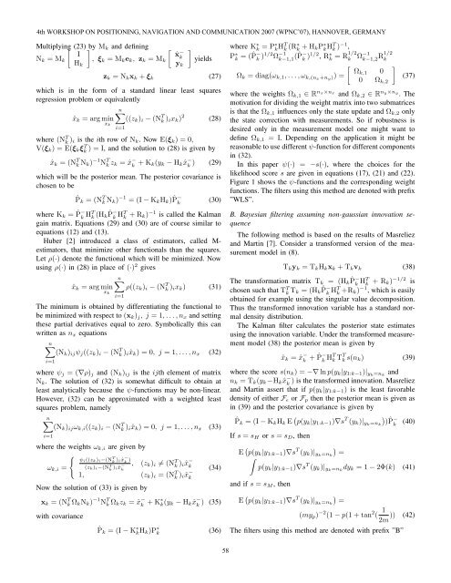
Multiply<strong>in</strong>g (23) by<br />
Mk and def<strong>in</strong><strong>in</strong>g<br />
I<br />
Nk =Mk , ξk =Mkek, zk =Mk<br />
Hk<br />
zk =Nkxk + ξk<br />
ˆx −<br />
k<br />
yk<br />
<br />
yields<br />
(27)<br />
which is <strong>in</strong> the form of a standard l<strong>in</strong>ear least squares<br />
regression problem or equivalently<br />
n<br />
ˆxk =argm<strong>in</strong> ((zk)i − (N<br />
xk<br />
T k )ixk) 2<br />
(28)<br />
i=1<br />
where (NT k )i is the ith row of Nk. NowE(ξk) =0,<br />
V(ξk) =E(ξkξT k )=I, and the solution to (28) is given by<br />
ˆxk =(N T k Nk) −1 N T k zk =ˆx −<br />
k +Kk(yk − Hk ˆx −<br />
k<br />
) (29)<br />
which will be the posterior mean. The posterior covariance is<br />
chosen to be<br />
ˆPk =(N T k Nk) −1 =(I− KkHk) ˆ P −<br />
k<br />
(30)<br />
where Kk = ˆ P −<br />
k HT k (Hk ˆ P −<br />
k HT k +Rk) −1 is called the <strong>Kalman</strong><br />
ga<strong>in</strong> matrix. Equations (29) and (30) are of course similar to<br />
equations (12) and (13).<br />
Huber [2] <strong>in</strong>troduced a class of estimators, called Mestimators,<br />
that m<strong>in</strong>imize other functionals than the squares.<br />
Let ρ(·) denote the functional which will be m<strong>in</strong>imized. Now<br />
us<strong>in</strong>g ρ(·) <strong>in</strong> (28) <strong>in</strong> place of (·) 2 gives<br />
n<br />
ˆxk =argm<strong>in</strong> ρ((zk)i − (N<br />
xk<br />
T k )ixk) (31)<br />
i=1<br />
The m<strong>in</strong>imum is obta<strong>in</strong>ed by differentiat<strong>in</strong>g the functional to<br />
be m<strong>in</strong>imized with respect to (xk)j, j=1,...,nx and sett<strong>in</strong>g<br />
these partial derivatives equal to zero. Symbolically this can<br />
written as nx equations<br />
n<br />
(Nk)ijψj((zk)i − (N T k )iˆxk) =0, j =1,...,nx (32)<br />
i=1<br />
where ψj =(∇ρ)j and (Nk)ij is the ijth element of matrix<br />
Nk. The solution of (32) is somewhat difficult to obta<strong>in</strong> at<br />
least analytically because the ψ-functions may be non-l<strong>in</strong>ear.<br />
However, (32) can be approximated with a weighted least<br />
squares problem, namely<br />
n<br />
(Nk)ijωk,i((zk)i − (N T k )iˆxk) =0, j =1,...,nx (33)<br />
i=1<br />
where the weights ωk,i are given by<br />
<br />
ψi((zk)i−(N<br />
ωk,i =<br />
T<br />
k<br />
)i ˆx− k )<br />
(zk)i−(NT k<br />
)i ˆx− k<br />
, (zk)i = (NT −<br />
k )iˆx k<br />
1, (zk)i =(NT k<br />
Now the solution of (33) is given by<br />
)iˆx −<br />
k<br />
xk =(N T k ΩkNk) −1 N T k Ωkzk =ˆx −<br />
k +K∗k(yk − Hk ˆx −<br />
k<br />
with covariance<br />
ˆPk =(I− K ∗ kHk)P ∗ k<br />
(34)<br />
) (35)<br />
(36)<br />
58<br />
where K∗ k =P∗ kHT k (R∗ k +HkP∗ kHT k )−1 ,<br />
P∗ k =(ˆ P −<br />
k )1/2Ω −1<br />
k−1,1 (ˆ P −<br />
k )1/2 , R∗ k =R1/2<br />
k Ω−1<br />
k−1,2R1/2 k<br />
<br />
Ωk,1 0<br />
Ωk =diag(ωk,1,...,ωk,(nx+ny)) =<br />
0 Ωk,2<br />
<br />
(37)<br />
where the weights Ωk,1 ∈ R nx×nx and Ωk,2 ∈ R ny×ny . The<br />
motivation for divid<strong>in</strong>g the weight matrix <strong>in</strong>to two submatrices<br />
is that the Ωk,1 <strong>in</strong>fluences only the state update and Ωk,2 only<br />
the state correction with measurements. So if robustness is<br />
desired only <strong>in</strong> the measurement model one might want to<br />
def<strong>in</strong>e Ωk,1 =I. Depend<strong>in</strong>g on the application it might be<br />
reasonable to use different ψ-function for different components<br />
<strong>in</strong> (32).<br />
In this paper ψ(·) = −s(·), where the choices for the<br />
likelihood score s are given <strong>in</strong> equations (17), (21) and (22).<br />
Figure 1 shows the ψ-functions and the correspond<strong>in</strong>g weight<br />
functions. The filters us<strong>in</strong>g this method are denoted with prefix<br />
”WLS”.<br />
B. Bayesian filter<strong>in</strong>g assum<strong>in</strong>g non-gaussian <strong>in</strong>novation sequence<br />
The follow<strong>in</strong>g method is based on the results of Masreliez<br />
and Mart<strong>in</strong> [7]. Consider a transformed version of the measurement<br />
model <strong>in</strong> (8).<br />
Tkyk =TkHkxk +Tkvk<br />
(38)<br />
The transformation matrix Tk = (Hk ˆ P −<br />
k HT k +Rk) −1/2 is<br />
chosen such that TT k Tk =(Hk ˆ P −<br />
k HT k +Rk) −1 , which is easily<br />
obta<strong>in</strong>ed for example us<strong>in</strong>g the s<strong>in</strong>gular value decomposition.<br />
Thus the transformed <strong>in</strong>novation variable has a standard normal<br />
density distribution.<br />
The <strong>Kalman</strong> filter calculates the posterior state estimates<br />
us<strong>in</strong>g the <strong>in</strong>novation variable. Under the transformed measurement<br />
model (38) the posterior mean is given by<br />
ˆxk =ˆx −<br />
k + ˆ P −<br />
k HT k T T k s(nk) (39)<br />
where the score s(nk) =−∇ ln p(yk|y1:k−1)|yk=nk and<br />
nk =Tk(yk−Hk ˆx −<br />
) is the transformed <strong>in</strong>novation. Masreliez<br />
k<br />
and Mart<strong>in</strong> assert that if p(yk|y1:k−1) is the least favorable<br />
density of either Fɛ or Fp then the posterior mean is given as<br />
<strong>in</strong> (39) and the posterior covariance is given by<br />
ˆPk =(I−KkHk E p(yk|y1:k−1)∇s T <br />
(yk)|yk=nk ) Pˆ −<br />
k (40)<br />
If s = sH or s = sD, then<br />
E p(yk|y1:k−1)∇s T <br />
(yk)|yk=nk =<br />
<br />
p(yk|y1:k−1)∇s T (yk)|yk=nk dyk =1− 2Φ(k) (41)<br />
and if s = sM , then<br />
E p(yk|y1:k−1)∇s T <br />
(yk)|yk=nk =<br />
(myp) −2 (1 − p(1 + tan 2 ( 1<br />
)) (42)<br />
2m<br />
The filters us<strong>in</strong>g this method are denoted with prefix ”B”


