Local Government Fund Presentation - Ohio Department of Taxation

- A History of the Local Government Fund 

and the Local Government Revenue 

Assistance Fund - 

By Christopher Hall, Ohio Department of Taxation 

Presented to the Local Government and Library Revenue 

Distribution Task Force 

January 31, 2006

Presentation Organization 

• Introductory discussion of general purpose “revenue 

sharing” and basic description of the LGF and LGRAF 

• Origins of the LGF and changes made through the 1980’s 

• Discussion of the LGRAF 

• LGF and LGRAF developments since the early 1990’s 

• Final comments and observations

Structure of the LGF, Part One: 

Monthly distributions to 88 county undivided 

local government funds 

Adams County Undivided LGF 

(may also receive dealer in intangibles revenue) 

Distributions to subdivisions: 

County Govt. 

Townships 

Municipalities 

State Local Government Fund 

(Funded by major state taxes) 

Approx. 91% of State LGF goes to 88 county undivided LGFs 

86 other undivided LGFs 


Distributions to subdivisons: 

County Govt. 

Townships 


Park Districts (34 counties) 

Wyandot County Undivided LGF 


Distributions to subdivisions 

County Govt. 

Townships 

Municipalities

Structure of the LGF, Part Two: 

Monthly distributions to municipalities with 

an income tax 

State Local Government Fund 

(Funded by major state taxes) 

Approx. 9% of State LGF goes to 541 municipalities with an income tax 

Village of Manchester (Adams Co.) 539 other municipalities Village of Sycamore (Wyandot Co.)

Summary of LGF/LGRAF Estimation & 

Distribution Process 

• By July 15, Tax Commissioner certifies to each county auditor the 

estimated amount to be distributed to the county undivided LGF and 

the county undivided LGRAF during the following calendar year 

• In August, the county budget commission computes each subdivision’s 

share of the county undivided LGF and LGRAF for the next calendar 

year; within 10 days, county auditor reports those amounts to the 

subdivisions 

• Each month the Tax Commissioner distributes the prior month’s LGF 

(and dealer in intangibles taxes) deposits and LGRAF deposits to each 

county undivided LGF and LGRAF, respectively, using each county’s 

percentage share computed in the preceding July; a portion of the LGF 

is also distributed monthly to municipalities with an income tax; 

distributions are made by the 10 th of each month 

• County treasurer distributes the amount received in the undivided LGF 

and undivided LGRAF to the various subdivisions based on 

subdivision percentage shares authorized by the county budget 

commission

General Purpose Revenue Sharing 

• The LGF and LGRAF, along with the Library and Local 

Government Support Fund (LLGSF), comprise the state’s 

“general purpose revenue sharing” programs for local 

governments 

• Ohio has other revenue sharing programs – e.g., sharing of 

motor fuel tax and of estate tax revenues – but they do not 

constitute “general purpose” revenue sharing 

• The LGF, LGRAF and LLGSF have two key 

characteristics not simultaneously present with other 

revenue sharing programs: 

– The money is not for specific purposes (for the general fund) 

– The money goes to local governments based on criteria other than 

the origin of the tax revenues

General Purpose Revenue Sharing (con’d) 

• The federal government had a general revenue sharing 

program which originated during the Nixon Administration 

• A portion of federal revenues was shared with states and 

local governments 

• Revenue sharing was a product of that administration’s 

“New Federalism”, providing revenues to states and local 

governments with few programmatic requirements (in 

contrast to the many categorical grant programs developed 

during the 1960’s) 

• Federal revenue sharing with local governments existed 

from 1972 to 1986 (although revenue sharing with states 

ended after 1981), terminated as a result of deficit 

reduction.

Origins of General Revenue Sharing in Ohio 

• Ohio’s general purpose revenue sharing program 

originated well before the federal program 

• The Local Government Fund was created when the state 

sales tax was enacted in December 1934 

• Revenue from the new 3% state sales tax was to be used 

for a county poor relief excise fund and for a state public 

school fund, with any remaining revenue to be used for the 

new “Local Government Fund” 

• In the first year of the LGF (1935), $10.7 million was sent 

to local governments, out of $45.1 million in total state 

sales tax revenue


(con’d) 

• Basic structure of the original LGF has been maintained to 

this day: state revenue earmarked for LGF (replaced by an 

appropriation beginning in 1939); LGF monies distributed 

to 88 undivided LGFs; and funds subsequently distributed 

by county budget commission to eligible subdivisions 

• Between 1935 and 1938 the portion of the state sales tax 

directed to the LGF varied, with the percentage during that 

period varying between 24% and 32% 

• Beginning in 1939, the earmarking concept was replaced 

by annual appropriations (i.e., a flat $12 million annual 

appropriation through 1944, with increases during the 

1945-1947 period)


(con’d) 

• Originally, the State LGF was distributed to 88 county 

undivided LGFs based on each county’s proportionate 

share of municipal valuation (real, tangible personal and 

utility property); the average valuation over the preceding 

five years was used 

• Distribution effect: The higher a county’s municipal 

valuation, the higher its LGF distribution 

• Starting in 1945 (when the LGF was increased from $12 to 

$16 million), 75% of the LGF was distributed based on 

each county’s share of municipal valuation and 25% was 

distributed based on each county’s share of population 

• The valuation-population distribution criteria, as well as 

the relative 75% -25% weights, exist to this day


(con’d) 

• Subdivisions receiving county undivided LGF monies: 

counties, municipal corporations, park districts, and 

townships 

• From the beginning, state law has required monies from 

each county undivided LGF to be apportioned to the 

county’s subdivisions based on the relative “need” of each 

subdivision 

• According to the original statute, the county budget 

commission convenes to consider facts and information 

presented by the county auditor and then determine the 

amount needed by the subdivision for its current operating 

expenses (to the extent those expenses exceed revenues 

available from all other sources)


(con’d) 

• The concept of subdivision “need” developed over time 

into a contentious and complex exercise resulting in 

considerable litigation, new case law, and occasional 

statutory revisions 

• This presentation shall not dwell extensively on how funds 

are apportioned to subdivisions, in part due to the state’s 

traditionally limited role in this process and also due to the 

need to focus primarily on the state’s funding for and 

allocation to the 88 county undivided funds 

• However, a basic description of the subdivision 

apportionment process will be provided later in the 

presentation

Post-War LGF Developments 

• In 1947, the five-year measurement for municipal 

valuation was replaced by a single-year measurement 

(using the second year next preceding the year of 

distribution); this arrangement exists to this day 

• Significant LGF changes occurred in the 1940’s, at a time 

of post-WWII local government fiscal crises (revenue 

streams inadequate to meet rapidly rising costs) 

• Major LGF funding increases during 1945-1947 period 

• Department of Taxation issued a 1947 study of the Ohio 

state and local government revenue system 

• In response to one study recommendation, the General 

Assembly converted three state-collected intangibles taxes 

from being a state revenue source to being a local 

government revenue source

Post-War LGF Developments (con’d) 

• The three converted intangibles taxes were: 2-mill tax paid 

by financial institutions on their deposits; 2-mill tax on the 

shares and capital of financial institutions; and 5-mill tax 

on the shares and capital of dealers in intangibles 

• County undivided LGFs received monies from both these 

state-collected intangibles taxes and the state LGF 

• The three intangibles taxes together generated $15 million 

for local governments in 1948 

• These revenues were distributed to the counties of origin 

(physical location of deposits, etc.) 

• The LGF allocation was reduced to $12.0 million in 1948 

(from $27.3 million in 1947); combined 1948 intangibles 

and LGF revenues nearly the same as 1947 LGF revenues

Post-War LGF Developments (con’d) 

• Cutting the LGF, while simultaneously adding new originbased 

intangibles taxes, undoubtedly had distributional 

impacts (increases and decreases) across the counties 

• By the mid-1950’s, the intangibles tax comprised a 

majority of the combined LGF and intangibles tax 

distributions 

• There was growth in intangibles taxes while the 

appropriated LGF grew little in the 1950’s and 1960’s (no 

LGF growth between 1958 and 1969) 

• The intangibles tax share peaked in 1969, when it 

comprised 68% of the total ($51 million intangibles tax vs. 

$24 million LGF) 

• There were few other LGF changes during the 1950’s and 

1960’s worth noting

Apportionment of County Undivided LGF to 

Subdivisions 

• With the enactment of SB 114 in 1969, most of the 

existing law pertaining to subdivision apportionment was 

put into place 

• SB 114 dealt with a variety of problems related to how 

subdivision “needs” are computed 

• In current RC 5747.51 and .52, a process is prescribed for 

how budget commissions are to use subdivision tax budget 

information to derive each subdivision’s relative “need”, 

subsequently translated into a percentage share of the 

county’s total undivided LGF 

• This process is generally termed the “statutory” method of 

apportionment 

• The most important long-term change in SB 114 was the 

enactment of an “alternative” method of apportionment


Subdivisions (con’d) 

• The “statutory” method of subdivision apportionment 

resulted in considerable contention and litigation 

• In contrast, the “alternative” approach allows a county to 

derive a specific distribution formula for that particular 

county, thus avoiding many of the problems associated 

with the “statutory” formula (such as tax budgets 

developed to exaggerate needs) 

• 80 of the 88 counties have adopted an “alternative” 

formula 

• In order to adopt or change an “alternative” formula, the 

county budget commission develops the new or changed 

formula and following parties must assent to that formula: 

board of county commissioners; the most populous city in 

the county; and a majority of the townships and 

municipalities located in the county


Subdivisions (con’d) 

• Despite the wide discretion allowed in crafting an 

“alternative” apportionment formula, there are several 

substantive restrictions contained in the statute 

• The county as a subdivision may receive no more than an 

established percentage of the total undivided fund, based 

on the percentage of the county’s population located within 

a municipal corporation: (1) Municipal population is less 

than 41% -- maximum county share is 60%; (2) 41%-80% 

municipal population -- 50% maximum county share; (3) 

81% or larger municipal population – 30% maximum 

county share 

• If a county’s population is under 100,000 no less than 10% 

of the undivided LGF is to be distributed to townships

LGF Developments in the 1970’s 

• Major changes to the LGF took place in 1972, in the wake 

of the recently enacted state income tax 

• In calendar year 1972, $48 million of state income tax 

money was earmarked for the LGF, a 17% increase over 

1971 

• At the same time, 1/12 th of the LGF was now dedicated to 

municipalities imposing an income tax, in recognition that 

the state’s imposition of an income tax would make it more 

difficult for municipalities to obtain voter approval for 

rates exceeding 1%

LGF Developments in the 1970’s (con’d) 

• In calendar year 1973, the fixed-dollar LGF allocations 

were replaced by a bona fide revenue sharing concept 

• 3.5% of the state income tax, sales tax and corporate 

franchise tax were now dedicated to the LGF 

• Local governments benefited from near-record growth in 

combined intangibles tax and LGF distributions during the 

1970’s 

• However, much of this growth was mitigated by high 

inflation (particularly during the late 1970’s) 

• Minimum annual county undivided LGF distribution 

revised in 1973, becoming $150,000; in 1975, 37 counties 

were at the $150,000 minimum

LGF Developments in the 1980’s 

• The severe economic recession of the early 1980’s resulted 

in a state fiscal crisis 

• Major tax and revenue changes occurred, and there were 

substantial revisions to the LGF and intangibles taxes 

• HB 694 (FY 1982-83 budget bill) eliminated the tax on 

financial institution shares and capital beginning in CY 

1982; such companies were made subject to corporate 

franchise tax 

• The bill also phased out the 2-mill tax on financial 

institution deposits: 1.375 mills in CY 1982 and CY 1983, 

and no deposits tax thereafter 

• Without a revenue replacement, these changes would 

dramatically reduce distributions to local governments


• The portion of the corporate franchise tax earmarked for 

the LGF was increased in order to make up for the reduced 

intangibles tax distributions 

• In CY 1982, 3.5% of franchise tax was earmarked for State 

LGF and 7.75% of the franchise tax was distributed to 

counties based on their share of 1981 intangibles tax 

revenues 

• Minimum LGF distribution increased to $225,000 

• State sales tax rate increased by 1% (to 5%), with a 

requirement that none of the increased sales tax revenue in 

FY 1982 and 1983 would go to the LGF; percentage 

contribution to LGF from the sales tax was reduced 

accordingly


• Similarly, a temporary income tax increase was enacted in 

1982 (SB 530, 114 th GA) with a provision that none of the 

increased revenue was to go to the LGF; this provision was 

eliminated when the income tax increase was made 

permanent in 1983 (HB 100, 115 th GA) 

• Additional major changes were enacted during the FY 

1984-1985 budget cycle 

• HB 291 (FY 1984-85 budget bill) repealed the special 

contribution schedule for the franchise tax; instead, 14.5% 

of the franchise tax was dedicated to the LGF with no 

special allocations to counties based on historical 

intangibles tax distributions 

• This new formula caused major distributional shifts among 

the counties


• When it became apparent that an estimated 50 counties 

would lose money in 1984 compared to 1983 and 38 

counties would gain money, another bill was passed (SB 

293, eff. December 1, 1983) to resolve that situation 

• The SB 293 changes to the distribution formula are 

essentially reflected in the statute as it exists today (see 

next two pages); only difference is that county undivided 

LGFs now receive 90% (less $6 million) of the LGF, while 

prior law provided 11/12ths (less $6 million) 

• SB 293 increased the fund by changing the corporate 

franchise tax share from 14.5% to 15.4% 

• Dealer in intangibles tax is the only part of the intangibles 

tax still remaining; 5 mills of the tax is distributed to 

county LGFs based on location of dealers’ gross receipts

Current LGF Distribution Formula to the 88 

County Undivided LGF’s 

• Tax Commissioner computes amounts under two formulas 

• Formula One: Each county receives its 1983 deposits tax at 

a 2-mill rate; 90% of remaining fund (less $6 million) 

distributed using population (25%) and municipal 

valuation (75%), with minimum distribution of $225,000 

• Formula Two: 90% of the total LGF (less $6 million) is 

distributed to each county based on population (25%) and 

municipal valuation (75%); $225,000 min. distribution 

• The higher allocation is identified and assigned to each 

county, and those amounts added to reach a statewide total 

• Each county’s percentage share of the statewide assigned 

amounts is computed; this figure constitutes the county’s 

% share of the actual LGF deposits for the calendar year 

• Each county guaranteed to receive its 1983 distribution

Hypothetical Calendar Year 2005 LGF Distribution to Fayette County Pursuant to the LGF Statute 

Assumes that "freeze"-based LGF funding levels are used instead of the funding levels resulting from the statutory "percentage of revenue" 

method. Thus, total distributions from the state LGF to the 88 county undivided local government funds are assumed to equal the $604 

million that were actually dispersed in CY 2005 pursuant to the "freeze". 

1. Compute "Formula One" and "Formula Two" distributions. 

"Formula One" distribution: RC 5747.501(A)(1) (a) (b) (a) x (b) 

Fayette Share Fayette Frequency with which the 

State Total of Total Amount shares are updated 

Amount distributed according to population $114,523,131 0.250% $286,814 Updated every 10 years 

Amount distributed according to municipal valuation 

Adjustment to ensure that each county receives a 

distribution of at least $225,000 from the two above 

combined formulas (a total of $52,406 is given to Noble and 

Vinton counties and proportionally taken from all other counties in 

343,569,394 0.176% 604,386 Updated annually 

order to meet this requir 

Amount distributed based on 145.45% of county's 1983 

0 n/a (80) n/a 

deposits tax receipts 145,971,478 0.208% 303,617 Not updated 

TOTAL $604,064,003 $1,194,737 

"Formula Two" distribution: RC 5747.501(A)(2) (a) (b) (a) x (b) 

State Total 

Fayette Share 

of Total 

Fayette 

Amount 

Frequency with which the 

shares are updated 

Amount distributed according to population $147,411,360 0.250% $369,180 Updated every 10 years 

Amount distributed according to municipal valuation 

Adjustment to ensure that each county receives a 

distribution of at least $225,000 from the two above 

combined formulas (no adjustment needed - all counties meet the 

442,234,079 0.176% 777,951 Updated annually 

$225,000 minimum) 0 n/a 0 n/a 

TOTAL $589,645,439 $1,147,130 

Note: The adjusted 1983 deposits tax is not a part of "formula two". 

2. Determine Fayette County's "assigned amount" and percentage share of total state LGF 

distribution. The assigned amount is the greater of the "formula one" or "formula two" distributions 

computed for each county. [RC 5747.501(B), (C)] 

Total "assigned amounts" for all counties $619,329,508 (a) 

Fayette County's "assigned amount" $1,194,737 (b) 

Fayette County's share of assigned amounts 0.193% (b)/(a) 

3. Derive Fayette County's estimated LGF distribution: RC 5747.51(A) 

Total estimated LGF distribution to all counties $604,064,003 (a) 

Fayette County's share of total LGF 0.193% (b) 

Fayette County's estimated LGF distribution $1,165,288 (a) x (b) 

Total distribution to county undivided LGFs from state LGF: 

Total LGF deposits (from the various contributing taxes) 

Less: 145.45% of 1983 deposits taxes ($146 million) 

Resulting difference is multiplied by 90% 

Plus: 145.45% of 1983 deposits taxes ($146 million) 

Less: $6 million 

Equals: Total distribution to county undivided LGFs from the LGF 

(Note: Remainder of the state LGF is distributed directly to municipalities with an income tax) 

This would have been Fayette County's share of statewide 

LGF distributions during CY 2005 if the statutory formula had 

not been replaced by the "freeze".

Creation of LGRAF, and other changes of the 

late 1980’s 

• In response to a legislative study of the LGF in the late 

1980’s, legislation was enacted in 1987 (HB 171, FY 

1988-89 budget bill) that added a new fund – the Local 

Government Revenue Assistance Fund - whose criteria for 

distribution had not yet been determined 

• HB 171 also increased the percentage earmarked for the 

LGF, increasing from 3.5% to 4.5% in February 1988 and 

then increasing to 4.6% in July 1989 

• Under HB 171, both the LGRAF and LGF would receive 

monies from two additional state revenue sources: the use 

tax and the public utility excise tax 

• Funding for the LGRAF began in July 1989, originally 

comprised of 0.3% of the same major tax sources that fund 

the LGF; this share was scheduled to increase to 0.6% in 

FY 1991, 0.65% in FY 1992, and 0.70% in FY 1993

Creation of LGRAF, and other changes of the 

late 1980’s (con’d) 

• HB 111 (the FY 1990-91 budget bill) stipulated that the 

LGRAF would be distributed based on each county’s share 

of total state population, using annually updated population 

figures (Census Bureau estimates for most years, and 

actual decennial Census population figures every 10 th year) 

• The LGRAF was patterned off the LGF in terms of 

distribution procedure and timing, and revenue sharing 

structure 

• Monies are distributed monthly from the State LGRAF to 

88 county undivided LGRAFs 

• Based on the subdivisions’ proportionate shares authorized 

by the county budget commission, the undivided LGRAF 

is distributed to the subdivisions by the 20 th of the month

Developments during the 1990s and beyond 

• Ohio experienced a recession in 1990-91 that required a 

variety of fiscal measures to balance the budget 

• As a state revenue saving device, HB 298 (the FY 1992-93 

budget bill) and HB 904 (budget balancing bill) 

temporarily suspended the LGF and LGRAF funding 

percentages from January 1992 through July 1993, 

constituting a “freeze” on distributions 

• Under the “freeze”, additional revenues that normally 

would have been deposited into the local funds are instead 

deposited into the state GRF (revenue growth in the 

contributing tax sources must occur in order for the GRF to 

realize this benefit)


(con’d) 

• For CY 1992, the total amount distributed from the LGF 

and LGRAF equaled the amounts distributed during 1991; 

during the January-July 1993 period, the total amount 

distributed equaled the January-July 1992 distributions 

• Although the “freeze” was lifted beginning in FY 1994, the 

respective LGF and LGRAF funding percentages were 

reduced to 4.2% (from 4.6%) and 0.6% (from 0.65%) 

• Since revenues were swiftly recovering, the reduced 

funding percentages resulted in moderate growth for the 

two funds while preventing a windfall and providing longterm 

savings for the state


(con’d) 

• SB 3, the electric deregulation bill, enacted a kilowatt hour 

tax on electric utilities to begin in June 2001 

• Electric utilities were also made subject to the corporate 

franchise tax but no longer made subject to the utility 

excise tax 

• A portion of revenues from the kilowatt hour tax was 

earmarked for the LGF (2.464%) and the LGRAF 

(0.378%) 

• The LGF and LGRAF contribution levels were the 

equivalent of 4.2% and 0.6%, respectively, of the kilowatt 

hour tax collections remaining after the amounts are 

credited to the local government and school district 

property tax replacement funds


(con’d) 

• HB 94 (FY 2002-03 budget) enacted a “freeze” in which 

each county undivided LGF (as well as each municipality 

receiving a direct LGF distribution) and each county 

undivided LGRAF would receive the same amount that it 

received in FY 2001 (July 2000-June 2001) 

• Revenue performance was so poor for most of the FY 

2002-03 biennium that the freeze essentially did not save 

the state GRF any revenue (in fact, a semi-annual 

reconciliation adjustment prevented a revenue loss); the 

only appreciable savings in the biennium came from a $30 

million reduction in 2003 enacted by HB 40 

• The freeze was extended into FY 2004-05 by HB 95


(con’d) 

• During FY 2004 and 2005, each recipient received the same amount it 

received in FY 2003 

• The state saved $127 million during FY 2004 and $241 million in FY 

2005 as a result of the freeze on all three funds (savings attributable to 

LGF and LGRAF were $100 million in FY 2004 and $162 million in 

FY 2005) 

• Note that the dealer in intangibles tax distributions were not affected 

by the freeze 

• The current biennial budget (HB 66) originally contained LGF and 

LGRAF cuts but ultimately extended the freeze for another two fiscal 

years 

• According to ODT estimates, the state will save $228 million in FY 

2006 and $252 million in FY 2007 (LGF and LGRAF savings= $145 

million in FY 2006 and $161 million in FY 2007)

Final Comments and Observations 

• See page 36 for a history of the LGF-intangibles tax 

allocations and the LGRAF allocations 

• Throughout much of its history (1948-1972), the LGF was 

appropriated and not based on a percentage of tax revenues 

• During the years when the LGF was an appropriated item, 

there was a complementary and modestly growing revenue 

source for CULGFs – the intangibles tax (now repealed 

except for the dealer in intangibles portion) 

• Since the 1980’s, the LGF and intangibles tax have ranged 

between 3% and 4% of the GRF 

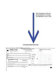
• There has been significant real (inflation-adjusted) growth 

in the LGF over the years, as shown on page 37

Final Comments and Observations (con’d) 

• If/when the freeze is discontinued, attention will need to be 

paid to the distribution formula to prevent wide 

distributional swings (positive and negative) on recipients 

• Since 2001, the formula has not been in effect, thereby 

insulating counties from the effects of valuation changes 

• The intangibles tax was repealed over 20 years ago but is 

still a part of the LGF formula 

• As a county’s urban property wealth rises relative to other 

counties, its share of the LGF increases 

• On a per capita basis, the LGF distributions to 88 county 

undivided LGFs ranges between $18 and $84; thus, the top 

county’s distribution is nearly five times as high as the 

lowest county 

• Because it is so complicated, the LGF formula is generally 

not understood and thus is not transparent

Calendar 

Year 1 

Local Government Fund and Intangibles Tax Allocations, Calendar Years 1935-2005 

(Figures are in millions of $) 

Local 

Government 

Yr-to-yr 

percentage 

change 

Local 

Government 

Fund 

Yr-to-yr 

percentage 

change 

Intangibles 

Calendar 

Fund Tax Total 

Year 1 

Intangibles 

Tax Total 

1935 $10.7 $0.0 $10.7 -- 1971 $36.0 $56.8 $92.8 4.4% 

1936 17.9 0.0 17.9 67.3% 1972 42.0 61.6 103.6 11.5% 

1937 15.1 0.0 15.1 -15.6% 1973 53.3 68.1 121.4 17.2% 

1938 10.9 0.0 10.9 -27.6% 1974 55.2 75.8 131.0 7.9% 

1939 12.0 0.0 12.0 9.6% 1975 59.9 82.7 142.6 8.9% 

1940 12.0 0.0 12.0 0.0% 1976 63.8 88.9 152.7 7.1% 

1941 12.0 0.0 12.0 0.0% 1977 74.1 97.8 171.9 12.6% 

1942 12.0 0.0 12.0 0.0% 1978 87.3 108.2 195.5 13.7% 

1943 12.0 0.0 12.0 0.0% 1979 96.4 119.5 215.9 10.4% 

1944 12.0 0.0 12.0 0.0% 1980 102.8 129.4 232.1 7.5% 

1945 16.0 0.0 16.0 33.3% 1981 105.9 135.3 241.2 3.9% 

1946 21.0 0.0 21.0 31.3% 1982 161.4 99.5 260.9 8.2% 

1947 27.3 0.0 27.3 29.8% 1983 165.9 104.5 270.5 3.7% 

1948 12.0 15.1 27.1 -0.6% 1984 277.4 4.8 282.2 4.3% 

1949 2 

6.0 0.0 6.0 -- 1985 298.4 6.0 304.5 7.9% 

1950 18.0 15.4 33.4 -- 1986 313.9 6.7 320.6 5.3% 

1951 18.0 15.8 33.8 1.1% 1987 337.7 7.7 345.4 7.7% 

1952 21.4 16.8 38.2 13.0% 1988 361.0 8.3 369.3 6.9% 

1953 18.0 17.5 35.5 -7.2% 1989 361.0 7.7 368.7 -0.2% 

1954 20.0 18.7 38.7 9.2% 1990 425.3 4.8 430.1 16.7% 

1955 20.0 21.6 41.6 7.5% 1991 425.7 7.2 432.9 0.7% 

1956 22.0 21.4 43.5 4.3% 1992 425.7 7.0 432.7 -0.1% 

1957 22.0 23.4 45.4 4.4% 1993 445.8 8.0 453.8 4.9% 

1958 24.0 24.8 48.8 7.5% 1994 478.1 8.5 486.6 7.2% 

1959 24.0 26.2 50.2 2.9% 1995 527.6 9.6 537.2 10.4% 

1960 24.0 27.3 51.3 2.3% 1996 543.9 9.6 553.4 3.0% 

1961 24.0 28.8 52.8 2.8% 1997 579.9 11.0 590.9 6.8% 

1962 24.0 30.3 54.3 2.9% 1998 632.5 10.0 642.5 8.7% 

1963 24.0 32.7 56.7 4.4% 1999 664.8 10.7 675.5 5.1% 

1964 24.0 34.8 58.8 3.7% 2000 692.2 13.9 706.1 4.5% 

1965 24.0 37.4 61.4 4.4% 2001 705.4 15.9 721.3 2.2% 

1966 24.0 40.3 64.3 4.8% 2002 670.3 11.2 681.5 -5.5% 

1967 24.0 43.7 67.7 5.2% 2003 662.2 9.1 671.3 -1.5% 

1968 24.0 46.7 70.7 4.5% 2004 662.2 10.4 672.6 0.2% 

1969 24.0 51.0 75.0 6.1% 2005 662.2 11.3 673.5 0.1% 

1970 34.0 54.9 88.9 18.5% 

1 

1950-1981 figures are based on fiscal years. 

2 

Six-month period; state converted to July-June fiscal year in July 1949. 

Local Government Revenue Assistance Fund Allocations, Calendar Years 1989-2005 

(Figures are in millions of $) 

Calendar 

Year 3 

Total 

Yr-to-yr 

percentage 

change 

Calendar 

Year 3 

Total 

Yr-to-yr 

percentage 

change 

1989 $12.9 -- 1998 $90.4 9.1% 

1990 38.1 194.8% 1999 95.0 5.1% 

1991 57.3 50.3% 2000 99.0 4.1% 

1992 57.3 0.0% 2001 100.8 1.8% 

1993 59.3 3.4% 2002 95.8 -4.9% 

1994 68.4 15.4% 2003 94.6 -1.3% 

1995 72.9 6.7% 2004 94.6 0.0% 

1996 77.8 6.7% 2005 94.6 0.0% 

1997 82.9 6.5% 

3 Fund began on July 1, 1989.

$900,000 

$800,000 

$700,000 

$600,000 

$500,000 

$400,000 

$300,000 

$200,000 

$100,000 

$0 

Total State Local Government Fund and Intangibles Tax 

Distributions, 1935 - 2005 

Showing both nominal and inflation-adjusted dollars 

1950-1980 figures are fiscal years; other figures are calendar years 

(Thousands of Dollars) 

1935 1940 1945 1950 1955 1960 1965 1970 1975 1980 1985 1990 1995 2000 2005 

Real (2005) Dollars Nominal Dollars

CALENDAR YEAR 2005 ACTUAL AND HYPOTHETICAL (STATUTORY) AMOUNTS 

DISTRIBUTED TO COUNTY UNDIVIDED LOCAL GOVERNMENT FUNDS 

(excludes dealer in intangibles tax distributions) 

Column identification 

(a) (b) (c) (c)/(a)=(d) (e) (f) (f)/(a)=(g) (h) (d)-(g)=(i) 

Actual Hypothetical Actual 

Actual per capita LGF Per capita LGF per capita per capita 

July 2004 Percent of Actual per capita distributions distributions if distributions distributions distributions 

estimated total estimated LGF LGF as % of mean statutory dist. if statutory as % of mean minus statutory 

Ohio county July 2004 distributions distributions per capita formula had formula had per capita per capita 

population population to counties to counties distribution been in effect* been in effect* distribution distributions** 

Adams 28,398 0.25% $644,701 $22.70 43.1% $648,866 $22.85 43.3% ($0.15) 

Allen 106,873 0.93% 4,413,326 41.30 78.3% 4,411,543 41.28 78.3% 0.02 

Ashland 54,058 0.47% 2,039,999 37.74 71.6% 2,024,322 37.45 71.0% 0.29 

Ashtabula 103,152 0.90% 3,826,555 37.10 70.4% 3,793,874 36.78 69.8% 0.32 

Athens 63,187 0.55% 1,873,300 29.65 56.2% 1,882,383 29.79 56.5% (0.14) 

Auglaize 46,938 0.41% 2,285,404 48.69 92.4% 2,225,865 47.42 90.0% 1.27 

Belmont 69,366 0.61% 2,722,412 39.25 74.5% 2,705,398 39.00 74.0% 0.25 

Brown 44,239 0.39% 964,547 21.80 41.4% 1,049,931 23.73 45.0% (1.93) 

Butler 346,560 3.02% 14,090,266 40.66 77.1% 14,518,452 41.89 79.5% (1.24) 

Carroll 29,576 0.26% 687,875 23.26 44.1% 697,105 23.57 44.7% (0.31) 

Champaign 39,645 0.35% 1,361,276 34.34 65.1% 1,348,900 34.02 64.5% 0.31 

Clark 142,613 1.24% 5,427,373 38.06 72.2% 5,208,165 36.52 69.3% 1.54 

Clermont 188,614 1.65% 3,596,503 19.07 36.2% 3,562,763 18.89 35.8% 0.18 

Clinton 42,280 0.37% 1,546,103 36.57 69.4% 1,593,088 37.68 71.5% (1.11) 

Columbiana 111,519 0.97% 3,867,478 34.68 65.8% 3,719,509 33.35 63.3% 1.33 

Coshocton 37,039 0.32% 1,372,061 37.04 70.3% 1,326,772 35.82 68.0% 1.22 

Crawford 45,961 0.40% 2,059,009 44.80 85.0% 2,090,232 45.48 86.3% (0.68) 

Cuyahoga 1,351,009 11.79% 113,832,857 84.26 159.8% 111,309,074 82.39 156.3% 1.87 

Darke 53,260 0.46% 2,320,911 43.58 82.7% 2,165,715 40.66 77.1% 2.91 

Defiance 39,038 0.34% 1,754,018 44.93 85.2% 1,730,992 44.34 84.1% 0.59 

Delaware 142,503 1.24% 4,821,904 33.84 64.2% 6,152,552 43.17 81.9% (9.34) 

Erie 78,992 0.69% 3,698,525 46.82 88.8% 3,870,817 49.00 93.0% (2.18) 

Fairfield 136,063 1.19% 4,770,303 35.06 66.5% 5,174,399 38.03 72.1% (2.97) 

Fayette 28,134 0.25% 1,103,922 39.24 74.4% 1,165,288 41.42 78.6% (2.18) 

Franklin 1,088,971 9.50% 77,672,719 71.33 135.3% 80,100,247 73.56 139.5% (2.23) 

Fulton 42,919 0.37% 1,955,530 45.56 86.4% 1,976,110 46.04 87.3% (0.48) 

Gallia 31,256 0.27% 843,906 27.00 51.2% 812,182 25.98 49.3% 1.01 

Geauga 94,602 0.83% 2,441,878 25.81 49.0% 2,523,997 26.68 50.6% (0.87) 

Greene 152,233 1.33% 8,228,030 54.05 102.5% 8,354,068 54.88 104.1% (0.83) 

Guernsey 41,304 0.36% 1,393,740 33.74 64.0% 1,420,091 34.38 65.2% (0.64) 

Hamilton 814,611 7.11% 52,568,804 64.53 122.4% 49,723,302 61.04 115.8% 3.49 

Hancock 73,602 0.64% 3,980,794 54.09 102.6% 3,723,623 50.59 96.0% 3.49 

Hardin 32,171 0.28% 1,149,108 35.72 67.8% 1,138,004 35.37 67.1% 0.35 

Harrison 15,938 0.14% 521,545 32.72 62.1% 500,664 31.41 59.6% 1.31 

Henry 29,382 0.26% 1,199,888 40.84 77.5% 1,162,468 39.56 75.1% 1.27 

Highland 42,610 0.37% 1,268,992 29.78 56.5% 1,341,941 31.49 59.7% (1.71) 

Hocking 28,838 0.25% 774,110 26.84 50.9% 777,538 26.96 51.1% (0.12) 

Holmes 41,273 0.36% 797,944 19.33 36.7% 828,759 20.08 38.1% (0.75)









Huron 60,404 0.53% 2,648,662 43.85 83.2% 2,659,539 44.03 83.5% (0.18) 

Jackson 33,411 0.29% 1,071,297 32.06 60.8% 1,068,082 31.97 60.6% 0.10 

Jefferson 71,420 0.62% 3,907,180 54.71 103.8% 3,330,913 46.64 88.5% 8.07 

Knox 57,785 0.50% 1,872,800 32.41 61.5% 1,904,025 32.95 62.5% (0.54) 

Lake 232,061 2.03% 17,844,978 76.90 145.9% 17,042,120 73.44 139.3% 3.46 

Lawrence 62,705 0.55% 1,657,141 26.43 50.1% 1,559,671 24.87 47.2% 1.55 

Licking 152,866 1.33% 6,530,772 42.72 81.0% 7,017,899 45.91 87.1% (3.19) 

Logan 46,616 0.41% 1,724,416 36.99 70.2% 1,724,535 36.99 70.2% (0.00) 

Lorain 294,324 2.57% 16,473,997 55.97 106.2% 17,553,377 59.64 113.1% (3.67) 

Lucas 450,632 3.93% 24,865,438 55.18 104.7% 25,286,173 56.11 106.4% (0.93) 

Madison 41,113 0.36% 1,334,677 32.46 61.6% 1,379,384 33.55 63.6% (1.09) 

Mahoning 249,755 2.18% 9,564,406 38.30 72.6% 9,147,650 36.63 69.5% 1.67 

Marion 66,310 0.58% 2,540,900 38.32 72.7% 2,530,948 38.17 72.4% 0.15 

Medina 165,077 1.44% 6,738,786 40.82 77.4% 7,334,079 44.43 84.3% (3.61) 

Meigs 23,286 0.20% 556,701 23.91 45.4% 527,606 22.66 43.0% 1.25 

Mercer 41,075 0.36% 1,827,279 44.49 84.4% 1,768,579 43.06 81.7% 1.43 

Miami 100,797 0.88% 5,158,759 51.18 97.1% 4,998,136 49.59 94.1% 1.59 

Monroe 15,063 0.13% 357,106 23.71 45.0% 333,927 22.17 42.1% 1.54 

Montgomery 550,063 4.80% 31,651,137 57.54 109.2% 30,496,094 55.44 105.2% 2.10 

Morgan 14,941 0.13% 366,792 24.55 46.6% 356,688 23.87 45.3% 0.68 

Morrow 34,247 0.30% 628,050 18.34 34.8% 680,874 19.88 37.7% (1.54) 

Muskingum 85,669 0.75% 2,852,403 33.30 63.2% 2,868,705 33.49 63.5% (0.19) 

Noble 14,021 0.12% 327,951 23.39 44.4% 341,596 24.36 46.2% (0.97) 

Ottawa 41,407 0.36% 1,602,885 38.71 73.4% 1,712,724 41.36 78.5% (2.65) 

Paulding 19,486 0.17% 620,111 31.82 60.4% 588,303 30.19 57.3% 1.63 

Perry 35,040 0.31% 801,414 22.87 43.4% 789,207 22.52 42.7% 0.35 

Pickaway 53,656 0.47% 1,691,418 31.52 59.8% 1,693,524 31.56 59.9% (0.04) 

Pike 28,294 0.25% 671,755 23.74 45.0% 691,465 24.44 46.4% (0.70) 

Portage 154,764 1.35% 6,017,002 38.88 73.8% 6,700,522 43.30 82.1% (4.42) 

Preble 42,553 0.37% 1,402,417 32.96 62.5% 1,401,061 32.93 62.5% 0.03 

Putnam 34,718 0.30% 1,401,561 40.37 76.6% 1,397,818 40.26 76.4% 0.11 

Richland 128,096 1.12% 6,034,072 47.11 89.4% 5,795,023 45.24 85.8% 1.87 

Ross 74,466 0.65% 2,688,332 36.10 68.5% 2,590,518 34.79 66.0% 1.31 

Sandusky 61,948 0.54% 2,821,855 45.55 86.4% 2,790,880 45.05 85.5% 0.50 

Scioto 77,046 0.67% 2,293,071 29.76 56.5% 2,174,968 28.23 53.6% 1.53 

Seneca 57,789 0.50% 2,684,243 46.45 88.1% 2,568,383 44.44 84.3% 2.00 

Shelby 48,517 0.42% 2,395,574 49.38 93.7% 2,309,150 47.59 90.3% 1.78 

Stark 381,229 3.33% 15,075,271 39.54 75.0% 15,342,920 40.25 76.3% (0.70) 

Summit 547,314 4.78% 35,230,987 64.37 122.1% 34,844,444 63.66 120.8% 0.71 

Trumbull 220,486 1.92% 8,716,062 39.53 75.0% 8,248,154 37.41 71.0% 2.12 

Tuscarawas 92,221 0.80% 4,280,984 46.42 88.1% 4,140,416 44.90 85.2% 1.52 

Union 44,487 0.39% 1,455,419 32.72 62.1% 1,735,331 39.01 74.0% (6.29) 

Van Wert 29,276 0.26% 1,278,300 43.66 82.8% 1,211,211 41.37 78.5% 2.29









Vinton 13,352 0.12% 290,735 21.77 41.3% 299,348 22.42 42.5% (0.65) 

Warren 189,276 1.65% 6,676,019 35.27 66.9% 8,847,518 46.74 88.7% (11.47) 

Washington 62,577 0.55% 2,205,751 35.25 66.9% 2,134,123 34.10 64.7% 1.14 

Wayne 113,577 0.99% 4,825,102 42.48 80.6% 4,708,870 41.46 78.6% 1.02 

Williams 38,912 0.34% 1,937,111 49.78 94.4% 1,821,834 46.82 88.8% 2.96 

Wood 123,278 1.08% 5,564,457 45.14 85.6% 5,812,335 47.15 89.4% (2.01) 

Wyandot 22,878 0.20% 1,022,853 44.71 84.8% 1,044,351 45.65 86.6% (0.94) 

TOTAL 11,459,011 100.00% $604,064,003 $52.72 100.0% $604,064,003 $52.72 100.0% $0.00 

*Assumes that the total amount distributed from the State LGF would remain "frozen" at $604,064,003 instead of being based on the "percentage of revenue" method. 

** If the statutory distribution method were restored, then the impact of that approach relative to the actual "freeze"-based distributions would be the inverse of amounts shown in this column 

(i.e., negative amounts become positive, and positive amounts become negative). 

Highest actual per capita distributions: Cuyahoga County 

Lowest actual per capita distributions: Morrow County 

Most favorable per capita treatment as a result of the freeze: Jefferson County 

Least favorable per capita treatment as a result of the freeze: Warren County

LOCAL GOVERNMENT REVENUE ASSISTANCE FUND: 

ACTUAL AND HYPOTHETICAL (STATUTORY) AMOUNTS DISTRIBUTED TO COUNTIES, CALENDAR YEAR 2005 

(a) (b) (c) (c)/(a)=(d) 


(e) (f) (f)/(a)=(g) (c)-(f)=(h) (i) 

County Per capita Actual 

Actual per capita LGRAF LGRAF per capita 

July 2003 Percent of Actual per capita distributions distributions if distributions if Actual distributions 

estimated total estimated LGRAF LGRAF as % of mean statutory dist. statutory dist. distributions minus statutory 

Ohio county July 2003 distributions distributions per capita formula had formula had minus statutory per capita 

population population to counties to counties distribution been in effect* been in effect* distributions** distributions** 

Adams 28,026 0.25% $241,201 $8.61 104.0% $231,833 $8.27 $9,369 $0.33 

Allen 108,241 0.95% 900,720 8.32 100.6% 895,376 8.27 5,344 0.05 

Ashland 53,749 0.47% 438,431 8.16 98.6% 444,615 8.27 (6,184) (0.12) 

Ashtabula 103,120 0.90% 869,817 8.43 102.0% 853,014 8.27 16,802 0.16 

Athens 64,380 0.56% 518,175 8.05 97.3% 532,555 8.27 (14,380) (0.22) 

Auglaize 46,740 0.41% 396,839 8.49 102.6% 386,636 8.27 10,203 0.22 

Belmont 69,636 0.61% 592,668 8.51 102.9% 576,033 8.27 16,635 0.24 

Brown 43,807 0.38% 347,295 7.93 95.8% 362,374 8.27 (15,079) (0.34) 

Butler 343,207 3.00% 2,796,776 8.15 98.5% 2,839,027 8.27 (42,251) (0.12) 

Carroll 29,599 0.26% 245,875 8.31 100.4% 244,845 8.27 1,030 0.03 

Champaign 39,544 0.35% 323,358 8.18 98.9% 327,110 8.27 (3,752) (0.09) 

Clark 143,351 1.25% 1,221,627 8.52 103.0% 1,185,807 8.27 35,819 0.25 

Clermont 185,799 1.62% 1,495,101 8.05 97.3% 1,536,940 8.27 (41,838) (0.23) 

Clinton 41,756 0.37% 340,133 8.15 98.5% 345,408 8.27 (5,275) (0.13) 

Columbiana 111,523 0.98% 937,708 8.41 101.6% 922,524 8.27 15,183 0.14 

Coshocton 37,132 0.32% 304,464 8.20 99.1% 307,158 8.27 (2,694) (0.07) 

Crawford 46,091 0.40% 396,454 8.60 104.0% 381,267 8.27 15,187 0.33 

Cuyahoga 1,363,888 11.93% 11,578,401 8.49 102.6% 11,282,157 8.27 296,244 0.22 

Darke 52,960 0.46% 455,517 8.60 104.0% 438,088 8.27 17,429 0.33 

Defiance 39,054 0.34% 334,387 8.56 103.5% 323,057 8.27 11,330 0.29 

Delaware 132,797 1.16% 833,142 6.27 75.8% 1,098,504 8.27 (265,362) (2.00) 

Erie 78,709 0.69% 657,052 8.35 100.9% 651,085 8.27 5,967 0.08 

Fairfield 132,549 1.16% 1,057,358 7.98 96.4% 1,096,453 8.27 (39,094) (0.29) 

Fayette 28,158 0.25% 239,393 8.50 102.8% 232,925 8.27 6,468 0.23 

Franklin 1,088,944 9.52% 8,629,478 7.92 95.8% 9,007,805 8.27 (378,327) (0.35) 

Fulton 42,446 0.37% 354,203 8.34 100.9% 351,116 8.27 3,087 0.07 

Gallia 31,398 0.27% 280,489 8.93 108.0% 259,726 8.27 20,763 0.66 

Geauga 93,941 0.82% 751,453 8.00 96.7% 777,085 8.27 (25,633) (0.27) 

Greene 151,257 1.32% 1,246,777 8.24 99.6% 1,251,206 8.27 (4,429) (0.03) 

Guernsey 41,362 0.36% 344,901 8.34 100.8% 342,149 8.27 2,753 0.07 

Hamilton 823,472 7.20% 7,099,061 8.62 104.2% 6,811,806 8.27 287,254 0.35 

Hancock 73,133 0.64% 582,575 7.97 96.3% 604,960 8.27 (22,386) (0.31) 

Hardin 31,608 0.28% 266,705 8.44 102.0% 261,463 8.27 5,242 0.17 

Harrison 15,967 0.14% 135,374 8.48 102.5% 132,080 8.27 3,294 0.21 

Henry 29,318 0.26% 251,634 8.58 103.8% 242,520 8.27 9,114 0.31 

Highland 41,963 0.37% 343,399 8.18 98.9% 347,120 8.27 (3,722) (0.09) 

Hocking 28,644 0.25% 244,985 8.55 103.4% 236,945 8.27 8,040 0.28 

Holmes 40,681 0.36% 320,805 7.89 95.3% 336,515 8.27 (15,710) (0.39) 

Huron 60,231 0.53% 508,649 8.44 102.1% 498,234 8.27 10,415 0.17

(a) (b) (c) (c)/(a)=(d) 


(e) (f) (f)/(a)=(g) (c)-(f)=(h) (i) 







Jackson 33,074 0.29% 274,603 8.30 100.4% 273,590 8.27 1,013 0.03 

Jefferson 71,888 0.63% 623,197 8.67 104.8% 594,662 8.27 28,536 0.40 

Knox 56,930 0.50% 451,712 7.93 95.9% 470,928 8.27 (19,216) (0.34) 

Lake 228,878 2.00% 1,900,513 8.30 100.4% 1,893,292 8.27 7,222 0.03 

Lawrence 62,550 0.55% 541,946 8.66 104.7% 517,417 8.27 24,529 0.39 

Licking 150,634 1.32% 1,150,376 7.64 92.3% 1,246,053 8.27 (95,676) (0.64) 

Logan 46,411 0.41% 391,990 8.45 102.1% 383,914 8.27 8,076 0.17 

Lorain 291,164 2.55% 2,374,939 8.16 98.6% 2,408,525 8.27 (33,586) (0.12) 

Lucas 454,216 3.97% 3,765,688 8.29 100.2% 3,757,300 8.27 8,388 0.02 

Madison 40,624 0.36% 348,863 8.59 103.8% 336,044 8.27 12,819 0.32 

Mahoning 251,660 2.20% 2,135,284 8.48 102.6% 2,081,745 8.27 53,539 0.21 

Marion 66,396 0.58% 555,679 8.37 101.2% 549,231 8.27 6,448 0.10 

Medina 161,641 1.41% 1,228,543 7.60 91.9% 1,337,103 8.27 (108,560) (0.67) 

Meigs 23,242 0.20% 202,117 8.70 105.1% 192,259 8.27 9,858 0.42 

Mercer 40,933 0.36% 345,914 8.45 102.2% 338,600 8.27 7,314 0.18 

Miami 100,230 0.88% 829,067 8.27 100.0% 829,108 8.27 (41) (0.00) 

Monroe 14,927 0.13% 129,759 8.69 105.1% 123,477 8.27 6,282 0.42 

Montgomery 552,187 4.83% 4,737,850 8.58 103.7% 4,567,722 8.27 170,128 0.31 

Morgan 14,843 0.13% 122,312 8.24 99.6% 122,782 8.27 (470) (0.03) 

Morrow 33,568 0.29% 268,264 7.99 96.6% 277,676 8.27 (9,412) (0.28) 

Muskingum 85,423 0.75% 712,781 8.34 100.9% 706,624 8.27 6,157 0.07 

Noble 14,054 0.12% 116,146 8.26 99.9% 116,255 8.27 (110) (0.01) 

Ottawa 41,192 0.36% 346,481 8.41 101.7% 340,743 8.27 5,738 0.14 

Paulding 19,665 0.17% 168,995 8.59 103.9% 162,670 8.27 6,325 0.32 

Perry 35,074 0.31% 288,516 8.23 99.4% 290,134 8.27 (1,618) (0.05) 

Pickaway 51,723 0.45% 450,829 8.72 105.4% 427,856 8.27 22,973 0.44 

Pike 28,194 0.25% 234,872 8.33 100.7% 233,222 8.27 1,650 0.06 

Portage 154,870 1.35% 1,274,786 8.23 99.5% 1,281,093 8.27 (6,307) (0.04) 

Preble 42,417 0.37% 365,105 8.61 104.1% 350,876 8.27 14,229 0.34 

Putnam 34,754 0.30% 296,540 8.53 103.1% 287,487 8.27 9,053 0.26 

Richland 128,267 1.12% 1,083,226 8.45 102.1% 1,061,032 8.27 22,195 0.17 

Ross 74,424 0.65% 636,626 8.55 103.4% 615,639 8.27 20,986 0.28 

Sandusky 61,753 0.54% 521,731 8.45 102.1% 510,824 8.27 10,907 0.18 

Scioto 77,453 0.68% 676,433 8.73 105.6% 640,696 8.27 35,738 0.46 

Seneca 57,734 0.50% 504,282 8.73 105.6% 477,579 8.27 26,703 0.46 

Shelby 48,566 0.42% 401,943 8.28 100.1% 401,741 8.27 202 0.00 

Stark 377,519 3.30% 3,141,233 8.32 100.6% 3,122,858 8.27 18,375 0.05 

Summit 546,773 4.78% 4,527,335 8.28 100.1% 4,522,937 8.27 4,398 0.01 

Trumbull 221,785 1.94% 1,896,001 8.55 103.3% 1,834,618 8.27 61,383 0.28 

Tuscarawas 91,706 0.80% 746,737 8.14 98.4% 758,597 8.27 (11,860) (0.13) 

Union 43,750 0.38% 338,829 7.74 93.6% 361,902 8.27 (23,074) (0.53) 

Van Wert 29,277 0.26% 253,693 8.67 104.8% 242,181 8.27 11,512 0.39 

Vinton 13,231 0.12% 103,360 7.81 94.4% 109,448 8.27 (6,087) (0.46)

(a) (b) (c) (c)/(a)=(d) 


(e) (f) (f)/(a)=(g) (c)-(f)=(h) (i) 







Warren 181,743 1.59% 1,265,349 6.96 84.2% 1,503,388 8.27 (238,039) (1.31) 

Washington 62,505 0.55% 531,917 8.51 102.9% 517,045 8.27 14,872 0.24 

Wayne 113,121 0.99% 931,617 8.24 99.6% 935,743 8.27 (4,126) (0.04) 

Williams 38,802 0.34% 318,679 8.21 99.3% 320,972 8.27 (2,293) (0.06) 

Wood 123,020 1.08% 1,009,896 8.21 99.2% 1,017,628 8.27 (7,733) (0.06) 

Wyandot 22,826 0.20% 192,625 8.44 102.0% 188,818 8.27 3,807 0.17 

TOTAL 11,435,798 100.00% $94,597,556 $8.27 100.0% $94,597,556 $8.27 $0 $0.00 

*Assumes that the total amount distributed from the LGRAF would remain "frozen" at $94,597,566 instead of being based on the "percentage of revenue" method. 

** If the statutory distribution method were restored, then the impact of that approach relative to the actual "freeze"-based distributions would be the inverse of amounts shown in these 

columns (i.e., negative amounts become positive, and positive amounts become negative). 

Highest actual per capita distributions: Gallia County 

Lowest actual per capita distributions: Delaware County 

Most favorable per capita treatment as a result of the freeze: Gallia County 

Least favorable per capita treatment as a result of the freeze: Delaware County

A. Local Government Fund and Dealer in Intangibles Tax Distributions by Type of Subdivision, CY 1999-2003 

Distribution from the 88 County Undivided LGFs (in millions) 

Calendar 

To Park 

To 

Direct 

Distribution 

from LGF to Total to 

Year To Counties To Townships Districts Municipalities Municipalities Municipalities Total 

1999 $222.3 $54.4 $11.0 $329.7 $57.4 $387.2 $674.9 

2000 232.3 57.2 11.7 343.2 61.1 404.4 705.6 

2001 237.1 58.4 12.1 349.9 62.4 412.3 719.9 

2002 224.8 55.6 11.4 331.6 59.0 390.6 682.4 

2003 222.1 55.6 11.2 324.9 58.1 383.0 671.8 

Calendar 

Each subdivision class as a percentage of total LGF distributions 


(including direct 

distribution from 

Year Counties Townships Park Districts 

LGF) Total 

1999 32.9% 8.1% 1.6% 57.4% 100.0% 

2000 32.9% 8.1% 1.7% 57.3% 100.0% 

2001 32.9% 8.1% 1.7% 57.3% 100.0% 

2002 32.9% 8.1% 1.7% 57.2% 100.0% 

2003 33.1% 8.3% 1.7% 57.0% 100.0% 

B. Local Government Revenue Assistance Fund Distributions by Type of Subdivision, CY 1999-2003 

Distribution from the 88 County Undivided LGRAFs (in millions) 

Calendar 

To Park 

To 

Year To Counties To Townships Districts Municipalities Total 

1999 $35.8 $11.0 $1.5 $46.7 $95.0 

2000 37.4 11.5 1.5 48.5 98.9 

2001 38.1 11.7 1.1 49.5 100.4 

2002 36.2 11.2 1.5 47.0 95.9 

2003 35.8 11.2 1.5 46.2 94.7 

Each subdivision class as a percentage of total LGRAF distributions 

Calendar 

Year Counties Townships Park Districts Municipalities Total 

1999 37.7% 11.5% 1.5% 49.2% 100.0% 

2000 37.8% 11.6% 1.6% 49.0% 100.0% 

2001 37.9% 11.7% 1.1% 49.3% 100.0% 

2002 37.7% 11.7% 1.6% 49.0% 100.0% 

2003 37.8% 11.8% 1.6% 48.8% 100.0%

Local Government Fund Presentation - Ohio Department of Taxation

Create successful ePaper yourself

Delete template?

Save as template?