Assessment of modeling approaches for the simulation of non ...

Assessment of modeling approaches for the simulation of non-premixed and partially
premixed turbulent combustion processes
Jan E. Anker, Kilian Claramunt, Charles Hirsch *
NUMECA International, Av. Franklin D. Roosevelt 5
B-1050 Brussels, Belgium
www.numeca.com
Abstract
This paper assesses two variants of the flamelet generated manifolds (FGM) technique as well as the Reaction-
Diffusion-Manifolds (REDIM) method for the simulation of non-premixed and partially premixed turbulent
combustion processes. For this purpose a framework for combustion models have been incorporated in the
unstructured, density-based Navier-Stokes solver FINE/Hexa. To be able to simulate combustion processes for low
Mach number flow, the implemented models are used in conjunction with a time-derivative preconditioning
technique. The FGM and the REDIM method are applied on a benchmark flame for purely non-premixed
combustion. The former method is also assessed on an industry-like test case, in which fuel and oxidizer partially
premix before combustion. A comparison of the results obtained with results using the classical flamelet method is
conducted to discuss the conceptual strengths and weaknesses of the different methods.
1. Introduction and objective of the paper
The mixture fraction modeling approach in conjunction
with flamelet tables [1] is recognized as a reliable and
accurate method for the simulation of diffusion flames.
As the flame-structure is calculated in a preprocessing
step and thus the chemistry calculations can be kept
outside of the flow solver, this method has the
advantage of being efficient. Due to the fast chemistry
assumption which is only partially relieved by
accounting for the effect of strain, this method is
however limited to the use for non-premixed flow.
There are several suggestions how to combine this
method with a Bray-Moss-Libby (BML) model for
premixed combustion to also be able to also simulate
partially premixed or even premixed combustion with
one single approach [2]. However, these models have
the drawback, that their performance, like the BML
model, depends on the adaption of the large set of
empirical coefficients to the particular application of
interest. A more fruitful approach in the development of
a reliable combustion model that both can handle nonpremixed
and premixed situations, seems to be to use a
manifold-based modeling technique, like the Flamelet
Generated Manifolds (FGM) method [3], the FPI
approach [4, 5], the ICE-PIC concept [6] or the
Reaction-Diffusion-Manifolds (REDIM) [7] method.
All these approaches employ tabulated chemistry in
conjunction with transport-equations for the mixture
fraction and one or several progress variables.
In this paper the FGM and the REDIM methods will
be assessed on a purely non-premixed test case as well
as a configuration with partially premixed combustion.
As a FGM either can be constructed from premixed or
non-premixed flamelets, it will be of interest to find out
which choice leads to the best performance of the
method. Vreman et al. [8] compared both methods on
TNF’s partially premixed Flame D [9]. As the fuel
• charles.hirsch@numeca.be
stream in Flame D is diluted with air, it is easy to
construct premixed flamelets for a large range of
fuel/oxidizer mixtures. In the current paper two different
test cases are chosen, for which burning premixed
flamelet solutions only exist on a limited range of the
mixture fraction. For both test cases the results obtained
by using a manifold-based method are compared to
those obtained with the classical flamelet method.
2. Modeling approaches
2.1 Governing equations
In the present approaches, the RANS-equations are
solved together with a transport equation for the mixture
fraction f and its variance g. A transport equation for the
progress variable Y is solved to parameterize the
evolution of the overall reaction. It is assumed that the
variance of the progress variable plays a negligible role
in the turbulence-chemistry interaction compared to the
variance of the mixture fraction.
The governing equations read as
t
t
~ r ( ρu
)
r
∂t
ρ + ∇ ⋅ = 0
~ r r ~ r ~ r
∂t
( ρu
) + ∇ ⋅ ( ρu
⊗ u −σ
) = 0
~ r
∂t
( ρf
) + ∇
( ρg~
r
∂ ) + ∇
∂
~ r~
r~
⋅ ( ρuf
− ρDe∇f
) = 0
~ r ( ρug~
r
ρDe
g~
r~
2
⋅ − ∇ ) = 2De
⋅ ( ∇f
) − Cχ
~ r ~ r ~ r r ~ ~
( ρY
) + ∇ ⋅ ( ρuY
) = ∇ ⋅ ( ρDe∇Y
) + & ωY
ρg~
~ ~
ε / k
with the velocity vector u r , the density ρ, the effective
stress tensor σ , the source term of the progress variable
ω& , the turbulent kinetic energy k and its dissipation
Y
rate ε.
The RANS equations have in the current study been
solved in conjunction with the standard k-ε model. A
turbulent Schmidt number of σD = 0.7 has been used.

The density ρ and the molecular dynamic viscosity μ
are determined via look-up tables of the form
~ ~
ρ μ = F ( f , g~
, Y ), ∀F
∈ F(
FGM, REDIM)
, 1
1
For the case that equilibrium or flamelet tables are used,
the governing transport equations are the same, except
that no transport equation for the chemical progress is
solved. If the latter approach is used, the combustion
tables are looked up with the strain rate a instead of the
progress variable Y as a parameter [1].
2.2 Manifold-based modeling techniques
In this section, the principles behind the construction of
the FGM and REDIM tables are briefly explained. Even
though the method of table construction is different for
the various approaches, the idea of representing a
complex reaction mechanism by a low dimensional
manifold, which is completely described by a few
parameterizing variables like the mixture fraction and
one or several progress variables, is the same.
The flamelet generated manifolds (FGM) methods were
first introduced by van Oijen [3]. As the name suggests,
the idea of the method is to construct a manifold based
on a set of flamelets. In the current work, the necessary
flamelet libraries for the generation of FGMs have been
generated using TU Eindhoven’s 1D-chemistry code
Chem1D [10] together with the GRI 3.0 reaction
mechanism for the combustion of natural gas in air. The
flamelets can either represent a non-burning, a premixed
propagating or a stretched non-premixed burning flame.
The FGM tables used in the current work have either
been built from a library of premixed or from a library
of non-premixed flamelets. In the following subsections,
the construction process for both types of FGM will be
explained.
2.2.1 Premixed flamelet generated manifolds
Premixed FGMs are based on a library of premixed
flamelets, with each flamelet corresponding to a
different mixture fraction. The main step in the
construction of the manifolds consists of mapping the
thermochemical states of each flamelet on a grid that
spans the complete physical range of the mixture
fraction f and the progress variable Y. The progress
variable is typically defined as a linear combination of
the intermediate species and the products. Vreman et al.
[8] suggest using the following definition
Y = Y / M + Y / M + Y / M , H
H 2 O
H 2O
CO2
CO2
where Yi and Mi represent the mass fraction and the
molar mass of species i, respectively. In the current
work, different definitions of the progress variables
have been tested. It is essential to take a combination of
species, so that the progress variable is monotonously
increasing along each flamelet.
H 2
2
2
It should be noted that since the mixture of fuel and
oxidizer in the regular case are not flammable for the
complete range of physical values of the mixture
fraction, an interpolation has to be carried out for the
states with a mixture fraction lying between the pure
oxidizer (f = 0) and the lower flammability limit (f = fl)
as well for the states having a mixture fraction between
that of the upper flammability limit (f = fu) and that of
the pure fuel (f = 1).
2.2.2 Non-premixed flamelet generated manifolds
Non-premixed FGMs are created from a library of
burning steady-state non-premixed flamelets and one
unsteady extinguishing flamelet. A steady flamelet
library, which is used as a basis for the construction of a
non-premixed FGM, is containing flamelets ranging
from a negligible strain until a strain rate, which lies
close to that of the quenching limit. To fill the statespace
between the steady burning flamelet subject the
highest possible strain before extinction and the limit of
an unburnt mixture of fuel and oxidizer, the
thermochemical states of an unsteady flamelet are used.
The necessary unsteady flamelet for the generation of a
non-premixed FGM is created using the steady flamelet
for the highest strain as initial solution and by
prescribing a strain rate that lies slightly above the
quenching limit, so that the flame successively dies.
After a suitable definition of the progress variable has
been found, the flamelet library is remapped onto a twodimensional
grid spanned by the mixture fraction and
the progress variable.
As discussed by Vreman et al. [8], filling the nonequilibrium
part of the reaction domain with the
solution of an unsteady flamelet, leads to nonsmoothness
in the manifold. However, the incorporation
of an unsteady flamelet may be advantageous, as
unsteady flamelets are known to predict intermediate
species and slow chemistry well [11, 12]. In addition, it
should be noted, that a library of premixed flamelets in
general does cover a smaller part of the state space than
the set of flamelets used for the construction of a nonpremixed
FGM.
2.2.3 REDIM-approach
The Reaction-Diffusion-Manifolds (REDIM) method of
Bykov and Maas [7] reduces a detailed system of
reactive-diffusive equations by constructing an invariant
manifold, which describes the dynamics of the original
system after the fastest reactions have reached a quasisteady-state.
The method represents an extension of the
Intrinsic-Low-Dimensional-Manifolds (ILDM) method
of Maas and Pope [13]. The REDIM method has the
advantage over the ILDM method, that it does not
consider the reaction as taking place in an isolated
concentrated system but accounts both for the reaction
and the transport and diffusion processes as well as their

interaction. While the ILDM-manifolds typically have a
limited range of definition, which constrains their
practical use, the look-up tables constructed with the
REDIM-method are defined on the complete physical
range of the parameterizing variables.
2.2.4 Turbulence chemistry interaction
To account for the turbulence chemistry interaction, the
presumed β-PDF approach is used. In order to be able to
pre-integrate the combustion look-up tables, they must
first be transformed onto a square domain in the
independent variables. This is achieved, by re-mapping
the flamelets onto the normalized progress variable
* Y −Ymax
( f )
Y ( f , Y ) =
.
Y ( f ) −Y
( f )
max
min
With this transformation, the thermochemical states are
defined on a square domain with mixture fraction and
the normalized progress variable as independent
parameterizing variables, both going from zero to unity
on the whole physical domain. In the present approach
statistical independence of the mixture fraction and the
normalized progress variable is assumed. It is
furthermore assumed that the fluctuations in the
normalized progress variables are negligible. After the
pre-integration, the tables depend consequently on the
mixture fraction f, its variance g and the normalized
progress variable Y * . Since the transport equations are
still solved for the non-normalized progress variable Y,
a normalization of the latter solution variable is needed,
before the combustion tables can be looked up.
2.3 Numerical method
The software environment FINE/Hexa is used for the
solution of the governing system of equations for flow,
turbulence and combustion on unstructured hexahedral
grids. The flow solver applies a cell-centered finite
volume method and time-stepping for the integration of
the governing flow equations. The RANS equations are
discretized centrally by means of the Jameson, Schmidt
and Turkel scheme [14]. In order to ensure bounded and
monotonous solutions for the combustion variables, the
combustion transport equations are discretized using a
second order accurate upwind scheme. Since the density
is not dependent on the pressure, an artificial
compressibility approach is used for the temporal
discretization of the RANS equations. All transport
equations are advanced in time using an explicit 4-stage
Runge-Kutta scheme. For convergence acceleration a
local time-stepping procedure, implicit residual
smoothing technique and agglomeration multigrid
method are used.
The mixture fraction approach implemented in
FINE/Hexa has been verified and validated on a large
series of test cases ranging from the flat diffusing plate,
non-reacting jets, and several of TNF’s target flames [9]
3
to industrial test cases. The framework for the approach
used in this study has been validated using nonpremixed
FGMs on a laminar confined flame [15] and a
turbulent piloted CH4/air diffusion flame [9,16].
3. Results and discussion
3.1 Bluff-body stabilized flame
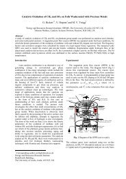
As a first test-case, the bluff-body stabilized flame of
the University of Sydney [17] is considered. The
configuration consists of a burner with a cylindrical
bluff-body with diameter of Db = 50 mm. From the
center of the body, the fuel is ejected into the
surrounding, coflowing air through a nozzle with a
diameter of d = 3.6 mm. The fuel consists of 50% H2
and 50% CH4 by volume.
The geometry is shown in Fig. 1.a, which also indicates
the streamlines of the flow. This configuration has a
complex flow field and strong effects of turbulencechemistry
interaction. In Fig. 1.b a picture of the flame
is shown.
(a) (b)
Fig.1: Geometry of the burner and shape of the bluffbody
stabilized flame
The experiments were carried out for several operating
conditions; in the present paper the HM1E case is
studied, for which the fuel jet has a bulk velocity of 108
m/s and the coflowing air has a velocity of 35 m/s.
The bluff-body stabilized flame was modeled using an
axi-symmetrical, structured grid consisting of 15000
cells. The fuel nozzle was not modeled; the
computational domain starts at the end face of the bluffbody.
The computational has a constant radial width of r
= 1.2 Db and ends downstream at an axial distance of x
= 5 Db from the bluff-body. The defined bulk velocity of
35 m/s is prescribed as an average inlet velocity of the
fuel with a power-law for pipe flow. The inlet
velocities of the coflow were prescribed using the
available measurement data. To account for the round
jet anomaly of the standard k-ε turbulence model, the
Cε1 constant was set to 1.6.

This test case was simulated using non-premixed and
premixed FGM tables as well as using one REDIM
table that was kindly provided to us by Prof. U. Maas.
Since the REDIM table given to us uses 2 2 / CO CO M Y Y =
as a definition of the progress variable, this definition
was for consistency reasons also employed in the nonpremixed
and premixed FGMs used in this study. Using
definitions of the progress variables in the construction
of non-premixed FGMs, which also included the mass
fraction of H2O, CO2, H and/or H2, lead only to minor
improvements in the results. Both FGMs and the
REDIM were tabulated on an equidistant grid with
respectively 201 nodes in the mixture fraction and the
progress variable direction.
In the following a comparison between the simulations
and the experimental data is shown. We are for brevity
omitting the results for the flow field and the results for
the mixture fraction and its variance. It should be noted
that those results are nearly invariant of the chosen
model and are furthermore in a very good agreement
with the measurement data. The interested reader may
however confer the proceedings of the 8 th International
Workshop on Turbulent Nonpremixed Flames [9] for
the computational results of the flow field.
Fig. A1.a-f (on page 6) show the radial profiles of the
simulated and measured temperatures and the mass
fractions CO2 and CO at the axial distances x = 0.26 Db
and x = 1.3 Db. The experimental data are shown in
bullets.
In Fig. A1.a the temperature profiles at the station
closest to the bluff-body are shown. The temperature is
significantly underpredicted on the rich side of the
flame when equilibrium tables are used, as this method
do not account for the diffusion effects, which tend to
raise the temperature on the rich side of non-premixed
flames. All simulations overpredict the temperature and
predict a peak in the temperature in the outer shear layer
at r/Rb≈1. One possible reason for the general
overprediction of the temperature may be due to the
modeling of the end face of the bluff-body as an
adiabatic wall. As can be seen from Fig. A1.b, all
models, except the equilibrium approach, predict the
temperature distributions further downstream
(x/Db=1.3) well.
The Figs. A1.c and A1.d, which show the mass fraction
of CO2, reveal that the use of a premixed FGM leads to
a significant underprediction of the formation of CO2
both close the bluff-body as well as farther downstream,
whereas the flamelet approach only leads to a slight
underprediction. The use of REDIM tables leads to a
slight overprediction of the CO2, whereas the use of
non-premixed FGMs leads to a good agreement
between the computed and measured CO2 mass
fractions at all axial stations. Figs. A1.e and A1.f, in
which the distributions of the mass fraction for the
4
carbon monoxide are displayed, demonstrate that the
simulation using non-premixed FGMs outperform both
the classical flamelet approach as well as the method
using premixed FGMs.
The inferior predictive performance of the premixed
FGM method may be caused by the fact, that the
premixed FGM table is only based on flamelets for
mixture fractions lying between f = 0.02 and f = 0.4.
Outside of this range, the FGM is built by interpolation
between the burning flamelet and the states of the pure
streams. The non-premixed FGMs are on the other hand
based on a library of steady-state flamelets and one
unsteady flamelet that covers all possible values for the
mixture fraction and the progress variable. Thus, for
purely non-premixed combustion, non-premixed FGMs
should preferably be used. It should be noted, that the
limitations of the approach used for the construction of
premixed FGMs will diminish for partially-premixed
configurations and eventually disappear for purely
premixed combustion.
The use of REDIM tables lead only to a fair agreement
between the measurements and our simulations. It
would be worthwhile to investigate if the use of the
REDIM method with another choice for the progress
variable, multiple progress variables and/or the use of
the strain as an additional parameter would yield an
improvement in the predictive performance of the
method.
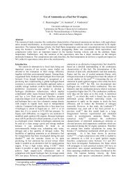
3.2 Generic gas turbine combustor
To assess the models on a test case under partially
premixed conditions, the Generic Gas Turbine (GGT)
combustor of TU Darmstadt was simulated. In this
configuration, preheated, primary air (Tox = 623 K)
enters the combustion chamber through a Turbomeca
swirler nozzle. The combustor is fuelled with pure
methane (Tf = 368 K) and the combustion is operated at
a pressure of 2 bar. After the primary reaction zone,
secondary air is fed into the combustion chamber with a
temperature that equals that of the primary air. Fig. 2
shows a sketch of the test rig.
Fig. 2: Sketch of the GGT combustor testrig [18]
The combustion process in this configuration was
investigated experimentally by Janus [18] and
numerically by Wegner [19]. There are time-resolved

experimental data of the velocity components, the
temperature and the mixture fraction available. By OH
PLIF experiments it has been established, that the flame
in the current test cases exhibits a lifting of
approximately 20 mm.
The combustor including the nozzle was discretized
with a hexahedral mesh consisting of 300.000 cells. To
avoid recirculation at the outlet boundary, the
computational domain was extended by a straight
extrusion of the outlet duct. This case was modeled
using a flamelet library, a non-premixed FGM and a
premixed FGM. For both FGMs the following definition
was used for the progress variable Y:
Y = YCO2
/ M CO2
+ YH
2O
/ M H 2O
In Fig. 3. the predicted temperatures in a cut through the
midplane of the combustor are shown for the flamelet
simulation and for the computation in which a nonpremixed
FGM table was used. The flamelet simulation
predicts that the flame is attached. This result is not
surprising as inherently with the flamelet approach fast
chemistry is assumed. In the simulation in which a nonpremixed
FGM is used, a lifting of the flame is
predicted. The contour plot of the simulation for the
premixed FGM is omitted, as the temperature contours
are very close to that of the flamelet simulations. In Fig.
A2 a comparison between the results of Wegner [19]
using LES and the results obtained in this study with
RANS are shown. The LES results are in good
agreement with the measurements and can thus be used
as a reference. The comparison of computational results
confirms that the use of non-premixed FGMs in the
RANS context lead to a better predictability than when
the flamelet approach is used.
Fig. 3: Simulated temperature distributions in the GGT
combustor using the flamelet and the FGM approach
4. Conclusions
In the present paper the use of various reactednessmixedness
approaches were assessed on a benchmark
flame for purely non-premixed combustion and a
industry-like test case in which partially premixing of
fuel and oxidizer is present. The results show that the
5
non-premixed FGM-approach is more accurate than the
standard flamelet approach. The non-premixed FGMs
account for finite rate effects and are thus able to
accurately resolve the formation of intermediate species
as well as the lifting of partially premixed flames. The
use of REDIM approach and the use of premixed FGM
tables did not prove to have significant advantages over
the use of flamelets. Possible reasons for this have been
explained in the paper. In the on-going work, this will
be investigated further by incorporating test cases for
stratified and premixed flames.
Acknowledgement
The authors would like to thank Prof. U. Maas (ITT,
University of Karlsruhe) for providing us a REDIM
table for the TNF Bluff-body test case. The authors
would also like to thank Mr. Giel Ramaekers, Dr. Jeroen
van Oijen and Prof. de Goey (TU Eindhoven) for
providing us knowledge in the generation of FGM and
training the first author in the use of Chem1D.
Furthermore, the authors are obliged to Dr. Bernhard
Wegner for providing us with results of his LESs.
References
[1] N. Peters, Turbulent Combustion, Cambridge
University Press, 2000
[2] A. Maltsev, PhD Thesis, TU Darmstadt, 2003
[3] J. A. van Oijen, PhD Thesis, TU Eindhoven, 2002
[4] O. Gicquel, N. Darabiha, D. Thevenin, PCI 28
(2000), 1901-1908
[5] B. Fiorina; R. Baron, O. Gicquel, D. Thevenin, S.
Carpentier, N. Darabiha, Combustion Theory and
Modelling 7 (2003), 449 - 470
[6] Z. Ren, S. B. Pope, A. Vladimirsky, J. M.
Guckenheimer, PCI 31 (2007), 473-481
[7] V. Bykov, U. Maas, Combustion Theory and
Modelling 11 (2007), 839-862
[8] A. W. Vreman, B. A. Albrecht, J. A. van Oijen, L.
P. H. de Goey, R. J. M. Baastians, Combust. Flame 153
(2008), 394-416
[9] Proceedings of the TNF workshop, Sandia National
Laboratories, Livermore, CA, www.ca.sandia.gov/TNF.
[10] B. Somers, PhD-thesis, TU Eindhoven, 1994
[11] K. Claramunt, R. Consul, D. Carbonell, C. D.
Perez-Segarra, Combust. Flame 145 (2006), 845-862
[12] H. Pitsch, Combust. Flame 123 (2000), 358-374
[13] U. Maas, S. B. Pope, Combust. Flame 88
(1992), 239-264
[14] A. Jameson, W. Schmidt, E. Turkel, AIAA Paper
81-1259, 1981
[15] C. S. McEnally, L. D. Pfefferle, Combust. Sci.
Technol., 116:183-209, 1996
[16] R. S. Barlow, J. H. Frank, PCI 27 (1998), 1087-
1095
[17] B. Dally, A. Masri, R. S. Barlow, G. Fiechtner,
Combust. Flame 114 (1998), 119-148
[18] B. Janus, PhD Thesis, TU Darmstadt, 2005
[19] B. Wegner, PhD Thesis, TU Darmstadt (2006)

(a) (b)
(c) (d)
(e) (f)
Fig. A1: TNF Bluff-body stabilized flame: Comparison of the computational and the experimental results
Fig. A2: GGT combustor: (Left) mixture fraction, (right) temperature at several axial stations.
Comparison of the RANS results obtained in this study with LES of Wegner [19]
6