Microrheology of Complex Fluid σ = G* ε - OpenWetWare
Microrheology of Complex Fluid σ = G* ε - OpenWetWare
Microrheology of Complex Fluid σ = G* ε - OpenWetWare

Create successful ePaper yourself
Turn your PDF publications into a flip-book with our unique Google optimized e-Paper software.
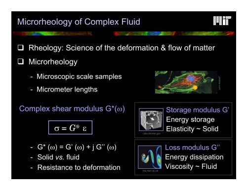
<strong>Microrheology</strong> <strong>of</strong> <strong>Complex</strong> <strong>Fluid</strong><br />
Rheology: Science <strong>of</strong> the deformation & flow <strong>of</strong> matter<br />
<strong>Microrheology</strong><br />
- Microscopic scale samples<br />
- Micrometer lengths<br />
<strong>Complex</strong> shear modulus <strong>G*</strong>(ω)<br />
<strong>σ</strong> = <strong>G*</strong> <strong>ε</strong><br />
- <strong>G*</strong> (ω) = G’ (ω) + j G’’ (ω)<br />
- Solid vs. fluid<br />
- Resistance to deformation<br />
ciks.cbt.nist.gov<br />
ma.man.ac.uk<br />
probes.com<br />
Storage modulus G’<br />
Energy storage<br />
Elasticity ~ Solid<br />
Loss modulus G’’<br />
Energy dissipation<br />
Viscosity ~ <strong>Fluid</strong>
High Frequency <strong>Microrheology</strong> Measurement<br />
Active Method:<br />
Magnetic microrheometer – Baush, BJ 1998<br />
Huang, BJ 2002<br />
Passive Method:<br />
Single particle tracking – Mason, PRL 1995<br />
Yamada, BJ 2000<br />
Multiple particle tracking – Crocker, PRL 2000
Magnetic <strong>Microrheology</strong><br />
Magnetic <strong>Microrheology</strong> 5 sec Step Response
Basic Physics <strong>of</strong> Magnetic Microrheometer<br />
Ferromagnetic particle<br />
1<br />
F = µ ∇( m⋅H) 2 0<br />
Paramagnetic particle – no permanent magnetic moment<br />
F = µ χV<br />
∇( H⋅H) 0<br />
Note: (1) force depends on volume <strong>of</strong> particle<br />
(5 micron bead provide 125x more force)<br />
(2) force depends on magnetic field GRADIENT<br />
Particles cluster together!<br />
Doesn’t work!<br />
χ is suceptibility<br />
V is volume
Magnetic manipulation in 3D<br />
*Lower Force<br />
nN level<br />
*3D<br />
*Uniform gradien<br />
Amblad, RSI 1996<br />
Huang, BJ 2002
Magnetic manipulation in 1D<br />
Baush, BJ 1998<br />
*High force<br />
>10 nN<br />
*Field non-uniform<br />
Needs careful<br />
alignment <strong>of</strong> tip<br />
to within microns<br />
The bandwidth <strong>of</strong> ALL magnetic microrheometer is limited by the inductance<br />
<strong>of</strong> the eletromagnet to about kiloHertz<br />
*1D
Magnetic Rheometer Requires Calibration<br />
Baush, BJ 1998
Mag Rheometer Experimental Results<br />
Baush, BJ<br />
1998<br />
Transient responses allow fitting<br />
to micro-mechanical model<br />
Problem – Magnetic bead rolling<br />
Solution – Injection, Endocytosis<br />
Modeling (Karcher BJ 2003)
Model Strain Field Distribution<br />
Baush, BJ 1998
Single Particle Tracking<br />
Consider the thermal driven motion <strong>of</strong> a sphere in a complex fluid<br />
Langevin Equation<br />
Inertial<br />
force<br />
t<br />
mv&<br />
( t)<br />
= f ( t)<br />
+ ∫ξ ( t − t')<br />
v(<br />
t')<br />
dt'<br />
Random<br />
thermal<br />
force<br />
0<br />
Memory function—<br />
Material viscosity<br />
Particle shape
Langevin Equation in Frequency Domain<br />
v~<br />
( s)<br />
=<br />
Laplace transform <strong>of</strong> Langevin Equation<br />
~<br />
f ( s)<br />
+ mv(<br />
0)<br />
~<br />
ξ ( s)<br />
+ ms<br />
Multiple by v(0),<br />
taking a time average,<br />
Ignoring inertial term<br />
~<br />
G(<br />
s)<br />
=<br />
kT<br />
< ∆~<br />
2<br />
πas<br />
r ( s)<br />
><br />
Random force<br />
<<br />
~<br />
f ( s)<br />
v(<br />
0)<br />
>=<br />
0<br />
Equipartition <strong>of</strong> energy<br />
m < v(<br />
0)<br />
v(<br />
0)<br />
>= kT<br />
Generalized Stokes Einstein<br />
ξ ( s)<br />
= 6πa<br />
~ η ( s)<br />
< v(<br />
0)<br />
v~<br />
( s)<br />
>= s<br />
2<br />
~<br />
G(<br />
s)<br />
= s<br />
~ η ( s)<br />
Definition and Laplace transform<br />
<strong>of</strong> mean square displacement<br />
< ∆~<br />
r<br />
2<br />
( s)<br />
> / 6
(2) Fluorescence Laser Tracking<br />
Microrheometer<br />
• Approach: Monitoring the Brownian dynamics <strong>of</strong> particles<br />
embedded in a viscoelastic material to probe its frequencydependent<br />
rheology<br />
Yamada, Wirtz, Kuo, Biophys. J. 2000<br />
Ch0<br />
Ch2<br />
Ch1<br />
Ch3<br />
trajectory<br />
mean squared displacement<br />
shear modulus
(2) Nanometer Resolution for the Bead’s<br />
Trajectory<br />
• Collecting enough light from a fluorescent bead is critical<br />
Photons detected<br />
per measurement<br />
A B<br />
xc <strong>σ</strong> = 0.5 µm<br />
x<br />
10 3 10 4 10 5 10 6<br />
Uncertainty on 0.033 0.010 0.003 0.001<br />
Uncertainty on x c (nm) 12 4 1.2 0.4<br />
Nanometer resolution ↔ 10 4 photons per measurement
(2) Calibrating the FLTM<br />
y<br />
x<br />
Ch3<br />
Ch1<br />
Ch2<br />
Ch0<br />
• 5-nm stepping at 5 or 50 kHz • Curve fitting matches theory
Characterizing the FLTM<br />
• Using polyacrylamide gels (w/v 2% to 5%) <strong>of</strong> known properties<br />
Good agreement with previously published data<br />
Schnurr B., Gittes F., MacKintosh F.C. & Schmidt C.F<br />
Macromolecules (1997), 30, p.7781-7792
Single Particle Tracking Data<br />
Yamada BJ 2000
Two- and Multiple Particle Tracking<br />
SPT responses can be influence by local processes (adhesion, active, etc)<br />
and not represents global cytoskeleton behavior<br />
Solution: Look at the correlated motion <strong>of</strong> two particles under thermal force<br />
D<br />
D<br />
rr<br />
rr<br />
i<br />
r<br />
( r,<br />
τ ) =< ∆r<br />
( t,<br />
τ ) ∆r<br />
( t,<br />
τ ) δ ( r − R ( t))<br />
> ≠ ,<br />
( r,<br />
s)<br />
=<br />
kT<br />
~<br />
2πrsG(<br />
s)<br />
j<br />
r<br />
Instead <strong>of</strong> using fast quadrant detectors, multiple particle<br />
tracking uses a wide field camera which is slower<br />
ij<br />
i<br />
j<br />
t<br />
The major difference<br />
is that the correlation<br />
signal is a function<br />
<strong>of</strong> “r” the separation<br />
<strong>of</strong> the particles but<br />
not their size
SPT vs MPT<br />
Crocker, PRL 2000<br />
Triangle: SPT<br />
Circle: MPT<br />
SPT and MPT results<br />
can be quite different<br />
specially in cells
A Comparison <strong>of</strong> Microrheometry Methods<br />
Bandwidth<br />
Signal<br />
Amplitude<br />
Local Effects<br />
Nonlinear<br />
regime<br />
Instrument<br />
Magnetic<br />
kHz<br />
µm<br />
Yes<br />
Yes<br />
Intermediate<br />
SPT<br />
MHz<br />
nm<br />
Yes<br />
No<br />
Intermediate<br />
MPT<br />
kHz<br />
nm<br />
No<br />
No<br />
Simple