Random Recurrent Neural Networks Dynamics - BSTU Laboratory ...

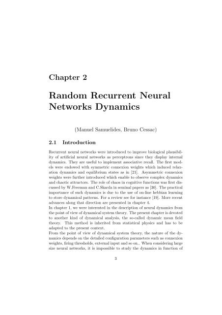
Chapter 2 

Random Recurrent Neural 

Networks Dynamics 

2.1 Introduction 

(Manuel Samuelides, Bruno Cessac) 

Recurrent neural networks were introduced to improve biological plausibility 

of artificial neural networks as perceptrons since they display internal 

dynamics. They are useful to implement associative recall. The first models 

were endowed with symmetric connexion weights which induced relaxation 

dynamics and equilibrium states as in [21]. Asymmetric connexion 

weights were further introduced which enable to observe complex dynamics 

and chaotic attractors. The role of chaos in cognitive functions was first discussed 

by W.Freeman and C.Skarda in seminal papers as [30]. The practical 

importance of such dynamics is due to the use of on-line hebbian learning 

to store dynamical patterns. For a review see for instance [19]. More recent 

advances along that direction are presented in chapter 4. 

In chapter 1, we were interested in the description of neural dynamics from 

the point of view of dynamical system theory. The present chapter is devoted 

to another kind of dynamical analysis, the so-called dynamic mean field 

theory. This method is inherited from statistical physics and has to be 

adapted to the present context. 

From the point of view of dynamical system theory, the nature of the dynamics 

depends on the detailed configuration parameters such as connexion 

weights, firing thresholds, external input and so on.. When considering large 

size neural networks, it is impossible to study the dynamics in function of 

3

4CHAPTER 2. RANDOM RECURRENT NEURAL NETWORKS DYNAMICS 

the whole set of detailed configuration parameters because its dimensionality 

is too large. One may consider that the detailed parameters share few 

generic values but it does not allow to study the effect of their variability. We 

consider here random models where the detailed configuration parameters 

as connexion weights form a random sample of a probability distribution. 

These models are called ”Random Recurrent Neural Networks”(RRNN). In 

that case, the parameters of interest define the probability distribution of 

the detailed configuration parameters. They are statistical parameters and 

have been introduced as ”macroscopic parameters” in Chapter 1. Then the 

dynamics is amenable because one can approach it by ”Mean-Field Equations” 

(MFE) as in Statistical Physics. So, study of the dynamics in terms of 

relevant dynamical quantities, called ”order parameters” can be performed. 

Mean-Field Equations were introduced for neural networks by Amari [2] and 

Crisanti and Sompolinsky [31]. We extended their results [10] and used a 

new approach to prove it in a rigorous way [27]. This approach is the ”Large 

deviation Principle” (LDP) and comes from the rigorous statistical mechanics 

[5]. Simultaneously, mean-field equations were successfully used to 

predic the dynamics of spiking recurrent neural networks. Though there is 

no rigorous background to support these new developments, the success of 

this approach deserves new investigations. This chapter intends to provide a 

bridge between the detailed computation of the asymptotic regime and the 

rigorous theory which is shown to support in at least in some models MFE 

theory. 

In section 2, the various models are stated from the points of view of the 

single neuron dynamics and of the global network dynamics. A summary 

of notations is presented, which is quite helpful for the sequel. In section 3 

mean-field dynamics is developped and it is shown to be a fixed point of the 

mean-field propagation operator. The global dynamics probability distribution 

is computed and the associate empirical measure is proven to converge 

with exponential rate towards mean-field dynamics. The mathematical tools 

which are used there are detailed (without any proof) in appendix, section 

6. In section 4, some applications of mean-field theory to the prediction of 

chaotic regime for analog formal random recurrent neural networks (AFR- 

RNN) are displayed. The dynamical equation of homogeneous AFRRNN 

which is studied in chapter 1 is derived from the random network model 

in section 4.1. Moreover a two-population model is studied in section 4.2 

and the occurence of a cyclo-stationary chaos is displayed using the results 

of [11]. In section 5, an insight of the application of mean-field theory to

2.2. DYNAMICS OF RRNNN 5 

IF networks is given using the results of [7]. The model of this section is a 

continuous-time model following the authors of the original paper. Hence 

the theoretical framework of the beginning of the chapter has to be enlarged 

to support this extension of mean-field theory and this work has to be done. 

However, we sketch a parallel between the two models to induce further 

research. 

2.2 Dynamics of RRNNN 

2.2.1 Defining dynamic state variables 

We first reconsider in a stochastic context some notions that have been 

acquired in Chapter 1. In a stochastic model, all state variables may be 

considered as random variables. 

We study here discrete time dynamics and restrain ourselves to finite timehorizon. 

In that section, we shall study the case of homogeneous neural networks. 

More realistic cases such as several population networks will be considered 

further on. Though we are really interested in long-time behaviour 

and stationary regime if any, rigorous proofs of convergence of large-size 

networks only exist for finite time. Thus we consider time t as an integer 

belonging to time interval {0, 1, ..., T } where the integer T stands for the 

horizon. 

Since the model is stochastic, all state variables may be considered as random 

variables. The change of probability distributions are common in that 

chapter whether it occurs from conditioning or from changing basic assumption 

over dynamics. Anyhow, we won’t change notation for the random 

variables. Moreover following the standard physicist’s habit, the random 

variables won’t be noted by capital letters. 

The state of an individual neuron i at time t is described by an instantaneous 

individual variable, the membrane potential ui(t). Here, ui(t) is a real 

random variable which takes its value in R. So an individual state trajectory 

ui =(ui(t)) t∈{0,1,...,T } takes its value in F = R {0,1,...,T } . We shall generally 

prefer to study the distribution of a trajectory than the instantaneous state 

distribution. The second order moments of an individual trajectory ui are 

its expectation E(ui) ∈F and its covariance matrix Cov(ui) ∈F⊗F. 

Our aim is to study the coupled dynamics of N interacting neurons that 

constitue a neural network. N is the size of the neural network. The global 

state trajectory of u =(ui) i∈{1...,N} is a random vector in F N . The prob-


ability law 1 QN of the random vector u depends on N. We shall compute 

this law for various neuron models in this section. 

As it was detailed in the previous chapter, the dynamics of the neuron 

models we study here depends on three basic assumptions 

• about how the neuron activation depends on the membrane potential, 

• about how the other neurons contribute to the synaptic potential 

which summarizes completely the influence of the network onto the 

target neuron, 

• about how the synaptic potential is used to update the membrane 

potential. 

We shall now detail these points in the models that are considered further 

on. 

2.2.2 Spike emission modeling 

It is considered that the neuron is active and emits a spike when its membrane 

potential exceeds the activation threshold. So the neuron i is active 

at time t when ui(t) ≥ θ where θ is the neuron activation threshold. We 

consider here that θ is a constant of the model which is the same for all 

neurons. Actually this hypothesis may be relaxed and random thresholds 

may be considered but the notation and the framework of dynamical study 

would be more complicate (see [27]). 

For spiking neuron models we define an activation variable xi(t) which is 

equal to 1 if neuron i emits a spike at time t and to 0 otherwise. Hense we 

have 

xi(t) =f[ui(t) − θ] (2.1) 

where f is the Heaviside function which is called the transfer function of 

the neuron. Actually, to alleviate notations, we shift ui of θ and that allows 

to replace equation (transfer0.eq) by equation 

xi(t) =f[ui(t)] (2.2) 

The threshold will be further taken into account in the updating equation. 

Two spiking neuron models are considered here, the Binary Formal neuron 

(BF) which is the original model of Mac Culloch aand Pitts [25] and 

1 This term is defined in Appendix, definition 2.7


the Integrate and Fire neuron (IF) which is generally used nowadays 

to model dynamics of large spiking neural networks [17]. 

In these models, the neuron activation takes generally two values: 0 and 1. 

This is true for most models of neurons. However, it was preferred in a lot 

of research works to take into account the average firing rate of the model 

instead of the detailed instant of firing. This point of view simplifies the 

model and deals with smooth functions which is easier from a mathematical 

point of view. According this point of view equation (2.2) is still valid but 

xi(t) takes its values in the interval [0, 1] and the transfer function f is a 

smooth sigmoid function for instance f(x) = ex 

. Since the activation of 

1+ex then euron is represented by a real vaue that varies continuously, the model 

is called Analog Formal neuron (AF) 

AF model is still widely dominant when Artificial Neural Networks are considered 

for applications since gradient are easy to compute. For biological 

purpose, it was widely believed that the relevant information was stored in 

the firing rate; in that case more precise modeling would not be so useful, 

at least from a functional point of view. The three models are studied in 

that chapter and we attempt to give a unified presentation of mean-field 

equation for these three models. 

Notice that the state of the neuron is the membrane potential ui(t) and 

not the activation xi(t). This is due to the update law of the IF model. We 

shall retun to that point further. 

2.2.3 The synaptic potential of RRNN 

The spikes are used to transmit information to other neurons through the 

synapses. Let us note J =(Jij) the system of synaptic weights. At time 

0, the dynamic system is initialized and the synaptic potentials are null. 

The synaptic potential of neuron i of a network of N neurons at time 

t + 1 is expressed in function of J and u(t) ∈ R N by 

vi(J ,u)(t +1)= 

N 

Jijxj(t) = 

j=1 

N 

Jijf[uj(t)] (2.3) 

When considering large size neural networks, it is impossible to study the 

dynamics in function of the detailed parameters. One may consider that 

the connexion weights share few values but it does not allow to study the 

effect of the variability. We consider here random models where the connexion 

weights form a random sample of a probability law. These models are 

called ”Random Recurrent Neural Networks”(RRNN). In that case, 

j=1


the parameters of interest are the order parameters i.e. the statistical parameters. 

For size N homogeneous RRNN model with gaussian connexion 

weights, J is a normal random vector with identically distributed independent 

components. The common law of the components is a normal law 

N ( υ υ2 

N , N ). The order parameters of the model are υ and υ. 

Note that the assumption of independence is crucial in the approach described 

below. Unfortunately, the more realistic case where correlations 

between the Jijs exist (e.g. after Hebbian learning) is not currently covered 

by the mean-field methods. The description of the hebbian learning process 

in the stochastic RRNN framework has to be discovered in the future 

research. 

In the sequel, we shall extend the RRNN model properties to a more general 

setting where the weights are non gaussian and depend on the neuron class 

in a several population model like in [11]. 

We have already dealt with the dynamical properties of RRRN such as (1.3). 

In Chapter 1, we fixed a realization of J and considered the evolution of 

trajectories of this dynamical system. Then, we averaged over J distribution 

in order to get informations about the evolution of averaged quantities. 

In the present chapter we shall start with a complementary point of view. 

Namely, assume that we fix a network state trajectory u. Let us consider 

the vector vi(J ,u)=(vi(J ,u)(t)) ∈Fwhich is the trajectory of the synaptic 

potential. When u is given, since the synaptic weights Jij are gaussian, 

identically distributed and independant we infer that the vi(., u) are identically 

distributed normal independent random vectors in F (see in appendix 

proposition (2.17). The distribution of the vi is defined by its mean mu and 

its covariance matrix cu. 

We have 

mu(t +1)= υ 

N 

f[(uj(t)] (2.4) 

N 

and 

cu(s +1,t+1)= υ 

N 

j=1 

N 

f[(uj(s)]f[(uj(t)] (2.5) 

Notice that these parameters are invariant by any permutation of the neuron 

membrane potentials. Actually, they depend only on the empirical 

distribution 2 µu, which is associated to u. µ is a probability law on F. It 

just weights equally each individual neuron state trajectory. 

j=1 

2 This concept is introduced in the appendix in definition (2.18)


Definition 2.1 The empirical measure µu is an application from F N on 

P(F ), the set of probability measures on F which is defined by 

µu(A) = 

N 

i=1 

δui (A) (2.6) 

where δui (A) is the Dirac mass on individual trajectory ui such that δui (A) = 

1ifui belongs to A and 0 otherwise. Using this formalism provides an 

useful way to perform an average over the empirical distribution of the 

whole network. More generally, assume that we are given a probability law 

µ on the indivudual trajectory space F. Then, one can perform a generic 

construction of a gaussian distribution on RT by 

Definition 2.2 For any µ ∈P(F) the gaussian probability law gµ on RT with moments mµ and cµ that are defined by : 

 

mµ(t +1)=υ f[η(t)]dµu(η) 

cµ(s +1,t+1)=υ2 (2.7) 

f[η(s)]f[η(t)]dµu(η) 

Then, it is easy to reformulate the previous computation as: 

Proposition 2.1 The common probability law of the individual synaptic 

potential trajectories vi(., u) is the normal law gµu where µu is the empirical 

distribution of the network potential trajectory u. 

Proposition 2.2 The common probability distribution of the individual synaptic 

potential trajectories vi(., u) is the normal law gµu where µu is the empirical 

distribution of the network potential trajectory u. 

This framework is useful to compute the large-size limit of the common 

probability law of the potential trajectories. 

2.2.4 Dynamical models of the membrane potential 

We shall now detail the updating rule of the membrane potential. Various 

neural dynamics have been detailed in thep revious chapter. We focus here 

on two dynamics formal neuron (AF and BF) and Integrate and Fire neuron 

(IF). 

For the two models, the network is initialized with indepedent identically 

distributed membrane potential according to a probability law µinit ∈P(R). 

We introduce for each neuron i, a sequence (wi)(t)) t∈{1,...,T } of i.i.d. centered 

Gaussian variables of variance σ 2 . This sequence is called the synaptic


noise of neuron i and stands for all the defects of the model. The synaptic 

noise plays an important part in the mathematical proof but the order parameter 

σ is as small as necessary. So this model is not very restrictive. The 

synaptic noise is added to the synaptic potential. Of course the synaptic 

noises of the neurons are independent altogether. In some papers, the synaptic 

noise is called thermal noise by comparison with the random variables 

J =(Jij), which are called quenched variables as they are fixed, once for 

all and do not change with time. 

Recall that formal neuron updates its membrane potential according to 

ui(t +1)=vi(t +1)+wi(t +1)− θ (2.8) 

IF neuron takes into acccount its present membrane potential while updating. 

Its evolution equation is 

where 

ui(t +1)=ϕ[ui(t)+θ)] + vi(t +1)+wi(t +1)− θ (2.9) 

• γ ∈]0, 1[ is the leak 

• ϕ is defined by 

ϕ(u) = 

• ϑ is the reset potential and ϑ


and so P = µinit ⊗N(−θ, σ 2 ) ⊗T . In the case of IF neurons P is not explicit. 

It is the image of µinit ⊗N(−θ, σ 2 ) ⊗T by the diffusive dynamics 

ui(0) ∼ µinit, ui(t +1)=ϕ[ui(t)+θ)] + wi(t +1)− θ (2.12) 

When coupling the neurons, the network trajectory is still a random vector. 

Its probability distribution, which is denoted by QN, has a density with 

respect to P ⊗N that can be explicitely computed. This is the main topic of 

the next subsection. 

2.2.5 Computation of the network dynamics law 

This section is dedicated to the computation of the probability distribution 

QN. The result shows that the density of QN with respect to free dynamics 

probability P ⊗N depends on the trajectory variable u only through the 

empirical measure µu. To achieve this computation we shall use a key result 

of stochastic process theory, the Girsanov theorem which gives the density 

of the new law of a diffusion when the trend is changed. Actually, since 

the time set is finite, the version of Girsanov theorem we use is different 

and may be recovered by elementary gaussian computation. Its derivation 

is detailed in the appendix in theorem 2.20. A similar esult may be obtained 

for continuous time dynamics using the classical Girsanov theorem (see [5]). 

Let us state the finite-time Girsanov theorem 

Theorem 2.3 Let µinit a probability measure on Rd and let N (α, K) be 

a gaussian regular probability on Rd . Let T a postive integer and ET = 

(Rd ) {0,...,T } the space of finite time traajectories in Rd . Let w a gaussian 

random vector in ET with law µinit ⊗N(α, K) T .Letφand ψ two measurable 

applications of Rd into Rd . Then we define the random vectors x and y in 

E by 

 

x0 = w0 

x(t +1)=φ[x(t)] + w(t +1) 

 

y0 = w0 

y(t +1)=ψ[y(t)] + w(t +1) 

Let P and Q be the respective probability laws on E of x and y, then Q is 

absolutely continuous with respect to P and we have 

T 

dQ −1 

1 − 

(η) = exp 

2 

dP 

t=0 

{ψ[(η(t)] − φ[(η(t)]}tK −1 {ψ[(η(t)] − φ[(η(t)]} 

+{ψ[(η(t)] − φ[(η(t)]} tK −1 

{η(t +1)−α − φ[η(t)]} 

(2.13)


We shall use this theorem to prove the following: 

Theorem 2.4 The density of the law of the network membrane potential 

QN with respect to P ⊗N is given by 

Γ(µ) = log 

with 

dQN 

dP ⊗N (u) = exp NΓ(µu) 

where the functionnal Γ is defined on P(F) by 

exp 1 

σ 2 

T −1 

t=0 

− 1 

2 ξ(t +1)2 +Φt+1(η)ξ(t +1) dgµ(ξ) 

• for AF and BF models: Φt+1(η) =η(t +1)+θ 

• IF model: Φt+1(η) =η(t +1)+θ − ϕ[η(t)+θ] 

 

dµ(η) 

(2.14) 

Remark 2.1 Let us recall that the gaussian measure gµ has been defined 

previously (Definition 2.2) 

PROOF OF THEOREM: We note QN(J ) the conditional law of the network 

state trajectory given J the system of synaptic weights. We shall apply the 

finite-time Girsanov theorem 2.3 to express dQN (J ) 

dP ⊗N . To apply the theorem 

we notice that 

• The difference of the two trend terms ψ[η(t) − φ[η(t)] of the theorem 

is here the synaptic potentials (vi(t)). The synaptic potentials vi are 

functions of the ui according to (2.3) 

vi(J ,u)(t +1)= 

N 

Jijf[uj(t)] 

• The expression of the synaptic noise (wi(t + 1) in function of the state 

trajectory uiin the free dyamics is Φt+1(ui) which expression depends 

on the neuron model (formal or IF). 

We have so 

dQN(J ) 1 

(u) = exp 

dP ⊗N σ2 T −1 

t=0 

N 

i=1 

j=1 

 

− 1 

2 vi(J ,u)(t +1) 2 

+ vi(J ,u)(t + 1)Φt+1(ui) 

(2.15)


dQN(J ) 

(u) = 

dP ⊗N 

N 

i=1 

exp 1 

σ 2 

T −1 

t=0 

 

− 1 

2 vi(J ,u)(t +1) 2 

+ vi(J ,u)(t + 1)Φt+1(ui) 

(2.16) 

Now let us consider the probability of the quenched variables J =(Jij). 

We observed previously when we introduced the synaptic potential model 

that under the configuration distribution of J , the random vectors vi(J ,u) 

are independent identically distributed according to the normal law gµu 

To compute the density of QN with respect to P ⊗N one has to average the 

conditional density dQN (J ) 

dP ⊗N over the configuration distribution of J . the 

integration separates into products and one gets from (2.16) the following 

dQN 

(u) = 

dP ⊗N 

dQN 

(u) = exp 

dP ⊗N 

N 

i=1 

N 

 

i=1 

 

log 

exp 1 

σ 2 

exp 1 

σ 2 

T −1 

t=0 

T −1 

t=0 

 

− 1 

2 ξ(t)2 

+Φt+1(ui)ξ(t) dgµu(ξ) 

 

− 1 

2 ξ(t +1)2 

+Φt+1(ui)ξ(t +1) dgµu(ξ) 

The sum over i is equivalent to an inegration over the empirical measure µu, 

so we have 

dQN 

(u) = exp N log exp 

dP ⊗N 1 

σ2 T −1 

− 1 

2 ξ(t +1)2 

+Φt+1(η)ξ(t +1) dgµu(ξ) dµu(η) 

Remark 2.2 

t=0 

Equation 2.14 reminds the generating functional approach derived e.g. by 

Sompolinsky al. [31] or Molgedey al [24] which allows to compute the 

moments of ui(t). However, the present approach provides a stronger result. 

While the generating functional method deals with weak convergence 

(convergence of generating function) the method that is developped here 

allows direct access to ui(t)s probability distribution. Moreover, using large 

deviation techniques provides almost sure convergence results. This convergence 

is valid for only one typical sample. This property is also called 

self-averaging in the statistical physics community. Let us now state an important 

corollary of this theorem which will be the basic statement for the 

convergence theorem of next section.


Corollary 2.5 The density of the law of the empirical measure µu as a 

random measure in the RRNN model that is governed by QN with respect to 

the law of the empirical measure in the free model that is governed by P ⊗N 

is 

2.2.6 Summary of notations 

µ ∈P(F) → exp NΓ(µ) 

Let us recall the notations of this section. They will be extensively used in 

the following sections: 

Notation Interpretation 

i ∈{1, ..., N} individual neuron of a N neuron population 

t ∈{0, ..., T } time course of the discrete time dynamics at horizon T 

ui(t) membrane potential of neuron i at time t 

xi(t) activation state of neuron i at time t 

vi(t) synaptic potential of neuron i at time t 

wi(t) synaptic summation noise of neuron i at time t 

ui ∈F membrane potential trajectory of neuron i from time 0 to time T 

u ∈F N network membrane potential trajectory i from time 0 to time T 

xi ∈E activation state trajectory of neuron i from time 0 to time T 

x ∈F N network activation state trajectory from time 0 to time T 

θ common firing threshold of individual neurons 

σ common standard deviation of the synaptic noise 

λ leak current factor for Integrate and fire (IF) neuron model 

f neuron transfer function converts membrane potential into activation state 

Jij synaptic weight from neuron j to neuron i (real random variable) 

J =(Jij) synaptic weight matrix (random N × N matrix) 

υ 

N 

υ 

expectation of synaptic weights Jij 

2 

N 

µ ∈P(F) 

variance of synaptic weights Jij 

generic probability law of individual membrane potential trajectory 

η ∈F random vector which takes its values in F under probability law µ 

P ∈P(F) probability law of individual membrane potential trajectory for free dynamics 

gµ ∈P(F) synaptic potential law obtained from µ ∈P(F ) through central limit approximation 

QN ∈P(FN ) probability law of network membrane potential trajectory u

2.3. THE MEAN-FIELD DYNAMICS 15 

2.3 The mean-field dynamics 

2.3.1 Introduction to mean-field theory 

The aim of this section is to describe in the limit of large size networks the 

evolution of a typical neuron by summarizing in a single term the effect of 

the interactions of this neuron with the other neurons of the network. Such 

an approximation will be valid through an averaging procedure which will 

take advantage of the large number of coupling to postone the vanishing 

of individual correlations between neurons or between neurons and configuration 

variables. This is the hypothesis of ”local chaos” of Amari ([1],[2]), 

or of ”vanishing correlations” which is usually invoked to support meanfield 

equations. The ”mean-field” is properly the average effet of all the 

interaction of other neurons with the neuron of interest. This approach is 

currently used in statistical mechanics since Boltzmann and the assumption 

is also kown under ”molecular chaos”. 3 

So the mean field dynamics is intermediate between the detailed dynamics 

which takes into account all the detailed interactions between neurons and 

the free dynamics which neglects all the interaction. In mean-field theory, we 

are looking for an evolution equation of the type of free dynamics equation 

that are involving single neuron dynamics but were the interaction term is 

not cancelled. To do that we shall replace vi(t) by an approximation which 

depends only on the statistical distribution of the uj(t). The approximation 

of vi =(vi(t)) ∈Fwill be called the mean-field and will be noted ζ = 

(ζ(t)) ∈F. The important assumption to derive the anzats is: 

In the large size limit, uj are asymptotically independent, they 

are also independent from the configuration parameters 

From the central limit theorem we are then allowed to postpone that ζ is 

approximatively a large sum of independent identically distributed variable, 

and thus that it follows approximatively a Gaussian law. We have just to 

derive its first and second order moment from the common probability law 

of ui =(ui(t)) to know completely the distribution of ζ. 

Thus from a probability law on F which is supposed to be the common 

3 The word ”chaos” is somehow confusing here, especially because we also dealt with 

deterministic chaos in the first chapter. Actually, ”deterministic chaos” and the related 

exponential correlation decay is connected to the mean-field approaches which allows to 

compute deterministic evolution equation for the mean value and Gaussian fluctuations. 

However, here the mean-field approach works basically because the model is fully connected 

and the Jij are vanishing in the large-size limit. This is standard result in statistical 

physics models such as the Curie-Weiss model but obtaining this for the trajectories 

of a dynamical model with quenched disorder requires more elaborated technics.


probability law of the ui, we are able to derive the law of ζ and then the law 

of the resulting potential trajectory and of the state trajectory of a generic 

vector of the network. In that way, we are able to define an evolution 

operator L on the set P(F ) of the probability laws on F which we call the 

mean-field propagation operator. 

2.3.2 Mean-field propagation and mean-field equation 

Let µ ∈P(F) be a probability measure on F and let us compute the moments 

of 

N 

∀t ∈{0, 1, ..., T − 1},ζ(t +1)= Jijf[uj(t)] 

where the uj are independent identically distributed random vectors with 

probability law µ and independent from the configuration parameters Jij. 

Since E[Jij] = υ 

N and Var[Jij] = υ2 

N ,wehave 

 

E[ζ(t + 1)] = υ F f[η(t)]dµ(η) 

 

Cov[ζ(s +1),ζ(t + 1)] = υ2 E f[η(s)]f[η(t)]dµ(η) 

(2.17) 

Notice that the expression of the covariance is asymptotic since the sum of 

squares of expectation of the synaptics weights may be neglected. So ζ is a 

Gaussian random vector in F with probability law gµ (see definition 2.2). 

Definition 2.3 Let µ a probability law on F such that the law of the first 

component is µinit. Letu, w, v be three independent random vectors with the 

following laws 

• the law of u is µ, 

• the law of w is N (0,σ 2 IT ), 

• the law of v is gµ 

Then L(µ) is the probability law on F of the random vector ϑ which is defined 

by 

ϑ(0) = u(0) 

ϑ(t +1)=v(t +1)+w(t +1)−θ (2.18) 

for the formal neuron models (BF and AF), and by 

 

ϑ(0) = u(0) 

ϑ(t +1)=ϕ[u(t)+θ)] + v(t +1)+w(t +1)−θ (2.19) 

for the IF neuron model. The operator L which is defined on P(F) is called 

the mean-field propagation operator. 

j=1


Definition 2.4 The following equation on µ ∈P(F) 

is called the mean-field equation (MFE) 

L(µ) =µ (2.20) 

Remark 2.3 The mean-field equation is the achievement of mean-field approach. 

To determine the law of an individual trajectory, we suppose that 

this law governs the interaction of all the units onto the selected one, the 

resulting law of the selected unit has to be the same law than the generic 

law. This is summarized in the mean field equation 

L(µ) =µ 

Equations 2.18 (resp. (2.19) for the IF model) with the specification of the 

probability laws define the mean-field dynamics. Actually, the law L(µ) 

is just the convolution of the probability laws P and the gaussian law gµ. 

More precisely, if we apply the discrete time Girsanov theorem 2.20 of the 

appendix, we have: 

Theorem 2.6 L(µ) is absolutely continuous with respect to P and it density 

is given by 

 

dL(µ) 

(η) = 

dP 

exp 1 

σ 2 

T −1 

t=0 

 

− 1 

2 ξ(t +1)2 

+Φt+1(η)ξ(t +1) dgµ(ξ) (2.21) 

PROOF : The proof is essentially a simplified version of the application of the 

finite-time Girsanov theorem which was used to prove theorem (2.4). The 

conditioning is done here with respect to v which is the difference between 

the trend terms of the free dynamics and of the mean-field dynamics. 

Remark 2.4 We have to notice for further use that 

 

Γ(µ) = log dL(µ) 

(η)dµ(η) 

dP 

(2.22) 

In all the cases, for 0


Theorem 2.7 The probability measure µT =L T (P ) is the only solution of 

the mean-field equation with initial condition µinit. 

2.3.3 LDP for RRNN mean-field theory 

In this section, we fully use the computation results of the previous section to 

show the rigorous foundations of mean-field theory for RRNN. The approach 

is the following: 

(a) The empirical measure µu of the network dynamics satisfies a large 

deviation principle (LDP) under P ⊗N with the good rate function 

µ ∈P(F) → I(µ, P ) ∈ R + . Actually, when the size of the network 

goes to infinity, the empirical measure converges in law exponentially 

fast towards P . The definition of LDP and its consequences are outlined 

in the appendix in definition 2.16. Sanov theorem is stated in 

appendix, theorem 2.25. 

(b) According to corollary 2.5, the density of the new law of µu with 

respect to the original law when we switch from P ⊗N that governs the 

free dynamics to QN that governs the RRNN dynamics is exp NΓ(µ). 

(c) Combining (a) and (b), one obtains that under QN, the sequence µu 

satisfies a LDP with the good rate function 

H(µ) =I(µ, P ) − Γ(µ) (2.23) 

This kind of result is used in statistical physics under the name of 

Gibbs variational principle [16]. The functional H is called the 

free energy. Notice, that the classical statistical mechanics framework 

is relative to equilibrium state. It is applied here for state trajectory. 

For that reason, this approach is called the dynamic meanfield 

theory [31]. Here, it is be quite technical to support it rigorously. 

One has to show that H is is lower semi-continuous and is a good rate 

function (see Varadhan’s theorem 2.24 of the appendix). This kind of 

proof is rather technical (see [5] for a general approach and [27] for the 

proof for AFRRNN model). So we admit the following result 

Theorem 2.8 Under the respective laws QN the family of empirical 

measures (µN) of P(F) satisfies a full large deviation principle with 

the good rate function H


(d) It is clear from remark 2.4 that H(µT ) = 0 where µT is is the unique 

solution of MFE with initial condition µinit, so it is the fixed point of 

L. Thus µT is a minimum of H. 

The basic computation is the following: first we apply the definition 

2.19 of the relative entropy that is given in in the appendix 

 

I(µT ,P)= 

Since µT is the solution of MFE, we have 

log dµT 

dP (η)dµT (η) 

dµT 

dP (η) =dL(µT ) 

dP (η) 

then we apply the previous remark 2.4 which states 

to check 

 

Γ(µT )= 

log dL(µT ) 

dP (η)dµT (η) 

I(µT ,P)=Γ(µT ) ⇒ H(µT )=0 

(e) To obtain the exponential convergence of the sequence of empirical 

measures µu under QN when N →∞, one has eventually to show 

that H(µ) =0⇒ µ = µT . This point is technical too. It is proved in 

a similar still more general framework (continuous time) in [5] using 

a Taylor expansion. The same method is and applied to show the 

unicity for AFRRNN model in [27]. 

Thus, we have the main result of that section: 

Theorem 2.9 When the size N of the network goes to infinity, the sequence 

of empirical measures (µu) converges in probability exponentially fast 

towards µT which is the unique solution of the mean-field equation L(µ) =µ 

The practical implications of theorem 2.9 are not straightforward. What 

about the ”local chaos” or the ”vanishing correlation” anzats ? We built 

the mean-field dynamics and obtained the limit µT by assuming such an 

hypothesis to use central limit theorem.


2.3.4 Main results of RRNN mean-field theory 

First notice that theorem 2.9 may be extended to RRNN with fast decreasing 

connection weight distribution. More precisely, let us set 

Hypothesis 2.10 (H) If for all N, the common probability law νN of the 

connexion weights satisfies 

 

(i) wdνN(w) = υ 

N 

(ii) w2dνN(w) = υ2 υ2 

N + N 2 

(iii) ∃a >0, ∃D >0 such that exp aNw2dνN(w) ≤ D 

then the family (νN) is said to satisfy hypothesis (H) 

Then, it is possible to show (see [26] and [27] that when hypothesis (H) is 

checked by the AFRRNN model then the exponential convergence theorem 

2.9 is still valid. This assumption is useful to extend mean-field theory to 

diluted RRNN with sparse connections. 

From theorem 2.9 two important results may be deduced rigorously. The 

first one is a ”propagation of chaos” result which support the basic intuition 

of mean field theory about the asymptotic independance of finite subsets of 

indiviuals when the population size grows to infinity. 

Theorem 2.11 Let k be a positive integer and (fi) i∈{1,...,k} be k continuous 

bounded functions on F, when the size N of the network goes to infinity, 

then 

 

k 

k 

 

fi(ui)dQN(u) → fi(η)dµT (η) 

i=1 

PROOF : The idea of the proof is due to Sznitman [32]. 

First, a straightforward consequence of theorem 2.9 is that when we apply 

the sequence of random measures (µN) to the test function F on P(F) 

defined by F (µ) = k 

i=1 fi(ui)dµ(u) we get the convergence of 

⎡ ⎤ 

 

k 

N 

k 

 

1 

lim ⎣ fi(uj) ⎦ dQN(u) = fi(η)dµT (η) 

N→∞ N 

i=1 j=1 

i=1 

i=1 

Thus it remains to compare k i=1 1 

N N j=1 fi(uj) 

 

dQN(u) and k i=1 fi(ui)dQN(u)


From the symmetry property of QN, it is clear that for any subset {j1, ..., jk} 

of k neurons among N, we have 

 

k 

fi(uji )dQN(u) 

 

k 

= fi(ui)dQN(u) 

i=1 

i=1 

If we develop k i=1 1 

N N j=1 fi(uj) 

 

dQN(u), we get 

k 

i=1 

⎡ 

1 

⎣ 

N 

⎤ 

N 

fi(uj) ⎦ dQN(u) = 1 

N k 

j=1 

 

{j1,...,jk} 

 

k 

fi(uji )dQN(u) (2.24) 

The average sum in (2.24) is here over all applications of {1, ..., k} in {1, ..., N}. 

And the equality is proven if we replace it by the average over all injections 

of {1, ..., k} in {1, ..., N}, since the terms are all equal for injections. But 

N! 

when N goes to infinity the proportion of injections which is (N−k)!N k goes 

to 1 and thus the contributions of repetive k-uple is neglectible wwhen n is 

large. Therefore 

⎡ ⎡ ⎤ 

⎤ 

 

k 

N 

 

lim ⎣ 

1 

k 

⎣ fi(uj) ⎦ dQN(u) − fi(ui)dQN(u) ⎦ =0 

N→∞ N 

i=1 

j=1 

Still, this propagation of chaos result is valid when the expectation of the 

test function is taken with respect to the connection law. Thus, it doesn’t 

say anything precise about the observation relative to a single large-size 

network. 

Actually, since exponentially fast convergence in probability implies almost 

sure convergence form Borel-Cantelli lemma, we are able to infer the following 

statement from theorem 2.9. Recall that we note (as in the proof 

of theorem 2.4) QN(J ) the conditional law of the network state trajectory 

given J the system of synaptic weight and we dfine µN(u) = 1 N N i=1 δui 

for the empirical measure on F which is associated to a network trajectory 

u ∈FN . 

Theorem 2.12 Let F be a bounded continuous functionnal on P(F), we 

have almost surely in J 

 

lim F [µN(u)]dQN(J )(u) =F (µT ) 

N→∞ 

i=1 

i=1


Notice we cannot use that theorem to infer a ”quenched” propagation of 

chaos result similar to theorem 2.11 which was an annealed propagation of 

chaos resuult (i.e. averaged over the connexction weight distribution). It 

is not possible because for aa given network configuration J , QN(J )isno 

more symmetrical with respect to the individual neurons. Nevertheless, we 

obtain the following crucial result we apply theorem 2.12 to the case where 

F is the linear form F (µ) = fdµ 

Theorem 2.13 Let f be a bounded continuous function on F, we have 

almost surely in J 

1 

lim 

N→∞ N 

N 

 

i=1 

 

f(ui)dQN(J )(u) = 

f(η)dµT (η) 

2.4 Mean-field dynamics for analog networks 

Actually, we are interested in the stationary dynamics of large random recurrent 

neural networks. Moreover since we want to study the meaning of 

oscillations and of chaos, the regime of low noise is specially interesting since 

the oscillations are practically cancelled if the noise is too loud. For these 

reasons, we cannot be pratically satisfied by the obtention of the limit µ0 of 

the empirical measures. So we shall extract from µ0 dynamical informations 

on the asymptotics of the network trajectories. Notice that the distribution 

of the connexion weight distribution is not necessarily gasussian as long as 

it satisfies hypothesis (H:2.10). 

2.4.1 Mean-field dynamics of homogeneous networks 

General mean-field equations for moments 

Recall that in section 2 of that chapter (definition 2.2) we defined for any 

probability measure µ ∈P(F) the two first moments of µ, mµ and cµ. Let 

us recall these notations: 

⎧ 

⎨ 

⎩ 

mµ(t +1)=υ f[η(t)]dµ(η) 

cµ(s +1,t+1)=υ 2 f[η(s)]f[η(t)]dµ(η) 

qµ(t +1)=cµ(t +1,t+1) 

where f is the sigmoid function f(x) = ex 

1+e x 

In this section, in order to alleviate notations, we note m, c, q instead of 

mµ0 ,cµ0 ,qµ0 where µ0 is the asymptotic probability that was shown to be

2.4. MEAN-FIELD DYNAMICS FOR ANALOG NETWORKS 23 

a fixed point of the mean-field evolution operator L in last section. By 

expressing that µ0 is a fixed point of L, we shall produce some evolution 

autonomous dynamics on the moments m, c, q. 

More precisely we have from the definition of L (see definition 2.3 in section 

3) that the law of η(t) under µ0 is a gaussian law of mean m(t) − θ and of 

variance q(t)+σ2 (see equations 2.17 and 2.18). So we have 

 

m(t +1)=υ f[ q(t)+σ2ξ + m(t) − θ]dγ(ξ) 

q(t +1)=υ2 f[ q(t)+σ2ξ + m(t) − θ] 2 (2.25) 

dγ(ξ) 

where γ is the standard gaussian probability on R: dγ(ξ) = 1 

√ 2π exp 

 

− ξ2 

2 

 

dξ 

Moreover, the covariance of (η(s),η(t)) under µ0 is c(s, t) ifs = t. Thus 

in that case, considering the standard integration formula of a 2d gaussian 

vector: 

E[f(X)g(Y )] = 

f 

Var(X)Var(Y )−Cov(X,Y ) 2 

Var(Y ) 

ξ1 + 

g[ Var(Y )ξ2 + E(Y )]dγ(ξ1)dγ(ξ2) 

 

Cov(X,Y ) √ ξ2 + E(X) ... 

Var(Y ) 

we obtain we obtain the following evolution equation for covariance: 

 

 

c(s +1,t+1)=υ2 [q(s)+σ2 ][q(t)+σ2 ]−c(s,t) 2 

f 

q(t)+σ2 ξ1 + c(s,t) √ 

q(t)+σ2 ξ2 

 

+ m(s) − θ ... 

f[ q(t)+σ2ξ2 + m(t) − θ]dγ(ξ1)dγ(ξ2) 

(2.26) 

The dynamics of the mean-field system (2.25,2.26) can be studied in function 

of the parameters: 

• the mean υ of the connexion weights, 

• the standard deviation υ of the connexion weights 

• the firing threshold θ of neurons. 

Notice that the time and size limits do not necessarily commute. Therefore, 

any result on long time dysnaics of the mean-field system may not be an 

exact prediction of the large-size limit of stationary dynamics of random 

recurrent networks. However, for our model, extensive numerical simulations 

have shown ([10],[12]) that the time asymptotics of the mean-field system 

is informative about moderately large random recurrent network stationary 

dynamics (from size of some hundred neurons). 

More precisely, in the low noise limit (σ


• the ensemble stationary dynamics is given by the study of the time 

asymptotics of the dynamical system 

 

m(t +1)=υ f[ q(t)ξ + m(t) − θ]dγ(ξ) 

q(t +1)=υ2 f[ q(t)ξ + m(t) − θ] 2 (2.27) 

dγ(ξ) 

• the synchronization of the individual neuron trajectories. Actually, 

the m(t) and q(t) may converge when t →∞towards limits m ∗ and 

q ∗ (stable equilibria of the dynamical system 2.27) with a great variety 

of dynamical behaviours. Each individual trajectory may converge to 

a fixed point and (m ∗ ,q ∗ ) are the statistical moments of the fixed 

point empirical distributions. Another case is provided by individual 

chaotic oscillations around m ∗ where q ∗ measures the amplitude of the 

oscillations. 

The discrimination between these two situations which are very different 

from the point of view of neuron dynamics is given by the study of the 

mean quadratic distance which will be outlined in the next paragraph. 

Study of the mean quadratic distance 

The concept of the mean quadratic distance was introduced by Derrida and 

Pommeau in [14] to sudy the chaotic dynamics of extremely diluted large size 

networks. The method originates to check the sensitivity of the dynamical 

system to initial conditions. The idea is the following: let us consider two 

networks trajectories u (1) and u (2) of the same network configuration which 

is given by the synaptic weight matrix (Jij). Their mean quadratic distance 

is defined by 

d1,2(t) = 1 

N 

N 

i=1 

[u (1) 

i 

(t) − u(2) 

i (t)]2 

For a given configuration, if the network trajectory converges towards a 

stable equilibrium or towards a limit cycle (synchronous individual trajectories), 

then the mean quadratic distance between closely initialized trajectories 

goes to 0 when times goes to infinity. On the contrary, when this 

distance goes far from 0, for instance converges towards a non zero limit, 

whatever close the initial conditions are, the network dynamics present in 

some sense ”sensitivity to initial conditions” and thus this behaviour of the 

mean quadratic distance can be considered to be symptomatic of chaos. We 

apply this idea in [9] to characterize instability of random recurrent neural 

network.


In the context of large deviation based mean-field theory, the trajectories 

u (1) and u (2) are submitted to independant synaptic noises and the mean 

quadratic distance is defined by 

d1,2(t) = 1 

N 

N 

 

i=1 

[u (1) 

i (t) − u(2) 

i (t)]2dQ (1,2) 

N (u(1) ,u (2) ) (2.28) 

where Q (1,2) 

is the joint probability law on F 2N of the network trajectories 

N 

(u (1) ,u (2) ) over the time interval {0, ..., T }. Following the same lines as in 

last sections, it is easy to show a large deviation principle for the empirical 

measure of the sample (u (1) 

i ,u (2) 

i ) i∈{1,...,N under Q (1,2) 

N when N →∞. Then 

we get the almost sure convergence theorem 

N 

 

1 

lim f1(u 

N→∞ N 

1 i )f2(u 2 

i )dQN(J )(u) = f1(η1)f2(η2)dµ (1,2) 

T (η1,η2) 

i=1 

where µ (1,2) 

T is the fixed point of the mean-field evolution operator L (1,2) 

of the joint trajectories which is defined on the probability measure set 

P(F ×F) exactly in the same way as L was defined previously in definition 

2.3. 

Then if we define the instantaneous covariance between two trajectories by 

Definition 2.5 The instantaneous cross covariance between the two trajectories 

under their joint probability law is defined by 

 

c1,2(t) = 

where µ (1,2) 

T 

defined from an initial condition µ (1,2) 

init . 

η1(t)η2(t)dµ (1,2) 

T (η1,η2) (2.29) 

is the fixed point measure of the joint evolution operator L (1,2) 

Then we can follow the argument, which was already used for the covariance 

evolution equation (2.26). Thus we obtain the following evolution equation 

for the instantaeous cross covariance equation 

 

c1,2(t +1)=υ2 f 

[q1(t)+σ 2 ][q2(t)+σ 2 ]−c1,2(t) 2 

q2(t)+σ 2 

ξ1 + c1,2(t) 

√ 

q2(t) ξ2 

 

+ m1(t) − θ ... 

f[ q(t)+σ2ξ2 + m2(t) − θ]dγ(ξ1)dγ(ξ2) 

(2.30) 

The proof is detailed in [26]. 

It is obvious now to infer the evolution of the mean quadratic distance from 

the following square expansion


Proposition 2.14 The mean quadratic distance obeys the relation 

d1,2(t) =q1(t)+q2(t) − 2c1,2(t)+[m1(t) − m2(t)] 2 

Study of the special case of balanced inhibition 

In order to show how the previous equations are used we shall display the 

special case of balanced inhibition and excitation. The study of the discrete 

time 1-dimensional dynamical system with different parameters was adressed 

in the previous chapter. See also ([10] and [12]) for more details. 

We choose in the previous model the special case where υ = 0. This choice 

simplifies considerably the evolution study since ∀t, m(t) = 0 and the recurrence 

over q(t) is autonomous. So we have just to study the attractors of a 

single real function. 

Moreover, the interepretation of υ = 0 is that there is a general balance 

in the network between inhibitory and excitatory connections. Of course, 

the model is still far from biological plausibility since the generic neuron 

is endowed both with excitatory and inhibitory functions. In next section, 

the model with several populations will be adressed. Nevertheless, the case 

υ = 0 is of special interest. In the limit of low noise, the system amount to 

the recurrence equation: 

q(t +1)=υ 2 

 

f[ q(t)ξ − θ] 2 dγ(ξ) (2.31) 

we can scale q(t) toυ and we obtain 

 

q(t +1)= f[υ q(t)ξ − θ] 2 dγ(ξ) =hυ,θ[q(t)] (2.32) 

where the function hυ,θ of R + into R + is defined by 

 

hυ,θ(q) = 

f[υ q(t)ξ − θ] 2 dγ(ξ) 

This function is positive, increasing and goes to 0.5 when q goes to infinity. 

The recurrence (2.32) admits on R + a single stable fixed point q ∗ (υ, θ). This 

fixed point is increasing with υ and decreasing with θ. We represent in figure 

2.1 the diagram of the variations of function q ∗ (υ, θ). It is obtained from a 

numerical simulation with a computation of hυ,θ by Monte-Carlo method. 

Let us now consider the stablity of the network dynamics by studying the 

covariance and the mean quadratic distance evolution equation. The covariance 

evolution equation (2.26) in the low noise limit and when t →∞


Figure 2.1: Variations of the fixed point q ∗ (υ, θ) in fonction of the network 

configuration parameters


amounts to 

 

c(s +1,t+1)=υ2 f 

q ∗2 −c(s,t) 2 

q ∗ 

ξ1 + c(s,t) 

 

√ 

q∗ ξ2 − θ ... 

f ( √ q ∗ ξ2 − θ) dγ(ξ1)dγ(ξ2) 

Let us scale the covariance with υ 2 we obtain the recurrence 

with 

 

Hυ,θ,q(c) = 

 

f υ 

c(s +1,t+1)=Hυ,θ,q(c(s, t)) 

q 2 − c 2 

q 

(2.33) 

ξ1 + c 

 

√ ξ2 − θ f (υ 

q √ qξ2 − θ) dγ(ξ1)dγ(ξ2) 

(2.34) 

It is clear from comparing with equation (2.31) that q∗ is a fixed point of 

Hυ,θ,q. To study the stability of this fixed point, standard computation 

shows that 

dHυ,θ,q∗ (q 

dc 

∗ 

)= 

 

′ 

f υ q∗ 2 ξ2 − θ dγ(ξ) (2.35) 

(q∗ ) ≤ 1is 

a necessary and sufficient condition for the stability of q∗ . A detailed and 

rigorous proof for θ = 0 is provided in [26]. Then two cases occur. 

Then as it is stated in previous chapter, the condition dHυ,θ,q∗ dc 

• In the first case where dHυ,θ,q∗ dc (q∗ ) ≤ 1,the stationary limit of c(s + 

τ,t + τ) when τ →∞does not depend on t − s and is c∗ = q∗ . The 

stationary limit of the mean-field gaussian process is a random point. 

Its variance is increasing with υ and decreasing with . 

• In the second case where dHυ,θ,q∗ dc (q∗ ) > 1 does not depend on t − s 

when t − s = 0 and is equal to c∗ < q∗ . The stationary limit of 

the gaussian process is the sum of a random point and of a white 

noise. From the dynamical system point of view, this corresponds to 

chaotic regime. The signature of chaos is given by the evolution of the 

mean quadratic distance. The instantaneous covariance converges also 

towards c∗ . Therefore the mean quadratic distance converges towards 

a non null limit, which is independant of the initial condition distance. 

The figures 2.1 and 2.2 shows the evolution of q ∗ and q ∗ − c ∗ in function 

of υ and θ. When υ is small, there is no bifurcation to chaos. When υ


Figure 2.2: Variations of q ∗ − c ∗ in fonction of the network configuration 

parameters υ and θ


is larger, the bifurcation toward chaos occurs when θ is decreasing. When 

υ is growing, the bifurcation toward chaos occurs for increasing θ values. 

Figure ?? of previous chapter shows the interest of variation of input (which 

is equivalent to threshold variation) allows to hold up the bifurcation to 

chaos. 

2.4.2 Mean-field dynamics of 2-population AFRRNN 

2-population AFRRNN model 

As it was announced previously, the assumption of a homogeneous connexion 

weight model is not plausible. Besides in litterature, RRNN models 

with several neuron populations have been studied as early as in 1977 with 

[2] aand have been thoroughly investigated in the last decade (see for instance 

[20]). The heterogeneity of neuron population induce interesting and 

complex dynamical phenomena such as synchronization. 

Actually the mean-field theory that was developped herebefore in the previous 

sections may be extended without major difficulty to several neuron 

populations. To give a practical idea of what can be obtained such extensions 

we consider here two populations with respectively N1 = λN and 

N2 =(1−λ)N neurons where λ ∈]0, 1[ and where N →∞. 

Four connexion random matrixes have to be considered in this model J11, J12, 

J21, J22 where Jij is the matrix of connexion weights from population j neuron 

to population i neuron. The random matrix Jij is a (Nj × Ni random 

matrix with independant indentically distributed entries. Their distribution 

is governed by statistical parameters (υij,υij) and obeys hypothesis (2.10). 

they are independant altogether. 

Yet, technical hypothesis (H) does nnot allow to embed connexion weight 

a rigorously constant sign to distinguish between inhibitory and excitatory 

neurons. Actually there is no probability distribution on positive real numbers 

with mean and variance respectively scaled as υ υ2 

N and N . Thus, the 

positivity of the support induces on the other side of the distribution a heavy 

tail which will not respect assumption (iii) in hypothesis (H). However, it 

is possible to consider probability distributions which are checking hypothesis 

(H) and which are loading the negative numers (or alternatively) the 

positive ones) with arbitrary small probability. 

We consider here a 2-population model with a population of excitatory neurons 

and a population of inhibitory neurons (up to the above restriction).


General mean-field equations for moments 

A large deviation principle may be obtained for the 2-population model 

for gaussian connexion weights. So the convergence in finite time to the 

mean-field dynamics is shown in the model that is described in the previous 

paragraph according to the same proof as in the previous 1-population 

model. See [26] for a rigorous proof and [11] for a more practical statement 

of results. The limit of the empirical measure is the law of a gaussian vector 

which takes its values in F×F. Each factor stands to describe the repartition 

of a neural population. Note that the two components are independant. 

As for the 1-population model we note mk(t),qk(t),ck((s, t) the mean, variance 

and covariance at given times of the empirical measure of population 

k (k ∈ {1, 2}). The mean-field evolution equation for these moments is 

described by the following system: 

⎧ 

 

mk(t +1)= 

j∈{1,2} 

⎪⎨ 

⎪⎩ 

υkj 

 

f[ qj(t)+σ2ξ + mj(t) − θj]dγ(ξ) 

 

qk(t +1)= 

j∈{1,2} υ2 

kj f[ qj(t)+σ2ξ + mj(t) − θj] 2dγ(ξ) ck(s +1,t+1)= 

j∈{1,2} υ2 

[qk(s)+σ 

kj f 

2 ][qk(t)+σ2 ]−ck(s,t) 2 

qk(t)+σ2 ξ1 ... 

+ ck(s,t) √ 

qk(t)+σ2 ξ2 

 

+ mk(s) − θk ... 

f[ qk(t)+σ2ξ2 + mk(t) − θk]dγ(ξ1)dγ(ξ2) 

(2.36) 

Results and discussion 

As far as numerical studies are concerned, we choose the following values 

for their statistical moments 

⎧ 

⎪⎨ 

⎪⎩ 

υ1,1 = gd υ1,1 = g 

υ1,2 = −2gd υ1,2 = √ 2g 

υ2,1 = gd υ2,1 = g 

υ22 = 0 υ22 = 0 

(2.37) 

In this study, according to some biological scheme, excitatory neurons are 

connected both to excitaztory neurons and inhibitory neurons and inhibitory 

neurons are both connected to excitatory neurons. Moreover, the number of 

parameters is reduced to allow numerical exploration of the synchornization 

parameter. We keep two independant parameters: 

• g stands for the non linearity of the transfer function 

• d stands for the differentiaton of the two populations (inhibitory vs. 

excitatory).


Considering the firing thresholds as previously, there is no variation about 

individual thesholds. Excitatory neuron threshold θ1 is chosen equal to 0 and 

inhibitory neuron threshold θ2 is chosen equal to 0.3 because thge activation 

potential of inhibitory neurons is always positive. 

In the bifurcation map of 2.3 (extracted from 01 several dynamical regimes 

are displayed and the corresponding numerical ranges of paarameters d nd g 

are displayed. Notice that theoretical previsions of the mean-field equations 

(2.36) and the large scale simulations of large-size network behaviour are 

consistent. The occurence of fixed point and chaos with a fixed point to 

chaos bifurcation (with a narrow transition route) is confirmed for weak 

d (in accordance with homogeneous network study). When differentiation 

paramerter d is sufficient (about 2), fixed point looses its stability through a 

Hopf bifurcation to give rise to synchronous oscillations when g is growing. 

Moreover, a new phenomenon is displayed thank to the RRNN modelization. 

For large g, there is a significant transition regime between stationary 

chaos and synchronised oscillations which is named ”cyclostationary chaos”. 

In that regime statistical parameters are exhibitting regular periodic oscillations 

though individual trajectories are diverging with a mean quadratic 

distance behaviour which is characteristic from chaos.


Figure 2.3: Bifurcation map of the 2-population model


2.5 MFT-based oscillation analysis in IF networks. 

In this section we would like to give an interesting application of mean-field 

approaches for spiking neurons. It was developped in [7]. This paper is 

part of a current of research which studies the occurence of synchronized 

oscillations in recurrent spiking neural networks [4, 3, 6] in order to give an 

account of spatio-temporal synchronization effects, which are observed in 

many situations in neural systems [18, 29, 8, 28]. 

2.5.1 IFRRNN continuous-time model 

The model of [7] is in continuous time. There is no synaptic noise but the 

neurons are submitted to a random external output. So, equation (2.9) 

where 

u(t +1)=ϕ[u(t)+θ)] + v(t +1)+w(t +1)− θ (2.38) 

• γ ∈]0, 1[ is the leak 

• ϕ is defined by ϕ(u) = 

γu if ϑ 

γ

2.5. MFT-BASED OSCILLATION ANALYSIS IN IF NETWORKS. 35 

Moreover, since the inputs are modelled by continuous-time stochastic processes, 

equation (2.39) is a stochastic differential equation of the type 

τdu(t) =−u(t)dt + dVt 

(2.40) 

with dV (t) =dVext(t)+dVnet(t) 

Now we shall explicit these stochastic processes in order to obtain the 

Fokker-Planck equation of the network dynamics in mean-field approximation. 

2.5.2 Modelling the external input 

The network is a recurrent inhibitory network and we study its reaction 

to random excitatory synaptic inputs. We suppose that in the network 

each neuron receives excitations from Cext external neurons connected via 

constant excitatory synapses Jext. The corresponding external current is a 

Poisson process with emission frequency νext. 

Let us examine the effect of a superposition of a large number C of independant 

identically distributed low-rate ν Poisson processes. Put 

I(t) =J 

C 

Ni(t) 

where Ni(t) are i.i.d. Poisson processes with firing rate ν. 

Then I(t) is a stochastic process with independant stationary increments 

such that E(I(t)) = µt = JCνt and Var(I(t)) = σ 2 t = J 2 Cνt. 

Thus µ = JCν and σ = J √ Cν. 

We are interested in studying such processes when they reach the firing 

threshold θ which is far greater than the elementary increment J. In typical 

neural applications, J =0.1 mvandθ = 20 mV. At this level, operating 

a classical time-space rescaling, I(t) appears like a gaussian process with 

independant increments and same moments. We have 

i=1 

dI(t) ∼ µdt + σdBt 

where (Bt) is the standard brownian motion. If we apply the subsequent to 

the external synaptic input we get the following modelling in the limit of 

large size and low rate 

dVext(t) =µextdt + σextdB(t) 

√ 

with µext = JextCextνext and σext = Jext Cextνext.


2.5.3 Mean-field approximation of the internal input 

In the framework of continuous-time modelling, the synaptic input definition 

of vnet for IF neuron i which was according to equation (2.3) 

has to be replaced by 

where 

vi(J ,u)(t) =τ 

vi(J ,u)(t +1)= 

• δ is the dirac distribution, 

• T k j 

N 

j=1 

Jij 

 

k 

N 

Jijxj(t) 

j=1 

 

δ t − T k 

j (u) − D 

(2.41) 

(u) are the successive firing times of neuron j during the networrk 

trajectory u, 

• D is the synaptic transmission delay. 

Mean-field approximation in the finite time set framework consisted in previous 

sections in finding a fixed point for the mean-field propagation operator 

L, namely in 

• approximating random vectors vi by gaussian vectors of law gµ where 

µ is a probability law on the individual neuron potential trajectory 

space (finite-dimensional vector space) 

• finding µ as the probability law of the neuron dynamical equation with 

this approximation for the synaptic input 

The synapses between neurons are all negative (inhibitory), with the same 

value −J


random variables equal to −J with probability C 

N and to 0 else. We shall 

focus here on the first model. 

The first step of the mean field approximation consists for a given rate 

function ν in defining the non stationary gaussian process 

where 

• the drift µnet is given by 

dVnet(t) =µnet(t)dt + σnet(t)dB(t) (2.42) 

µnet(t) =−CJν(t − D)τ (2.43) 

• and where the diffusion coefficient σnet is given by 

σnet(t) 2 = J 2 Cν(t − D)τ (2.44) 

The second step consists in considering the following diffusion with ”tunnelling 

effect” 

 

u(t)


The tunelling effect from θ to ϑ is taken into acccount in the following 

boundary conditions 

p(θ, t) =0 

∂p 

∂u 

(ϑ +0,t)= ∂p 

∂u 

Last the firing rate is defined by 

Stationary solution 

∂p 

(ϑ − 0,t)+ ∂u (θ − 0,t) 

(2.47) 

ν(t) = ∂p 

(θ − 0,t) (2.48) 

∂u 

It is easy to find the stationary solution of the previous equation 

∂p 

(u, t) =0 

∂t 

Suppose a given constant firing rate ν0, then set 

 

µ0 = −CJν0τ + µext 

σ0 = CJ2ν0τ + σ2 ext 

and plug it into the differential second order equation 

σ 2 0 

2 

with the following boundary conditions 

p(θ) =0 

dp 

du 

(2.49) 

d2p d 

+ 

du2 du [(u − µ0)p(u)] = 0 (2.50) 

(ϑ +0)= dp 

du 

dp 

(ϑ − 0) + du (θ − 0,t) 

One obtains easily the following stationary distribution 

where yu = u−µ0 ,yϑ = σ0 

ϑ−µ0 

σ0 

For u < ϑ, p(u) = 2ν0 

τ e−y2 u 

For u ≥ ϑ, p(u) = 2ν0 

τ e−y2 u 

and yθ = θ−µ0 

σ0 

Then the normalization condition ∞ 

−∞ 

1 

ν0τ = 

+∞ 

0 

υθ 

υϑ ey2 

 

y υθ 

u e y2 

dy 

dy 

(2.51) 

p(u)du = 1 allows to infer 

e −y2 

 

e2yθy − e2yϑy dy (2.52) 

y 

The relations (2.49,2.52) allows to compute numerically ν0. The equation 

(2.52) can be approximately solved in the situation where the fluctuations


σ0 are weak (i.e. yθ >> 1 which means that the spiking events are rare). In 

this case : 

ν0τ ≈ yθ 

√π e −y2 θ (2.53) 

This asymptotic expression can be compared to the escape probability from 

the equation of motion of a particule in a parabolic potential well V, with 

minimum µ0, submitted to a brownian excitation 

τdVt = −(V − µ0)dt + σ0dBt 

The time rate to reach V = θ is thus given by the Arrhenius time 

ν0τ ∼ e −y2 θ 

Numerical values of ν0 which are inferred from equations (2.52) and (2.53) 

are compared in [7] to the result of numerical simulations of the network 

and there is a good agreement between theoretical predictions and simulated 

firing rates. 

Stability analysis. 

The stability analysis for the stationary solution uses normal form technics 

similar to those described in Chapter 1, but in an infinite dimensional space. 

The Fokker-Planck is rescaled and expanded around the steady-state solution. 

This intricate computation is fully detailed in [7] . We simply focus to 

the results. 

The authors find that there is a bifurcation of Hopf type for the stationary 

solution. Thus, for a certain parameter range, the system exhibits synchronized 

oscillations of the neurons. A sketch of the bifurcation map is given 

in figure 2.4 when varying the parameters µext,σext controling the external 

excitation. 

One can see from that bifurcation diagram that the bifurcation occurs when 

the drift of the external input is increasing. On the opposite, an increase 

of the dispersion of the external input stabilizes the steady state. If the 

external input consists in the superposition of i.i.d. Poisson processes as it 

was detailed above, then the increase of their common frequency νext induces 

the occurence of an oscillatory regime. There is still a good agreement 

between the predictions of mean-field theory and the results of simulations.


Figure 2.4: Sketch of the bifurcation diagram of the model (??,2.41) when 

varying the parameters µext,σext controling the Poisson process of external 

excitation. SS means Stationary State, while OS means Oscillatory State. 

The solid line represents the instability line for D =0.1τ. (Drawn by hand 

from [7])


2.5.5 Conclusion 

Thus, the conclusion is that in this model of a neural network with a sparsely 

connected inhibitory integrate-and-fire neurons, submitted to a external excitatory 

Poisson process, and emitting spikes irregularly at a low rate, there 

is, in the thermodynamic limit, a sharp transition between a regime where 

the average global is constant, to a synchronized state where neurons are 

weakly synchronized. The activity becomes oscillatory when the inhibitory 

feedback is strong enough. 

Note that the period of the global oscillations depends on the synaptic transmission 

delay which cannot be neglected. 

Finally, let us mention that the authors performed a finite size analysis of the 

model and found that global oscillations of finite coherence time generically 

exist above and below the critical inhibition threshold.


2.6 Appendix about probability theory 

This chapter uses intensively some classical notations and concepts of probability 

theory. The proofs are omitted but sometimes the results follow from 

advanced results of this theory. It is not possible to recall here the necessary 

prerequisites. There are excellent books about probability theory for physicists 

and engineers such as [23]. We just want here to recall some notations 

and some results from convergence theory. We have detailed the proof of the 

”finite-time Girsanov theorem” since it is a crucial result for the chapter. 

2.6.1 Elementary Notations 

The classical and shortest point of view for considering random phenomena 

from the 19th century is to consider a random variable x in a space E as 

probability law on that space from which all the moments of the law can 

be computed by integrating the quantity of interest over the probability law 

of the random variable. For instance, if µ is the probability law of the real 

random variable x, one has 

 

E(x) = xdµ(x) 

E(x 2 

)= 

x 

x 

x 2 dµ(x) 

and more generally for any bounded continuous function f of x 

 

E[φ(x)] = φ(x)dµ(x) 

where E is the mathematical expectation operator. The expectation of 

any random variable which takes its value in a topological vector space F 

with additional mathematical hypothesis is a vector of F and the mathematical 

expectation operator is linear. 

More over, if we consider a random vector x taking its value in a finitedimensional 

vector space Rd with probabbility law µ on Rd we consider its 

expectation E(x) ∈ Rd which is defined by 

 

∀i ∈{1, ..., n}, [E(x)]i =E(xi) = xidµ(x) 

and the symetric (d, d)−covariance matrix which is defined by 

x 

R d 

Cov(x)ij =E(xixj) − E(xi)E(xj)

2.6. APPENDIX ABOUT PROBABILITY THEORY 43 

Actually, this point of view cannot be used when we are obliged to consider 

an infinite set of random variables or when we want to operate a variable 

change. Hence, we are obliged to adopt a more general point of view which 

was initiated by Kolmogorov in 1933. This approach relies basically upon the 

consideration of a very large state space Ω which describes all the possible 

outcomes or states of the world. Then a rich family A of subsets of Ω 

is defined such that all the random events of interest are belonging to A. 

Eventually a probability measure is defined on A which associates to any 

random event A ∈Aits probability P (A). The triple (Ω, A,P) is called a 

probability space. 

Later on, we shall have to work on infinite-dimensional space. So let us fix 

a general framework 

Definition 2.6 A Polish space F is a metric complete (every Cauchy sequence 

converges) and separable (there is a denombrable dense subset) space. 

The σ−algebra B of Borel subsets of A Polish space F is the smallest 

σ−algebra that contains the open sets. Given a probability measure µ on 

the Borel subsets of F it is possible to integrate any bounded continuous 

function φ on F and the integral is noted 

F φ(ξ)dµ(ξ). The integral may be 

extended to a wider class of functions. These functions are called integrable 

with respect to µ. 

. 

In that new framework let us define random variables in F. 

Definition 2.7 Let (Ω, A,P) be a probability space and (F, B) a Polish 

space endowed with its Borel σ−algebra. A random variable x ∈Fis 

a state function from Ω into F such that for any open set B in F, the 

subset of Ω defined by 

(x ∈ B) ={ω ∈ Ω such that x(ω) ∈B} 

belongs to A so its probability P (x ∈ B) is well defined. 

The probability law of a random variable x ∈F is the probability law on 

F which associates to any Borel subset B ⊂F the probability P (x ∈ B). 

The probability law of x is noted x.P or Px. This definition stands for also 

for general measure than probability laws such as volume measures. More 

generally, we have 

Definition 2.8 Let (Ω, A,P) be a measure space and x amapping from Ω 

to F such that 

∀B ∈B, (x ∈ B) ={ω ∈ Ω such that x(ω) ∈B}∈A


Then we define a measure on (F, B) that is noted x.P or Px by 

B ∈B→x.P (B) =Px(B) =P (x ∈ B) 

This measure is called the image of the measure P by the mapping x 

This definition is completed by the following transfer theorem which shows 

that the mathe-matical expectation can be computed on the state space Ω 

or on the value space F. 

Theorem 2.15 For any function φ defined on F and integrable for the 

probability law Px we have 

 

 

E[φ(x)] = φ[x(ω)]dP (ω) = φ(ξ)dPx(ξ) 

Ω 

The transfer theorem is very useful in theory and in practice. It allows 

to define the mathematical expectaton of a random variable without any 

ambiguity. 

Kolmogorov’s framework allows to define independent random variables by 

the equivalent following properties 

Definition 2.9 For i ∈{1, ..., n} let xi ∈Fi be random variables, they are 

said independent if the law Px of the random variable x =(x1, ..., xn) ∈ 

F1 × ... ×Fn is the product of the Pxi which is expressed in the following 

equivalent properties 

P (x ∈ B1 × ... × Bn) =Px1 (B1)...Pxn(Bn) 

E[φ1(x1)...φn(xn)] = E[φ1(x1)]...E[φn(xn)] 

2.6.2 Density and Gaussian random vectors 

Definition 2.10 Let (Ω, A,m) a measure space and h an integrable positive 

function on Ω such that 

Ω h(ω)dm(ω) =1. Then we can define a probability 

measure Q on (Ω, A) by 

 

Q(A) = 1A(ω)h(ω)dm(ω) 

Ω 

Q is said absolutely continuous with respect to m, h is called the density 

of Q with respect to m and we can compute the integral for Q by using the 

formula 

 

φ(ω)dQ(ω) = φ(ω)h(ω)dm(ω) 

Ω 

Ω 

We write dQ 

dm (ω) =h(ω) or dQ((ω) =h(ω)dm(ω) 

F


Of course, the density functions are commonly used in elementary probability. 

An important class of probability measures is the Gaussian probability 

family. 

Definition 2.11 Let a ∈ R and σ 2 ∈ R + . The Gaussian probability measure 

γ = N (a, σ 2 ) is defined by its density with repect to the Lebesgue measure 

λ on R, which is 

dγ 

(ξ) = 

dλ 

1 

√ 

2πσ2 exp 

 

− 

(ξ − m)2 

2σ2 

Similarly, this defintion can be extended to d-dimensional vector space and 

enven to infinite-dimensional Hilbert space. Here, we just need the following 

Definition 2.12 Let θ ∈ R d and K be a d×d symetric positive matrix, then 

there exists one and one only probability measure on R d , which is called the 

Gaussian probability γ = N (θ, K) such that if γ is the probability law 

of the random vector x ∈ R n then ∀u ∈ R d , the law of the random variable 

u t x 4 is N (u t θ, u t Ku). 

Proposition 2.16 Let x be a random vector with regular gaussian probability 

γ = N (θ, K) then we have 

 

E(x) = ξdγ(ξ) =θ 

Cov(x) =E(xxt ) − E(x)E(x) t = K 

So a Gaussian law is completely determined by its expectation and its covariance 

matrix. 

Definition 2.13 With the previous notations, if K is invertible, γ is said 

to be regular and the density of γ with respect to the Lebesgue measure λ is 

dγ 

(ξ) = 

dλ 

 

1 

exp − 

(2π) nDet(K) (ξ − m)tK −1 

(ξ − m) 

2 

(2.54) 

A common property of the gaussian family is its stability by linear transforms 

and translation. More precisely, we have 

x 

4 u t is the transpose of column vectorv u, sou t x is the scalar product of vectors u and


Proposition 2.17 Let x a gaussian random vector which takes its value in 

the vector space E and Λ a linear mapping of E into F . Then y =Λx is a 

gaussian random vector in F and 

 

E(y) =ΛE(x) 

Cov(y) =ΛCov(x)Λt (2.55) 

Proposition 2.18 Let x a gaussian random vector which takes its value in 

the vector space E and a ∈ E. Then y = x + a is a gaussian random vector 

in F and 

E(y) =E(x)+a 

(2.56) 

Cov(y) =Cov(x) 

Corollary 2.19 Let x be a random vector with regular gaussian probability 

γ = N (θ, K) and let a ∈ Rd , then the law γa of x+a is the regular Gaussian 

law N (θ + a, K) and its density with respect to γ can be explicited as follows 

 

dγa 

(ξ) = exp a 

dγ t K −1 (ξ − θ) − 1 

2 atK −1 

a 

(2.57) 

PROOF : The formula is checked using an easy and straightforward computation 

from the expression of the gaussian density 

It is interesting to note that it is possible to define Gaussian probability 

on an infinite-dimensional vector space though it is not possible to define 

Lebesgue measure. However, in that chapter we just use finite-dimensional 

Gaussian probabilities. An interesting property of the Gaussian measure, 

which is crucial in this chapter is the following finite-dimensional version of 

the Girsanov theorem. 

Theorem 2.20 Let m0 a probability measure on R d and let N (α, K) be 

a gaussian regular probability on R d . Let T a postive integer and ET = 

(R d ) {0,...,T } the space of finite time traajectories in R d . Let w a gaussian 

random vector in ET with law m0 ⊗N(α, K) T .Letφ and ψ two measurable 

applications of R d into R d . Then we define the random vectors x and y in 

E by 

x0 = w0 

x(t +1)=φ[x(t)] + w(t +1) 

y0 = w0 

y(t +1)=ψ[y(t)] + w(t +1)


Let P and Q be the respective probability laws on E of x and y, then Q is 

absolutely continuous with respect to P and we have 

T 

dQ −1 

1 − 

(η) = exp 

2 

dP 

t=0 

{ψ[(η(t)] − φ[(η(t)]}tK −1 {ψ[(η(t)] − φ[(η(t)]} 

+{ψ[(η(t)] − φ[(η(t)]} tK −1 

{η(t +1)−α − φ[η(t)]} 

(2.58) 

PROOF : The proof is a recursion on T . It is easy to check (2.58) for T =1. 

To reduce the expression let us write down 

and 

 

ΘT (η T T −1 

0 )= 

t=0 

y T 0 =(y(0), ..., y(T )),η T 0 =(η(0), ..., η(T )) 

− 1 

2 {ψ[(η(t)] − φ[(η(t)]}t K −1 {ψ[(η(t)] − φ[(η(t)]} 

+{ψ[(η(t)] − φ[(η(t)]} t K −1 {η(t +1)− α − φ[η(t)]} 

Suppose (2.58) is true up to T and let us compute the density of y up to 

T + 1. Let h be a bounded continuous test function defined on Et+1. We 

have by conditioning with respect to y T 0 

E h(y(T +1),y T 0 ) 

= 

E h(w(T +1)+ψ[η(T )],η T 0 ) dQ(η T 0 ) 

where the expectation is taken with respect to w(T +1), which is independent 

from yT 0 . Let us explicit the gaussian law N (α, K) and use the recursion 

hypothesis: 

E h(y(T +1),yT 0 ) 

= 

CK h(ω + ψ[η(T )],ηT 0 ) exp − 1 

2 (ω − α)tK −1 (ω − α) 

exp ΘT (η T 0 )dωdP (ηT 0 ) 

where CK is the classic normalization constant for the gausisan law. Then 

let us perform the translation ϖ = ω + ψ[η(T )], it gives 

E h(y(T +1),yT 0 ) 

= CK h(ϖ, ηT 0 ) 

exp − 1 

2 (ϖ − α − ψ[η(T )])tK −1 (ϖ − α − ψ[η(T )]) 

exp ΘT (ηT 0 )dϖdP (ηT 0 ) 

To reduce notations let us write down ζT = ψ[η(T )] − φ[η(T )], we have 

E h(y(T +1),yT 0 ) 

= CK h(ϖ, ηT 0 ) 

exp − 1 

2 (ϖ − α − φ[η(T )] + ζT ) tK −1 (ϖ − α − φ[η(T )] + ζT ) 

exp ΘT (ηT 0 )dϖdP (ηT 0 )


Let us develop the quadratic form under the exponential 

− 1 

2 (ϖ − α − φ[η(T )] + ζT ) tK −1 (ϖ − α − φ[η(T )] + ζT ) 

= − 1 

2 (ϖ − α − φ[η(T )])tK −1 (ϖ − α − φ[η(T )]) 

− 1 

2ζt T K−1ζT + ζt T K−1 (ϖ − α − φ[η(T )]) 

So we have 

exp − 1 

2 (ϖ − α − φ[η(T )] + ζT ) tK −1 (ϖ − α − φ[η(T )] + ζT ) 

= exp 1 

2 (ϖ − α − φ[η(T )])tK −1 (ϖ − α − φ[η(T )]) 

. exp − 1 

2ζt T K−1ζT + ζt T K−1 (ϖ − α − φ[η(T )]) 

We obtain a product of two exponentials. The first one combines itself 

with CKdϖdP (ηT +1 

O ) to give dP (ηT O ); the second one combines itself with 

exp ΘT (ηT 0 ) to give exp ΘT 

T +1 

+1(η0 ). So we get eventually 

 

T +1 

T +1 

T +1 T +1 

E h(y ) = h(η ) exp ΘT +1(η )dP (η ) 

0 

2.6.3 Convergence of random variables 

0 

The definition of probability is based upon the law of large numbers (LLN). 

This last result may be roughly formulated as follows: 

when (xn) is an independant 5sequence of random variables with the same 

probability law p with two first moments c = xdp(x) and k = x2dp(x) n k=1 then the sequence of empirical averages xn = 

xk 

n converges towards c. 

That statement is not precise. The convergence may have several senses. 

Some useful convergence concepts in probability theory are the convergence 

in law, the convergence in probability and the almost sure convergence. 

Let us recall their definitions: 

Definition 2.14 Let (xn) and x be random variables on a probability space 

(Ω, A,P). The sequence of random variables (xn) is said to 

• converge in law to x if and only if for any continuous bounded function 

h, E[h(xN)] → E[h(x)] 6 

• converge in probability to x if and only if 

∀ɛ >0,P(| xn − x |≥ ɛ) → 0 

5 such a sequence is called an i.i.d. sequence 

6 An equivalent condition is the convergence of their characteristic functions (or Fourier 

transforms): ∀t ∈ R, E(exp(itxn)) → E(exp(itx)) 

0 

0


• converge almost surely to x if and only if 

∃N ⊂ Ω with P (N) =0such that ∀ω /∈ N,xn(ω) → x(ω) 

These definitions are stronger and stronger. Almost sure convergence implies 

convergence in probability which implies in turn convergence in law. Most 

mean-field computations of mean-field equations in random neural networks 

use the convergence of Fourier transforms through a Laplace limit integral 

ensuring convergence in law. 

However, from the point of view of practitionners, almost sure convergence 

is more pleasant because a single realization of the sequence (Xn) allows to 

check the convergence. To check the weaker convergence statements, a lot 

of realizations of the sequence are necessary. 

Let us return to the large number law: the convergence in probability of the 

sequence (xn) is specially easy to show since E(xn) =c and Var(xn) = k−c2 

n . 

Then one has just to write the Bienaymé-Tchebychev inequality 

P (| xn − c |≥ ɛ) ≤ 

k − c2 

nɛ 2 

But this convergence is not strong enough to show the almost sure convergence 

(the so-called strong large number law). 

2.6.4 Large deviation principle 

Cramer’s theorem 

One way to obtain the strong law is to show that the convergence in probability 

occurs much faster than it appears from Bienaymé-Tchebychev inequality. 

Actually the following theorem was obtained by Cramer in the late 30’s: 

Theorem 2.21 Let (xn) sequence of i.i.d. random variables with probability 

law µ such that ξdµ(ξ) =θ. Then we have 

where 

∀a >ξ, 1 

n log P (xn >a) →−I(a) 

I(a) = max pa − E[exp(px)] 

p∈R


This theorem can be extended to more general settings. It is the subject of 

large deviation theory. Let us first consider the case of finite-dimensional 

random vectors [22] 

The following proposition is easy to prove: 

Proposition 2.22 Let µ a probability law on R d such that for all p ∈ R d , 

Λ(p) = log E[exp(p t x)] exists. The function Λ is called the log-generating 

function of µ. We define its Legendre transform Λ ∗ on R d as follows: 

then 

Λ ∗ (a) = sup 

p∈Rd [(p t a) − Λ(p)] 

a) Λ ∗ is a convex function (with ∞ as a possible value) 

b) ∀a ∈ R d , Λ ∗ (a) ≥ 0 

c) a = ξdµ(ξ) ⇔ Λ ∗ (a) =0 

PROOF : a) is straightforward, since the supremum of convex functions is 

convex 

b) comes from Jensen’s inequality. 

c) comes from Λ(0) = 1 

Then we can state the Cramer’s theorem for i.i.d. sequence of finite-dimensional 

random vectors: 

Theorem 2.23 Cramer’s theorem: 

Let (xn) be a sequence of i.i.d. random vectors with a probability distribution 

µ according to the assumption and the notations of the previous proposition. 

Then for any Borel subset B of R d , we have 

− inf 

a∈Bo Λ∗ (a) ≤ 1 

n limn→∞ log[IP(xn ∈ B o )] ≤ 1 

n limn→∞ log[IP(xn ∈ B)] ≤−inf Λ 

a∈B 

∗ (a) 

(2.59) 

where Bo is the interior set of B (the greatest open subset of B) and B is 

the closure of B (the smallest closed extension of B). 

A consequence of Cramer’s theorem is that for any closed subset F in R d 

such that inf a∈B Λ ∗ (a) > 0, IP(Xn ∈ F ) goes to 0 exponentially fast when 

n →∞and that the rate of convergence depends only on the value of Λ ∗ 

at the point of F where Λ ∗ reaches its minimum. This point is called the


dominating point. For regular probability distributions where Λ ∗ is strictly 

convex, defined and continuous around θ =E(x), the exponential decay of 

finite deviations from the expectation (large deviations) and the strong law 

of large numbers are easy consequences. 

Large deviation principle in an abstract setting 

The convergence with an exponential rate is a general situation, which is 

characterized in the following general definitions: 

Definition 2.15 Let E be a Polish space and I be a lower semi-continuous 

function of E into [0, ∞]. I is called a rate function. If I posesses the 

property of compact level set, i.e. 

∀ɛ >0, {x ∈E such that I(x) ≤ ɛ} is compact 

then I is called a good rate function. 

Definition 2.16 Given a rate function I on a Polish space F and a sequence 

of probability measures Qn on F, if for any Borel subset B of F, 

• (Qn) satisfies the large deviation minoration on open sets if 

1 

∀O, open set in F, − inf I(ξ) ≤ 

ξ∈O n limn→∞ log[Qn(O)] (2.60) 

• (Qn) satisfies the large deviation majoration on compact sets if 

∀K, compact set in F, 1 

n limn→∞ log[Qn(K))] ≤−inf I(x) (2.61) 

ξ∈K 

• (Qn) satisfies the large deviation majoration on closed sets if 

∀C, closed set in F, 1 

n limn→∞ log[Qn(C))] ≤−inf I(x) (2.62) 

ξ∈C 

• If (Qn) checks the large deviation minoration for open sets and the 

large deviation majoration for compact sets we say that (Qn) satisfies 

the large deviation principle (LDP) with rate function I. 

• If (Qn) checks the large deviation minoration for open sets and the 

large deviation majoration for closed sets we say that (Qn) satisfies 

the full large deviation principle with rate function I.


• (Qn) is said tight if forall ɛ>0, it exists a compact subset K of F 

such that Qn( c K)


(a) Qn


So instead of considering the random variable x which takes its values in 

R d , we consider the random variable δξ which takes its values in the Polish 

space P(R d ). If (xk) is an i.i.d. sequence in R d with probability law µ, then 

δxi is an i.i.d. sequence in P(Rd ) and its empirical mean is just µ (x1,...,xn) the 

empirical measure of an i.i.d. sample of size n. That means that Cramer’s 

theorem extension to Polish spaces may be applied. This theorem is known 

as Sanov theorem. 

Let us first recall the definition of the relative entropy with respect to a 

probability measure µ on R d . 

Definition 2.19 Let µ be a probability measure on Rd . We define a convex 

function ν ∈P(Rd ) → I(ν, µ) ∈ R by: 

 

dν 

I(ν, µ) = log dµ (ξ)dν(ξ) 

(2.64) 

I(ν, µ) =∞ else 

This function is called the relative entropy with respect to µ 

then we may state the Sanov theorem [16], [13] 

Theorem 2.25 The sequence of empirical measure µn which are associated 

to size n i.i.d. sample of a probability law on R d satisfy a full LDP with the 

relative entropy with respect to µ as the rate function.

Bibliography 

[1] S. Amari. Characteristics of random nets of analog-like elements. IEEE 

Trans. Syst. Man. Cyb., SMC-2(N5), 1972. 

[2] S. Amari, K. Yosida, and K.I. Kakutani. A mathematical foundation 

for statistical neurodynamics. Siam J. Appl. Math., 33(1):95–126, 1977. 

[3] D.J. Amit and J. Brunel. Dynamics of a recurrent network of spiking 

neurons before and following learning. Network: Computation in Neural 

Systems, 8:373–404, 1997. 

[4] D.J. Amit and J. Brunel. Model of global spontaneous activity and local 

structured delay activity during delay periods in the cerebral cortex. 

Cerebral Cortex, 7:237–252, 1997. 

[5] G. Ben Arous and A. Guionnet. Large deviations for langevin spin glass 

dynamics. Probability Theory and Related Fields, 102:455–509, 1995. 

[6] N. Brunel. Dynamics of sparsely connected networks of excitatory and 

inhibitory spiking neurons. Journal of Computational Neuroscience, 

8:183–208, 2000. 

[7] N. Brunel and V. Hakim. Fast global oscillations in networks of 

integrate-and-fire neurons with low firing rates. Neural Computation, 

11:1621–1671, 1999. 

[8] G. Buzsaki and J.J. Chrobak. Temporal structure in spatially organized 

neuronal ensembles. a role for interneuronal networks. Current Opinion 

in Neurobiology, 5:504, 1995. 

[9] B. Cessac. Increase in complexity in random neural networks. Journal 

de Physique I, 5:409–432, 1995. 

55

56 BIBLIOGRAPHY 

[10] B. Cessac, B. Doyon, M. Quoy, and M. Samuelides. Mean-field equations, 

bifurcation map and route to chaos in discrete time neural networks. 

Physica D, 74:24–44, 1994. 

[11] E. Daucé, O. Moynot, 0.Pinaud, and M. Samuelides. Mean field theory 

and synchronization in random recurrent neural networks. Neural 

Processing Letters, 14:115–126, 2001. 

[12] E. Daucé, M. Quoy, B. Cessac, B. Doyon, and M. Samuelides. Selforganization 

and dynamics reduction in recurrent networks: stimulus 

presentation and learning. Neural Networks, 11:521–533, 1998. 

[13] A. Dembo and O. Zeitouni. Large Deviations techniques. Jones Bartlett 

publishers, 1993. 

[14] B. Derrida and Y. Pommeau. Europhys. lett., 1:45–59, 1986. 

[15] P. Dupuis and R.S. Ellis. A weak convergence approach to the theory of 

large deviations. Wiley, 1997. 

[16] Richard S. Ellis. Entropy, Large Deviations and Statistical Mechanics. 

Springer Verlag, 1985. 

[17] W. Gerstner and W.M. Kistler. Spiking neuron models, single neurons, 

populations, plasticity. Pure and Applied Mathematics Series. 

Cambridge University Press, 2002. 

[18] Gray. Synchronous oscillations in neuronal systems: Mechanisms and 

functions. Journal of computational Neuroscience, 7:334–338, 1994. 

[19] A. Guillot and E.Daucé. Approches dynamiques de la cognition artificielle. 

Hermès, Paris, 2002. 

[20] D. Hansel and H. Sompolinsky. Chaos and synchrony in a model of a 

hypercolumn in visual cortex. J. Comp. Neurosc., 3:7–34, 1996. 

[21] J. J. Hopfield. Neural networks and physical systems with emergent 

collective computational abilities. Proc. Nat. Acad. Sci., 79:2554–2558, 

1982. 

[22] O. Kallenberg. Foundations of Modern Probability. Probabilities and 

its applications. Springer-Verlag, 2002. 

[23] N.G. Van Kampen. Stochastic processes in Physics and Chemistry. 

North Holland, 1992.

BIBLIOGRAPHY 57 

[24] Molgedey L., Schuchardt J., and Schuster H.G. Supressing chaos in 

neural networks by noise. Physical Review Letters, 69(26):3717–3719, 

1992. 

[25] W. S. McCulloch and W. Pitts. A logical calculus of ideas immanent in 

nervous activity. Bulletin of Mathematical Biophysics, 5:115–133, 1943. 

[26] O. Moynot. Etude mathématique de la dynamique des réseaux aléatoires 

récurrents. PhD thesis, Université Paul Sabatier, Toulouse, 1999. 

[27] O.Moynot and M.Samuelides. Large deviations and mean-field theory 

for asymetric random recurrent neural networks. Probability Theory 

and Related Fields, 123(1):41–75, 2002. 

[28] R. Ritz and T.J. Sejnowski. Synchronous oscillatory activity in sensory 

systems: new vistas on mechanisms. Current Opinion in Neurobiology, 

7(4):536–546, 1997. 

[29] W. Singer and C. M. Gray. Visual feature integration and the temporal 

correlation hypothesis. Annual review in Neuroscience, 5, 1995. 

[30] C.A. Skarda and W.J. Freeman. Chaos and the new science of the brain, 

volume 1-2, pages 275–285. In ”Concepts in Neuroscience”, World Scientfic 

Publishing Company, 1990. 

[31] H. Sompolinsky, A. Crisanti, and H.J. Sommers. Chaos in random 

neural networks. Phys. Rev. Lett., 61:259–262, 1988. 

[32] A.S. Sznitman. Non linear reflecting diffusion process and the propagation 

of chaos and fluctuations associated. Journal of Functional 

Analysis, 56(3):311–336, 1984.

Random Recurrent Neural Networks Dynamics - BSTU Laboratory ...

Create successful ePaper yourself

Delete template?

Save as template?