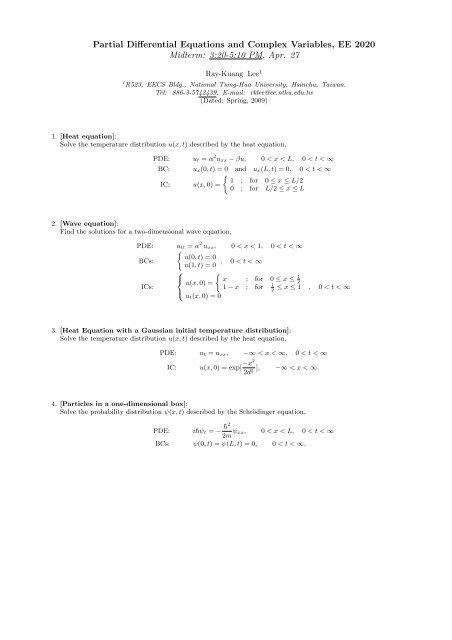
Partial Differential Equations and Complex Variables, EE 2020 ...

Partial Differential Equations and Complex Variables, EE 2020
Midterm: 3:20-5:10 PM, Apr. 27
Ray-Kuang Lee 1
1 R523, EECS Bldg., National Tsing-Hua University, Hsinchu, Taiwan.
Tel: 886-3-5742439, E-mail: rklee@ee.nthu.edu.tw
(Dated: Spring, 2009)
1. [Heat equation]:
Solve the temperature distribution u(x, t) described by the heat equation,
2. [Wave equation]:
Find the solutions for a two-dimensional wave equation,
PDE: ut = α 2 uxx − βu, 0 < x < L, 0 < t < ∞
BC: ux(0, t) = 0 and ux(L, t) = 0, 0 < t < ∞
1 ; for 0 ≤ x ≤ L/2
IC: u(x, 0) =
0 ; for L/2 ≤ x ≤ L
PDE: utt = α 2 uxx, 0 < x < 1, 0 < t < ∞
u(0, t) = 0
BCs:
, 0 < t < ∞
u(1, t) = 0
⎧
1
⎨
x ; for 0 ≤ x ≤
u(x, 0) =
2
1
ICs:
1 − x ; for ≤ x ≤ 1
2 ⎩
ut(x, 0) = 0
3. [Heat Equation with a Gaussian initial temperature distribution]:
Solve the temperature distribution u(x, t) described by the heat equation,
PDE: ut = uxx, −∞ < x < ∞, 0 < t < ∞
IC: u(x, 0) = exp[ −x2
], −∞ < x < ∞.
2d2 4. [Particles in a one-dimensional box]:
Solve the probability distribution ψ(x, t) described by the Schrödinger equation,
, 0 < t < ∞
PDE: i¯hψt = − ¯h2
ψxx,
2m
0 < x < L, 0 < t < ∞
BCs: ψ(0, t) = ψ(L, t) = 0, 0 < t < ∞.

5. [Useful identities and transformations]:
• Finite Sine and Cosine transforms:
• Fourier transform
• Laplace transform
• Hankel transform (Fourier-Bessel)
• Finite Sine transform
• Finite Cosine transform
• Integral identities
• Trigonometry identities
Fs(f) ≡ Fs(ω) = 2
∞
f(t) Sin(ωt)dt,
π 0
Fc(f) ≡ Fc(ω) = 2
∞
f(t) Cos(ωt)dt,
π
F (ω) =
f(t) =
F (s) =
0
1
∞
√
2π
1
√ 2π
∞
0
f(t) = 1
2πi
f(t) e
−∞
−iωt dt,
∞
F (ω) e
−∞
iωt dω,
f(t) e −s t dt,
c+i∞
c−i∞
F (s) e st ds,
∞
Fn(ξ) = r Jn(ξr) f(r)dr,
0
∞
f(r) = Jn(ξr) Fn(ξ)dξ,
n=1
0
L
S [f] = Sn = 2
L 0
f(x) Sin( nπ
L x)dx,
f(x) =
∞
Sn Sin( nπ
L x).
n=1
L
C [f] = Cn = 2
L 0
f(x) Cos( nπ
L x)dx,
f(x) = C0
2 +
∞
Cn Cos( nπ
L x).
∞
e
−∞
−x2
d x = √ π,
∞
e
−∞
−iωt d t = 2πδ(ω).
Sin(α + β)Sin(α − β) = Sin 2 (α) − Sin 2 (β),
Cos(α + β)Cos(α − β) = Cos 2 (α) − Cos 2 (β),
Sin(2α) = 2Sin(α)Cos(α),
Cos(2α) = Cos 2 (α) − Sin 2 (α).
2