A tutorial on support vector regression - RMIT University

Statistics and Computing 14: 199–222, 2004 

C○ 2004 Kluwer Academic Publishers. Manufactured in The Netherlands. 

A <strong>tutorial</strong> on support vector regression ∗ 

ALEX J. SMOLA and BERNHARD SCHÖLKOPF 

RSISE, Australian National University, Canberra 0200, Australia 

Alex.Smola@anu.edu.au 

Max-Planck-Institut für biologische Kybernetik, 72076 Tübingen, Germany 

Bernhard.Schoelkopf@tuebingen.mpg.de 

Received July 2002 and accepted November 2003 

In this <strong>tutorial</strong> we give an overview of the basic ideas underlying Support Vector (SV) machines for 

function estimation. Furthermore, we include a summary of currently used algorithms for training 

SV machines, covering both the quadratic (or convex) programming part and advanced methods for 

dealing with large datasets. Finally, we mention some modifications and extensions that have been 

applied to the standard SV algorithm, and discuss the aspect of regularization from a SV perspective. 

Keywords: machine learning, support vector machines, regression estimation 

1. Introduction 

The purpose of this paper is twofold. It should serve as a selfcontained 

introduction to Support Vector regression for readers 

new to this rapidly developing field of research. 1 On the other 

hand, it attempts to give an overview of recent developments in 

the field. 

To this end, we decided to organize the essay as follows. 

We start by giving a brief overview of the basic techniques in 

Sections 1, 2 and 3, plus a short summary with a number of 

figures and diagrams in Section 4. Section 5 reviews current 

algorithmic techniques used for actually implementing SV 

machines. This may be of most interest for practitioners. 

The following section covers more advanced topics such as 

extensions of the basic SV algorithm, connections between SV 

machines and regularization and briefly mentions methods for 

carrying out model selection. We conclude with a discussion 

of open questions and problems and current directions of SV 

research. Most of the results presented in this review paper 

already have been published elsewhere, but the comprehensive 

presentations and some details are new. 

1.1. Historic background 

The SV algorithm is a nonlinear generalization of the Generalized 

Portrait algorithm developed in Russia in the sixties 2 

∗ An extended version of this paper is available as NeuroCOLT Technical Report 

TR-98-030. 

0960-3174 C○ 2004 Kluwer Academic Publishers 

(Vapnik and Lerner 1963, Vapnik and Chervonenkis 1964). As 

such, it is firmly grounded in the framework of statistical learning 

theory, or VC theory, which has been developed over the last 

three decades by Vapnik and Chervonenkis (1974) and Vapnik 

(1982, 1995). In a nutshell, VC theory characterizes properties 

of learning machines which enable them to generalize well to 

unseen data. 

In its present form, the SV machine was largely developed 

at AT&T Bell Laboratories by Vapnik and co-workers (Boser, 

Guyon and Vapnik 1992, Guyon, Boser and Vapnik 1993, Cortes 

and Vapnik, 1995, Schölkopf, Burges and Vapnik 1995, 1996, 

Vapnik, Golowich and Smola 1997). Due to this industrial context, 

SV research has up to date had a sound orientation towards 

real-world applications. Initial work focused on OCR (optical 

character recognition). Within a short period of time, SV classifiers 

became competitive with the best available systems for 

both OCR and object recognition tasks (Schölkopf, Burges and 

Vapnik 1996, 1998a, Blanz et al. 1996, Schölkopf 1997). A 

comprehensive <strong>tutorial</strong> on SV classifiers has been published by 

Burges (1998). But also in regression and time series prediction 

applications, excellent performances were soon obtained 

(Müller et al. 1997, Drucker et al. 1997, Stitson et al. 1999, 

Mattera and Haykin 1999). A snapshot of the state of the art 

in SV learning was recently taken at the annual Neural Information 

Processing Systems conference (Schölkopf, Burges, 

and Smola 1999a). SV learning has now evolved into an active 

area of research. Moreover, it is in the process of entering the 

standard methods toolbox of machine learning (Haykin 1998, 

Cherkassky and Mulier 1998, Hearst et al. 1998). Schölkopf and

200 Smola and Schölkopf 

Smola (2002) contains a more in-depth overview of SVM regression. 

Additionally, Cristianini and Shawe-Taylor (2000) and Herbrich 

(2002) provide further details on kernels in the context of 

classification. 

1.2. The basic idea 

Suppose we are given training data {(x1, y1), . . . , (xℓ, yℓ)} ⊂ 

X × R, where X denotes the space of the input patterns (e.g. 

X = R d ). These might be, for instance, exchange rates for some 

currency measured at subsequent days together with corresponding 

econometric indicators. In ε-SV regression (Vapnik 1995), 

our goal is to find a function f (x) that has at most ε deviation 

from the actually obtained targets yi for all the training data, and 

at the same time is as flat as possible. In other words, we do not 

care about errors as long as they are less than ε, but will not 

accept any deviation larger than this. This may be important if 

you want to be sure not to lose more than ε money when dealing 

with exchange rates, for instance. 

For pedagogical reasons, we begin by describing the case of 

linear functions f , taking the form 

f (x) = 〈w, x〉 + b with w ∈ X , b ∈ R (1) 

where 〈 · , · 〉 denotes the dot product in X . Flatness in the case 

of (1) means that one seeks a small w. One way to ensure this is 

to minimize the norm, 3 i.e. w 2 = 〈w, w〉. We can write this 

problem as a convex optimization problem: 

minimize 

subject to 

1 

2w2 yi − 〈w, xi〉 − b ≤ ε 

〈w, xi〉 + b − yi ≤ ε 

The tacit assumption in (2) was that such a function f actually 

exists that approximates all pairs (xi, yi) with ε precision, or in 

other words, that the convex optimization problem is feasible. 

Sometimes, however, this may not be the case, or we also may 

want to allow for some errors. Analogously to the “soft margin” 

loss function (Bennett and Mangasarian 1992) which was 

used in SV machines by Cortes and Vapnik (1995), one can introduce 

slack variables ξi, ξ ∗ 

i to cope with otherwise infeasible 

constraints of the optimization problem (2). Hence we arrive at 

the formulation stated in Vapnik (1995). 

1 

minimize 

2 w2 ℓ 

+ C (ξi + ξ 

i=1 

∗ 

i ) 

⎧ 

⎪⎨ yi − 〈w, xi〉 − b ≤ ε + ξi 

subject to 〈w, xi〉 + b − yi ≤ ε + ξ 

⎪⎩ 

∗ 

i 

ξi, ξ ∗ 

(3) 

i ≥ 0 

The constant C > 0 determines the trade-off between the flatness 

of f and the amount up to which deviations larger than 

ε are tolerated. This corresponds to dealing with a so called 

ε-insensitive loss function |ξ|ε described by 

 

0 if |ξ| ≤ ε 

|ξ|ε := 

(4) 

|ξ| − ε otherwise. 

(2) 

Fig. 1. The soft margin loss setting for a linear SVM (from Schölkopf 

and Smola, 2002) 

Figure 1 depicts the situation graphically. Only the points outside 

the shaded region contribute to the cost insofar, as the deviations 

are penalized in a linear fashion. It turns out that in most cases 

the optimization problem (3) can be solved more easily in its dual 

formulation. 4 Moreover, as we will see in Section 2, the dual formulation 

provides the key for extending SV machine to nonlinear 

functions. Hence we will use a standard dualization method utilizing 

Lagrange multipliers, as described in e.g. Fletcher (1989). 

1.3. Dual problem and quadratic programs 

The key idea is to construct a Lagrange function from the objective 

function (it will be called the primal objective function 

in the rest of this article) and the corresponding constraints, by 

introducing a dual set of variables. It can be shown that this 

function has a saddle point with respect to the primal and dual 

variables at the solution. For details see e.g. Mangasarian (1969), 

McCormick (1983), and Vanderbei (1997) and the explanations 

in Section 5.2. We proceed as follows: 

ℓ 

ℓ 

L := 1 

2 w2 + C 

− 

− 

i=1 

(ξi + ξ ∗ 

i 

) − 

i=1 

(ηiξi + η ∗ i 

ℓ 

αi(ε + ξi − yi + 〈w, xi〉 + b) 

i=1 

ℓ 

α 

i=1 

∗ i 

ξ ∗ 

i ) 

(ε + ξ ∗ 

i + yi − 〈w, xi〉 − b) (5) 

Here L is the Lagrangian and ηi, η∗ i , αi, α∗ i are Lagrange multipliers. 

Hence the dual variables in (5) have to satisfy positivity 

constraints, i.e. 

α (∗) 

i , η (∗) 

i ≥ 0. (6) 

Note that by α (∗) 

i , we refer to αi and α∗ i . 

It follows from the saddle point condition that the partial 

derivatives of L with respect to the primal variables (w, b, ξi, ξ ∗ 

i ) 

have to vanish for optimality. 

ℓ 

∂bL = (α ∗ i − αi) = 0 (7) 

i=1 

∂w L = w − 

ℓ 

(αi − α ∗ i )xi = 0 (8) 

i=1 

∂ (∗) 

ξ L = C − α 

i 

(∗) 

i − η(∗) 

i = 0 (9)

A <strong>tutorial</strong> on support vector regression 201 

Substituting (7), (8), and (9) into (5) yields the dual optimization 

problem. 

⎧ 

⎪⎨ − 

maximize 

⎪⎩ 

1 

ℓ 

(αi − α 

2 i, j=1 

∗ i )(α j − α ∗ j )〈xi, x j〉 

ℓ 

−ε (αi + α ∗ ℓ 

i ) + yi(αi − α ∗ i ) (10) 

subject to 

i=1 

i=1 

i=1 

ℓ 

(αi − α ∗ i ) = 0 and αi, α ∗ i ∈ [0, C] 

In deriving (10) we already eliminated the dual variables ηi, η∗ i 

= C − 

through condition (9) which can be reformulated as η (∗) 

i 

α (∗) 

i . Equation (8) can be rewritten as follows 

w = 

ℓ 

(αi−α ∗ i )xi, thus f (x) = 

i=1 

ℓ 

(αi−α ∗ i )〈xi, x〉 + b. (11) 

This is the so-called Support Vector expansion, i.e. w can be 

completely described as a linear combination of the training 

patterns xi. In a sense, the complexity of a function’s representation 

by SVs is independent of the dimensionality of the input 

space X , and depends only on the number of SVs. 

Moreover, note that the complete algorithm can be described 

in terms of dot products between the data. Even when evaluating 

f (x) we need not compute w explicitly. These observations 

will come in handy for the formulation of a nonlinear 

extension. 

1.4. Computing b 

So far we neglected the issue of computing b. The latter can be 

done by exploiting the so called Karush–Kuhn–Tucker (KKT) 

conditions (Karush 1939, Kuhn and Tucker 1951). These state 

that at the point of the solution the product between dual variables 

and constraints has to vanish. 

and 

i=1 

αi(ε + ξi − yi + 〈w, xi〉 + b) = 0 

α ∗ i 

(ε + ξ ∗ 

i + yi − 〈w, xi〉 − b) = 0 

(C − αi)ξi = 0 

(C − α ∗ i 

)ξ ∗ 

i 

= 0. 

(12) 

(13) 

This allows us to make several useful conclusions. Firstly only 

samples (xi, yi) with corresponding α (∗) 

i = C lie outside the εinsensitive 

tube. Secondly αiα ∗ i = 0, i.e. there can never be a set 

of dual variables αi, α∗ i which are both simultaneously nonzero. 

This allows us to conclude that 

ε − yi + 〈w, xi〉 + b ≥ 0 and ξi = 0 if αi < C (14) 

ε − yi + 〈w, xi〉 + b ≤ 0 if αi > 0 (15) 

In conjunction with an analogous analysis on α∗ i we have 

max{−ε + yi − 〈w, xi〉 | αi < C or α∗ i > 0} ≤ b ≤ 

min{−ε + yi − 〈w, xi〉 | αi > 0 or α∗ i < C} 

(16) 

If some α (∗) 

i ∈ (0, C) the inequalities become equalities. See 

also Keerthi et al. (2001) for further means of choosing b. 

Another way of computing b will be discussed in the context 

of interior point optimization (cf. Section 5). There b turns out 

to be a by-product of the optimization process. Further considerations 

shall be deferred to the corresponding section. See also 

Keerthi et al. (1999) for further methods to compute the constant 

offset. 

A final note has to be made regarding the sparsity of the SV 

expansion. From (12) it follows that only for | f (xi) − yi| ≥ ε 

the Lagrange multipliers may be nonzero, or in other words, for 

all samples inside the ε–tube (i.e. the shaded region in Fig. 1) 

the αi, α∗ i vanish: for | f (xi) − yi| < ε the second factor in 

(12) is nonzero, hence αi, α ∗ i 

has to be zero such that the KKT 

conditions are satisfied. Therefore we have a sparse expansion 

of w in terms of xi (i.e. we do not need all xi to describe w). The 

examples that come with nonvanishing coefficients are called 

Support Vectors. 

2. Kernels 

2.1. Nonlinearity by preprocessing 

The next step is to make the SV algorithm nonlinear. This, for 

instance, could be achieved by simply preprocessing the training 

patterns xi by a map : X → F into some feature space F, 

as described in Aizerman, Braverman and Rozonoér (1964) and 

Nilsson (1965) and then applying the standard SV regression 

algorithm. Let us have a brief look at an example given in Vapnik 

(1995). 

Example 1 (Quadratic features in R2 ). Consider the map : 

R2 → R3 with (x1, x2) = (x 2 1 , √ 2x1x2, x 2 2 ). It is understood 

that the subscripts in this case refer to the components of x ∈ R2 . 

Training a linear SV machine on the preprocessed features would 

yield a quadratic function. 

While this approach seems reasonable in the particular example 

above, it can easily become computationally infeasible 

for both polynomial features of higher order and higher dimensionality, 

as the number of different monomial features 

of degree p is ( d+p−1 

p ), where d = dim(X ). Typical values 

for OCR tasks (with good performance) (Schölkopf, Burges 

and Vapnik 1995, Schölkopf et al. 1997, Vapnik 1995) are 

p = 7, d = 28 · 28 = 784, corresponding to approximately 

3.7 · 1016 features. 

2.2. Implicit mapping via kernels 

Clearly this approach is not feasible and we have to find a computationally 

cheaper way. The key observation (Boser, Guyon


and Vapnik 1992) is that for the feature map of example 2.1 we 

have 

2 

x1 , √ 2x1x2, x 2 ′2 

2 , x 1 , √ 2x ′ 1x ′ 2, x ′2 

′ 2 

2 = 〈x, x 〉 . (17) 

As noted in the previous section, the SV algorithm only depends 

on dot products between patterns xi. Hence it suffices to know 

k(x, x ′ ) := 〈(x), (x ′ )〉 rather than explicitly which allows 

us to restate the SV optimization problem: 

maximize 

subject to 

⎧ 

⎪⎨ 

− 1 

2 

⎪⎩ −ε 

i=1 

ℓ 

(αi − α ∗ i )(α j − α ∗ j )k(xi, x j) 

i, j=1 

ℓ 

(αi + α ∗ i ) + 

i=1 

ℓ 

yi(αi − α ∗ i ) 

i=1 

ℓ 

(αi − α ∗ i ) = 0 and αi, α ∗ i ∈ [0, C] 

Likewise the expansion of f (11) may be written as 

ℓ 

w = (αi − α ∗ i )(xi) and 

f (x) = 

i=1 

(18) 

ℓ 

(αi − α ∗ i )k(xi, x) + b. (19) 

i=1 

The difference to the linear case is that w is no longer given explicitly. 

Also note that in the nonlinear setting, the optimization 

problem corresponds to finding the flattest function in feature 

space, not in input space. 

2.3. Conditions for kernels 

The question that arises now is, which functions k(x, x ′ ) correspond 

to a dot product in some feature space F. The following 

theorem characterizes these functions (defined on X ). 

Theorem 2 (Mercer 1909). Suppose k ∈ L∞(X 2 ) such that 

the integral operator Tk : L2(X ) → L2(X ), 

 

Tk f (·) := k(·, x) f (x)dµ(x) (20) 

X 

is positive (here µ denotes a measure on X with µ(X ) finite 

and supp(µ) = X ). Let ψ j ∈ L2(X ) be the eigenfunction of Tk 

associated with the eigenvalue λ j = 0 and normalized such that 

ψ jL2 = 1 and let ψ j denote its complex conjugate. Then 

1. (λ j(T )) j ∈ ℓ1. 

2. k(x, x ′ ) = 

j∈N λ jψj(x)ψ j(x ′ ) holds for almost all (x, x ′ ), 

where the series converges absolutely and uniformly for almost 

all (x, x ′ ). 

Less formally speaking this theorem means that if 

 

k(x, x ′ ) f (x) f (x ′ ) dxdx ′ ≥ 0 for all f ∈ L2(X ) (21) 

X ×X 

holds we can write k(x, x ′ ) as a dot product in some feature 

space. From this condition we can conclude some simple rules 

for compositions of kernels, which then also satisfy Mercer’s 

condition (Schölkopf, Burges and Smola 1999a). In the following 

we will call such functions k admissible SV kernels. 

Corollary 3 (Positive linear combinations of kernels). Denote 

by k1, k2 admissible SV kernels and c1, c2 ≥ 0 then 

k(x, x ′ ) := c1k1(x, x ′ ) + c2k2(x, x ′ ) (22) 

is an admissible kernel. This follows directly from (21) by virtue 

of the linearity of integrals. 

More generally, one can show that the set of admissible kernels 

forms a convex cone, closed in the topology of pointwise 

convergence (Berg, Christensen and Ressel 1984). 

Corollary 4 (Integrals of kernels). Let s(x, x ′ ) be a function 

on X × X such that 

k(x, x ′ 

) := s(x, z)s(x ′ , z) dz (23) 

exists. Then k is an admissible SV kernel. 

X 

This can be shown directly from (21) and (23) by rearranging the 

order of integration. We now state a necessary and sufficient condition 

for translation invariant kernels, i.e. k(x, x ′ ) := k(x − x ′ ) 

as derived in Smola, Schölkopf and Müller (1998c). 

Theorem 5 (Products of kernels). Denote by k1 and k2 admissible 

SV kernels then 

is an admissible kernel. 

k(x, x ′ ) := k1(x, x ′ )k2(x, x ′ ) (24) 

This can be seen by an application of the “expansion part” of 

Mercer’s theorem to the kernels k1 and k2 and observing that 

each term in the double sum 

i, j λ1 i λ2 j ψ 1 i (x)ψ 1 i (x ′ )ψ 2 j (x)ψ 2 j (x ′ ) 

gives rise to a positive coefficient when checking (21). 

Theorem 6 (Smola, Schölkopf and Müller 1998c). A translation 

invariant kernel k(x, x ′ ) = k(x − x ′ ) is an admissible SV 

kernels if and only if the Fourier transform 

 

d 

− 

F[k](ω) = (2π) 2 e −i〈ω,x〉 k(x)dx (25) 

is nonnegative. 

We will give a proof and some additional explanations to this 

theorem in Section 7. It follows from interpolation theory 

(Micchelli 1986) and the theory of regularization networks 

(Girosi, Jones and Poggio 1993). For kernels of the dot-product 

type, i.e. k(x, x ′ ) = k(〈x, x ′ 〉), there exist sufficient conditions 

for being admissible. 

Theorem 7 (Burges 1999). Any kernel of dot-product type 

k(x, x ′ ) = k(〈x, x ′ 〉) has to satisfy 

X 

k(ξ) ≥ 0, ∂ξ k(ξ) ≥ 0 and ∂ξ k(ξ) + ξ∂ 2 ξ k(ξ) ≥ 0 (26) 

for any ξ ≥ 0 in order to be an admissible SV kernel.


Note that the conditions in Theorem 7 are only necessary but 

not sufficient. The rules stated above can be useful tools for 

practitioners both for checking whether a kernel is an admissible 

SV kernel and for actually constructing new kernels. The general 

case is given by the following theorem. 

Theorem 8 (Schoenberg 1942). A kernel of dot-product type 

k(x, x ′ ) = k(〈x, x ′ 〉) defined on an infinite dimensional Hilbert 

space, with a power series expansion 

∞ 

k(t) = ant n 

(27) 

n=0 

is admissible if and only if all an ≥ 0. 

A slightly weaker condition applies for finite dimensional 

spaces. For further details see Berg, Christensen and Ressel 

(1984) and Smola, Óvári and Williamson (2001). 

2.4. Examples 

In Schölkopf, Smola and Müller (1998b) it has been shown, by 

explicitly computing the mapping, that homogeneous polynomial 

kernels k with p ∈ N and 

k(x, x ′ ) = 〈x, x ′ 〉 p 

(28) 

are suitable SV kernels (cf. Poggio 1975). From this observation 

one can conclude immediately (Boser, Guyon and Vapnik 1992, 

Vapnik 1995) that kernels of the type 

k(x, x ′ ) = (〈x, x ′ 〉 + c) p 

(29) 

i.e. inhomogeneous polynomial kernels with p ∈ N, c ≥ 0 are 

admissible, too: rewrite k as a sum of homogeneous kernels and 

apply Corollary 3. Another kernel, that might seem appealing 

due to its resemblance to Neural Networks is the hyperbolic 

tangent kernel 

k(x, x ′ ) = tanh(ϑ + κ〈x, x ′ 〉). (30) 

By applying Theorem 8 one can check that this kernel does 

not actually satisfy Mercer’s condition (Ovari 2000). Curiously, 

the kernel has been successfully used in practice; cf. Scholkopf 

(1997) for a discussion of the reasons. 

Translation invariant kernels k(x, x ′ ) = k(x − x ′ ) are 

quite widespread. It was shown in Aizerman, Braverman and 

Rozonoér (1964), Micchelli (1986) and Boser, Guyon and Vapnik 

(1992) that 

k(x, x ′ ) = e − x−x′ 2 

2σ 2 (31) 

is an admissible SV kernel. Moreover one can show (Smola 

1996, Vapnik, Golowich and Smola 1997) that (1X denotes the 

indicator function on the set X and ⊗ the convolution operation) 

k(x, x ′ ) = B2n+1(x − x ′ ) with Bk := 

k 

i=1 

1 1 1 

[− 2 , 2] 

(32) 

B-splines of order 2n + 1, defined by the 2n + 1 convolution of 

the unit inverval, are also admissible. We shall postpone further 

considerations to Section 7 where the connection to regularization 

operators will be pointed out in more detail. 

3. Cost functions 

So far the SV algorithm for regression may seem rather strange 

and hardly related to other existing methods of function estimation 

(e.g. Huber 1981, Stone 1985, Härdle 1990, Hastie and 

Tibshirani 1990, Wahba 1990). However, once cast into a more 

standard mathematical notation, we will observe the connections 

to previous work. For the sake of simplicity we will, again, 

only consider the linear case, as extensions to the nonlinear one 

are straightforward by using the kernel method described in the 

previous chapter. 

3.1. The risk functional 

Let us for a moment go back to the case of Section 1.2. There, we 

had some training data X := {(x1, y1), . . . , (xℓ, yℓ)} ⊂ X × R. 

We will assume now, that this training set has been drawn iid 

(independent and identically distributed) from some probability 

distribution P(x, y). Our goal will be to find a function f 

minimizing the expected risk (cf. Vapnik 1982) 

 

R[ f ] = c(x, y, f (x))d P(x, y) (33) 

(c(x, y, f (x)) denotes a cost function determining how we will 

penalize estimation errors) based on the empirical data X. Given 

that we do not know the distribution P(x, y) we can only use 

X for estimating a function f that minimizes R[ f ]. A possible 

approximation consists in replacing the integration by the 

empirical estimate, to get the so called empirical risk functional 

Remp[ f ] := 1 

ℓ 

ℓ 

c(xi, yi, f (xi)). (34) 

i=1 

A first attempt would be to find the empirical risk minimizer 

f0 := argmin f ∈H Remp[ f ] for some function class H. However, 

if H is very rich, i.e. its “capacity” is very high, as for instance 

when dealing with few data in very high-dimensional spaces, 

this may not be a good idea, as it will lead to overfitting and thus 

bad generalization properties. Hence one should add a capacity 

control term, in the SV case w 2 , which leads to the regularized 

risk functional (Tikhonov and Arsenin 1977, Morozov 1984, 

Vapnik 1982) 

Rreg[ f ] := Remp[ f ] + λ 

2 w2 

(35) 

where λ > 0 is a so called regularization constant. Many 

algorithms like regularization networks (Girosi, Jones and 

Poggio 1993) or neural networks with weight decay networks 

(e.g. Bishop 1995) minimize an expression similar to (35).


3.2. Maximum likelihood and density models 

The standard setting in the SV case is, as already mentioned in 

Section 1.2, the ε-insensitive loss 

c(x, y, f (x)) = |y − f (x)|ε. (36) 

It is straightforward to show that minimizing (35) with the particular 

loss function of (36) is equivalent to minimizing (3), the 

only difference being that C = 1/(λℓ). 

Loss functions such like |y − f (x)| p ε with p > 1 may not 

be desirable, as the superlinear increase leads to a loss of the 

robustness properties of the estimator (Huber 1981): in those 

cases the derivative of the cost function grows without bound. 

For p < 1, on the other hand, c becomes nonconvex. 

For the case of c(x, y, f (x)) = (y − f (x)) 2 we recover the 

least mean squares fit approach, which, unlike the standard SV 

loss function, leads to a matrix inversion instead of a quadratic 

programming problem. 

The question is which cost function should be used in (35). On 

the one hand we will want to avoid a very complicated function c 

as this may lead to difficult optimization problems. On the other 

hand one should use that particular cost function that suits the 

problem best. Moreover, under the assumption that the samples 

were generated by an underlying functional dependency plus 

additive noise, i.e. yi = ftrue(xi) + ξi with density p(ξ), then the 

optimal cost function in a maximum likelihood sense is 

c(x, y, f (x)) = − log p(y − f (x)). (37) 

This can be seen as follows. The likelihood of an estimate 

X f := {(x1, f (x1)), . . . , (xℓ, f (xℓ))} (38) 

for additive noise and iid data is 

ℓ 

p(X f | X) = p( f (xi) | (xi, yi)) = 

i=1 

ℓ 

p(yi − f (xi)). (39) 

Maximizing P(X f | X) is equivalent to minimizing − log P 

(X f | X). By using (37) we get 

ℓ 

− log P(X f | X) = c(xi, yi, f (xi)). (40) 

Table 1. Common loss functions and corresponding density models 

i=1 

i=1 

However, the cost function resulting from this reasoning might 

be nonconvex. In this case one would have to find a convex 

proxy in order to deal with the situation efficiently (i.e. to find 

an efficient implementation of the corresponding optimization 

problem). 

If, on the other hand, we are given a specific cost function from 

a real world problem, one should try to find as close a proxy to 

this cost function as possible, as it is the performance wrt. this 

particular cost function that matters ultimately. 

Table 1 contains an overview over some common density 

models and the corresponding loss functions as defined by 

(37). 

The only requirement we will impose on c(x, y, f (x)) in the 

following is that for fixed x and y we have convexity in f (x). 

This requirement is made, as we want to ensure the existence and 

uniqueness (for strict convexity) of a minimum of optimization 

problems (Fletcher 1989). 

3.3. Solving the equations 

For the sake of simplicity we will additionally assume c to 

be symmetric and to have (at most) two (for symmetry) discontinuities 

at ±ε, ε ≥ 0 in the first derivative, and to be 

zero in the interval [−ε, ε]. All loss functions from Table 1 

belong to this class. Hence c will take on the following 

form. 

c(x, y, f (x)) = ˜c(|y − f (x)|ε) (41) 

Note the similarity to Vapnik’s ε-insensitive loss. It is rather 

straightforward to extend this special choice to more general 

convex cost functions. For nonzero cost functions in the interval 

[−ε, ε] use an additional pair of slack variables. Moreover 

and different 

we might choose different cost functions ˜ci, ˜c ∗ i 

values of εi, ε ∗ i 

Loss function Density model 

for each sample. At the expense of additional 

Lagrange multipliers in the dual formulation additional discontinuities 

also can be taken care of. Analogously to (3) we arrive at 

a convex minimization problem (Smola and Schölkopf 1998a). 

To simplify notation we will stick to the one of (3) and use C 

ε-insensitive c(ξ) = |ξ|ε p(ξ) = 1 

2(1+ε) exp(−|ξ|ε) 

Laplacian c(ξ) = |ξ| p(ξ) = 1 

2 exp(−|ξ|) 

 

Gaussian c(ξ) = 1 

2 ξ 2 p(ξ) = 1 

Huber’s robust loss 

 

1 

2σ 

c(ξ) = 

√ exp − 

2π 2 

(ξ)2 |ξ| − 

if |ξ| ≤ σ 

σ 

2 otherwise 

⎧ 

⎨ 

ξ 2 

exp − 2σ 

p(ξ) ∝ 

⎩ σ 

exp − |ξ| 2 

if |ξ| ≤ σ 

otherwise 

Polynomial c(ξ) = 1 

p |ξ|p p(ξ) = p 

2Ɣ(1/p) exp(−|ξ|p Piecewise polynomial 

 

1 

pσ 

c(ξ) = 

) 

p−1 (ξ) p |ξ| − σ 

if |ξ| ≤ σ 

p−1 

p otherwise 

⎧ 

⎨ 

ξ p 

exp − pσ 

p(ξ) ∝ 

⎩ 

p−1 

 

 

exp − |ξ| 

if |ξ| ≤ σ 

otherwise 

σ p−1 

p 

ξ 2


instead of normalizing by λ and ℓ. 

minimize 

subject to 

1 

2 w2 ℓ 

+ C ( ˜c(ξi) + ˜c(ξ 

i=1 

∗ 

i )) 

⎧ 

⎪⎨ yi − 〈w, xi〉 − b ≤ ε + ξi 

〈w, xi〉 + b − yi ≤ ε + ξ 

⎪⎩ 

∗ 

i 

ξi, ξ ∗ 

i 

≥ 0 

(42) 

Again, by standard Lagrange multiplier techniques, exactly in 

the same manner as in the |·|ε case, one can compute the dual optimization 

problem (the main difference is that the slack variable 

terms ˜c(ξ (∗) 

i ) now have nonvanishing derivatives). We will omit 

the indices i and ∗ , where applicable to avoid tedious notation. 

This yields 

maximize 

⎧ 

− 

⎪⎨ 

1 

ℓ 

(αi − α 

2 i, j=1 

∗ i )(α j − α ∗ j )〈xi, x j〉 

ℓ 

+ yi(αi − α ∗ i ) − ε(αi + α ∗ i ) 

⎪⎩ +C 

i=1 

ℓ 

i=1 

T (ξi) + T (ξ ∗ 

i ) 

⎧ 

⎪⎨ 

ℓ 

w = (αi − α 

where 

⎪⎩ 

i=1 

∗ i )xi 

T (ξ) := ˜c(ξ) − ξ∂ξ ˜c(ξ) 

⎧ 

ℓ 

(αi − α 

⎪⎨ i=1 

subject to 

∗ i ) = 0 

α ≤ C∂ξ ˜c(ξ) 

3.4. Examples 

ξ = inf{ξ | C∂ξ ˜c ≥ α} 

⎪⎩ 

α, ξ ≥ 0 

(43) 

Let us consider the examples of Table 1. We will show explicitly 

for two examples how (43) can be further simplified to bring it 

into a form that is practically useful. In the ε-insensitive case, 

i.e. ˜c(ξ) = |ξ| we get 

T (ξ) = ξ − ξ · 1 = 0. (44) 

Morover one can conclude from ∂ξ ˜c(ξ) = 1 that 

ξ = inf{ξ | C ≥ α} = 0 and α ∈ [0, C]. (45) 

For the case of piecewise polynomial loss we have to distinguish 

two different cases: ξ ≤ σ and ξ > σ . In the first case we get 

T (ξ) = 

1 

pσ p−1 ξ p − 1 

σ p−1 ξ p p − 1 

= − 

p σ 1−p ξ p 

and ξ = inf{ξ | Cσ 1−pξ p−1 1 

− 

≥ α} = σ C p−1 α 1 

p−1 and thus 

T (ξ) = − 

(46) 

p − 1 

p 

σ C− p−1 α 

p p 

p−1 . (47) 

Table 2. Terms of the convex optimization problem depending on the 

choice of the loss function 

ε α CT (α) 

ε-insensitive ε = 0 α ∈ [0, C] 0 

Laplacian ε = 0 α ∈ [0, C] 0 

Gaussian ε = 0 α ∈ [0, ∞) − 1 

2 C −1 α 2 

Huber’s ε = 0 α ∈ [0, C] − 1 

2 σ C −1 α 2 

robust loss 

Polynomial ε = 0 α ∈ [0, ∞) − p−1 − 

1 

C p−1 α p p 

p−1 

Piecewise ε = 0 α ∈ [0, C] − p−1 

p 

polynomial 

In the second case (ξ ≥ σ ) we have 

T (ξ) = ξ − σ 

p − 1 

p 

− ξ = −σ p − 1 

p 

σ C − 1 

p−1 α p 

p−1 

(48) 

and ξ = inf{ξ | C ≥ α} = σ , which, in turn yields α ∈ [0, C]. 

Combining both cases we have 

p − 1 

p 

α ∈ [0, C] and T (α) = − σ C− p−1 α 

p p 

p−1 . (49) 

Table 2 contains a summary of the various conditions on α and 

formulas for T (α) (strictly speaking T (ξ(α))) for different cost 

functions. 5 Note that the maximum slope of ˜c determines the 

region of feasibility of α, i.e. s := sup ξ∈R + ∂ξ ˜c(ξ) < ∞ leads to 

compact intervals [0, Cs] for α. This means that the influence 

of a single pattern is bounded, leading to robust estimators 

(Huber 1972). One can also observe experimentally that the 

performance of a SV machine depends significantly on the cost 

function used (Müller et al. 1997, Smola, Schölkopf and Müller 

1998b) 

A cautionary remark is necessary regarding the use of cost 

functions other than the ε-insensitive one. Unless ε = 0 we 

will lose the advantage of a sparse decomposition. This may 

be acceptable in the case of few data, but will render the prediction 

step extremely slow otherwise. Hence one will have to 

trade off a potential loss in prediction accuracy with faster predictions. 

Note, however, that also a reduced set algorithm like 

in Burges (1996), Burges and Schölkopf (1997) and Schölkopf 

et al. (1999b) or sparse decomposition techniques (Smola and 

Schölkopf 2000) could be applied to address this issue. In a 

Bayesian setting, Tipping (2000) has recently shown how an L2 

cost function can be used without sacrificing sparsity. 

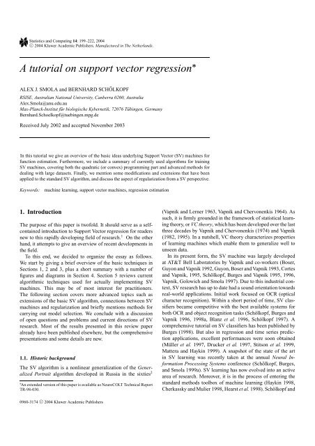
4. The bigger picture 

Before delving into algorithmic details of the implementation 

let us briefly review the basic properties of the SV algorithm 

for regression as described so far. Figure 2 contains a graphical 

overview over the different steps in the regression stage. 

The input pattern (for which a prediction is to be made) is 

mapped into feature space by a map . Then dot products 

are computed with the images of the training patterns under


Fig. 2. Architecture of a regression machine constructed by the SV 

algorithm 

the map . This corresponds to evaluating kernel functions 

k(xi, x). Finally the dot products are added up using the weights 

νi = αi − α∗ i . This, plus the constant term b yields the final 

prediction output. The process described here is very similar to 

regression in a neural network, with the difference, that in the 

SV case the weights in the input layer are a subset of the training 

patterns. 

Figure 3 demonstrates how the SV algorithm chooses the 

flattest function among those approximating the original data 

with a given precision. Although requiring flatness only in 

feature space, one can observe that the functions also are 

very flat in input space. This is due to the fact, that kernels 

can be associated with flatness properties via regular- 

ization operators. This will be explained in more detail in 

Section 7. 

Finally Fig. 4 shows the relation between approximation quality 

and sparsity of representation in the SV case. The lower the 

precision required for approximating the original data, the fewer 

SVs are needed to encode that. The non-SVs are redundant, i.e. 

even without these patterns in the training set, the SV machine 

would have constructed exactly the same function f . One might 

think that this could be an efficient way of data compression, 

namely by storing only the support patterns, from which the estimate 

can be reconstructed completely. However, this simple 

analogy turns out to fail in the case of high-dimensional data, 

and even more drastically in the presence of noise. In Vapnik, 

Golowich and Smola (1997) one can see that even for moderate 

approximation quality, the number of SVs can be considerably 

high, yielding rates worse than the Nyquist rate (Nyquist 1928, 

Shannon 1948). 

5. Optimization algorithms 

While there has been a large number of implementations of SV 

algorithms in the past years, we focus on a few algorithms which 

will be presented in greater detail. This selection is somewhat 

biased, as it contains these algorithms the authors are most familiar 

with. However, we think that this overview contains some 

of the most effective ones and will be useful for practitioners 

who would like to actually code a SV machine by themselves. 

But before doing so we will briefly cover major optimization 

packages and strategies. 

Fig. 3. Left to right: approximation of the function sinc x with precisions ε = 0.1, 0.2, and 0.5. The solid top and the bottom lines indicate the size 

of the ε-tube, the dotted line in between is the regression 

Fig. 4. Left to right: regression (solid line), datapoints (small dots) and SVs (big dots) for an approximation with ε = 0.1, 0.2, and 0.5. Note the 

decrease in the number of SVs


5.1. Implementations 

Most commercially available packages for quadratic programming 

can also be used to train SV machines. These are usually 

numerically very stable general purpose codes, with special enhancements 

for large sparse systems. While the latter is a feature 

that is not needed at all in SV problems (there the dot product 

matrix is dense and huge) they still can be used with good success. 

6 

OSL: This package was written by IBM-Corporation (1992). It 

uses a two phase algorithm. The first step consists of solving 

a linear approximation of the QP problem by the simplex algorithm 

(Dantzig 1962). Next a related very simple QP problem 

is dealt with. When successive approximations are close 

enough together, the second subalgorithm, which permits a 

quadratic objective and converges very rapidly from a good 

starting value, is used. Recently an interior point algorithm 

was added to the software suite. 

CPLEX by CPLEX-Optimization-Inc. (1994) uses a primal-dual 

logarithmic barrier algorithm (Megiddo 1989) instead with 

predictor-corrector step (see e.g. Lustig, Marsten and Shanno 

1992, Mehrotra and Sun 1992). 

MINOS by the Stanford Optimization Laboratory (Murtagh and 

Saunders 1983) uses a reduced gradient algorithm in conjunction 

with a quasi-Newton algorithm. The constraints are 

handled by an active set strategy. Feasibility is maintained 

throughout the process. On the active constraint manifold, a 

quasi-Newton approximation is used. 

MATLAB: Until recently the matlab QP optimizer delivered only 

agreeable, although below average performance on classification 

tasks and was not all too useful for regression tasks 

(for problems much larger than 100 samples) due to the fact 

that one is effectively dealing with an optimization problem 

of size 2ℓ where at least half of the eigenvalues of the 

Hessian vanish. These problems seem to have been addressed 

in version 5.3 / R11. Matlab now uses interior point codes. 

LOQO by Vanderbei (1994) is another example of an interior 

point code. Section 5.3 discusses the underlying strategies in 

detail and shows how they can be adapted to SV algorithms. 

Maximum margin perceptron by Kowalczyk (2000) is an algorithm 

specifically tailored to SVs. Unlike most other techniques 

it works directly in primal space and thus does not 

have to take the equality constraint on the Lagrange multipliers 

into account explicitly. 

Iterative free set methods The algorithm by Kaufman (Bunch, 

Kaufman and Parlett 1976, Bunch and Kaufman 1977, 1980, 

Drucker et al. 1997, Kaufman 1999), uses such a technique 

starting with all variables on the boundary and adding them as 

the Karush Kuhn Tucker conditions become more violated. 

This approach has the advantage of not having to compute 

the full dot product matrix from the beginning. Instead it is 

evaluated on the fly, yielding a performance improvement 

in comparison to tackling the whole optimization problem 

at once. However, also other algorithms can be modified by 

subset selection techniques (see Section 5.5) to address this 

problem. 

5.2. Basic notions 

Most algorithms rely on results from the duality theory in convex 

optimization. Although we already happened to mention some 

basic ideas in Section 1.2 we will, for the sake of convenience, 

briefly review without proof the core results. These are needed 

in particular to derive an interior point algorithm. For details and 

proofs (see e.g. Fletcher 1989). 

Uniqueness: Every convex constrained optimization problem 

has a unique minimum. If the problem is strictly convex then 

the solution is unique. This means that SVs are not plagued 

with the problem of local minima as Neural Networks are. 7 

Lagrange function: The Lagrange function is given by the primal 

objective function minus the sum of all products between 

constraints and corresponding Lagrange multipliers (cf. e.g. 

Fletcher 1989, Bertsekas 1995). Optimization can be seen 

as minimzation of the Lagrangian wrt. the primal variables 

and simultaneous maximization wrt. the Lagrange multipliers, 

i.e. dual variables. It has a saddle point at the solution. 

Usually the Lagrange function is only a theoretical device to 

derive the dual objective function (cf. Section 1.2). 

Dual objective function: It is derived by minimizing the 

Lagrange function with respect to the primal variables and 

subsequent elimination of the latter. Hence it can be written 

solely in terms of the dual variables. 

Duality gap: For both feasible primal and dual variables the primal 

objective function (of a convex minimization problem) 

is always greater or equal than the dual objective function. 

Since SVMs have only linear constraints the constraint qualifications 

of the strong duality theorem (Bazaraa, Sherali and 

Shetty 1993, Theorem 6.2.4) are satisfied and it follows that 

gap vanishes at optimality. Thus the duality gap is a measure 

how close (in terms of the objective function) the current set 

of variables is to the solution. 

Karush–Kuhn–Tucker (KKT) conditions: A set of primal and 

dual variables that is both feasible and satisfies the KKT 

conditions is the solution (i.e. constraint · dual variable = 0). 

The sum of the violated KKT terms determines exactly the 

size of the duality gap (that is, we simply compute the 

constraint · Lagrangemultiplier part as done in (55)). This 

allows us to compute the latter quite easily. 

A simple intuition is that for violated constraints the dual 

variable could be increased arbitrarily, thus rendering the 

Lagrange function arbitrarily large. This, however, is in contradition 

to the saddlepoint property. 

5.3. Interior point algorithms 

In a nutshell the idea of an interior point algorithm is to compute 

the dual of the optimization problem (in our case the dual 

dual of Rreg[ f ]) and solve both primal and dual simultaneously. 

This is done by only gradually enforcing the KKT conditions


to iteratively find a feasible solution and to use the duality 

gap between primal and dual objective function to determine 

the quality of the current set of variables. The special flavour 

of algorithm we will describe is primal-dual path-following 

(Vanderbei 1994). 

In order to avoid tedious notation we will consider the slightly 

more general problem and specialize the result to the SVM later. 

It is understood that unless stated otherwise, variables like α 

denote vectors and αi denotes its i-th component. 

1 

minimize q(α) + 〈c, α〉 

2 (50) 

subject to Aα = b and l ≤ α ≤ u 

with c, α, l, u ∈ Rn , A ∈ Rn·m , b ∈ Rm , the inequalities between 

vectors holding componentwise and q(α) being a convex 

function of α. Now we will add slack variables to get rid of all 

inequalities but the positivity constraints. This yields: 

1 

minimize q(α) + 〈c, α〉 

2 

subject to Aα = b, α − g = l, α + t = u, (51) 

The dual of (51) is 

maximize 

subject to 

g, t ≥ 0, α free 

1 

2 (q(α) − 〈∂q(α), α)〉 + 〈b, y〉 + 〈l, z〉 − 〈u, s〉 

1 

2 ∂q(α) + c − (Ay) ⊤ + s = z, s, z ≥ 0, y free 

Moreover we get the KKT conditions, namely 

(52) 

gi zi = 0 and siti = 0 for all i ∈ [1 . . . n]. (53) 

A necessary and sufficient condition for the optimal solution is 

that the primal/dual variables satisfy both the feasibility conditions 

of (51) and (52) and the KKT conditions (53). We proceed 

to solve (51)–(53) iteratively. The details can be found in 

Appendix A. 

5.4. Useful tricks 

Before proceeding to further algorithms for quadratic optimization 

let us briefly mention some useful tricks that can be applied 

to all algorithms described subsequently and may have significant 

impact despite their simplicity. They are in part derived 

from ideas of the interior-point approach. 

Training with different regularization parameters: For several 

reasons (model selection, controlling the number of support 

vectors, etc.) it may happen that one has to train a SV machine 

with different regularization parameters C, but otherwise 

rather identical settings. If the parameters Cnew = τCold 

is not too different it is advantageous to use the rescaled values 

of the Lagrange multipliers (i.e. αi, α∗ i ) as a starting point 

for the new optimization problem. Rescaling is necessary to 

satisfy the modified constraints. One gets 

αnew = ταold and likewise bnew = τbold. (54) 

Assuming that the (dominant) convex part q(α) of the primal 

objective is quadratic, the q scales with τ 2 where as the 

linear part scales with τ. However, since the linear term dominates 

the objective function, the rescaled values are still a 

better starting point than α = 0. In practice a speedup of 

approximately 95% of the overall training time can be observed 

when using the sequential minimization algorithm, 

cf. (Smola 1998). A similar reasoning can be applied when 

retraining with the same regularization parameter but different 

(yet similar) width parameters of the kernel function. See 

Cristianini, Campbell and Shawe-Taylor (1998) for details 

thereon in a different context. 

Monitoring convergence via the feasibility gap: In the case of 

both primal and dual feasible variables the following connection 

between primal and dual objective function holds: 

Dual Obj. = Primal Obj. − 

(gi zi + siti) (55) 

This can be seen immediately by the construction of the 

Lagrange function. In Regression Estimation (with the εinsensitive 

loss function) one obtains for 

i gi zi + siti 

⎡ 

+ max(0, f (xi) − (yi + εi))(C − α 

⎢ 

⎣ 

∗ i ) 

− min(0, f (xi) − (yi + εi))α∗ i 

+ max(0, (yi − ε∗ i ) − f (xi))(C 

⎤ 

⎥ . (56) 

− αi) ⎦ 

i 

− min(0, (yi − ε∗ i ) − f (xi))αi 

Thus convergence with respect to the point of the solution 

can be expressed in terms of the duality gap. An effective 

stopping rule is to require 

 

i gi zi + siti 

≤ εtol (57) 

|Primal Objective| + 1 

for some precision εtol. This condition is much in the spirit of 

primal dual interior point path following algorithms, where 

convergence is measured in terms of the number of significant 

figures (which would be the decimal logarithm of (57)), a 

convention that will also be adopted in the subsequent parts 

of this exposition. 

5.5. Subset selection algorithms 

The convex programming algorithms described so far can be 

used directly on moderately sized (up to 3000) samples datasets 

without any further modifications. On large datasets, however, it 

is difficult, due to memory and cpu limitations, to compute the 

dot product matrix k(xi, x j) and keep it in memory. A simple 

calculation shows that for instance storing the dot product matrix 

of the NIST OCR database (60.000 samples) at single precision 

would consume 0.7 GBytes. A Cholesky decomposition thereof, 

which would additionally require roughly the same amount of 

memory and 64 Teraflops (counting multiplies and adds separately), 

seems unrealistic, at least at current processor speeds. 

A first solution, which was introduced in Vapnik (1982) relies 

on the observation that the solution can be reconstructed from 

the SVs alone. Hence, if we knew the SV set beforehand, and 

i


it fitted into memory, then we could directly solve the reduced 

problem. The catch is that we do not know the SV set before 

solving the problem. The solution is to start with an arbitrary 

subset, a first chunk that fits into memory, train the SV algorithm 

on it, keep the SVs and fill the chunk up with data the current 

estimator would make errors on (i.e. data lying outside the εtube 

of the current regression). Then retrain the system and keep 

on iterating until after training all KKT-conditions are satisfied. 

The basic chunking algorithm just postponed the underlying 

problem of dealing with large datasets whose dot-product matrix 

cannot be kept in memory: it will occur for larger training set 

sizes than originally, but it is not completely avoided. Hence 

the solution is Osuna, Freund and Girosi (1997) to use only a 

subset of the variables as a working set and optimize the problem 

with respect to them while freezing the other variables. This 

method is described in detail in Osuna, Freund and Girosi (1997), 

Joachims (1999) and Saunders et al. (1998) for the case of pattern 

recognition. 8 

An adaptation of these techniques to the case of regression 

with convex cost functions can be found in Appendix B. The 

basic structure of the method is described by Algorithm 1. 

Algorithm 1.: Basic structure of a working set algorithm 

Initialize αi, α ∗ i 

= 0 

Choose arbitrary working set Sw 

repeat 

Compute coupling terms (linear and constant) for Sw (see 

Appendix A.3) 

Solve reduced optimization problem 

Choose new Sw from variables αi, α∗ i not satisfying the 

KKT conditions 

until working set Sw = ∅ 

5.6. Sequential minimal optimization 

Recently an algorithm—Sequential Minimal Optimization 

(SMO)—was proposed (Platt 1999) that puts chunking to the 

extreme by iteratively selecting subsets only of size 2 and optimizing 

the target function with respect to them. It has been 

reported to have good convergence properties and it is easily 

implemented. The key point is that for a working set of 2 the 

optimization subproblem can be solved analytically without explicitly 

invoking a quadratic optimizer. 

While readily derived for pattern recognition by Platt (1999), 

one simply has to mimick the original reasoning to obtain an 

extension to Regression Estimation. This is what will be done 

in Appendix C (the pseudocode can be found in Smola and 

Schölkopf (1998b)). The modifications consist of a pattern dependent 

regularization, convergence control via the number of 

significant figures, and a modified system of equations to solve 

the optimization problem in two variables for regression analytically. 

Note that the reasoning only applies to SV regression with 

the ε insensitive loss function—for most other convex cost func- 

tions an explicit solution of the restricted quadratic programming 

problem is impossible. Yet, one could derive an analogous nonquadratic 

convex optimization problem for general cost functions 

but at the expense of having to solve it numerically. 

The exposition proceeds as follows: first one has to derive 

the (modified) boundary conditions for the constrained 2 indices 

(i, j) subproblem in regression, next one can proceed to solve the 

optimization problem analytically, and finally one has to check, 

which part of the selection rules have to be modified to make 

the approach work for regression. Since most of the content is 

fairly technical it has been relegated to Appendix C. 

The main difference in implementations of SMO for regression 

can be found in the way the constant offset b is determined 

(Keerthi et al. 1999) and which criterion is used to select a new 

set of variables. We present one such strategy in Appendix C.3. 

However, since selection strategies are the focus of current research 

we recommend that readers interested in implementing 

the algorithm make sure they are aware of the most recent developments 

in this area. 

Finally, we note that just as we presently describe a generalization 

of SMO to regression estimation, other learning problems 

can also benefit from the underlying ideas. Recently, a SMO 

algorithm for training novelty detection systems (i.e. one-class 

classification) has been proposed (Schölkopf et al. 2001). 

6. Variations on a theme 

There exists a large number of algorithmic modifications of the 

SV algorithm, to make it suitable for specific settings (inverse 

problems, semiparametric settings), different ways of measuring 

capacity and reductions to linear programming (convex combinations) 

and different ways of controlling capacity. We will 

mention some of the more popular ones. 

6.1. Convex combinations and ℓ1-norms 

All the algorithms presented so far involved convex, and at 

best, quadratic programming. Yet one might think of reducing 

the problem to a case where linear programming techniques 

can be applied. This can be done in a straightforward fashion 

(Mangasarian 1965, 1968, Weston et al. 1999, Smola, Schölkopf 

and Rätsch 1999) for both SV pattern recognition and regression. 

The key is to replace (35) by 

Rreg[ f ] := Remp[ f ] + λα1 

(58) 

where α1 denotes the ℓ1 norm in coefficient space. Hence one 

uses the SV kernel expansion (11) 

f (x) = 

ℓ 

αik(xi, x) + b 

i=1 

with a different way of controlling capacity by minimizing 

Rreg[ f ] = 1 

ℓ 

ℓ 

c(xi, yi, f (xi)) + λ |αi|. (59) 

ℓ 

i=1 

i=1


For the ε-insensitive loss function this leads to a linear programming 

problem. In the other cases, however, the problem still stays 

a quadratic or general convex one, and therefore may not yield 

the desired computational advantage. Therefore we will limit 

ourselves to the derivation of the linear programming problem 

in the case of | · |ε cost function. Reformulating (59) yields 

minimize 

subject to 

ℓ 

(αi + α ∗ i ) + C 

i=1 

ℓ 

i=1 

(ξi + ξ ∗ 

i ) 

⎧ 

ℓ 

yi − (α j − α 

⎪⎨ j=1 

⎪⎩ 

∗ j )k(x j, xi) − b ≤ ε + ξi 

ℓ 

(α j − α 

j=1 

∗ j )k(x j, xi) + b − yi ≤ ε + ξ ∗ 

i 

αi, α ∗ i , ξi, ξ ∗ 

i ≥ 0 

Unlike in the classical SV case, the transformation into its dual 

does not give any improvement in the structure of the optimization 

problem. Hence it is best to minimize Rreg[ f ] directly, which 

can be achieved by a linear optimizer, (e.g. Dantzig 1962, Lustig, 

Marsten and Shanno 1990, Vanderbei 1997). 

In (Weston et al. 1999) a similar variant of the linear SV approach 

is used to estimate densities on a line. One can show 

(Smola et al. 2000) that one may obtain bounds on the generalization 

error which exhibit even better rates (in terms of the 

entropy numbers) than the classical SV case (Williamson, Smola 

and Schölkopf 1998). 

6.2. Automatic tuning of the insensitivity tube 

Besides standard model selection issues, i.e. how to specify the 

trade-off between empirical error and model capacity there also 

exists the problem of an optimal choice of a cost function. In 

particular, for the ε-insensitive cost function we still have the 

problem of choosing an adequate parameter ε in order to achieve 

good performance with the SV machine. 

Smola et al. (1998a) show the existence of a linear dependency 

between the noise level and the optimal ε-parameter for 

SV regression. However, this would require that we know something 

about the noise model. This knowledge is not available in 

general. Therefore, albeit providing theoretical insight, this finding 

by itself is not particularly useful in practice. Moreover, if we 

really knew the noise model, we most likely would not choose 

the ε-insensitive cost function but the corresponding maximum 

likelihood loss function instead. 

There exists, however, a method to construct SV machines 

that automatically adjust ε and moreover also, at least asymptotically, 

have a predetermined fraction of sampling points as SVs 

(Schölkopf et al. 2000). We modify (35) such that ε becomes a 

variable of the optimization problem, including an extra term in 

the primal objective function which attempts to minimize ε. In 

other words 

minimize Rν[ f ] := Remp[ f ] + λ 

2 w2 + νε (60) 

for some ν > 0. Hence (42) becomes (again carrying out the 

usual transformation between λ, ℓ and C) 

1 

minimize 

2 w2 

ℓ 

+ C ( ˜c(ξi) + ˜c(ξ ∗ 

 

i )) + ℓνε 

subject to 

i=1 

⎧ 

⎪⎨ yi − 〈w, xi〉 − b ≤ ε + ξi 

〈w, xi〉 + b − yi ≤ ε + ξ 

⎪⎩ 

∗ 

i 

ξi, ξ ∗ 

i ≥ 0 

(61) 

We consider the standard | · |ε loss function. Computing the dual 

of (62) yields 

⎧ 

⎪⎨ − 

maximize 

⎪⎩ 

1 

ℓ 

(αi − α 

2 i, j=1 

∗ i )(α j − α ∗ j )k(xi, x j) 

ℓ 

+ yi(αi − α ∗ i ) 

subject to 

i=1 

⎧ 

ℓ 

(αi − α 

⎪⎨ i=1 

⎪⎩ 

∗ i ) = 0 

ℓ 

(αi + α 

i=1 

∗ i ) ≤ Cνℓ 

αi, α∗ i ∈ [0, C] 

(62) 

Note that the optimization problem is thus very similar to the ε- 

SV one: the target function is even simpler (it is homogeneous), 

but there is an additional constraint. For information on how this 

affects the implementation (cf. Chang and Lin 2001). 

Besides having the advantage of being able to automatically 

determine ε (63) also has another advantage. It can be used to 

pre–specify the number of SVs: 

Theorem 9 (Schölkopf et al. 2000). 

1. ν is an upper bound on the fraction of errors. 

2. ν is a lower bound on the fraction of SVs. 

3. Suppose the data has been generated iid from a distribution 

p(x, y) = p(x)p(y | x) with a continuous conditional distribution 

p(y | x). With probability 1, asymptotically, ν equals 

the fraction of SVs and the fraction of errors. 

Essentially, ν-SV regression improves upon ε-SV regression by 

allowing the tube width to adapt automatically to the data. What 

is kept fixed up to this point, however, is the shape of the tube. 

One can, however, go one step further and use parametric tube 

models with non-constant width, leading to almost identical optimization 

problems (Schölkopf et al. 2000). 

Combining ν-SV regression with results on the asymptotical 

optimal choice of ε for a given noise model (Smola et al. 1998a) 

leads to a guideline how to adjust ν provided the class of noise 

models (e.g. Gaussian or Laplacian) is known. 

Remark 10 (Optimal choice of ν). Denote by p a probability 

density with unit variance, and by P a famliy of noise models 

generated from p by P := {p|p = 1 y 

p( )}. Moreover assume 

σ σ


Fig. 5. Optimal ν and ε for various degrees of polynomial additive 

noise 

that the data were drawn iid from p(x, y) = p(x)p(y − f (x)) 

with p(y − f (x)) continuous. Then under the assumption of 

uniform convergence, the asymptotically optimal value of ν is 

ν = 1 − 

ε 

−ε 

p(t) dt 

where ε := argmin(p(−τ) 

+ p(τ)) 

τ 

−2 

 

1 − 

τ 

−τ 

 

p(t) dt 

(63) 

For polynomial noise models, i.e. densities of type exp(−|ξ| p ) 

one may compute the corresponding (asymptotically) optimal 

values of ν. They are given in Fig. 5. For further details see 

(Schölkopf et al. 2000, Smola 1998); an experimental validation 

has been given by Chalimourda, Schölkopf and Smola (2000). 

We conclude this section by noting that ν-SV regression is 

related to the idea of trimmed estimators. One can show that the 

regression is not influenced if we perturb points lying outside the 

tube. Thus, the regression is essentially computed by discarding 

a certain fraction of outliers, specified by ν, and computing the 

regression estimate from the remaining points (Schölkopf et al. 

2000). 

7. Regularization 

So far we were not concerned about the specific properties of 

the map into feature space and used it only as a convenient 

trick to construct nonlinear regression functions. In some cases 

the map was just given implicitly by the kernel, hence the map 

itself and many of its properties have been neglected. A deeper 

understanding of the kernel map would also be useful to choose 

appropriate kernels for a specific task (e.g. by incorporating 

prior knowledge (Schölkopf et al. 1998a)). Finally the feature 

map seems to defy the curse of dimensionality (Bellman 1961) 

by making problems seemingly easier yet reliable via a map into 

some even higher dimensional space. 

In this section we focus on the connections between SV 

methods and previous techniques like Regularization Networks 

(Girosi, Jones and Poggio 1993). 9 In particular we will show 

that SV machines are essentially Regularization Networks (RN) 

with a clever choice of cost functions and that the kernels are 

Green’s function of the corresponding regularization operators. 

For a full exposition of the subject the reader is referred to Smola, 

Schölkopf and Müller (1998c). 

7.1. Regularization networks 

Let us briefly review the basic concepts of RNs. As in (35) 

we minimize a regularized risk functional. However, rather than 

enforcing flatness in feature space we try to optimize some 

smoothness criterion for the function in input space. Thus we 

get 

Rreg[ f ] := Remp[ f ] + λ 

2 P f 2 . (64) 

Here P denotes a regularization operator in the sense of 

Tikhonov and Arsenin (1977), i.e. P is a positive semidefinite 

operator mapping from the Hilbert space H of functions f under 

consideration to a dot product space D such that the expression 

〈P f · Pg〉 is well defined for f, g ∈ H. For instance by choosing 

a suitable operator that penalizes large variations of f one 

can reduce the well–known overfitting effect. Another possible 

setting also might be an operator P mapping from L 2 (R n ) into 

some Reproducing Kernel Hilbert Space (RKHS) (Aronszajn, 

1950, Kimeldorf and Wahba 1971, Saitoh 1988, Schölkopf 1997, 

Girosi 1998). 

Using an expansion of f in terms of some symmetric function 

k(xi, x j) (note here, that k need not fulfill Mercer’s condition 

and can be chosen arbitrarily since it is not used to define a 

regularization term), 

f (x) = 

ℓ 

αik(xi, x) + b, (65) 

i=1 

and the ε-insensitive cost function, this leads to a quadratic programming 

problem similar to the one for SVs. Using 

Di j := 〈(Pk)(xi, .) · (Pk)(x j, .)〉 (66) 

we get α = D −1 K (β − β ∗ ), with β, β ∗ being the solution of 

minimize 

subject to 

1 

2 (β∗ − β) ⊤ KD −1 K (β ∗ − β) 

−(β ∗ − β) ⊤ ℓ 

y − ε (βi + β ∗ i ) (67) 

i=1 

ℓ 

(βi − β ∗ i ) = 0 and βi, β ∗ i ∈ [0, C]. 

i=1


Unfortunately, this setting of the problem does not preserve sparsity 

in terms of the coefficients, as a potentially sparse decomposition 

in terms of βi and β ∗ i is spoiled by D−1 K , which is not 

in general diagonal. 

7.2. Green’s functions 

Comparing (10) with (67) leads to the question whether and under 

which condition the two methods might be equivalent and 

therefore also under which conditions regularization networks 

might lead to sparse decompositions, i.e. only a few of the expansion 

coefficients αi in f would differ from zero. A sufficient 

condition is D = K and thus KD −1 K = K (if K does not have 

full rank we only need that KD −1 K = K holds on the image of 

K ): 

k(xi, x j) = 〈(Pk)(xi, .) · (Pk)(x j, .)〉 (68) 

Our goal now is to solve the following two problems: 

1. Given a regularization operator P, find a kernel k such that a 

SV machine using k will not only enforce flatness in feature 

space, but also correspond to minimizing a regularized risk 

functional with P as regularizer. 

2. Given an SV kernel k, find a regularization operator P such 

that a SV machine using this kernel can be viewed as a Regularization 

Network using P. 

These two problems can be solved by employing the concept 

of Green’s functions as described in Girosi, Jones and Poggio 

(1993). These functions were introduced for the purpose of solving 

differential equations. In our context it is sufficient to know 

that the Green’s functions Gxi (x) of P∗ P satisfy 

(P ∗ PGxi )(x) = δxi (x). (69) 

Here, δxi (x) is the δ-distribution (not to be confused with the Kronecker 

symbol δi j) which has the property that 〈 f ·δxi 〉 = f (xi). 

The relationship between kernels and regularization operators is 

formalized in the following proposition: 

Proposition 1 (Smola, Schölkopf and Müller 1998b). Let P 

be a regularization operator, and G be the Green’s function of 

P ∗ P. Then G is a Mercer Kernel such that D = K . SV machines 

using G minimize risk functional (64) with P as regularization 

operator. 

In the following we will exploit this relationship in both ways: 

to compute Green’s functions for a given regularization operator 

P and to infer the regularizer, given a kernel k. 

7.3. Translation invariant kernels 

Let us now more specifically consider regularization operators 

ˆP that may be written as multiplications in Fourier space 

〈P f · Pg〉 = 

1 

(2π) n/2 

 

 

˜ 

f (ω) ˜ 

g(ω) 

P(ω) 

dω (70) 

with f ˜(ω) 

denoting the Fourier transform of f (x), and P(ω) = 

P(−ω) real valued, nonnegative and converging to 0 for |ω| → 

∞ and := supp[P(ω)]. Small values of P(ω) correspond to 

a strong attenuation of the corresponding frequencies. Hence 

small values of P(ω) for large ω are desirable since high frequency 

components of f˜ correspond to rapid changes in f . 

P(ω) describes the filter properties of P∗ P. Note that no attenuation 

takes place for P(ω) = 0 as these frequencies have been 

excluded from the integration domain. 

For regularization operators defined in Fourier Space by (70) 

one can show by exploiting P(ω) = P(−ω) = P(ω) that 

1 

G(xi, x) = 

(2π) n/2 

 

e iω(xi −x) 

P(ω) dω (71) 

is a corresponding Green’s function satisfying translational invariance, 

i.e. 

R n 

G(xi, x j) = G(xi − x j) and ˜ 

G(ω) = P(ω). (72) 

This provides us with an efficient tool for analyzing SV kernels 

and the types of capacity control they exhibit. In fact the above 

is a special case of Bochner’s theorem (Bochner 1959) stating 

that the Fourier transform of a positive measure constitutes a 

positive Hilbert Schmidt kernel. 

Example 2 (Gaussian kernels). Following the exposition of 

Yuille and Grzywacz (1988) as described in Girosi, Jones and 

Poggio (1993), one can see that for 

P f 2 

= dx σ 2m 

m!2m ( Oˆ m f (x)) 2 

(73) 

m 

with Oˆ 2m = m and Oˆ 2m+1 = ∇m , being the Laplacian 

and ∇ the Gradient operator, we get Gaussians kernels (31). 

Moreover, we can provide an equivalent representation of P 

in terms of its Fourier properties, i.e. P(ω) = e − σ 2 ω 2 

2 up to a 

multiplicative constant. 

Training an SV machine with Gaussian RBF kernels (Schölkopf 

et al. 1997) corresponds to minimizing the specific cost function 

with a regularization operator of type (73). Recall that (73) 

means that all derivatives of f are penalized (we have a pseudodifferential 

operator) to obtain a very smooth estimate. This also 

explains the good performance of SV machines in this case, as it 

is by no means obvious that choosing a flat function in some high 

dimensional space will correspond to a simple function in low 

dimensional space, as shown in Smola, Schölkopf and Müller 

(1998c) for Dirichlet kernels. 

The question that arises now is which kernel to choose. Let 

us think about two extreme situations. 

1. Suppose we already knew the shape of the power spectrum 

Pow(ω) of the function we would like to estimate. In this case 

we choose k such that ˜k matches the power spectrum (Smola 

1998). 

2. If we happen to know very little about the given data a general 

smoothness assumption is a reasonable choice. Hence


we might want to choose a Gaussian kernel. If computing 

time is important one might moreover consider kernels with 

compact support, e.g. using the Bq–spline kernels (cf. (32)). 

This choice will cause many matrix elements ki j = k(xi −x j) 

to vanish. 

The usual scenario will be in between the two extreme cases and 

we will have some limited prior knowledge available. For more 

information on using prior knowledge for choosing kernels (see 

Schölkopf et al. 1998a). 

7.4. Capacity control 

All the reasoning so far was based on the assumption that there 

exist ways to determine model parameters like the regularization 

constant λ or length scales σ of rbf–kernels. The model selection 

issue itself would easily double the length of this review 

and moreover it is an area of active and rapidly moving research. 

Therefore we limit ourselves to a presentation of the basic concepts 

and refer the interested reader to the original publications. 

It is important to keep in mind that there exist several fundamentally 

different approaches such as Minimum Description 

Length (cf. e.g. Rissanen 1978, Li and Vitányi 1993) which is 

based on the idea that the simplicity of an estimate, and therefore 

also its plausibility is based on the information (number of bits) 

needed to encode it such that it can be reconstructed. 

Bayesian estimation, on the other hand, considers the posterior 

probability of an estimate, given the observations X = 

{(x1, y1), . . . (xℓ, yℓ)}, an observation noise model, and a prior 

probability distribution p( f ) over the space of estimates 

(parameters). It is given by Bayes Rule p( f | X)p(X) = 

p(X | f )p( f ). Since p(X) does not depend on f , one can maximize 

p(X | f )p( f ) to obtain the so-called MAP estimate. 10 As 

a rule of thumb, to translate regularized risk functionals into 

Bayesian MAP estimation schemes, all one has to do is to consider 

exp(−Rreg[ f ]) = p( f | X). For a more detailed discussion 

(see e.g. Kimeldorf and Wahba 1970, MacKay 1991, Neal 1996, 

Rasmussen 1996, Williams 1998). 

A simple yet powerful way of model selection is cross validation. 

This is based on the idea that the expectation of the error 

on a subset of the training sample not used during training is 

identical to the expected error itself. There exist several strategies 

such as 10-fold crossvalidation, leave-one out error (ℓ-fold 

crossvalidation), bootstrap and derived algorithms to estimate 

the crossvalidation error itself (see e.g. Stone 1974, Wahba 1980, 

Efron 1982, Efron and Tibshirani 1994, Wahba 1999, Jaakkola 

and Haussler 1999) for further details. 

Finally, one may also use uniform convergence bounds such 

as the ones introduced by Vapnik and Chervonenkis (1971). The 

basic idea is that one may bound with probability 1 − η (with 

η > 0) the expected risk R[ f ] by Remp[ f ] + (F, η), where 

is a confidence term depending on the class of functions F. 

Several criteria for measuring the capacity of F exist, such as the 

VC-Dimension which, in pattern recognition problems, is given 

by the maximum number of points that can be separated by the 

function class in all possible ways, the Covering Number which 

is the number of elements from F that are needed to cover F with 

accuracy of at least ε, Entropy Numbers which are the functional 

inverse of Covering Numbers, and many more variants thereof 

(see e.g. Vapnik 1982, 1998, Devroye, Györfi and Lugosi 1996, 

Williamson, Smola and Schölkopf 1998, Shawe-Taylor et al. 

1998). 

8. Conclusion 

Due to the already quite large body of work done in the field of 

SV research it is impossible to write a <strong>tutorial</strong> on SV regression 

which includes all contributions to this field. This also would 

be quite out of the scope of a <strong>tutorial</strong> and rather be relegated to 

textbooks on the matter (see Schölkopf and Smola (2002) for a 

comprehensive overview, Schölkopf, Burges and Smola (1999a) 

for a snapshot of the current state of the art, Vapnik (1998) for an 

overview on statistical learning theory, or Cristianini and Shawe- 

Taylor (2000) for an introductory textbook). Still the authors 

hope that this work provides a not overly biased view of the state 

of the art in SV regression research. We deliberately omitted 

(among others) the following topics. 

8.1. Missing topics 

Mathematical programming: Starting from a completely different 

perspective algorithms have been developed that are similar 

in their ideas to SV machines. A good primer might 

be (Bradley, Fayyad and Mangasarian 1998). (Also see 

Mangasarian 1965, 1969, Street and Mangasarian 1995). A 

comprehensive discussion of connections between mathematical 

programming and SV machines has been given by 

(Bennett 1999). 

Density estimation: with SV machines (Weston et al. 1999, 

Vapnik 1999). There one makes use of the fact that the cumulative 

distribution function is monotonically increasing, 

and that its values can be predicted with variable confidence 

which is adjusted by selecting different values of ε in the loss 

function. 

Dictionaries: were originally introduced in the context of 

wavelets by (Chen, Donoho and Saunders 1999) to allow 

for a large class of basis functions to be considered simultaneously, 

e.g. kernels with different widths. In the standard SV 

case this is hardly possible except by defining new kernels as 

linear combinations of differently scaled ones: choosing the 

regularization operator already determines the kernel completely 

(Kimeldorf and Wahba 1971, Cox and O’Sullivan 

1990, Schölkopf et al. 2000). Hence one has to resort to linear 

programming (Weston et al. 1999). 

Applications: The focus of this review was on methods and 

theory rather than on applications. This was done to limit 

the size of the exposition. State of the art, or even record 

performance was reported in Müller et al. (1997), Drucker 

et al. (1997), Stitson et al. (1999) and Mattera and Haykin 

(1999).


In many cases, it may be possible to achieve similar performance 

with neural network methods, however, only if 

many parameters are optimally tuned by hand, thus depending 

largely on the skill of the experimenter. Certainly, SV 

machines are not a “silver bullet.” However, as they have 

only few critical parameters (e.g. regularization and kernel 

width), state-of-the-art results can be achieved with relatively 

little effort. 

8.2. Open issues 

Being a very active field there exist still a number of open issues 

that have to be addressed by future research. After that 

the algorithmic development seems to have found a more stable 

stage, one of the most important ones seems to be to find 

tight error bounds derived from the specific properties of kernel 

functions. It will be of interest in this context, whether 

SV machines, or similar approaches stemming from a linear 

programming regularizer, will lead to more satisfactory 

results. 

Moreover some sort of “luckiness framework” (Shawe-Taylor 

et al. 1998) for multiple model selection parameters, similar to 

multiple hyperparameters and automatic relevance detection in 

Bayesian statistics (MacKay 1991, Bishop 1995), will have to 

be devised to make SV machines less dependent on the skill of 

the experimenter. 

It is also worth while to exploit the bridge between regularization 

operators, Gaussian processes and priors (see e.g. (Williams 

1998)) to state Bayesian risk bounds for SV machines in order 

to compare the predictions with the ones from VC theory. Optimization 

techniques developed in the context of SV machines 

also could be used to deal with large datasets in the Gaussian 

process settings. 

Prior knowledge appears to be another important question in 

SV regression. Whilst invariances could be included in pattern 

recognition in a principled way via the virtual SV mechanism 

and restriction of the feature space (Burges and Schölkopf 1997, 

Schölkopf et al. 1998a), it is still not clear how (probably) more 

subtle properties, as required for regression, could be dealt with 

efficiently. 

Reduced set methods also should be considered for speeding 

up prediction (and possibly also training) phase for large datasets 

(Burges and Schölkopf 1997, Osuna and Girosi 1999, Schölkopf 

et al. 1999b, Smola and Schölkopf 2000). This topic is of great 

importance as data mining applications require algorithms that 

are able to deal with databases that are often at least one order of 

magnitude larger (1 million samples) than the current practical 

size for SV regression. 

Many more aspects such as more data dependent generalization 

bounds, efficient training algorithms, automatic kernel selection 

procedures, and many techniques that already have made 

their way into the standard neural networks toolkit, will have to 

be considered in the future. 

Readers who are tempted to embark upon a more detailed 

exploration of these topics, and to contribute their own ideas to 

this exciting field, may find it useful to consult the web page 

www.kernel-machines.org. 

Appendix A: Solving the interior-point 

equations 

A.1. Path following 

Rather than trying to satisfy (53) directly we will solve a modified 

version thereof for some µ > 0 substituted on the rhs in the first 

place and decrease µ while iterating. 

gi zi = µ, siti = µ for all i ∈ [1 . . . n]. (74) 

Still it is rather difficult to solve the nonlinear system of equations 

(51), (52), and (74) exactly. However we are not interested 

in obtaining the exact solution to the approximation (74). Instead, 

we seek a somewhat more feasible solution for a given µ, 

then decrease µ and repeat. This can be done by linearizing the 

above system and solving the resulting equations by a predictor– 

corrector approach until the duality gap is small enough. The 

advantage is that we will get approximately equal performance 

as by trying to solve the quadratic system directly, provided that 

the terms in 2 are small enough. 

A(α + α) = b 

α + α − g − g = l 

α + α + t + t = u 

c + 1 

2 ∂αq(α) + 1 

2 ∂2 αq(α)α − (A(y + y))⊤ 

+ s + s = z + z 

(gi + gi)(zi + zi) = µ 

(si + si)(ti + ti) = µ 

Solving for the variables in we get 

Aα = b − Aα =: ρ 

α − g = l − α + g =: ν 

α + t = u − α − t =: τ 

(Ay) ⊤ + z − s − 1 

2 ∂2 α q(α)α 

= c − (Ay) ⊤ + s − z + 1 

2 ∂αq(α) =: σ 

g −1 zg + z = µg −1 − z − g −1 gz =: γz 

t −1 st + s = µt −1 − s − t −1 ts =: γs 

where g −1 denotes the vector (1/g1, . . . , 1/gn), and t analogously. 

Moreover denote g −1 z and t −1 s the vector generated 

by the componentwise product of the two vectors. Solving for


g, t, z, s we get 

g = z −1 g(γz − z) z = g −1 z(ˆν − α) 

t = s −1 t(γs − s) s = t −1 s(α − ˆτ) 

where ˆν := ν − z −1 gγz 

ˆτ := τ − s −1 tγs 

(75) 

Now we can formulate the reduced KKT–system (see (Vanderbei 

1994) for the quadratic case): 

⊤ −1 −1 

−H A α σ − g z ˆν − t s ˆτ 

= 

A 0 y 

ρ 

where H := ( 1 

2 ∂2 α q(α) + g−1 z + t −1 s). 

A.2. Iteration strategies 

(76) 

For the predictor-corrector method we proceed as follows. In 

the predictor step solve the system of (75) and (76) with µ = 0 

and all -terms on the rhs set to 0, i.e. γz = z, γs = s. The 

values in are substituted back into the definitions for γz and 

γs and (75) and (76) are solved again in the corrector step. As the 

quadratic part in (76) is not affected by the predictor–corrector 

steps, we only need to invert the quadratic matrix once. This is 

done best by manually pivoting for the H part, as it is positive 

definite. 

Next the values in obtained by such an iteration step are used 

to update the corresponding values in α, s, t, z, . . . . To ensure 

that the variables meet the positivity constraints, the steplength 

ξ is chosen such that the variables move at most 1 − ε of their 

initial distance to the boundaries of the positive orthant. Usually 

(Vanderbei 1994) one sets ε = 0.05. 

Another heuristic is used for computing µ, the parameter determining 

how much the KKT-conditions should be enforced. 

Obviously it is our aim to reduce µ as fast as possible, however 

if we happen to choose it too small, the condition of the equations 

will worsen drastically. A setting that has proven to work 

robustly is 

µ = 

〈g, z〉 + 〈s, t〉 

2n 

2 ξ − 1 

. (77) 

ξ + 10 

The rationale behind (77) is to use the average of the satisfaction 

of the KKT conditions (74) as point of reference and then 

decrease µ rapidly if we are far enough away from the boundaries 

of the positive orthant, to which all variables (except y) are 

constrained to. 

Finally one has to come up with good initial values. Analogously 

to Vanderbei (1994) we choose a regularized version of 

(76) in order to determine the initial conditions. One solves 

 

1 

− 2∂2 αq(α) + 1 A⊤ 

α c 

= 

(78) 

A 1 y b 

and subsequently restricts the solution to a feasible set 

 

x = max x, u 

 

100 

g = min(α − l, u) 

t = min(u − α, u) (79) 

 

1 

z = min 

2 ∂αq(α) + c − (Ay) ⊤ 

 

+ u 

 

, u 

100 

 

s = min − 1 

2 ∂αq(α) − c + (Ay) ⊤ 

 

+ u 

 

, u 

100 

(·) denotes the Heavyside function, i.e. (x) = 1 for x > 0 

and (x) = 0 otherwise. 

A.3. Special considerations for SV regression 

The algorithm described so far can be applied to both SV pattern 

recognition and regression estimation. For the standard setting 

in pattern recognition we have 

ℓ 

q(α) = αiαj yi y jk(xi, x j) (80) 

i, j=0 

and consequently ∂αi q(α) = 0, ∂2 αi α j q(α) = yi y jk(xi, x j), i.e. 

the Hessian is dense and the only thing we can do is compute 

its Cholesky factorization to compute (76). In the case of SV re- 

gression, however we have (with α := (α1, . . . , αℓ, α∗ 1 , . . . , α∗ ℓ )) 

ℓ 

q(α) = (αi − α ∗ i )(α j − α ∗ j )k(xi, x j) 

and therefore 

and ∂2 α∗ i α∗q(α), ∂ 

j 

2 α∗ i α j 

i, j=1 

+ 2C 

ℓ 

T (αi) + T (α ∗ i ) (81) 

i=1 

d 

∂αi q(α) = T (αi) 

dαi 

∂ 2 αi α j q(α) = k(xi, 

d 

x j) + δi j 

2 

dα2 i 

∂ 2 αi α ∗ j q(α) = −k(xi, x j) 

T (αi) (82) 

q(α) analogously. Hence we are dealing with 

a matrix of type M := [ K +D −K 

−K K +D ′ ] where D, D′ are diagonal 

matrices. By applying an orthogonal transformation M can be 

inverted essentially by inverting an ℓ × ℓ matrix instead of a 

2ℓ × 2ℓ system. This is exactly the additional advantage one 

can gain from implementing the optimization algorithm directly 

instead of using a general purpose optimizer. One can show that 

for practical implementations (Smola, Schölkopf and Müller 

1998b) one can solve optimization problems using nearly arbitrary 

convex cost functions as efficiently as the special case of 

ε-insensitive loss functions. 

Finally note that due to the fact that we are solving the primal 

and dual optimization problem simultaneously we are also


computing parameters corresponding to the initial SV optimization 

problem. This observation is useful as it allows us to obtain 

the constant term b directly, namely by setting b = y. (see Smola 

(1998) for details). 

Appendix B: Solving the subset selection 

problem 

B.1. Subset optimization problem 

We will adapt the exposition of Joachims (1999) to the case of 

regression with convex cost functions. Without loss of generality 

we will assume ε = 0 and α ∈ [0, C] (the other situations 

can be treated as a special case). First we will extract a reduced 

optimization problem for the working set when all other variables 

are kept fixed. Denote Sw ⊂ {1, . . . , ℓ} the working set 

and S f := {1, . . . , ℓ}\Sw the fixed set. Writing (43) as an optimization 

problem only in terms of Sw yields 

maximize 

subject to 

⎧ 

− 

⎪⎨ 

⎪⎩ 

1 

(αi − α 

2 i, j∈Sw 

∗ i )(α j − α ∗ j )〈xi, x j〉 

+ 

(αi − α 

i∈Sw 

∗ i ) 

 

yi − 

(α j − α 

j∈S f 

∗ j )〈xi, 

 

x j〉 

+ 

(−ε(αi + α ∗ i ) + C(T (αi) + T (α ∗ i ))) 

i∈Sw 

⎧ 

⎨ (αi − α ∗ 

i ) = − (αi − α ∗ i ) 

i∈Sw 

⎩ 

αi ∈ [0, C] 

i∈S f 

(83) 

Hence we only have to update the linear term by the coupling 

with the fixed set − 

i∈Sw (αi −α ∗ 

i ) j∈S f (α j −α ∗ j )〈xi, x j〉 and 

the equality constraint by − 

i∈S f (αi − α∗ i ). It is easy to see 

that maximizing (83) also decreases (43) by exactly the same 

amount. If we choose variables for which the KKT–conditions 

are not satisfied the overall objective function tends to decrease 

whilst still keeping all variables feasible. Finally it is bounded 

from below. 

Even though this does not prove convergence (contrary to 

statement in Osuna, Freund and Girosi (1997)) this algorithm 

proves very useful in practice. It is one of the few methods (besides 

(Kaufman 1999, Platt 1999)) that can deal with problems 

whose quadratic part does not completely fit into memory. Still 

in practice one has to take special precautions to avoid stalling 

of convergence (recent results of Chang, Hsu and Lin (1999) 

indicate that under certain conditions a proof of convergence is 

possible). The crucial part is the one of Sw. 

B.2. A note on optimality 

For convenience the KKT conditions are repeated in a slightly 

modified form. Denote ϕi the error made by the current estimate 

at sample xi, i.e. 

 

m 

ϕi := yi − f (xi) = yi − k(xi, x j)(αi − α ∗ 

i ) + b . (84) 

j=1 

Rewriting the feasibility conditions (52) in terms of α yields 

2∂αi T (αi) + ε − ϕi + si − zi = 0 

2∂α ∗ i T (α∗ i ) + ε + ϕi + s ∗ i − z∗ i 

for all i ∈ {1, . . . , m} with zi, z∗ i , si, s∗ i 

feasible variables z, s is given by 

= 0 

zi = max 2∂αi T (αi) + ε − ϕi, 0 

si = − min 2∂αi T (αi) + ε − ϕi, 0 

z ∗ i = max 2∂α ∗ i T (α∗ i ) + ε + ϕi, 0 

s ∗ i = − min 2∂α ∗ i T (α∗ i ) + ε + ϕi, 0 

(85) 

≥ 0. A set of dual 

Consequently the KKT conditions (53) can be translated into 

αi zi = 0 and (C − αi)si = 0 

α ∗ i z∗ i = 0 and (C − α∗ i )s∗ i 

= 0 

(86) 

(87) 

All variables αi, α∗ i violating some of the conditions of (87) may 

be selected for further optimization. In most cases, especially in 

the initial stage of the optimization algorithm, this set of patterns 

is much larger than any practical size of Sw. Unfortunately 

Osuna, Freund and Girosi (1997) contains little information on 

how to select Sw. The heuristics presented here are an adaptation 

of Joachims (1999) to regression. See also Lin (2001) for details 

on optimization for SVR. 

B.3. Selection rules 

Similarly to a merit function approach (El-Bakry et al. 1996) the 

idea is to select those variables that violate (85) and (87) most, 

thus contribute most to the feasibility gap. Hence one defines a 

score variable ζi by 

ζi := gi zi + siti 

= αi zi + α ∗ i z∗ i + (C − αi)si + (C − α ∗ i )s∗ i 

(88) 

By construction, 

i ζi is the size of the feasibility gap (cf. (56) 

for the case of ε-insensitive loss). By decreasing this gap, one 

approaches the the solution (upper bounded by the primal objective 

and lower bounded by the dual objective function). Hence, 

the selection rule is to choose those patterns for which ζi is


largest. Some algorithms use 

ζ ′ 

i := αi(zi) + α ∗ i (z∗ i ) 

+ (C − αi)(si) + (C − α ∗ i )(si) 

or ζ ′′ 

i := (αi)zi + (α ∗ i )z∗ i 

+ (C − αi)si + (C − α ∗ i )si. 

(89) 

One can see that ζi = 0, ζ ′ 

′′ 

i = 0, and ζ i = 0 mutually imply each 

other. However, only ζi gives a measure for the contribution of 

the variable i to the size of the feasibility gap. 

Finally, note that heuristics like assigning sticky–flags (cf. 

Burges 1998) to variables at the boundaries, thus effectively 

solving smaller subproblems, or completely removing 

the corresponding patterns from the training set while accounting 

for their couplings (Joachims 1999) can significantly 

decrease the size of the problem one has to solve and 

thus result in a noticeable speedup. Also caching (Joachims 

1999, Kowalczyk 2000) of already computed entries of the 

dot product matrix may have a significant impact on the 

performance. 

Appendix C: Solving the SMO equations 

C.1. Pattern dependent regularization 

Consider the constrained optimization problem (83) for two indices, 

say (i, j). Pattern dependent regularization means that Ci 

may be different for every pattern (possibly even different for 

αi and α∗ i ). Since at most two variables may become nonzero 

at the same time and moreover we are dealing with a constrained 

optimization problem we may express everything in 

terms of just one variable. From the summation constraint we 

obtain 

(αi − α ∗ i ) + (α j − α ∗ j ) = α old 

i − α∗ old 

i 

+ α old 

j − α∗ old 

j 

:= γ 

(90) 

for regression. Exploiting α (∗) 

j ∈ [0, C(∗) 

j ] yields α(∗) 

i ∈ [L, H]. 

This is taking account of the fact that there may be only four 

different pairs of nonzero variables: (αi, α j), (α∗ i , α j), (αi, α∗ j ), 

and (α∗ i , α∗ j ). For convenience define an auxiliary variables s 

such that s = 1 in the first and the last case and s = −1 otherwise. 

α j 

αi L max(0, γ − C j) max(0, γ ) 

H min(Ci, γ ) min(Ci, C ∗ α 

j + γ ) 

∗ i L max(0, −γ ) max(0, −γ − C ∗ j ) 

H min(C ∗ i , −γ + C j) min(C ∗ i , −γ ) 

α ∗ j 

C.2. Analytic solution for regression 

Next one has to solve the optimization problem analytically. We 

make use of (84) and substitute the values of φi into the reduced 

optimization problem (83). In particular we use 

yi − 

(αi − α ∗ i )Ki j = ϕi + b + 

j∈Sw 

j∈Sw 

old 

αi − α∗ old 

i 

Ki j. 

(91) 

Moreover with the auxiliary variables γ = αi −α ∗ i +α j −α ∗ j and 

η := (Kii + K j j − 2Ki j) one obtains the following constrained 

optimization problem in i (after eliminating j, ignoring terms 

independent of α j, α∗ j and noting that this only holds for αiα ∗ i = 

α jα ∗ j = 0): 

maximize − 1 

2 (αi − α ∗ i )2η − ε(αi + α ∗ i )(1 − s) 

+ (αi − α ∗ i )φi − φ j + η α old 

i − α∗ old 

i 

(92) 

subject to α (∗) 

i ∈ [L(∗) , H (∗) ]. 

The unconstrained maximum of (92) with respect to αi or α ∗ i 

can be found below. 

(I) αi, α j α old 

i + η−1 (ϕi − ϕ j) 

(II) αi, α∗ j α old 

i + η−1 (ϕi − ϕ j − 2ε) 

(III) α∗ i , α j α ∗old 

−1 

i − η (ϕi − ϕ j + 2ε) 

(IV) α∗ i , α∗ j α ∗old 

−1 

i − η (ϕi − ϕ j) 

The problem is that we do not know beforehand which of the 

four quadrants (I)–(IV) contains the solution. However, by considering 

the sign of γ we can distinguish two cases: for γ > 0 

only (I)–(III) are possible, for γ < 0 the coefficients satisfy one 

of the cases (II)–(IV). In case of γ = 0 only (II) and (III) have 

to be considered. See also the diagram below. 

For γ > 0 it is best to start with quadrant (I), test whether the 

unconstrained solution hits one of the boundaries L, H and if so, 

probe the corresponding adjacent quadrant (II) or (III). γ < 0 

can be dealt with analogously. 

Due to numerical instabilities, it may happen that η < 0. In 

that case η should be set to 0 and one has to solve (92) in a linear 

fashion directly. 11


C.3. Selection rule for regression 

Finally, one has to pick indices (i, j) such that the objective 

function is maximized. Again, the reasoning of SMO (Platt 1999, 

Section 12.2.2) for classification will be mimicked. This means 

that a two loop approach is chosen to maximize the objective 

function. The outer loop iterates over all patterns violating the 

KKT conditions, first only over those with Lagrange multipliers 

neither on the upper nor lower boundary, and once all of them 

are satisfied, over all patterns violating the KKT conditions, to 

ensure self consistency on the complete dataset. 12 This solves 

the problem of choosing i. 

Now for j: To make a large step towards the minimum, one 

looks for large steps in αi. As it is computationally expensive to 

compute η for all possible pairs (i, j) one chooses the heuristic to 

maximize the absolute value of the numerator in the expressions 

for αi and α ∗ i , i.e. |ϕi − ϕ j| and |ϕi − ϕ j ± 2ε|. The index j 

corresponding to the maximum absolute value is chosen for this 

purpose. 

If this heuristic happens to fail, in other words if little progress 

is made by this choice, all other indices j are looked at (this is 

what is called “second choice hierarcy” in Platt (1999) in the 

following way: 

1. All indices j corresponding to non–bound examples are 

looked at, searching for an example to make progress on. 

2. In the case that the first heuristic was unsuccessful, all 

other samples are analyzed until an example is found where 

progress can be made. 

3. If both previous steps fail proceed to the next i. 

For a more detailed discussion (see Platt 1999). Unlike interior 

point algorithms SMO does not automatically provide a value 

for b. However this can be chosen like in Section 1.4 by having 

a close look at the Lagrange multipliers α (∗) 

i obtained. 

C.4. Stopping criteria 

By essentially minimizing a constrained primal optimization 

problem one cannot ensure that the dual objective function increases 

with every iteration step. 13 Nevertheless one knows that 

the minimum value of the objective function lies in the interval 

[dual objective i, primal objective i] for all steps i, hence also in 

the interval [(max j≤i dual objective j), primal objective i]. One 

uses the latter to determine the quality of the current solution. 

The calculation of the primal objective function from the prediction 

errors is straightforward. One uses 

 

(αi − α ∗ i )(α j − α ∗ j )ki j = − 

(αi − α ∗ i )(ϕi + yi − b), 

i, j 

i 

(93) 

i.e. the definition of ϕi to avoid the matrix–vector multiplication 

with the dot product matrix. 

Acknowledgments 

This work has been supported in part by a grant of the DFG 

(Ja 379/71, Sm 62/1). The authors thank Peter Bartlett, Chris 

Burges, Stefan Harmeling, Olvi Mangasarian, Klaus-Robert 

Müller, Vladimir Vapnik, Jason Weston, Robert Williamson, and 

Andreas Ziehe for helpful discussions and comments. 

Notes 

1. Our use of the term ‘regression’ is somewhat lose in that it also includes 

cases of function estimation where one minimizes errors other than the mean 

square loss. This is done mainly for historical reasons (Vapnik, Golowich 

and Smola 1997). 

2. A similar approach, however using linear instead of quadratic programming, 

was taken at the same time in the USA, mainly by Mangasarian (1965, 1968, 

1969). 

3. See Smola (1998) for an overview over other ways of specifying flatness of 

such functions. 

4. This is true as long as the dimensionality of w is much higher than the 

number of observations. If this is not the case, specialized methods can 

offer considerable computational savings (Lee and Mangasarian 2001). 

5. The table displays CT(α) instead of T (α) since the former can be plugged 

directly into the corresponding optimization equations. 

6. The high price tag usually is the major deterrent for not using them. Moreover 

one has to bear in mind that in SV regression, one may speed up the solution 

considerably by exploiting the fact that the quadratic form has a special 

structure or that there may exist rank degeneracies in the kernel matrix 

itself. 

7. For large and noisy problems (e.g. 100.000 patterns and more with a substantial 

fraction of nonbound Lagrange multipliers) it is impossible to solve the 

problem exactly: due to the size one has to use subset selection algorithms, 

hence joint optimization over the training set is impossible. However, unlike 

in Neural Networks, we can determine the closeness to the optimum. Note 

that this reasoning only holds for convex cost functions. 

8. A similar technique was employed by Bradley and Mangasarian (1998) in 

the context of linear programming in order to deal with large datasets. 

9. Due to length constraints we will not deal with the connection between 

Gaussian Processes and SVMs. See Williams (1998) for an excellent 

overview. 

10. Strictly speaking, in Bayesian estimation one is not so much concerned about 

the maximizer fˆ of p( f | X) but rather about the posterior distribution of 

f . 

11. Negative values of η are theoretically impossible since k satisfies Mercer’s 

condition: 0 ≤ (xi ) − (x j )2 = Kii + K j j − 2Ki j = η. 

12. It is sometimes useful, especially when dealing with noisy data, to iterate 

over the complete KKT violating dataset already before complete self consistency 

on the subset has been achieved. Otherwise much computational 

resources are spent on making subsets self consistent that are not globally 

self consistent. This is the reason why in the pseudo code a global loop 

is initiated already when only less than 10% of the non bound variables 

changed. 

13. It is still an open question how a subset selection optimization algorithm 

could be devised that decreases both primal and dual objective function 

at the same time. The problem is that this usually involves a number of 

dual variables of the order of the sample size, which makes this attempt 

unpractical. 

References 

Aizerman M.A., Braverman É.M., and Rozonoér L.I. 1964. Theoretical 

foundations of the potential function method in pattern recognition 

learning. Automation and Remote Control 25: 821–837. 

Aronszajn N. 1950. Theory of reproducing kernels. Transactions of the 

American Mathematical Society 68: 337–404.


Bazaraa M.S., Sherali H.D., and Shetty C.M. 1993. Nonlinear Programming: 

Theory and Algorithms, 2nd edition, Wiley. 

Bellman R.E. 1961. Adaptive Control Processes. Princeton University 

Press, Princeton, NJ. 

Bennett K. 1999. Combining support vector and mathematical programming 

methods for induction. In: Schölkopf B., Burges C.J.C., and 

Smola A.J., (Eds.), Advances in Kernel Methods—SV Learning, 

MIT Press, Cambridge, MA, pp. 307–326. 

Bennett K.P. and Mangasarian O.L. 1992. Robust linear programming 

discrimination of two linearly inseparable sets. Optimization 

Methods and Software 1: 23–34. 

Berg C., Christensen J.P.R., and Ressel P. 1984. Harmonic Analysis on 

Semigroups. Springer, New York. 

Bertsekas D.P. 1995. Nonlinear Programming. Athena Scientific, 

Belmont, MA. 

Bishop C.M. 1995. Neural Networks for Pattern Recognition. 

Clarendon Press, Oxford. 

Blanz V., Schölkopf B., Bülthoff H., Burges C., Vapnik V., and Vetter 

T. 1996. Comparison of view-based object recognition algorithms 

using realistic 3D models. In: von der Malsburg C., von Seelen 

W., Vorbrüggen J.C., and Sendhoff B. (Eds.), Artificial Neural 

Networks ICANN’96, Berlin. Springer Lecture Notes in Computer 

Science, Vol. 1112, pp. 251–256. 

Bochner S. 1959. Lectures on Fourier integral. Princeton Univ. Press, 

Princeton, New Jersey. 

Boser B.E., Guyon I.M., and Vapnik V.N. 1992. A training algorithm for 

optimal margin classifiers. In: Haussler D. (Ed.), Proceedings of 

the Annual Conference on Computational Learning Theory. ACM 

Press, Pittsburgh, PA, pp. 144–152. 

Bradley P.S., Fayyad U.M., and Mangasarian O.L. 1998. Data mining: 

Overview and optimization opportunities. Technical Report 

98–01, University of Wisconsin, Computer Sciences Department, 

Madison, January. INFORMS Journal on Computing, to 

appear. 

Bradley P.S. and Mangasarian O.L. 1998. Feature selection via concave 

minimization and support vector machines. In: Shavlik J. 

(Ed.), Proceedings of the International Conference on Machine 

Learning, Morgan Kaufmann Publishers, San Francisco, California, 

pp. 82–90. ftp://ftp.cs.wisc.edu/math-prog/tech-reports/98- 

03.ps.Z. 

Bunch J.R. and Kaufman L. 1977. Some stable methods for calculating 

inertia and solving symmetric linear systems. Mathematics of 

Computation 31: 163–179. 

Bunch J.R. and Kaufman L. 1980. A computational method for the 

indefinite quadratic programming problem. Linear Algebra and 

Its Applications, pp. 341–370, December. 

Bunch J.R., Kaufman L., and Parlett B. 1976. Decomposition of a symmetric 

matrix. Numerische Mathematik 27: 95–109. 

Burges C.J.C. 1996. Simplified support vector decision rules. In 

L. Saitta (Ed.), Proceedings of the International Conference on 

Machine Learning, Morgan Kaufmann Publishers, San Mateo, 

CA, pp. 71–77. 

Burges C.J.C. 1998. A <strong>tutorial</strong> on support vector machines for pattern 

recognition. Data Mining and Knowledge Discovery 2(2): 121– 

167. 

Burges C.J.C. 1999. Geometry and invariance in kernel based methods. 

In Schölkopf B., Burges C.J.C., and Smola A.J., (Eds.), Advances 

in Kernel Methods—Support Vector Learning, MIT Press, Cambridge, 

MA, pp. 89–116. 

Burges C.J.C. and Schölkopf B. 1997. Improving the accuracy and speed 

of support vector learning machines. In Mozer M.C., Jordan M.I., 

and Petsche T., (Eds.), Advances in Neural Information Processing 

Systems 9, MIT Press, Cambridge, MA, pp. 375–381. 

Chalimourda A., Schölkopf B., and Smola A.J. 2004. Experimentally 

optimal ν in support vector regression for different noise models 

and parameter settings. Neural Networks 17(1): 127–141. 

Chang C.-C., Hsu C.-W., and Lin C.-J. 1999. The analysis of decomposition 

methods for support vector machines. In Proceeding of 

IJCAI99, SVM Workshop. 

Chang C.C. and Lin C.J. 2001. Training ν-support vector classifiers: 

Theory and algorithms. Neural Computation 13(9): 2119– 

2147. 

Chen S., Donoho D., and Saunders M. 1999. Atomic decomposition by 

basis pursuit. Siam Journal of Scientific Computing 20(1): 33–61. 

Cherkassky V. and Mulier F. 1998. Learning from Data. John Wiley and 

Sons, New York. 

Cortes C. and Vapnik V. 1995. Support vector networks. Machine Learning 

20: 273–297. 

Cox D. and O’Sullivan F. 1990. Asymptotic analysis of penalized likelihood 

and related estimators. Annals of Statistics 18: 1676–1695. 

CPLEX Optimization Inc. Using the CPLEX callable library. Manual, 

1994. 

Cristianini N. and Shawe-Taylor J. 2000. An Introduction to Support 

Vector Machines. Cambridge University Press, Cambridge, UK. 

Cristianini N., Campbell C., and Shawe-Taylor J. 1998. Multiplicative 

updatings for support vector learning. NeuroCOLT Technical Report 

NC-TR-98-016, Royal Holloway College. 

Dantzig G.B. 1962. Linear Programming and Extensions. Princeton 

Univ. Press, Princeton, NJ. 

Devroye L., Györfi L., and Lugosi G. 1996. A Probabilistic Theory of 

Pattern Recognition. Number 31 in Applications of mathematics. 

Springer, New York. 

Drucker H., Burges C.J.C., Kaufman L., Smola A., and Vapnik V. 1997. 

Support vector regression machines. In: Mozer M.C., Jordan M.I., 

and Petsche T. (Eds.), Advances in Neural Information Processing 

Systems 9, MIT Press, Cambridge, MA, pp. 155–161. 

Efron B. 1982. The jacknife, the bootstrap, and other resampling plans. 

SIAM, Philadelphia. 

Efron B. and Tibshirani R.J. 1994. An Introduction to the Bootstrap. 

Chapman and Hall, New York. 

El-Bakry A., Tapia R., Tsuchiya R., and Zhang Y. 1996. On the formulation 

and theory of the Newton interior-point method for nonlinear 

programming. J. Optimization Theory and Applications 89: 507– 

541. 

Fletcher R. 1989. Practical Methods of Optimization. John Wiley and 

Sons, New York. 

Girosi F. 1998. An equivalence between sparse approximation and support 

vector machines. Neural Computation 10(6): 1455–1480. 

Girosi F., Jones M., and Poggio T. 1993. Priors, stabilizers and basis 

functions: From regularization to radial, tensor and additive 

splines. A.I. Memo No. 1430, Artificial Intelligence Laboratory, 

Massachusetts Institute of Technology. 

Guyon I., Boser B., and Vapnik V. 1993. Automatic capacity tuning of 

very large VC-dimension classifiers. In: Hanson S.J., Cowan J.D., 

and Giles C.L. (Eds.), Advances in Neural Information Processing 

Systems 5. Morgan Kaufmann Publishers, pp. 147–155. 

Härdle W. 1990. Applied nonparametric regression, volume 19 of 

Econometric Society Monographs. Cambridge University Press.


Hastie T.J. and Tibshirani R.J. 1990. Generalized Additive Models, 

volume 43 of Monographs on Statistics and Applied Probability. 

Chapman and Hall, London. 

Haykin S. 1998. Neural Networks: A Comprehensive Foundation. 2nd 

edition. Macmillan, New York. 

Hearst M.A., Schölkopf B., Dumais S., Osuna E., and Platt J. 1998. 

Trends and controversies—support vector machines. IEEE Intelligent 

Systems 13: 18–28. 

Herbrich R. 2002. Learning Kernel Classifiers: Theory and Algorithms. 

MIT Press. 

Huber P.J. 1972. Robust statistics: A review. Annals of Statistics 

43: 1041. 

Huber P.J. 1981. Robust Statistics. John Wiley and Sons, New York. 

IBM Corporation. 1992. IBM optimization subroutine library guide 

and reference. IBM Systems Journal, 31, SC23-0519. 

Jaakkola T.S. and Haussler D. 1999. Probabilistic kernel regression 

models. In: Proceedings of the 1999 Conference on AI and Statistics. 

Joachims T. 1999. Making large-scale SVM learning practical. 

In: Schölkopf B., Burges C.J.C., and Smola A.J. (Eds.), Advances 

in Kernel Methods—Support Vector Learning, MIT Press, 

Cambridge, MA, pp. 169–184. 

Karush W. 1939. Minima of functions of several variables with inequalities 

as side constraints. Master’s thesis, Dept. of Mathematics, 

Univ. of Chicago. 

Kaufman L. 1999. Solving the quadratic programming problem arising 

in support vector classification. In: Schölkopf B., Burges C.J.C., 

and Smola A.J. (Eds.), Advances in Kernel Methods—Support 

Vector Learning, MIT Press, Cambridge, MA, pp. 147–168 

Keerthi S.S., Shevade S.K., Bhattacharyya C., and Murthy K.R.K. 1999. 

Improvements to Platt’s SMO algorithm for SVM classifier design. 

Technical Report CD-99-14, Dept. of Mechanical and Production 

Engineering, Natl. Univ. Singapore, Singapore. 

Keerthi S.S., Shevade S.K., Bhattacharyya C., and Murty K.R.K. 2001. 

Improvements to platt’s SMO algorithm for SVM classifier design. 

Neural Computation 13: 637–649. 

Kimeldorf G.S. and Wahba G. 1970. A correspondence between 

Bayesian estimation on stochastic processes and smoothing by 

splines. Annals of Mathematical Statistics 41: 495–502. 

Kimeldorf G.S. and Wahba G. 1971. Some results on Tchebycheffian 

spline functions. J. Math. Anal. Applic. 33: 82–95. 

Kowalczyk A. 2000. Maximal margin perceptron. In: Smola A.J., 

Bartlett P.L., Schölkopf B., and Schuurmans D. (Eds.), Advances 

in Large Margin Classifiers, MIT Press, Cambridge, MA, pp. 75– 

113. 

Kuhn H.W. and Tucker A.W. 1951. Nonlinear programming. In: Proc. 

2nd Berkeley Symposium on Mathematical Statistics and Probabilistics, 

Berkeley. University of California Press, pp. 481–492. 

Lee Y.J. and Mangasarian O.L. 2001. SSVM: A smooth support vector 

machine for classification. Computational optimization and Applications 

20(1): 5–22. 

Li M. and Vitányi P. 1993. An introduction to Kolmogorov Complexity 

and its applications. Texts and Monographs in Computer Science. 

Springer, New York. 

Lin C.J. 2001. On the convergence of the decomposition method for 

support vector machines. IEEE Transactions on Neural Networks 

12(6): 1288–1298. 

Lustig I.J., Marsten R.E., and Shanno D.F. 1990. On implementing 

Mehrotra’s predictor-corrector interior point method for linear pro- 

gramming. Princeton Technical Report SOR 90–03., Dept. of Civil 

Engineering and Operations Research, Princeton University. 

Lustig I.J., Marsten R.E., and Shanno D.F. 1992. On implementing 

Mehrotra’s predictor-corrector interior point method for linear 

programming. SIAM Journal on Optimization 2(3): 435– 

449. 

MacKay D.J.C. 1991. Bayesian Methods for Adaptive Models. PhD 

thesis, Computation and Neural Systems, California Institute of 

Technology, Pasadena, CA. 

Mangasarian O.L. 1965. Linear and nonlinear separation of patterns by 

linear programming. Operations Research 13: 444–452. 

Mangasarian O.L. 1968. Multi-surface method of pattern separation. 

IEEE Transactions on Information Theory IT-14: 801–807. 

Mangasarian O.L. 1969. Nonlinear Programming. McGraw-Hill, New 

York. 

Mattera D. and Haykin S. 1999. Support vector machines for dynamic 

reconstruction of a chaotic system. In: Schölkopf B., Burges 

C.J.C., and Smola A.J. (Eds.), Advances in Kernel Methods— 

Support Vector Learning, MIT Press, Cambridge, MA, pp. 211– 

242. 

McCormick G.P. 1983. Nonlinear Programming: Theory, Algorithms, 

and Applications. John Wiley and Sons, New York. 

Megiddo N. 1989. Progressin Mathematical Programming, chapter 

Pathways to the optimal set in linear programming, Springer, New 

York, NY, pp. 131–158. 

Mehrotra S. and Sun J. 1992. On the implementation of a (primal-dual) 

interior point method. SIAM Journal on Optimization 2(4): 575– 

601. 

Mercer J. 1909. Functions of positive and negative type and their connection 

with the theory of integral equations. Philosophical Transactions 

of the Royal Society, London A 209: 415–446. 

Micchelli C.A. 1986. Algebraic aspects of interpolation. Proceedings 

of Symposia in Applied Mathematics 36: 81–102. 

Morozov V.A. 1984. Methods for Solving Incorrectly Posed Problems. 

Springer. 

Müller K.-R., Smola A., Rätsch G., Schölkopf B., Kohlmorgen J., and 

Vapnik V. 1997. Predicting time series with support vector machines. 

In: Gerstner W., Germond A., Hasler M., and Nicoud J.-D. 

(Eds.), Artificial Neural Networks ICANN’97, Berlin. Springer 

Lecture Notes in Computer Science Vol. 1327 pp. 999–1004. 

Murtagh B.A. and Saunders M.A. 1983. MINOS 5.1 user’s guide. Technical 

Report SOL 83-20R, Stanford University, CA, USA, Revised 

1987. 

Neal R. 1996. Bayesian Learning in Neural Networks. Springer. 

Nilsson N.J. 1965. Learning machines: Foundations of Trainable Pattern 

Classifying Systems. McGraw-Hill. 

Nyquist. H. 1928. Certain topics in telegraph transmission theory. 

Trans. A.I.E.E., pp. 617–644. 

Osuna E., Freund R., and Girosi F. 1997. An improved training algorithm 

for support vector machines. In Principe J., Gile L., Morgan 

N., and Wilson E. (Eds.), Neural Networks for Signal Processing 

VII—Proceedings of the 1997 IEEE Workshop, pp. 276–285, New 

York, IEEE. 

Osuna E. and Girosi F. 1999. Reducing the run-time complexity in 

support vector regression. In: Schölkopf B., Burges C.J.C., and 

Smola A. J. (Eds.), Advances in Kernel Methods—Support Vector 

Learning, pp. 271–284, Cambridge, MA, MIT Press. 

Ovari Z. 2000. Kernels, eigenvalues and support vector machines. Honours 

thesis, Australian National University, Canberra.


Platt J. 1999. Fast training of support vector machines using sequential 

minimal optimization. In: Schölkopf B., Burges C.J.C., and 

Smola A.J. (Eds.) Advances in Kernel Methods—Support Vector 

Learning, pp. 185–208, Cambridge, MA, MIT Press. 

Poggio T. 1975. On optimal nonlinear associative recall. Biological 

Cybernetics, 19: 201–209. 

Rasmussen C. 1996. Evaluation of Gaussian Processes and 

Other Methods for Non-Linear Regression. PhD thesis, 

Department of Computer Science, University of Toronto, 

ftp://ftp.cs.toronto.edu/pub/carl/thesis.ps.gz. 

Rissanen J. 1978. Modeling by shortest data description. Automatica, 

14: 465–471. 

Saitoh S. 1988. Theory of Reproducing Kernels and its Applications. 

Longman Scientific & Technical, Harlow, England. 

Saunders C., Stitson M.O., Weston J., Bottou L., Schölkopf B., and 

Smola A. 1998. Support vector machine—reference manual. Technical 

Report CSD-TR-98-03, Department of Computer Science, 

Royal Holloway, University of London, Egham, UK. SVM available 

at http://svm.dcs.rhbnc.ac.uk/. 

Schoenberg I. 1942. Positive definite functions on spheres. Duke 

Math. J., 9: 96–108. 

Schölkopf B. 1997. Support Vector Learning. R. Oldenbourg 

Verlag, München. Doktorarbeit, TU Berlin. Download: 

http://www.kernel-machines.org. 

Schölkopf B., Burges C., and Vapnik V. 1995. Extracting support data 

for a given task. In: Fayyad U.M. and Uthurusamy R. (Eds.), Proceedings, 

First International Conference on Knowledge Discovery 

& Data Mining, Menlo Park, AAAI Press. 

Schölkopf B., Burges C., and Vapnik V. 1996. Incorporating invariances 

in support vector learning machines. In: von der Malsburg C., von 

Seelen W., Vorbrüggen J. C., and Sendhoff B. (Eds.), Artificial 

Neural Networks ICANN’96, pp. 47–52, Berlin, Springer Lecture 

Notes in Computer Science, Vol. 1112. 

Schölkopf B., Burges C.J.C., and Smola A.J. 1999a. (Eds.) Advances 

in Kernel Methods—Support Vector Learning. MIT Press, 

Cambridge, MA. 

Schölkopf B., Herbrich R., Smola A.J., and Williamson R.C. 2001. A 

generalized representer theorem. Technical Report 2000-81, NeuroCOLT, 

2000. To appear in Proceedings of the Annual Conference 

on Learning Theory, Springer (2001). 

Schölkopf B., Mika S., Burges C., Knirsch P., Müller K.-R., Rätsch G., 

and Smola A. 1999b. Input space vs. feature space in kernel-based 

methods. IEEE Transactions on Neural Networks, 10(5): 1000– 

1017. 

Schölkopf B., Platt J., Shawe-Taylor J., Smola A.J. , and Williamson R.C. 

2001. Estimating the support of a high-dimensional distribution. 

Neural Computation, 13(7): 1443–1471. 

Schölkopf B., Simard P., Smola A., and Vapnik V. 1998a. Prior knowledge 

in support vector kernels. In: Jordan M.I., Kearns M.J., and 

Solla S.A. (Eds.) Advances in Neural Information Processing Systems 

10, MIT Press. Cambridge, MA, pp. 640–646. 

Schölkopf B., Smola A., and Müller K.-R. 1998b. Nonlinear component 

analysis as a kernel eigenvalue problem. Neural Computation, 

10: 1299–1319. 

Schölkopf B., Smola A., Williamson R.C., and Bartlett P.L. 2000. New 

support vector algorithms. Neural Computation, 12: 1207–1245. 

Schölkopf B. and Smola A.J. 2002. Learning with Kernels. MIT Press. 

Schölkopf B., Sung K., Burges C., Girosi F., Niyogi P., Poggio T., 

and Vapnik V. 1997. Comparing support vector machines with 

Gaussian kernels to radial basis function classifiers. IEEE Transactions 

on Signal Processing, 45: 2758–2765. 

Shannon C.E. 1948. A mathematical theory of communication. Bell 

System Technical Journal, 27: 379–423, 623–656. 

Shawe-Taylor J., Bartlett P.L., Williamson R.C., and Anthony M. 

1998. Structural risk minimization over data-dependent hierarchies. 

IEEE Transactions on Information Theory, 44(5): 1926– 

1940. 

Smola A., Murata N., Schölkopf B., and Müller K.-R. 1998a. Asymptotically 

optimal choice of ε-loss for support vector machines. 

In: Niklasson L., Bodén M., and Ziemke T. (Eds.) Proceedings 

of the International Conference on Artificial Neural Networks, 

Perspectives in Neural Computing, pp. 105–110, Berlin, 

Springer. 

Smola A., Schölkopf B., and Müller K.-R. 1998b. The connection between 

regularization operators and support vector kernels. Neural 

Networks, 11: 637–649. 

Smola A., Schölkopf B., and Müller K.-R. 1998c. General cost functions 

for support vector regression. In: Downs T., Frean M., 

and Gallagher M. (Eds.) Proc. of the Ninth Australian Conf. on 

Neural Networks, pp. 79–83, Brisbane, Australia. University of 

Queensland. 

Smola A., Schölkopf B., and Rätsch G. 1999. Linear programs for 

automatic accuracy control in regression. In: Ninth International 

Conference on Artificial Neural Networks, Conference Publications 

No. 470, pp. 575–580, London. IEE. 

Smola. A.J. 1996. Regression estimation with support vector learning 

machines. Diplomarbeit, Technische Universität München. 

Smola A.J. 1998. Learning with Kernels. PhD thesis, Technische Universität 

Berlin. GMD Research Series No. 25. 

Smola A.J., Elisseeff A., Schölkopf B., and Williamson R.C. 2000. 

Entropy numbers for convex combinations and MLPs. In Smola 

A.J., Bartlett P.L., Schölkopf B., and Schuurmans D. (Eds.) Advances 

in Large Margin Classifiers, MIT Press, Cambridge, MA, 

pp. 369–387. 

Smola A.J., Óvári Z.L., and Williamson R.C. 2001. Regularization with 

dot-product kernels. In: Leen T.K., Dietterich T.G., and Tresp V. 

(Eds.) Advances in Neural Information Processing Systems 13, 

MIT Press, pp. 308–314. 

Smola A.J. and Schölkopf B. 1998a. On a kernel-based method for 

pattern recognition, regression, approximation and operator inversion. 

Algorithmica, 22: 211–231. 

Smola A.J. and Schölkopf B. 1998b. A <strong>tutorial</strong> on support vector regression. 

NeuroCOLT Technical Report NC-TR-98-030, Royal 

Holloway College, University of London, UK. 

Smola A.J. and Schölkopf B. 2000. Sparse greedy matrix approximation 

for machine learning. In: Langley P. (Ed.), Proceedings of the International 

Conference on Machine Learning, Morgan Kaufmann 

Publishers, San Francisco, pp. 911–918. 

Stitson M., Gammerman A., Vapnik V., Vovk V., Watkins C., and 

Weston J. 1999. Support vector regression with ANOVA decomposition 

kernels. In: Schölkopf B., Burges C.J.C., and Smola A.J. 

(Eds.), Advances in Kernel Methods—Support Vector Learning, 

MIT Press Cambridge, MA, pp. 285–292. 

Stone C.J. 1985. Additive regression and other nonparametric models. 

Annals of Statistics, 13: 689–705. 

Stone M. 1974. Cross-validatory choice and assessment of statistical 

predictors (with discussion). Journal of the Royal Statistical Society, 

B36: 111–147.


Street W.N. and Mangasarian O.L. 1995. Improved generalization via 

tolerant training. Technical Report MP-TR-95-11, University of 

Wisconsin, Madison. 

Tikhonov A.N. and Arsenin V.Y. 1977. Solution of Ill-posed problems. 

V. H. Winston and Sons. 

Tipping M.E. 2000. The relevance vector machine. In: Solla S.A., Leen 

T.K., and Müller K.-R. (Eds.), Advances in Neural Information 

Processing Systems 12, MIT Press, Cambridge, MA, pp. 652–658. 

Vanderbei R.J. 1994. LOQO: An interior point code for quadratic programming. 

TR SOR-94-15, Statistics and Operations Research, 

Princeton Univ., NJ. 

Vanderbei R.J. 1997. LOQO user’s manual—version 3.10. Technical 

Report SOR-97-08, Princeton University, Statistics and Operations 

Research, Code available at http://www.princeton.edu/ 

˜rvdb/. 

Vapnik V. 1995. The Nature of Statistical Learning Theory. Springer, 

New York. 

Vapnik V. 1998. Statistical Learning Theory. John Wiley and Sons, 

New York. 

Vapnik. V. 1999. Three remarks on the support vector method of 

function estimation. In: Schölkopf B., Burges C.J.C., and Smola 

A.J. (Eds.), Advances in Kernel Methods—Support Vector 

Learning, MIT Press, Cambridge, MA, pp. 25–42. 

Vapnik V. and Chervonenkis A. 1964. A note on one class of 

perceptrons. Automation and Remote Control, 25. 

Vapnik V. and Chervonenkis A. 1974. Theory of Pattern Recognition 

[in Russian]. Nauka, Moscow. (German Translation: Wapnik 

W. & Tscherwonenkis A., Theorie der Zeichenerkennung, 

Akademie-Verlag, Berlin, 1979). 

Vapnik V., Golowich S., and Smola A. 1997. Support vector method 

for function approximation, regression estimation, and signal 

processing. In: Mozer M.C., Jordan M.I., and Petsche T. (Eds.) 

Advances in Neural Information Processing Systems 9, MA, MIT 

Press, Cambridge. pp. 281–287. 

Vapnik V. and Lerner A. 1963. Pattern recognition using generalized 

portrait method. Automation and Remote Control, 24: 774–780. 

Vapnik V.N. 1982. Estimation of Dependences Based on Empirical 

Data. Springer, Berlin. 

Vapnik V.N. and Chervonenkis A.Y. 1971. On the uniform convergence 

of relative frequencies of events to their probabilities. Theory of 

Probability and its Applications, 16(2): 264–281. 

Wahba G. 1980. Spline bases, regularization, and generalized 

cross-validation for solving approximation problems with large 

quantities of noisy data. In: Ward J. and Cheney E. (Eds.), Proceedings 

of the International Conference on Approximation theory in 

honour of George Lorenz, Academic Press, Austin, TX, pp. 8–10. 

Wahba G. 1990. Spline Models for Observational Data, volume 59 of 

CBMS-NSF Regional Conference Series in Applied Mathematics. 

SIAM, Philadelphia. 

Wahba G. 1999. Support vector machines, reproducing kernel Hilbert 

spaces and the randomized GACV. In: Schölkopf B., Burges 

C.J.C., and Smola A.J. (Eds.), Advances in Kernel Methods— 

Support Vector Learning, MIT Press, Cambridge, MA. pp. 69–88. 

Weston J., Gammerman A., Stitson M., Vapnik V., Vovk V., and Watkins 

C. 1999. Support vector density estimation. In: Schölkopf B., 

Burges C.J.C., and Smola A.J. (Eds.) Advances in Kernel 

Methods—Support Vector Learning, MIT Press, Cambridge, 

MA. pp. 293–306. 

Williams C.K.I. 1998. Prediction with Gaussian processes: From linear 

regression to linear prediction and beyond. In: Jordan M.I. (Ed.), 

Learning and Inference in Graphical Models, Kluwer Academic, 

pp. 599–621. 

Williamson R.C., Smola A.J., and Schölkopf B. 1998. Generalization 

performance of regularization networks and support vector 

machines via entropy numbers of compact operators. Technical 

Report 19, NeuroCOLT, http://www.neurocolt.com. Published 

in IEEE Transactions on Information Theory, 47(6): 2516–2532 

(2001). 

Yuille A. and Grzywacz N. 1988. The motion coherence theory. 

In: Proceedings of the International Conference on Computer 

Vision, IEEE Computer Society Press, Washington, DC, pp. 344– 

354.

A tutorial on support vector regression - RMIT University

Create successful ePaper yourself

Delete template?

Save as template?