A Game-Theoretic Approach to Personnel Decisions in American ...
A Game-Theoretic Approach to Personnel Decisions in American ... A Game-Theoretic Approach to Personnel Decisions in American ...
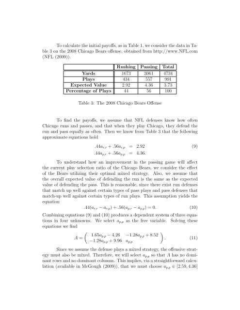
To calculate the initial payoffs, as in Table 1, we consider the data in Table 3 on the 2008 Chicago Bears offense, obtained from http://www.NFL.com (NFL (2009)). Rushing Passing Total Yards 1673 3061 4734 Plays 434 557 991 Expected Value 2.92 4.36 3.73 Percentage of Plays 44 56 100 Table 3: The 2008 Chicago Bears Offense To find the payoffs, we assume that NFL defenses know how often Chicago runs and passes, and that when they play Chicago, they defend the run and pass equally as often. Then we know from Table 3 that the following approximate equations hold .44ar,r + .56ar,p = 2.92 (9) .44ap,r + .56ap,p = 4.36. To understand how an improvement in the passing game will affect the current play selection ratio of the Chicago Bears, we consider the effect of the Bears utilizing their optimal mixed strategy. Also, we assume that the overall expected value of defending the run is the same as the expected value of defending the pass. This is reasonable, since there exist run defenses that match up well against certain types of pass plays and pass defenses that match-up well against certain types of run plays. This assumption yields the equation .44(ar,r − ar,p) + .56(ap,r − ap,p) = 0. (10) Combining equations (9) and (10) produces a dependent system of three equations in four unknowns. We select ap,p as the free variable. Solving these equations we find 1.65ap,p − 4.26 −1.28ap,p + 8.52 A = −1.28ap,p + 9.96 ap,p . (11) Since we assume the defense plays a mixed strategy, the offensive strategy must also be mixed. Therefore, we will select ap,p so that A has no dominant rows and no dominant columns. This implies, via a straightforward calculation (available in McGough (2009)), that we must choose ap,p ∈ [2.59, 4.36]
in order to produce our desired payoff structure: ap,p < ap,r, ar,p > ap,p, ar,r < ar,p, and ar,r < ap,r. For our analysis we choose ap,p = 10, as an offense strives to achieve 3 at least 10 yards on first through third down and the defense wishes to hold 3 them to at most this average. This gives 1.23 4.26 A ≈ 5.70 3.33 and leads to Table 4, the improvement in passing model for the 2009 Bears. Defense Defend Run Defend Pass Offense Run 1.23(1 + δx) 4.26(1 + δx) Pass 5.70(1 + x) 3.33(1 + x) Table 4: The 2009 Chicago Bears Improvement in Passing Model Table 5 gives optimal solutions to the game for selected values of x with δ = 1 2 . Note that when x = 0, R∗ and V represent the proportion of run plays and the average yards per play, respectively, for the Bears in 2008. x 0 0.1 0.2 0.3 0.4 R ∗ 0.439 0.450 0.460 0.469 0.477 ∂R ∗ ∂x 0.123 0.107 0.094 0.083 0.074 P ∗ 0.561 0.550 0.540 0.531 0.523 V 3.738 4.023 4.313 4.596 4.877 Table 5: Optimal Play Balance and Expected Yardage for the 2009 Chicago Bears Observe that in Table 5, the number of running plays called increases as x grows and the passing game improves. This reflects our observations in the previous section. As mentioned above, our calculations will generally use δ = 1 2 . Figure 1 gives the values of R∗ (δ,x) for all δ and x in [0, 1]. The greyscale to the right of the figure gives a measure of R ∗ , with lighter shades reflecting a higher proportion of running plays. For a given δ, the black region in the figure represents those values of x beyond the breaking point.
- Page 1 and 2: 1 Introduction There is a growing i
- Page 3 and 4: on our team’s performance. We ass
- Page 5 and 6: As a notational convenience, let D(
- Page 7: ∂R∗ ∂x = (ar,p − ar,r)(ap,r
- Page 11 and 12: Therefore, if we assume that Jay Cu
- Page 13: Carter, V. and R. Machol (1978):
To calculate the <strong>in</strong>itial payoffs, as <strong>in</strong> Table 1, we consider the data <strong>in</strong> Table<br />
3 on the 2008 Chicago Bears offense, obta<strong>in</strong>ed from http://www.NFL.com<br />
(NFL (2009)).<br />
Rush<strong>in</strong>g Pass<strong>in</strong>g Total<br />
Yards 1673 3061 4734<br />
Plays 434 557 991<br />
Expected Value 2.92 4.36 3.73<br />
Percentage of Plays 44 56 100<br />
Table 3: The 2008 Chicago Bears Offense<br />
To f<strong>in</strong>d the payoffs, we assume that NFL defenses know how often<br />
Chicago runs and passes, and that when they play Chicago, they defend the<br />
run and pass equally as often. Then we know from Table 3 that the follow<strong>in</strong>g<br />
approximate equations hold<br />
.44ar,r + .56ar,p = 2.92 (9)<br />
.44ap,r + .56ap,p = 4.36.<br />
To understand how an improvement <strong>in</strong> the pass<strong>in</strong>g game will affect<br />
the current play selection ratio of the Chicago Bears, we consider the effect<br />
of the Bears utiliz<strong>in</strong>g their optimal mixed strategy. Also, we assume that<br />
the overall expected value of defend<strong>in</strong>g the run is the same as the expected<br />
value of defend<strong>in</strong>g the pass. This is reasonable, s<strong>in</strong>ce there exist run defenses<br />
that match up well aga<strong>in</strong>st certa<strong>in</strong> types of pass plays and pass defenses that<br />
match-up well aga<strong>in</strong>st certa<strong>in</strong> types of run plays. This assumption yields the<br />
equation<br />
.44(ar,r − ar,p) + .56(ap,r − ap,p) = 0. (10)<br />
Comb<strong>in</strong><strong>in</strong>g equations (9) and (10) produces a dependent system of three equations<br />
<strong>in</strong> four unknowns. We select ap,p as the free variable. Solv<strong>in</strong>g these<br />
equations we f<strong>in</strong>d<br />
<br />
1.65ap,p − 4.26 −1.28ap,p + 8.52<br />
A =<br />
−1.28ap,p + 9.96 ap,p<br />
<br />
. (11)<br />
S<strong>in</strong>ce we assume the defense plays a mixed strategy, the offensive strategy<br />
must also be mixed. Therefore, we will select ap,p so that A has no dom<strong>in</strong>ant<br />
rows and no dom<strong>in</strong>ant columns. This implies, via a straightforward calculation<br />
(available <strong>in</strong> McGough (2009)), that we must choose ap,p ∈ [2.59, 4.36]


