A Game-Theoretic Approach to Personnel Decisions in American ...

1 Introduction
There is a growing interest in the application of game theory to American
football. This is natural, since the number of feasible strategies available to a
team are vast, and play selection has a strong impact on the success of a given
play. Coaches who employ the principles of game theory can realize benefits
to their game planning and in-game play calling, resulting in an increase in
their team’s expected efficiency (Jordan, Melouk, and Perry (2009)).
Here, we are interested in determining the optimal proportion of run
and pass plays. Since determining the optimal mix of these plays depends
heavily on a team’s offensive players, a change in personnel can greatly affect
the optimal proportion of pass and run plays. Therefore, a game-theoretic
mindset is crucial when considering trades, signing free agents, and releasing
current players.
This paper utilizes game-theoretic techniques to determine the optimal
proportion of run and pass plays for a team by exploring the relationship
between player personnel and play selection. Specifically, we study how the
acquisition of a proven quarterback affects a team’s run/pass balance. While
we focus on an improvement in a team’s passing game via the quarterback
position, our methods easily extend to any offensive or defensive personnel
change.
There have been several relevant contributions that focus on behavior
exhibited by coaches in critical game situations. Carter and Machol (1978)
analyzed data from the 1971 NFL season that suggests coaches opt for field
goals when the expected point value of “going for it” is much higher. A
similar analysis is captured in the work of Romer (2006), who argues that
coaches should go for it on fourth down in some situations instead of kicking.
Rockerbie (2008) shows that there is a correlation between win percentage and
teams who employ optimal strategies without excessive concern for risk.
All of these analyses have shown that coaches have a tendency to avoid
risk, and do not maximize expected returns. Here, we do not construct a
risk-averse model, instead we choose to disregard the human tendency to be
risk-averse in pressure situations. Our model seeks to determine a team’s
optimal proportion of run and pass plays under the hypothesis that a coach is
risk-indifferent when it comes to calling run plays and pass plays.
We proceed by defining the payoffs and setting up the model. Then
in Section 4, we solve the game and discuss some theoretical results. In Section
5, we apply the results, and examine how the acquisition of Jay Cutler
might impact the run/pass balance of the 2009 Chicago Bears. Afterwards,
we compare our suggested run/pass balance with the one implemented by the

Chicago Bears this past season and some implications due to this comparison.
2 Setting Up the Game
We consider two-by-two zero-sum games where the offense either runs or passes
and the defense either defends against the run or defends against the pass.
Each payoff represents an expected gain for the offense under the given strategic
situation. For any serious football team, it is reasonable to suggest that
the payoffs can be found, since every coaching staff spends much of their time
breaking down film.
Table 1: Initial Payoffs
Defense
Defend Run Defend Pass
Offense Run ar,r ar,p
Pass ap,r ap,p
Let the offensive and defensive strategy sets be {R,P } and {DR,DP },
respectively. Furthermore, let ar,r denote the payoff for (R,DR), ar,p denote
the payoff for (R,DP), and so on, as in Table 1. Throughout this paper, we
make the reasonable assumptions that ar,r < ap,r and ar,p > ap,p.
We calculate the expected gain for the offensive team in a straightforward
manner, save that we adopt a convention used by Alamar (2006) and
Rockerbie (2008) and deduct 45 yards from a team’s total yardage for each
fumble and interception. For instance, to determine ar,r, suppose that there
were nr,r observed plays in which the offense elected to run and the defense
elected to defend the run, amounting in a total of yr,r yards and tr,r turnovers.
Then
ar,r = yr,r − 45tr,r
.
The remaining payoffs in Table 1 are calculated in a similar manner.
nr,r
3 The Improvement in Passing Model
Having demonstrated how to calculate the payoffs for our team prior to the
relevant personnel change, we now model the impact of this personnel change

on our team’s performance. We assume that the team has acquired a proven
quarterback whose presence will improve all aspects of the passing game. This
will be reflected in our payoff table via an increase in both payoff entries
associated with an offensive passing play.
The following additional assumption is a critical part of our model. It
is a common belief that the success of the passing game is intertwined with the
success of the running game. Consequently, we suppose that the increase in
expected gains through passing will also have a positive effect on the running
payoffs ar,r and ar,p. Although the quarterback will positively influence the
running game, he will have a greater impact on the passing game. This is
because production in the passing game rests squarely upon his ability and
performance, whereas the quarterback’s influence is generally limited in the
running game. We now introduce the model.
Throughout this analysis, we assume that the payoff matrix depicted
in Table 1 contains no dominant rows and no dominant columns, implying
that our games will have only mixed strategy Nash equilibria (Nash (1951)).
This assumption is reasonable in the context of our desired applications, as
it is unlikely that a serious amateur or professional football team would ever
utilize a pure offensive strategy.
We let x represent the proportional increase in the passing game for
some real x > 0 and let δ measure the residual effect of the improved passing
game on the running game. We conceptualize x as a (relative) quarterback
rating, so that if x = 0, the new quarterback is no better than the previous one.
These parameters are incorporated into the payoffs from Table 1 to obtain the
2-by-2 game in 2, which reflects the assumed changes in player personnel. We
refer to this as the improvement in passing model .
Defense
Defend Run Defend Pass
Offense Run ar,r(1 + δx) ar,p(1 + δx)
Pass ap,r(1 + x) ap,p(1 + x)
Table 2: The Improvement in Passing Model
Comparing mobile quarterbacks and pocket passers of the same caliber,
it is reasonable to suggest that mobile quarterbacks have a higher δ value,
since they are contributing to both phases of the game. In the case of a highly
immobile quarterback with a strong arm, the value of δ for each quarterback
could, in fact, be negative, even if x is relatively high. While this is feasible,

and the model is readily adaptable to accommodate this possibility, we will
assume for simplicity that δ ∈ [0, 1].
In our simulations, we generally suppose that δ = 1,
although we un-
2
dertake an examination of our results for a number of values of δ in Section
6. It is important to mention that each quarterback corresponds to exactly
one x rating. While this rating may increase or decrease over the course of a
player’s career, at any given moment it is fixed.
4 Solving the Model
We solve the improvement in passing model analytically and determine Nash
equilibria for the proportion of run (and pass) plays depending on x,δ and the
values in Table 1.
First, assume that both the offense and defense are playing optimally.
Let pr be the probability that the offense calls a running play. The Nash equilibrium
value for the proportion of running plays will arise when the defensive
team is strategy-indifferent. That is, a Nash equilibrium occurs when the
expected value of the “Defend Run” and “Defend Pass” strategies are equal
under the assumption that on each play the offensive coach elects to run the
ball independently with probability pr. Then R(δ,x), the Nash equilibrium
value for the proportion of running plays, is the value of pr that solves the
following equation:
ar,r(1 + δx)pr + ap,r(1 + x)(1 − pr) = ar,p(1 + δx)pr + (1 + x)ap,p(1 − pr). (1)
After some elementary algebra, we obtain
R(δ,x) =
(ap,r − ap,p)(1 + x)
. (2)
(ar,p − ar,r)(1 + δx) + (ap,r − ap,p)(1 + x)
Observe that R(δ,x) depends on the quantities (ar,p − ar,r) and (ap,r −
ap,p). These terms measure the benefit of a running or passing play, respectively,
carried out against the “wrong” defense. For instance, if (ar,p − ar,r)
is large relative to (ap,r − ap,p), then there is more added benefit for a team
to run against a pass defense than it is to pass against a run defense (relative
to each play being carried out against an appropriate defense). Interestingly,
and somewhat counterintuitively, this bonus for a team to “guess right” with
a running play results in a smaller overall proportion of running plays being
called.

As a notational convenience, let
D(δ,x) = (ar,p − ar,r)(1 + δx) + (ap,r − ap,p)(1 + x).
To find the defensive Nash equilibrium functions, we perform a similar calculation
to that used to obtain (2). The defensive Nash equilibrium functions
are
Rdef(δ,x) = (ar,p
and
− ap,p) + x(δar,p − ap,p)
D
(3)
Pdef(δ,x) = 1 − Rdef(δ,x) (4)
where Rdef(δ,x) and Pdef(δ,x) denote the Nash equilibrium proportions for
run defense and pass defense, respectively.
These equilibria provide optimal mixed strategy solutions to the game
in terms of x and δ. We limit x to the closed interval [0, 1], because large values
of x result in unreasonable increases in the expected yards per play, even for
reasonable choices of ar,r, ar,p, ap,r, and ap,p. We feel that the assumption
that a new quarterback will at most double the passing efficiency of a team is
reasonable, and again the model is readily adaptable.
Next, note that since (1+x) > (1+δx), there may exist some x0 ∈ (0, 1]
such that the passing row in Table 2 will be dominant for all x ≥ x0. We refer
to this value as the breaking point of the model, since it is the point where the
offense would logically transition to a pure strategy. We note that breaking
points do not always exist in (0, 1], and in these cases, the game is a mixed
strategy game for all x ∈ (0, 1]. In fact, we put forth that the presence of
a breaking point in our model provides a reasonable bound on the value of
x, as it does not seem realistic that new player personnel would lead a team
to completely abandon the running game, even if this may be called for in a
narrow set of game situations.
However, in the case that a breaking point does exist in (0, 1], the
following development is necessary for completeness. Recall that we assume
ar,r < ap,r and ar,p > ap,p. Under these assumptions, the breaking point
is easily computed as the value of x satisfying the equation ap,p(1 + x) =
ar,p(1 + δx). The following proposition reflects this.
Proposition 1 If ar,r < ap,r and ar,p > ap,p, then the breaking point of the
game given in Table 2 is
(ar,p − ap,p)
(ap,p − δar,p) .

Thus, the breaking point is a function of δ and the initial payoffs. As one
would expect, the offense and defense converge to a pure strategy at the breaking
point, as evidenced by the fact that Pdef(δ, (ar,p−ap,p) (ar,p−ap,p)
) = P(δ, ) =
(ap,p−δar,p) (ap,p−δar,p)
1. To account for the defensive change from a mixed strategy to a pure strategy
at the breaking point, we give the following discontinuous Nash equilibrium
running function when x ≥ 0.
R ∗ ⎧ (ap,r−ap,p)(1+x)
⎨ D
(δ,x) =
⎩
0 otherwise.
0 ≤ x < (ar,p−ap,p)
(ap,p−ar,pδ) ,
Similarly, we define the discontinuous Nash equilibrium passing function
to be P ∗ (δ,x) = 1 − R ∗ (δ,x). The running function R ∗ encompasses the
above discussion that there is a mixed strategy solution prior to the breaking
point, and that after the breaking point has been reached, quarterback play
has become so influential that the offense only passes.
Next, we calculate V , the value of the game expressed in Table 2. If x
is past the breaking point, then V = ap,p(1 + x), as both teams pursue a pure
strategy. Otherwise, we simply evaluate either side of Equation (1) at R(δ,x).
After simplifying, we obtain the following expression for the value of the game
V (δ,x) = (1 + δx)(1 + x)(ar,pap,r − ap,par,r)
. (6)
D
Observe that (ar,pap,r − ap,par,r) = 0 since the payoff matrix A has no
dominant rows or columns, and hence its rows and columns are necessarily
linearly independent. Since V depends on the nature of the game, it is likely a
discontinuous function of x at the breaking point. Under our assumption that
ap,r > ap,p we obtain the following expression for the value of the game when
x ≥ 0.
V ∗ ⎧ (1+δx)(1+x)(ar,pap,r−ap,par,r)
⎨
D
(δ,x) =
⎩
ap,p(1 + x) otherwise.
0 ≤ x < (ar,p−ap,p)
(ap,p−δar,p) ,
Before we proceed with our predictive example, we examine an interesting
and unexpected property of R ∗ . For values of x less than the breaking
point, we observe that
(5)
(7)

∂R∗ ∂x = (ar,p − ar,r)(ap,r − ap,p)(1 − δ)
D2 . (8)
Our assumption about the initial payoffs, specifically that ar,p > ar,r
and ap,r > ap,p imply that ∂R∗ > 0. This is quite unexpected, as it suggests
∂x
that as a team’s passing game improves, the team should actually pass less
than it did previously!
5 Predicting the Impact of Jay Cutler on the
Play Selection of the 2009 Chicago Bears
In this section, we utilize our model to make a prediction relevant to the 2009
NFL season by considering the effect of new quarterback Jay Cutler on the
play selection of the Chicago Bears. Recall that to find the payoffs for Table
1 in the manner described above, the defensive strategies “Defend Run” and
“Defend Pass” must be clearly defined and the number of times each strategy
is employed must be accurately tallied. In our computational analysis below,
we utilize data from past NFL seasons, but we do not explicitly determine
the number of times the defense chose each strategy. Instead, we attempt to
approximate these values. While this is not optimal, we again point out that
a serious team’s coaching staff would have ready access to the necessary data.
In his fourth NFL season, Jay Cutler is among the more promising
young quarterbacks in the league. In the 2008 season, he finished 3 rd in the
NFL in total passing yardage and was subsequently traded from Denver to
Chicago. For Bears fans, this is good news, since in the past five seasons the
Chicago Bears have finished no better than 14 th in the NFL in total passing
yardage. With an improvement in passing, Chicago figured to be competitive
in the NFC. The following analysis aims to examine how the acquisition of
Jay Cutler might alter the run/pass balance of the Chicago Bears for the 2009
season.
We first construct the payoff matrix for the Chicago Bears using empirical
data from the 2008 season. This data determines the values of the initial
payoffs for the improvement in passing model, as outlined in Section 3. Then,
to predict how the mixed strategies change for Chicago, we explore how Jay
Cutler influenced the expected yardage per play in his first season as a starter
in Denver. Once this influence is known, we project it onto the 2009 Chicago
Bears improvement in passing model.

To calculate the initial payoffs, as in Table 1, we consider the data in Table
3 on the 2008 Chicago Bears offense, obtained from http://www.NFL.com
(NFL (2009)).
Rushing Passing Total
Yards 1673 3061 4734
Plays 434 557 991
Expected Value 2.92 4.36 3.73
Percentage of Plays 44 56 100
Table 3: The 2008 Chicago Bears Offense
To find the payoffs, we assume that NFL defenses know how often
Chicago runs and passes, and that when they play Chicago, they defend the
run and pass equally as often. Then we know from Table 3 that the following
approximate equations hold
.44ar,r + .56ar,p = 2.92 (9)
.44ap,r + .56ap,p = 4.36.
To understand how an improvement in the passing game will affect
the current play selection ratio of the Chicago Bears, we consider the effect
of the Bears utilizing their optimal mixed strategy. Also, we assume that
the overall expected value of defending the run is the same as the expected
value of defending the pass. This is reasonable, since there exist run defenses
that match up well against certain types of pass plays and pass defenses that
match-up well against certain types of run plays. This assumption yields the
equation
.44(ar,r − ar,p) + .56(ap,r − ap,p) = 0. (10)
Combining equations (9) and (10) produces a dependent system of three equations
in four unknowns. We select ap,p as the free variable. Solving these
equations we find
1.65ap,p − 4.26 −1.28ap,p + 8.52
A =
−1.28ap,p + 9.96 ap,p
. (11)
Since we assume the defense plays a mixed strategy, the offensive strategy
must also be mixed. Therefore, we will select ap,p so that A has no dominant
rows and no dominant columns. This implies, via a straightforward calculation
(available in McGough (2009)), that we must choose ap,p ∈ [2.59, 4.36]

in order to produce our desired payoff structure: ap,p < ap,r, ar,p > ap,p,
ar,r < ar,p, and ar,r < ap,r.
For our analysis we choose ap,p = 10,
as an offense strives to achieve
3
at least 10 yards on first through third down and the defense wishes to hold
3
them to at most this average. This gives
1.23 4.26
A ≈
5.70 3.33
and leads to Table 4, the improvement in passing model for the 2009 Bears.
Defense
Defend Run Defend Pass
Offense Run 1.23(1 + δx) 4.26(1 + δx)
Pass 5.70(1 + x) 3.33(1 + x)
Table 4: The 2009 Chicago Bears Improvement in Passing Model
Table 5 gives optimal solutions to the game for selected values of x with
δ = 1
2 . Note that when x = 0, R∗ and V represent the proportion of run plays
and the average yards per play, respectively, for the Bears in 2008.
x 0 0.1 0.2 0.3 0.4
R ∗ 0.439 0.450 0.460 0.469 0.477
∂R ∗
∂x 0.123 0.107 0.094 0.083 0.074
P ∗ 0.561 0.550 0.540 0.531 0.523
V 3.738 4.023 4.313 4.596 4.877
Table 5: Optimal Play Balance and Expected Yardage for the 2009 Chicago
Bears
Observe that in Table 5, the number of running plays called increases
as x grows and the passing game improves. This reflects our observations in
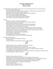
the previous section. As mentioned above, our calculations will generally use
δ = 1
2 . Figure 1 gives the values of R∗ (δ,x) for all δ and x in [0, 1]. The
greyscale to the right of the figure gives a measure of R ∗ , with lighter shades
reflecting a higher proportion of running plays. For a given δ, the black region
in the figure represents those values of x beyond the breaking point.

δ
1
0.9
0.8
0.7
0.6
0.5
0.4
0.3
0.2
0.1
R* Coloring the Unit Square
0
0 0.2 0.4 0.6 0.8 1
x
Figure 1: R ∗ (δ,x) using 2008 Chicago Bears Data
As can be seen in Figure 1, the breaking point when δ = 1 (as in 2
our calculations) is approximately 0.775. This implies that to be justified
in playing a pure pass strategy, the expected yards per play would have to
increase by approximately 2.178 yards. This is a large increase, and supports
our claim that it is unrealistic to anticipate that Chicago would ever pursue a
pure passing strategy.
In order to examine how Jay Cutler impacts the run/pass balance of
the Chicago Bears, we first find his x. To do so, we will consider Cutler’s
effect on the Broncos’ offense in 2007, his first year as a starter. We begin
using the data from the 2006 Broncos offense to calculate Table 6, Denver’s
2007 improvement in passing model, in a manner similar to our development
of Table 4.
Defense
Defend Run Defend Pass
Offense Run 2.73(1 + δx) 4.25(1 + δx)
Pass 4.86(1 + x) 3.33(1 + x)
Table 6: The 2007 Denver Broncos Improvement in Passing Model
In 2007, the Broncos gained an average of 4.57 yards per play. Thus,
the x-value that we seek for Jay Cutler is the solution to V ∗ ( 1,x)
= 4.57,
2
where V ∗ is as given in (7). Solving, we obtain x ≈ 0.279.
1
0.9
0.8
0.7
0.6
0.5
0.4
0.3
0.2
0.1
0

Therefore, if we assume that Jay Cutler has a similar influence in
Chicago to the one he had in Denver, then substituting x ≈ 0.279 into Table
4, the Chicago Bears improvement in passing model, and performing the necessary
calculations, gives that the Bears should expect an overall increase of
about 0.799 yards per play.
Also, quite interestingly, because of this anticipated improvement in
passing, our model indicates that the Bears should call about 3% more running
plays this season and implement a 47 : 53 run/pass ratio. While these
results are not overwhelmingly significant, from a coaching standpoint they are
valuable. They suggest that a strong emphasis should be placed on developing
the running game in training camp and during the pre-season, since it should
be a central focus on Sunday afternoons.
2009 was a season to forget for the Chicago Bears. After beginning the
season 3-1, the Bears finished the season an abysmal 7-9. The Bears struggled
all season running the football and were held to an NFC worst 93.2 yards per
game. Meanwhile, some would argue, they remained overly committed to the
passing game, calling a pass play 62% of the time. This idea was echoed by
Bears six-time Pro Bowl linebacker Brian Urlacher who said,“Look, I love Jay,
and I understand he’s a great player who can take us a long way, and I still
have faith in him. But I hate the way our identity has changed. We used to
establish the run and wear teams down and try not to make mistakes, and
we’d rely on our defense to keep us in the game and make big plays to put us
in position to win. Kyle Orton might not be the flashiest quarterback, but the
guy is a winner, and that formula worked for us. I hate to say it, but that’s
the truth (Urlacher (2010)).” In 2008, the Bears’ run/pass ratio was 44 : 56,
gaining approximately 3.74 yards per play. In 2009, with the acquisition of
Jay Cutler, the Bears’ run/pass ratio was 38 : 62, gaining approximately 3.68
yards per play. Our model suggests that the Bears should have called a run
play about 47% of the time. For our model, their allocation of run and pass
deviates 9% from our result, implying that the Bears were playing far from
optimally. Although these results do not validate our prediction, they do give
some explanation as to why the Bears underachieved in 2009.
6 Summary and Extensions
This paper discusses how player personnel changes alter the run/pass balance
of an offense. Our conclusions have far-reaching implications. Quite unexpectedly,
our results suggest that if a team acquires new personnel that will

improve their expected returns in passing, without a corresponding change to
their running personnel, they should pass less than they did a season ago.
This analysis also extends to different phases of the game, offensively
and defensively. If a team trades for a lock-down cornerback, the defensive coordinator
should blitz more. If the offense signs a talented running back, they
should pass more. This analysis describes the value of players, since if a team
signs John Doe, then they are able to say “he allots us freedom in this way.”
Of course, this can become complicated when a team drafts several players.
However, it is reasonable to suppose that there is a positive correlation between
the order in which the players are drafted and the immediate utility they
contribute to the organization. Thus, given a draft ordering of players, and
their comparative strengths and weaknesses, it is possible to understand how
the play selection changes on offense and defense using these game-theoretic
arguments.
We note the limitations of the model. First of all, the choice of δ is ad
hoc, however its presence is unavoidable. The accuracy of the model could be
improved by developing a more sophisticated relationship between the value
of x and the resultant increase in the running game. Secondly, the projection
of x, found by examining past Denver Bronco’s data, onto the 2008 Chicago
Bears improvement in passing model is debatable. Clearly, the increase in
expected yardage per play for Denver from the 2006 season to the 2007 season
was not due solely to Jay Cutler’s production. With that said, it is always true
that a quarterback rating reflects both the statistical makeup of a quarterback
and the quality of his supporting cast. Ideally, the choice of x would reflect
a more complete analysis of the passing game from year to year, involving
statistical methods to analyze a larger collection of players.
Finally, our ultimate vision for this model supports the construction
of a more complete payoff matrix, consisting of a larger number of offensive
and defensive strategies. Ideally, trends, strengths, and weaknesses would be
considered to enable an approach that is more adaptable week-by-week. As
difficult as this sounds, it can be done by breaking down film of NFL games.
All of these extensions would aid in the development of coaching strategy,
which in turn, would cause the game to evolve.
References
Alamar, B. (2006): “The passing premium puzzle,” Journal of Quantitative
Analysis in Sports, 2(4), Article 5.

Carter, V. and R. Machol (1978): “Optimal strategies on fourth down,” Management
Science, 24(16), 1758–1762.
Jordan, J., S. Melouk, and M. Perry (2009): “Optimizing football game play
calling,” Journal of Quantitative Analysis in Sports, 5(2), Article 2.
McGough, E. (2009): Analyzing the Relationship Between Player Personnel
and Optimal Mixed Strategies in American Football, Master’s thesis, The
University of Akron.
Nash, J. (1951): “Non-cooperative games,” Ann. Math., 54, 286–295.
NFL (2009): “Nfl statistics,” World Wide Web electronic publication, URL
http://www.nfl.com.
Rockerbie, D. (2008): “The passing premium puzzle revisited,” Journal of
Quantitative Analysis in Sports, 4(2), Article 5.
Romer, D. (2006): “Do firms maximize? evidence from professional football,”
Journal of Political Economy, 114(2), 340–365.
Urlacher, B. (2010): “Struggles with sideline role,” World Wide Web electronic
publication, URL http://sports.yahoo.com/nfl/.