Introduction to Calculus-Lab 1 1) Solve the following inequalities 1.1 ...

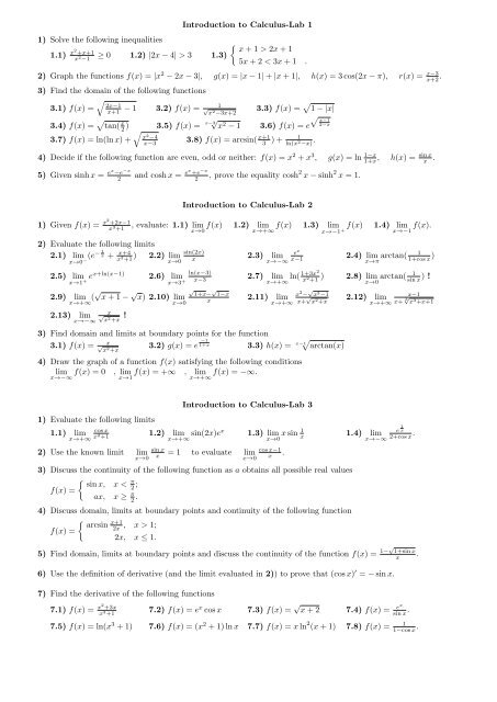
1) Solve the following inequalities
1.1) x2 +x+1
x 2 −1
≥ 0 1.2) |2x − 4| > 3 1.3)
Introduction to Calculus-Lab 1
x + 1 > 2x + 1
5x + 2 < 3x + 1 .
2) Graph the functions f(x) = |x 2 − 2x − 3|, g(x) = |x − 1| + |x + 1|, h(x) = 3 cos(2x − π), r(x) = x−3
x+2 .
3) Find the domain of the following functions
2x−1
3.1) f(x) = x+1 − 1 3.2) f(x) = √ 1 3.3) f(x) =
x2−3x+2 1 − |x|
3.4) f(x) = tan( x
2 ) 3.5) f(x) = x−3√ x2
x−1
2−x
− 1 3.6) f(x) = e
x2−4 3.7) f(x) = ln(ln x) + x−3 3.8) f(x) = arcsin( x+1
3 ) + 1
ln(x2−x) .
4) Decide if the following function are even, odd or neither: f(x) = x2 + x3 , g(x) = ln 1−x
sin x
1+x , h(x) = x .
5) Given sinh x = ex −e −x
2
and cosh x = ex +e −x
2 , prove the equality cosh 2 x − sinh 2 x = 1.
Introduction to Calculus-Lab 2
1) Given f(x) = x2 +2x−1
x3 +1 , evaluate: 1.1) lim f(x) 1.2) lim f(x) 1.3) lim
x→0 x→+∞ x→−1 +
f(x) 1.4) lim
x→−1 f(x).
2) Evaluate the following limits
2.1) lim
x→0− 1 − (e x + x+4
x2 +1 ) 2.2) lim
x→0
2.5) lim
x→1 +
ex+ln(x−1) 2.6) lim
x→3 +
2.9) lim
x→+∞ (√ x + 1 − √ x) 2.10) lim
x→0
2.13) lim
x→−∞
x
√ x 2 +x !
sin(2x)
x 2.3) lim
x→−∞
ln(x−3)
x−3 2.7) lim
x→+∞
e x
x−1
√ √
1+x− 1−x
x
x 2.11) lim
x→+∞
2 − √ x3−1 x+ √ x2 +x
3) Find domain and limits at boundary points for the function
3.1) f(x) = x
√ x 2 +x
3.2) g(x) = e −1
1+x 3.3) h(x) = x−1 arctan(x)
4) Draw the graph of a function f(x) satisfying the following conditions
lim f(x) = 0
x→−∞
, lim f(x) = +∞
x→1
, lim f(x) = −∞.
x→+∞
1) Evaluate the following limits
1.1) lim
x→+∞
Introduction to Calculus-Lab 3
2.4) lim
x→π arctan( 1
1+cos x )
1+3x2 ln( x2 1
+1 ) 2.8) lim arctan(
x→0 sin x ) !
2.12) lim
x→+∞
cos x
x 2 +1 1.2) lim
x→+∞ sin(2x)ex 1.3) lim
x→0 x sin 1
x 1.4) lim
x→−∞
sin x
2) Use the known limit lim
x→0 x
= 1 to evaluate lim
x→0
cos x−1
x .
3) Discuss the continuity of the following function as a obtains all possible real values
π
sin x, x < 2
f(x) =
;
ax, x ≥ π
2 .
4) Discuss domain, limits at boundary points and continuity of the following function
x+1 arcsin 2x , x > 1;
f(x) =
2x, x ≤ 1.
x−1
x+ 3√ x 3 +x+1
e 1 x
2+cos x .
5) Find domain, limits at boundary points and discuss the continuity of the function f(x) = 1−√1+sin x
x .
6) Use the definition of derivative (and the limit evaluated in 2)) to prove that (cos x) ′ = − sin x.
7) Find the derivative of the following functions
7.1) f(x) = x2 +3x
x 3 +1 7.2) f(x) = e x cos x 7.3) f(x) = √ x + 2 7.4) f(x) = ex
sin x .
7.5) f(x) = ln(x 3 + 1) 7.6) f(x) = (x 2 + 1) ln x 7.7) f(x) = x ln 2 (x + 1) 7.8) f(x) = 1
1−cos x .

Introduction to Calculus-Lab 4
1) Use the bisection method to find a solution of the equation x 3 − 2x 2 + x − 4 = 0 with an approximation of
two decimal points.
2) Use the bisection method to find the intersection point of the graphs of y = e x and y = −x with an
approximation of two decimal points.
2) Find the tangent line and orthogonal line to the graph of the function f(x) = ln(x 2 +3x+1)+e x2 +1 at x = 0.
3) Find the equation of the line passing trough the origin and tangent to the graph of f(x) = ln x.
4) Find the derivative of the following function and compare its domain with the domain of the original function:
4.1) f(x) = ln( x2 +3x
x 3 +1 ) 4.2) f(x) = ex cos x
ln 2 x
4.3) f(x) =
√ ln(x+2)
x 2 4.4) f(x) = √ e x +1
x 2 +sin 2 x
4.5) f(x) = ln e x (x 3 ) 4.6) f(x) = √ x ln 2 x 4.7) f(x) = x 2(x+1) 4.8) f(x) = (x + 1) cos2 x .
5) Use l’Hospital’s rule the calculate the following limits:
5.1) lim x ln(x) 5.2) lim
x→0 + x→0 +
e 5.5) lim
x→0
x −1
x 5.6) lim
x→+∞
e x −1
cos x−1
√ x+1
ln 2 (x+1)
5.3) lim
x→0 + xx 5.4) lim
x→+∞
5.7) lim (1 + x)
x→0 1
x 5.8) lim
x→0 +
( 1
x
x 2 +3x
ln(x 3 +1)
− 1
sin x ).
6) Determine for what values of a, b ∈ IR the following function is continuous and differentiable in all its domain
π
sin x, x < 2
f(x) =
;
ax + b, x ≥ π
2 .
1) Find the derivative of the following function
Introduction to Calculus-Lab 5
1.1) f(x) = ln(1 + |x − 1|) 1.2) f(x) = arctan 1+x
1−x .
2) Find the Taylor polynomial of degree n at a = 0 for the function
2.1) f(x) = 1
1+x
2.2) f(x) = e 2x .
3) Find the Taylor polynomial of third degree at a = 1 for the function f(x) = x ln x.
4) Find maximal intervals where the function is increasing, decreasing, local maximum and minimum for
f(x) = e x2 +3x−|x| .
5) Find absolute maximum and minimum of f(x) = x 2 − 8|x − 1| + 8 in the closed interval [−1, 6].
6) After determining maximal intervals where the function is increasing (decreasing), local maximum, minimum,
maximal intervals where the function is concave up (down) and inflexion points, graph the function
6.1) f(x) = x + |x| 6.2) f(x) = |x|e x 6.3) f(x) = x3
x 2 −1
Introduction to Calculus-Lab 6
6.4) f(x) = 3x 4 − 8x 3 + 6x 2 .
1) Find maximal intervals where the following function is concave up and concave down, inflexion points.
1.1) f(x) = x ln 2 x 1.2) f(x) = x3 − |x| 3 + 3x2. − 12x
2) Write down the equation of all asymptotes of the following functions
2.1) f(x) = x2 +x−1
x−1 2.2) f(x) = xex
e x −e −x
2.3) f(x) = √ x
ln x
2.4) f(x) = x ln(1 + 1
x ).
3) Find domain, limits at boundary point, asymptotes, maximal intervals where the function is increasing (decreasing),
local maximum, minimum, maximal intervals where the function is concave up (down), inflexion
points, and graph the function
3.1) f(x) = 1 + ln |x| 3.2) f(x) = xe−x 3.3) f(x) = ln( |x−1|
|x−1|
x+1 ) 3.4) f(x) = arctan( x ).

Introduction to Calculus-Lab 7
- Evaluate the following integrals
1) 2x cos(x 2
) dx 2) cos x sin 2
x dx 3)
4)
2
dx
3 − x
5)
2√ 1
ex −
1 − √ 7)
xe
dx
x
6)
2x dx 8)
x 2 sin( x
10)
13)
ln x
dx
x
sin
11)
) dx
2
arctan x dx
9)
12)
√ x dx 14)
ln 2 x dx 15)
16)
e2x e2x dx 17)
+ 1
- Evaluate the following integrals
1) (2x − 1) sin(x − 2) dx 2)
4)
√x √
sin x dx 5)
7)
10)
13)
1
x2 dx 8)
− 1
6
e2x − ex dx 11)
− 2
1
ex dx 14)
− 4e−x A) Evaluate the following integrals
1)
4)
7)
10)
π
0
1
0
2
0
π
0
(2x + 1) cos(x + π) dx 2)
e x+2 cos(e x + π) dx 5)
4x + 5
x2 dx 8)
+ 1
sin 3 (x) dx 11)
1
x(1 + ln 2 dx 18)
x)
Introduction to Calculus-Lab 8
(3x + 1) cos( x
) dx 3)
π
x 3 x 2 + 1 dx 6)
1
x3 dx 9)
− 1
5x2 + 6x + 2
x2 (x2 dx 12)
+ 2x + 2)
x2 + x
(x − 1)(x2 dx 15)
+ 1)
Introduction to Calculus-Lab 9
3
2
π
0
1
0
x
dx 3)
(x − 1) 3
2 sin 2 ( x
) dx 6)
2
2x 3 − 3x 2 + 1
x 2 + 16
B) The following calculation is wrong. Explain why.
2
1
= −
x2 1
2 x
= − 1
− 1 = −3
2 2 .
−1
−1
5
2
dx 9)
5
√ x − 1 + 2 dx 12)
e 2x−3 dx
1
√ 1 − x 2 dx
3x ln(2x) dx
x 3 sin(x 2 ) dx
arcsin x dx
x sin x
cos 3 x dx
x 2 + 2e x (x + e x ) dx
4x
√ 2x − 1 dx
2 2x + 3x + 18
x3 dx
+ 9x
(4 sin x + 6) cos x
(sin(x) − 1)(sin 2 (x) + 4) dx
5(sin(x) + 2) cos x
(sin(x) + 1)(5 − cos2 (x)) dx
4
1
1
0
3
1
2
0
x + 5
√ x + 1 dx
(2x − 5) ln(x + 1) dx
2x 2 + 2
x 3 + 2x 2 + 2x dx
(x − |x − 1|)e x dx
C) Use a partition of the interval [π, 2π] and the definition of definite integral to approximate the value of
2π
sin x
x dx.
π

- Evaluate the following improper integrals
1)
4)
7)
10)
13)
16)
∞
0
1
0
∞
0
∞
0
−1
−∞
4
0
−1
dx 2)
(x + 2)(x + 1)
1
x2 dx 5)
− 2x
1 1
e− x dx 8)
x2 ex e2x dx 11)
+ 1
1
x √ dx 14)
1 − x
1
√ x(1 + x) dx 17)
Introduction to Calculus-Lab 10
∞
−∞
∞
3
∞
0
∞
0
1
−1
+∞
1) Use the definition to find the Laplace transform of
0
1
dx 3)
1 + x2 1
x2 dx 6)
− 2x
1
x2 dx 9)
− 2x + 5
1
ex dx 12)
+ 1
1
x2 dx 15)
− 2|x| + 1
xe −2x dx 18)
Introduction to Calculus-Lab 11
f(t) =
⎧
⎪⎨
⎪⎩
0 t < 0
t 0 ≤ t ≤ 4
4 4 < t ≤ 6
−2t + 16 6 < t ≤ 8
0 t > 8
2) Use the definition to prove that L{cos t} = p
p2 +1 , for p > 0.
3) Find the Laplace transform of the following functions
3.1) f(t) = 3t 2 + 2 cos t 3.2) f(t) = e 2t + 2te −t
3.3) f(t) = 3t sin t + 4 cos t 3.4) f(t) = t 3 e t
3.5) f(t) = (t 2 + 1) sin(2t) 3.6) f(t) = 1 + t sin(t)e t
3.7) f(t) =
sin t
t
+∞
1
∞
0
∞
3
π
2
0
0
−∞
+∞
3.8) f(t) = t(1 + 3t)e 2t
0
e −2x−3 dx
1
x 2 − 2x dx
1
x 2 − x − 2 dx
1
sin x dx
e x
e x + 3 dx
(sin x)e −x dx

Introduction to Calculus-Lab 12
1) Find an inverse Laplace transform of the following functions
1.1) F (p) =
1.3) F (p) =
15
p 2 + 4p + 13
p − 2
p 2 − 2p + 5
1.5) F (p) = 1
p 3 + p
1.7) F (p) = −4p
(p 2 + 4) 2
1.2) F (p) =
1.4) F (p) =
1.6) F (p) =
1.8) F (p) =
p + 1
p 2 + 6p + 25
5p
(p − 1)(p 2 + 4)
p + 1
(p − 2) 3
1
(p − 4) 3
2) Using the Laplace transform, find the solution of the following equation satisfying the given initial conditions:
2.1) y ′′ − y ′ − 2y = 3e −2t , y(0 + ) = 3, y ′ (0 + ) = 3.
2.2) y ′′ − 3y ′ + 2y = e 3t , y(0 + ) = 1, y ′ (0 + ) = 0.
2.3) y ′′ − y ′ = 4te −t , y(0 + ) = 0, y ′ (0 + ) = −1.
2.4) y ′ + 4y + 13 t
0 y(u) du = 1, y(0+ ) = 1.
3) Using the Laplace transform solve the following system.
x ′ = 2x − 4y + 4e −2t x(0 + ) = 2
y ′ = 2x − 2y y(0 + ) = 2
Introduction to Calculus-Lab 13
1) Without using the definition, find the Laplace transform of
f(t) =
⎧
⎪⎨
⎪⎩
0 t < 0
t 0 ≤ t ≤ 4
4 4 < t ≤ 6
−2t + 16 6 < t ≤ 8
0 t > 8
2) Find an inverse Laplace transform of the following functions
1.1) F (p) =
g(t) =
p + e−p
p 2 1.2) F (p) = 2e−p
(p + 5) 3
⎧
⎪⎨
⎪⎩
0 t < 1
2 1 ≤ t < 2
t 2 ≤ t < 6
t 2 − 12 4 ≤ t < 6
0 t ≥ 6
3) Using the Laplace transform, find the solution of the following equation satisfying the given initial conditions:
3.1) y ′′
1,
+ y =
0,
t ∈ [0, π/2)
t ∈ [π/2, ∞),
y(0+) = 1, y ′ (0+) = 0.
3.2) y ′
5 cos(2t), 0 ≤ t < π/2
+ y =
0, t ≥ π/2,
3.3) y ′′
π − t, t ∈ [0, π)
+ y =
0 , t ∈ [π, ∞),
3.4) y ′′ + 2y ′
−2, 0 ≤ t < 1
+ 2y =
t2 − 2, t ≥ 1,
y(0+) = 1.
y(0+) = π, y ′ (0+) = 0.
y(0+) = −1, y ′ (0+) = 0.

Introduction to Calculus-Lab 14
1) Evaluate the convolution f ∗ g of the following functions ⎧
⎪⎨ 0 t < 0
1.1) f(t) = t, g(t) = sin t 1.2) f(t) = g(t) = 1
⎪⎩
0
0 ≤ t < 1
t ≥ 1
2) Using the Laplace transform, find the solution of the following integro-differential equations:
2.1) x ′ + t
0 cosh(t − u)x(u) du = e−t , x(0 + ) = 0.
2.2) y(t) = 4t − 3 t
0
y(u) sin(t − u) du.
2.3) y ′ (t) = sin t + t
0 y(t − u) cos u du, y(0+ ) = 0.
2.4) y ′ + 4y + 4 t
0 y(u) du = 9et − 1, y(0 + ) = 2.
2.5) y ′ (t) + 2y + t
0 y(u) du = sin t, y(0+ ) = 1.
3) Using the Laplace transform solve the following systems.
′ x
3.1)
= t −x + y + e x(0 + y
) = 0
′ = x − y + et y(0 + ) = 0
3.2)
x ′ = x + y x(0 + ) = 2
y ′ = 4x + y y(0 + ) = 3
Introduction to Calculus-Lab 15
1) Find the area of the region bounded by the curves y = √ x, y = √ 2 − x, y = 0.
2) Find the volume of the solid of rotation obtained rotating the region under the graph of y = arcsin x, with
x ∈ [0, 1], around the x-axis.
3) Use an integral to find the area of the surface of the cone with base radius r and hight h.
4) Using 40 metres of fence we need to surround three sides of a rectangular region of the garden with the fourth
side formed by the house wall. What are the measures of the rectangle’s sides that make the area of the
surrounded garden maximal?
5) An isosceles trapezoid has three consecutive sides equal to 10 cm, find the size of the fourth side that makes
maximal the area of the trapezoid.
6) Consider the finite region R bounded by the curves y = sin(x 2 ), y = 1, x = 0. Find the volume of the solid
obtained by revolving the region R about the y-axis.