CARTOGRAPHIC GENERALIZATION IN A DIGITAL ENVIRONMENT ...
CARTOGRAPHIC GENERALIZATION IN A DIGITAL ENVIRONMENT ...
CARTOGRAPHIC GENERALIZATION IN A DIGITAL ENVIRONMENT ...

Create successful ePaper yourself
Turn your PDF publications into a flip-book with our unique Google optimized e-Paper software.
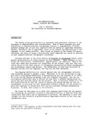
<strong>CARTOGRAPHIC</strong> <strong>GENERALIZATION</strong> <strong>IN</strong> A <strong>DIGITAL</strong> <strong>ENVIRONMENT</strong>:<br />
WHEN AND How To GENERALIZE<br />
K. Stuart Shea<br />
The Analytic Sciences Corporation (TASC)<br />
12100 Sunset Hills Road<br />
Reston, Virginia 22090<br />
Robert B. McMaster<br />
Department of Geography<br />
Syracuse University<br />
Syracuse, New York 13244-1160<br />
ABSTRACT<br />
A key aspect of the mapping process cartographic generalization plays a<br />
vital role in assessing the overall utility of both computer-assisted map<br />
production systems and geographic information systems. Within the digital<br />
environment, a significant, if not the dominant, control on the graphic<br />
output is the role and effect of cartographic generalization. Unfortunately,<br />
there exists a paucity of research that addresses digital generalization in a<br />
holistic manner, looking at the interrelationships between the conditions<br />
that indicate a need for its application, the objectives or goals of the process,<br />
as well as the specific spatial and attribute transformations required to<br />
effect the changes. Given the necessary conditions for generalization in the<br />
digital domain, the display of both vector and raster data is, in part, a direct<br />
result of the application of such transformations, of their interactions<br />
between one another, and of the specific tolerances required.<br />
How then should cartographic generalization be embodied in a digital<br />
environment? This paper will address that question by presenting a logical<br />
framework of the digital generalization process which includes: a<br />
consideration of the intrinsic objectives of why we generalize; an<br />
assessment of the situations which indicate when to generalize; and an<br />
understanding of how to generalize using spatial and attribute<br />
transformations. In a recent publication, the authors examined the first of<br />
these three components. This paper focuses on the latter two areas: to<br />
examine the underlying conditions or situations when we need to<br />
generalize, and the spatial and attribute transformations that are employed<br />
to effect the changes.<br />
<strong>IN</strong>TRODUCTION<br />
To fully understand the role that cartographic generalization plays in the<br />
digital environment, a comprehensive understanding of the generalization<br />
process first becomes necessary. As illustrated in Figure 1, this process<br />
includes a consideration of the intrinsic objectives of why we generalize, an<br />
assessment of the situations which indicate when to generalize, and an<br />
understanding of how to generalize using spatial and attribute<br />
transformations. In a recent publication, the authors presented the why<br />
component of generalization by formulating objectives of the digital<br />
generalization process (McMaster and Shea, 1988). The discussion that<br />
56
follows will focus exclusively on the latter two considerations an<br />
assessment of the degree and type of generalization and an understanding<br />
of the primary types of spatial and attribute operations.<br />
I/<br />
Objectives<br />
generalize)<br />
Digital Generalization<br />
) f<br />
Situation Assessment<br />
(When to generalize)<br />
i<br />
Spatial &<br />
Transfc<br />
(How to g<br />
Figure 1. Decomposition of the digital generalization process into three components:<br />
why, when, and how we generalize. The why component was discussed in a previous paper<br />
and will not be covered here.<br />
SITUATION ASSESSMENT <strong>IN</strong> <strong>GENERALIZATION</strong>:<br />
WHEN TO GENERALIZE<br />
The situations in which generalization would be required ideally arise due<br />
to the success or failure of the map product to meet its stated goals; that is,<br />
during the cartographic abstraction process, the map fails "...to maintain<br />
clarity, with appropriate content, at a given scale, for a chosen map<br />
purpose and intended audience" (McMaster and Shea, 1988, p.242). As<br />
indicated in Figure 2, the when of generalization can be viewed from three<br />
vantage points: (1) conditions under which generalization procedures<br />
would be invoked; (2) measures by which that determination was made;<br />
and (3) controls of the generalization techniques employed to accomplish<br />
the change.<br />
Intrinsic Objectives !<br />
(Why we generalize) 1<br />
Situation Assessment<br />
(When to generalize)<br />
; Spatial & Attribute<br />
| Transformations<br />
| (How to generalize)<br />
1 \ \ *<br />
Conditions | Measures | Controls 1<br />
Figure 2. Decomposition of the when aspect of the generalization process into three<br />
components: Conditions, Measures, and Controls.<br />
Conditions for Generalization<br />
Six conditions that will occur under scale reduction may be used to<br />
determine a need for generalization.<br />
Congestion: refers to the problem where too many features have been positioned in a<br />
limited geographical space; that is, feature density is too high.<br />
Coalescence: a condition where features will touch as a result of either of two factors: (1)<br />
the separating distance is smaller than the resolution of the output device (e.g. pen<br />
57
width, CRT resolution); or (2) the features will touch as a result of the symbolization<br />
process.<br />
Conflict: a situation in which the spatial representation of a feature is in conflict with its<br />
background. An example here could be illustrated when a road bisects two portions of<br />
an urban park. A conflict could arise during the generalization process if it is<br />
necessary to combine the two park segments across the existing road. A situation<br />
exists that must be resolved either through symbol alteration, displacement, or<br />
deletion.<br />
Complication: relates to an ambiguity in performance of generalization techniques; that<br />
is, the results of the generalization are dependent on many factors, for example:<br />
complexity of spatial data, selection of iteration technique, and selection of tolerance<br />
levels.<br />
Inconsistency: refers to a set of generalization decisions applied non-uniformly across a<br />
given map. Here, there would be a bias in the generalization between the mapped<br />
elements. Inconsistency is not always an undesireable condition.<br />
Imperceptibility: a situation results when a feature falls below a minimal portrayal size<br />
for the map. At this point, the feature must either be deleted, enlarged or exaggerated,<br />
or converted in appearance from its.present state to that of another for example, the<br />
combination of a set of many point features into a single area feature (Leberl, 1986).<br />
It is the presence of the above stated conditions which requires that some<br />
type of generalization process occur to counteract, or eliminate, the<br />
undesirable consequences of scale change. The conditions noted, however,<br />
are highly subjective in nature and, at best, difficult to quantify. Consider,<br />
for example, the problem of congestion. Simply stated, this refers to a<br />
condition where the density of features is greater than the available space<br />
on the graphic. One might question how this determination is made. Is it<br />
something that is computed by an algorithm, or must the we rely upon<br />
operator intervention? Is it made in the absence or presence of the<br />
symbology? Is symbology's influence on perceived density—that is, the<br />
percent blackness covered by the symbology the real factor that requires<br />
evaluation? What is the unit area that is used in the density calculation? Is<br />
this unit area dynamic or fixed? As one can see, even a relatively<br />
straightforward term such as density is an enigma. Assessment of the<br />
other remaining conditions coalescence, conflict, complication,<br />
inconsistency, and imperceptibility can also be highly subjective.<br />
How, then, can we begin to assess the state of the condition if the<br />
quantification of those conditions is ill-defined? It appears as though such<br />
conditions, as expressed above, may be detected by extracting a series of<br />
measurements from the original and/or generalized data to determine the<br />
presence or absence of a conditional state. These measurements may<br />
indeed be quite complicated and inconsistent between various maps or even<br />
across scales within a single map type. To eliminate these differences, the<br />
assessment of conditions must be based entirely from outside a map<br />
product viewpoint. That is, to view the map as a graphic entity in its most<br />
elemental form points, lines, and areas and to judge the conditions<br />
based upon an analysis of those entities. This is accomplished through the<br />
evaluation of measures which act as indicators into the geometry of<br />
individual features, and assess the spatial relationships between combined<br />
features. Significant examples of these measures can be found in the<br />
cartographic literature (Catlow and Du, 1984; Christ, 1976; Button, 1981;<br />
McMaster, 1986; Robinson, et al., 1978).<br />
58
Measures Which Indicate a Need for Gfflifiraligiation<br />
Conditional measures can be assessed by examining some very basic<br />
geometric properties of the inter- and intra-feature relationships. Some of<br />
these assessments are evaluated in a singular feature sense, others<br />
between two independent features, while still others are computed by<br />
viewing the interactions of multiple features. Many of these measures are<br />
summarized below. Although this list is by no means complete, it does<br />
provide a beginning from which to evaluate conditions within the map<br />
which do require, or might require, generalization.<br />
Density Measures. These measures are evaluated by using multi-features and can<br />
include such benchmarks as the number of point, line, or area features per unit area;<br />
average density of point, line, or area features; or the number and location of cluster<br />
nuclei of point, line, or area features.<br />
Distribution Measures. These measures assess the overall distribution of the map<br />
features. For example, point features may be examined to measure the dispersion,<br />
randomness, and clustering (Davis, 1973). Linear features may be assessed by their<br />
complexity. An example here could be the calculation of the overall complexity of a<br />
stream network (based on say average angular change per inch) to aid in selecting a<br />
representative depiction of the network at a reduced scale. Areal features can be<br />
compared in terms of their association with a common, but dissimilar area feature.<br />
Length and Sinuosity Measures. These operate on singular linear or areal boundary<br />
features. An example here could be the calculation of stream network lengths. Some<br />
sample length measures include: total number of coordinates; total length; and the<br />
average number of coordinates or standard deviation of coordinates per inch.<br />
Sinuosity measures can include: total angular change; average angular change per<br />
inch; average angular change per angle; sum of positive or negative angles; total<br />
number of positive or negative angles; total number of positive or negative runs; total<br />
number of runs; and mean length of runs (McMaster, 1986).<br />
Shape Measures. Shape assessments are useful in the determination of whether an area<br />
feature can be represented at its new scale (Christ, 1976). Shape mensuration can be<br />
determined against both symbolized and unsymbolized features. Examples include:<br />
geometry of point, line, or area features; perimeter of area features; centroid of line<br />
or area features; X and Y variances of area features; covariance of X and Y of area<br />
features, and the standard deviation of X and Y of area features (Bachi, 1973).<br />
Distance Measures. Between the basic geometric forms points, lines, and areas<br />
distance calculations can also be evaluated. Distances between each of these forms<br />
can be assessed by examining the appropriate shortest perpendicular distance or<br />
shortest euclidean distance between each form. In the case of two geometric points,<br />
only three different distance calculations exist: (1) point-to-point; (2) point buffer-to-<br />
point buffer; and (3) point-to-point buffer. Here, point buffer delineates the region<br />
around a point that accounts for the symbology. A similar buffer exists for both line<br />
and area features (Dangermond, 1982).These determinations can indicate if any<br />
generalization problems exist if, for instance under scale reduction, the features or<br />
their respective buffers are in conflict.<br />
Gestalt Measures. The use of Gestalt theory helps to indicate perceptual characteristics of<br />
the feature distributions through isomorphism that is, the structural kinship<br />
between the stimulus pattern and the expression it conveys (Arnheim, 1974).<br />
Common examples of this includes closure, continuation, proximity, similarity,<br />
common fate, and figure ground (Wertheimer, 1958).<br />
Abstract Measures. The more conceptual evaluations of the spatial distributions can be<br />
examined with abstract measures. Possible abstract measures include:<br />
homogeneity, neighborliness, symmetry, repetition, recurrence, and complexity.<br />
59
Many of the above classes of measures can be easily developed for<br />
examination in a digital domain, however the Gestalt and Abstract<br />
Measures aren't as easily computed. Measurement of the spatial and/or<br />
attribute conditions that need to exist before a generalization action is taken<br />
depends on scale, purpose of the map, and many other factors. In the end,<br />
it appears as though many prototype algorithms need first be developed and<br />
then tested and fit into the overall framework of a comprehensive<br />
generalization processing system. Ultimately, the exact guidelines on how<br />
to apply the measures designed above can not be determined without<br />
precise knowledge of the algorithms.<br />
Controls on How to Apply Generalization Functionality.<br />
In order to obtain unbiased generalizations, three things need to be<br />
determined: (1) the order in which to apply the generalization operators; (2)<br />
which algorithms are employed by those operators; and (3) the input<br />
parameters required to obtain a given result at a given scale.<br />
An important constituent of the decision-making process is the availability<br />
and sophistication of the generalization operators, as well as the<br />
algorithms employed by those operators. The generalization process is<br />
accomplished through a variety of these operators each attacking specific<br />
problems each of which can employ a variety of algorithms. To illustrate,<br />
the linear simplification operator would access algorithms such as those<br />
developed by Douglas as reported by Douglas and Peucker (1973) and<br />
Lang (1969). Concomitantly, there may be permutations, combinations, and<br />
iterations of operators, each employing permutations, combinations, and<br />
iterations of algorithms. The algorithms may, in turn, be controlled by<br />
multiple, maybe even interacting, parameters.<br />
Generalization Operator Selection. The control of generalization operators is probably<br />
the most difficult process in the entire concept of automating the digital<br />
generalization process. These control decisions must be based upon: (1) the<br />
importance of the individual features (this is, of course, related to the map purpose<br />
and intended audience); (2) the complexity of feature relationships both in an inter-<br />
and intra-feature sense; (3) the presence and resulting influence of map clutter on<br />
the communicative efficiency of the map; (4) the need to vary generalization amount,<br />
type, or order on different features; and (5) the availability and robustness of<br />
generalization operators and computer algorithms.<br />
Algorithm Selection. The relative obscurity of complex generalization algorithms,<br />
coupled with a limited understanding of the digital generalization process, requires<br />
that many of the concepts need to be prototyped, tested, and evaluated against actual<br />
requirements. The evaluation process is usually the one that gets ignored or, at best,<br />
is only given a cursory review.<br />
Parameter Selection. The input parameter (tolerance) selection most probably results in<br />
more variation in the final results than either the generalization operator or<br />
algorithm selection as discussed above. Other than some very basic guidelines on the<br />
selection of weights for smoothing routines, practically no empirical work exists for<br />
other generalization routines.<br />
Current trends in sequential data processing require the establishment of a<br />
logical sequence of the generalization process. This is done in order to avoid<br />
repetitions of processes and frequent corrections (Morrison, 1975). This<br />
sequence is determined by how the generalization processes affect the<br />
location and representation of features at the reduced scale. Algorithms<br />
required to accomplish these changes should be selected based upon<br />
cognitive studies, mathematical evaluation, and design and<br />
60
implementation trade-offs. Once candidate algorithms exist, they should be<br />
assessed in terms of their applicability to specific generalization<br />
requirements. Finally, specific applications may require different<br />
algorithms depending on the data types, and/or scale.<br />
SPATIAL AND ATTRIBUTE TRANSFORMATIONS <strong>IN</strong> <strong>GENERALIZATION</strong>:<br />
How TO GENERALIZE<br />
The final area of discussion considers the component of the generalization<br />
process that actually performs the -actions of generalization in support of<br />
scale and data reduction. This how of generalization is most commonly<br />
thought of as the operators which perform generalization, and results from<br />
an application of generalization techniques that have either arisen out of<br />
the emulation of the manual cartographer, or based solely on more<br />
mathematical efforts. Twelve categories of generalization operators exist to<br />
effect the required data changes (Figure 3).<br />
Intn nsic Objectives j Situation Assessnu<br />
(Why<br />
we generalize) i (When to general!. mt<br />
86)<br />
Simplification [ Smoothing<br />
Amalgamation J<br />
.1<br />
Merging |<br />
Refinement I Typification<br />
Enhancement I Displacement<br />
1<br />
Spatial & Attribute 1<br />
Transformations 1<br />
(How to generalize) 1<br />
Aggregation<br />
Collapse<br />
Exaggeration<br />
1 Classification<br />
Figure 3. Decomposition of the how aspect of the generalization process into twelve<br />
operators: simplification, smoothing, aggregation, amalgamation, merging, collapse,<br />
refinement, typification, exaggeration, enhancement, displacement, and classification.<br />
Since a map is a reduced representation of the Earth's surface, and as all<br />
other phenomena are shown in relation to this, the scale of the resultant<br />
map largely determines the amount of information which can be shown.<br />
As a result, the generalization of cartographic features to support scale<br />
reduction must obviously change the way features look in order to fit them<br />
within the constraints of the graphic. Data sources for map production and<br />
GIS applications are typically of variable scales, resolution, accuracy and<br />
each of these factors contribute to the method in which cartographic<br />
information is presented at map scale. The information that is contained<br />
within the graphic has two components location and meaning and<br />
generalization affects both (Keates, 1973). As the amount of space available<br />
for portraying the cartographic information decreases with decreasing<br />
scale, less locational information can be given about features, both<br />
individually and collectively. As a result, the graphic depiction of the<br />
features changes to suit the scale-specific needs. Below, each of these<br />
61<br />
1<br />
1<br />
1<br />
J
transformation processes or generalization operators are reviewed. Figure<br />
4 provides a concise graphic depicting examples of each in a format<br />
employed by Lichtner (1979).<br />
Simplification. A digitized representation of a map feature should be accurate in its<br />
representation of the feature (shape, location, and character), yet also efficient in<br />
terms of retaining the least number of data points necessary to represent the<br />
character. A profligate density of coordinates captured in the digitization stage<br />
should be reduced by selecting a subset of the original coordinate pairs, while<br />
retaining those points considered to be most representative of the line (Jenks, 1981).<br />
Glitches should also be removed. Simplification operators will select the<br />
characteristic, or shape-describing, points to retain, or will reject the redundant point<br />
considered to be unnecessary to display the line's character. Simplification operators<br />
produce a reduction in the number of derived data points which are unchanged in<br />
their x,y coordinate positions. Some practical considerations of simplification<br />
includes reduced plotting time, increased line crispness due to higher plotting<br />
speeds, reduced storage, less problems in attaining plotter resolution due to scale<br />
change, and quicker vector to raster conversion (McMaster, 1987).<br />
Smoothing. These operators act on a line by relocating or shifting coordinate pairs in an<br />
attempt to plane away small perturbations and capture only the most significant<br />
trends of the line. A result of the application of this process is to reduce the sharp<br />
angularity imposed by digitizers (Topfer and Pillewizer, 1966). Essentially, these<br />
operators produce a derived data set which has had a cosmetic modification in order<br />
to produce a line with a more aesthetically pleasing caricature. Here, coordinates are<br />
shifted from their digitized locations and the digitized line is moved towards the<br />
center of the intended line (Brophy, 1972; Gottschalk, 1973; Rhind, 1973).<br />
Aggregation. There are many instances when the number or density of like point<br />
features within a region prohibits each from being portrayed and symbolized<br />
individually within the graphic. This notwithstanding, from the perspective of the<br />
map's purpose, the importance of those features requires that they still be portrayed.<br />
To accomplish that goal, the point features must be aggregated into a higher order<br />
class feature areas and symbolized as such. For example, if the intervening spaces<br />
between houses are smaller than the physical extent of the buildings themselves, the<br />
buildings can be aggregated and resymbolized as built-up areas (Keates, 1973).<br />
Amalgamation. Through amalgamation of individual features into a larger element, it<br />
is often possible to retain the general characteristics of a region despite the scale<br />
reduction (Morrison, 1975). To illustrate, an area containing numerous small<br />
lakes each too small to be depicted separately could with a judicious combination<br />
of the areas, retain the original map characteristic. One of the limiting factors of this<br />
process is that there is no fixed rule for the degree of detail to be shown at various<br />
scales; the end-user must dictate what is of most value. This process is extremely<br />
germane to the needs of most mapping applications. Tomlinson and Boyle (1981)<br />
term this process dissolving and merging.<br />
Merging. If the scale change is substantial, it may be impossible to preserve the character<br />
of individual linear features. As such, these linear features must be merged<br />
(Nickerson and Freeman, 1986). To illustrate, divided highways are normally<br />
represented by two or more adjacent lines, with a separating distance between them.<br />
Upon scale reduction, these lines require that they be merged into one positioned<br />
approximately halfway between the original two and representative of both.<br />
Collapse. As scale is reduced, many areal features must eventually be symbolized as<br />
points or lines. The decomposition of line and area features to point features, or area<br />
features to line feature, is a common generalization process. Settlements, airports,<br />
rivers, lakes, islands, and buildings, often portrayed as area features on large scale<br />
maps, can become point or line features at smaller scales and areal tolerances often<br />
guide this transformation (Nickerson and Freeman, 1986).<br />
62
Refinement. In many cases, where like features are either too numerous or too small to<br />
show to scale, no attempt should be made to show all the features. Instead, a selective<br />
number and pattern of the symbols are depicted. Generally, this is accomplished by<br />
leaving out the smallest features, or those which add little to the general impression<br />
of the distribution. Though the overall initial features are thinned out, the general<br />
pattern of the features is maintained with those features that are chosen by showing<br />
them in their correct locations. Excellent examples of this can be found in the Swiss<br />
Society of Cartography (1977). This refinement process retains the general<br />
characteristics of the features at a greatly reduced complexity.<br />
Typification. In a similar respect to the refinement process when similar features are<br />
either too numerous or too small to show to scale, the typification process uses a<br />
representative pattern of the symbols, augmented by an appropriate explanatory note<br />
(Lichtner, 1979). Here again the features are thinned out, however in this instance,<br />
the general pattern of the features is maintained with the features shown in<br />
approximate locations.<br />
Exaggeration. The shapes and sizes of features may need to be exaggerated to meet the<br />
specific requirements of a map. For example, inlets need to be opened and streams<br />
need to be widened if the map must depict important navigational information for<br />
shipping. The amplification of environmental features on the map is an important<br />
part of the cartographic abstraction process (Muehrcke, 1986). The exaggeration<br />
process does tend to lead to features which are in conflict and thereby require<br />
displacement (Caldwell, 1984).<br />
Enhancement. The shapes and size of features may need to be exaggerated or<br />
emphasized to meet the specific requirements of a map (Leberl, 1986). As compared to<br />
the exaggeration operator, enhancement deals primarily with the symbolization<br />
component and not with the spatial dimensions of the feature although some spatial<br />
enhancements do exist (e.g. fractalization). Proportionate symbols would be<br />
unidentifiable at map scale so it is common practice to alter the physical size and<br />
shape of these symbols. The delineation of a bridge under an existing road is<br />
portrayed as a series of cased lines may represent a feature with a ground distance<br />
far greater than actual. This enhancement of the symbology applied is not to<br />
exaggerate its meaning, but merely to accommodate the associated symbology.<br />
Displacement. Feature displacement techniques are used to counteract the problems that<br />
arise when two or more features are in conflict (either by proximity, overlap, or<br />
coincidence). More specifically, the interest here lies in the ability to offset feature<br />
locations to allow for the application of symbology (Christ, 1978; Schittenhelm, 1976).<br />
The graphic limits of a map make it necessary to move features from what would<br />
otherwise be their true planimetric locations. If every feature could realistically be<br />
represented at its true scale and location, this displacement would not be necessary.<br />
Unfortunately, however, feature boundaries are often an infinitesimal width; when<br />
that boundary is represented as a cartographic line, it has a finite width and thereby<br />
occupies a finite area on the map surface. These conflicts need to be resolved by: (1)<br />
shifting the features from their true locations (displacement); (2) modifying the<br />
features (by symbol alteration or interruption); or (3) or deleting them entirely from<br />
the graphic.<br />
Classification. One of the principle constituents of the generalization process that is often<br />
cited is that of data classification (Muller, 1983; Robinson, et al., 1978). Here, we are<br />
concerned with the grouping together of objects into categories of features sharing<br />
identical or similar attribution. This process is used for a specific purpose and<br />
usually involves the agglomeration of data values placed into groups based upon<br />
their numerical proximity to other values along a number array (Dent, 1985). The<br />
classification process is often necessary because of the impracticability of<br />
symbolizing and mapping each individual value.<br />
63
Spatial and<br />
Attribute<br />
Transformations<br />
(Generalization<br />
Operators)<br />
Simplification<br />
Smoothing<br />
Aggregation<br />
Amalgamation<br />
Merge<br />
Collapse<br />
Refinement<br />
Typification<br />
Exaggeration<br />
Enhancement<br />
Displacement<br />
Representation in<br />
the Original Map<br />
Representation in<br />
the Generalized Map<br />
At Scale of the Original Map At 50% Scale<br />
DO Pueblo Ruins<br />
'U 0 Miguel Ruins<br />
Lake<br />
B8BB8BB5 BBB<br />
ooooo<br />
Classification 1,2,3,4,5,6,7,8,9,10,11,12,<br />
13,14,15,16,17,18,19,20<br />
)OO<br />
s-.,<br />
: e:<br />
o o o<br />
© o o<br />
s Lake<br />
B B<br />
Bay Bay<br />
Inlet Inlet<br />
b n Ruins<br />
8 180 111<br />
Met<br />
Lake<br />
jj;ll"*~"
SUMMARY<br />
This paper has observed the digital generalization process through a<br />
decomposition of its main components. These include a consideration of the<br />
intrinsic objectives of why we generalize; an assessment of the situations<br />
which indicate when to generalize, and an understanding of how to<br />
generalize using spatial and attribute transformations. This paper<br />
specifically addressed the latter two components of the generalization<br />
process that is, the when, and how of generalization by formulation of a<br />
set of assessments which could be developed to indicate a need for, and<br />
control the application of, specific generalization operations. A systematic<br />
organization of these primitive processes in the form of operators,<br />
algorithms, or tolerances can help to form a complete approach to digital<br />
generalization.<br />
The question of when to generalize was considered in an overall framework<br />
that focused on three types of drivers (conditions, measures, and controls).<br />
Six conditions (including congestion, coalescence, conflict, complication,<br />
inconsistency, and imperceptibility), seven types of measures (density,<br />
distribution, length and sinuosity, shape, distance, gestalt, and abstract),<br />
and three controls (generalization operator selection, algorithm selection,<br />
and parameter selection) were outlined. The application of how to<br />
generalize was considered in an overall context that focused on twelve types<br />
of operators (simplification, smoothing, aggregation, amalgamation,<br />
merging, collapse, refinement, typification, exaggeration, enhancement,<br />
displacement, and classification). The ideas presented here, combined with<br />
those concepts covered in a previous publication relating to the first of the<br />
three components effectively serves to detail a sizable measure of the<br />
digital generalization process.<br />
REFERENCES<br />
Arnheim, Rudolf (1974). Art and Visual Perception: A Psychology of the<br />
Creative Eye. (Los Angeles, CA: University of California Press).<br />
Bachi, Roberto (1973), "Geostatistical Analysis of Territories," Bulletin of<br />
the International Statistical Institute, Proceedings of the 39th session,<br />
(Vienna).<br />
Brophy, D.M. (1972), "Automated Linear Generalization in Thematic<br />
Cartography," unpublished Master's Thesis, Department of Geography,<br />
University of Wisconsin.<br />
Caldwell, Douglas R., Steven Zoraster, and Marc Hugus (1984),<br />
"Automating Generalization and Displacement Lessons from Manual<br />
Methods," Technical Papers of the 44th Annual Meeting of the ACSM,<br />
11-16 March, Washington, D.C., 254-263.<br />
Catlow, D. and D. Du (1984), "The Structuring and Cartographic<br />
Generalization of Digital River Data," Proceedings of the ACSM,<br />
Washington, D.C., 511-520.<br />
Christ, Fred (1976), "Fully Automated and Semi-Automated Interactive<br />
Generalization, Symbolization and Light Drawing of a Small Scale<br />
Topographic Map," Nachricten aus dem Karten-und<br />
Vermessungswesen, Uhersetzunge, Heft nr. 33:19-36.<br />
65
Christ, Fred (1978), "A Program for the Fully Automated Displacement of<br />
Point and Line Features in Cartographic Generalizations,"<br />
Informations Relative to Cartography and Geodesy, Translations, 35:5-<br />
30.<br />
Dangermond, Jack (1982), "A Classification of Software Components<br />
Commonly Used in Geographic Information Systems," in Peuquet,<br />
Donna, and John O'Callaghan, eds. 1983. Proceedings, United<br />
States/Australia Workshop on Design and Implementation of<br />
Computer-Based Geographic Information Systems (Amherst, NY: IGU<br />
Commission on Geographical Data Sensing and Processing).<br />
Davis, John C. (1973), Statistics and Data Analysis in Geology. (New<br />
York: John Wiley and Sons), 550p.<br />
Dent, Borden D. (1985). Principles of Thematic Map Design. (Reading, MA:<br />
Addison-Wesley Publishing Company, Inc.).<br />
Douglas, David H. and Thomas K. Peucker (1973), "Algorithms for the<br />
Reduction of the Number of Points Required to Represent a Digitized<br />
Line or Its Character," The Canadian Cartographer, 10(2):112-123.<br />
Dutton, G.H. (1981), "Fractal Enhancement of Cartographic Line Detail,"<br />
The American Cartographer, 8(1):23-40.<br />
Gottschalk, Hans-Jorg (1973), "The Derivation of a Measure for the<br />
Diminished Content of Information of Cartographic Line Smoothed by<br />
Means of a Gliding Arithmetic Mean," Informations Relative to<br />
Cartography and Geodesy, Translations, 30:11-16.<br />
Jenks, George F. (1981), "Lines, Computers and Human Frailties," Annals<br />
of the Association of American Geographers, 71(1):1-10.<br />
Keates, J.S. (1973), Cartographic Design and Production. (New York: John<br />
Wiley and Sons).<br />
Lang, T. (1969), "Rules For the Robot Draughtsmen," The Geographical<br />
Magazine, 42(1):50-51.<br />
Leberl, F.W. (1986), "ASTRA - A System for Automated Scale Transition,"<br />
Photogrammetric Engineering and Remote Sensing, 52(2):251-258.<br />
Lichtner, Werner (1979), "Computer-Assisted Processing of Cartographic<br />
Generalization in Topographic Maps," Geo-Processing, 1:183-199.<br />
McMaster, Robert B. (1986), "A Statistical Analysis of Mathematical<br />
Measures for Linear Simplification," The American Cartographer,<br />
13(2):103-116.<br />
McMaster, Robert B. (1987), "Automated Line Generalization,"<br />
Cartographica, 24(2):74-lll.<br />
McMaster, Robert B. and K. Stuart Shea (1988), "Cartographic<br />
Generalization in a Digital Environment: A Framework for<br />
Implementation in a Geographic Information System." Proceedings,<br />
GIS/LIS'88, San Antonio, TX, November 30 December 2, 1988, Volume<br />
1:240-249.<br />
66
Morrison, Joel L. (1975), "Map Generalization: Theory, Practice, and<br />
Economics," Proceedings, Second International Symposium on<br />
Computer-Assisted Cartography, AUTO-CARTO II, 21-25 September<br />
1975, (Washington, B.C.: U.S. Department of Commerce, Bureau of the<br />
Census and the ACSM), 99-112.<br />
Muehrcke, Phillip C. (1986). Map Use: Reading. Analysis, and<br />
Interpretation. Second Edition, (Madison: JP Publications).<br />
Muller, Jean-Claude (1983), "Visual Versus Computerized Seriation: The<br />
Implications for Automated Map Generalization," Proceedings, Sixth<br />
International Symposium on Automated Cartography, AUTO-CARTO<br />
VI, Ottawa, Canada, 16-21 October 1983 (Ontario: The Steering<br />
Committee Sixth International Symposium on Automated<br />
Cartography), 277-287.<br />
Nickerson, Bradford G. and Herbert R. Freeman (1986), "Development of a<br />
Rule-based System for Automatic Map Generalization," Proceedings,<br />
Second International Symposium on Spatial Data Handling, Seattle,<br />
Washington, July 5-10, 1986, (Williamsville, NY: International<br />
Geographical Union Commission on Geographical Data Sensing and<br />
Processing), 537-556.<br />
Rhind, David W. (1973). "Generalization and Realism Within Automated<br />
Cartographic Systems," The Canadian Cartographer, 10(l):51-62.<br />
Robinson, Arthur H., Randall Sale, and Joel L. Morrison. (1978). Elements<br />
of Cartography. Fourth Edition, (NY: John Wiley and Sons, Inc.).<br />
Schittenhelm, R. (1976), "The Problem of Displacement in Cartographic<br />
Generalization Attempting a Computer Assisted Solution,"<br />
Informations Relative to Cartography and Geodesy, Translations, 33:65-<br />
74.<br />
Swiss Society of Cartography (1977), "Cartographic Generalization,"<br />
Cartographic Publication Series, No. 2. English translation by Allan<br />
Brown and Arie Kers, ITC Cartography Department, Enschede,<br />
Netherlands).<br />
Tomlinson, R.F. and A.R. Boyle (1981), "The State of Development of<br />
Systems for Handling Natural Resources Inventory Data,"<br />
Cartographica, 18(4):65-95.<br />
Topfer, F. and W. Pillewizer (1966). "The Principles of Selection, A Means of<br />
Cartographic Generalisation," Cartographic Journal, 3(1):10-16.<br />
Wertheimer, M. (1958), "Principles of Perceptual Organization," in<br />
Readings in Perception. D. Beardsley and M. Wertheimer, Eds.<br />
(Princeton, NJ: Van Nostrand).<br />
67
CONCEPTUAL BASIS FOR GEOGRAPHIC L<strong>IN</strong>E<br />
<strong>GENERALIZATION</strong><br />
David M. Mark<br />
National Center for Geographic Information and Analysis<br />
Department of Geography, SUNY at Buffalo<br />
Buffalo NY 14260<br />
BIOGRAPHICAL SKETCH<br />
David M. Mark is a Professor in the Department of Geography, SUNY<br />
at Buffalo, where he has taught and conducted research since 1981.<br />
He holds a Ph.D. in Geography from Simon Fraser University (1977).<br />
Mark is immediate past Chair of the GIS Specialty group of the<br />
Association of American Geographers, and is on the editorial boards<br />
of The American Cartographer and Geographical Analysis. He also is<br />
a member of the NCGIA Scientific Policy Committee. Mark's current<br />
research interests include geographic information systems, analytical<br />
cartography, cognitive science, navigation and way-finding, artificial<br />
intelligence, and expert systems.<br />
ABSTRACT<br />
Line generalization is an important part of any automated map-<br />
making effort. Generalization is sometimes performed to reduce data<br />
volume while preserving positional accuracy. However, geographic<br />
generalization aims to preserve the recognizability of geographic<br />
features of the real world, and their interrelations. This essay<br />
discusses geographic generalization at a conceptual level.<br />
<strong>IN</strong>TRODUCTION<br />
The digital cartographic line-processing techniques which commonly<br />
go under the term "line generalization" have developed primarily to<br />
achieve two practical and distinct purposes: to reduce data volume<br />
by eliminating or reducing data redundancy, and to modify geometry<br />
so that lines obtained from maps of one scale can be plotted clearly<br />
at smaller scales. Brassel and Weibel (in press) have termed these<br />
statistical and cartographic generalization, respectively. Research has<br />
been very successful in providing algorithms to achieve the former,<br />
and in evaluating them (cf. McMaster, 1986, 1987a, 1987b);<br />
however, very little has been achieved in the latter area.<br />
In this essay, it is claimed that Brassel and Weibel's carfographic<br />
generalization should be renamed graphical generalization, and<br />
should further be subdivided: visual generalization would refer to<br />
generalization procedures based on principles of computational<br />
68
vision, and its principles would apply equally to generalizing a<br />
machine part, a cartoon character, a pollen grain outline, or a<br />
shoreline. On the other hand, geographical generalization would take<br />
into account knowledge of the geometric structure of the geographic<br />
feature or feature-class being generalized, and would be the<br />
geographical instance of what might be called phenomenon-based<br />
generalization. (If visual and geographic generalization do not need<br />
to be separated, then a mechanical draftsperson, a biological<br />
illustrator, and a cartographer all should be able to produce equally<br />
good reduced-scale drawings of a shoreline, a complicated machine<br />
part, or a flower, irrespectively; such an experiment should be<br />
conducted!)<br />
This essay assumes the following:<br />
geographical generalization must incorporate<br />
information about the geometric structure of<br />
geographic phenomena.<br />
It attempts to provide hints and directions for beginning to develop<br />
methods for automated geographical generalization by presenting an<br />
overview of some geographic phenomena which are commonly<br />
represented by lines on maps. The essay focuses on similarities and<br />
differences among geographic features and their underlying<br />
phenomena, and on geometric properties which must be taken into<br />
account in geographical generalization.<br />
OBJECTIVES OF "L<strong>IN</strong>E <strong>GENERALIZATION</strong>"<br />
Recently, considerable attention has been paid to theoretical and<br />
conceptual principles for cartographic generalization, and for the<br />
entire process of map design. This is in part due to the recognition<br />
that such principles are a prerequisite to fully-automated systems<br />
for map design and map-making. Mark and Buttenfield (1988)<br />
discussed over-all design criteria for a cartographic expert system.<br />
They divided the map design process into three inter-related<br />
components: generalization, symbolization, and production.<br />
Generalization was characterized as a process which first models<br />
geographic phenomena, and then generalizes those models.<br />
Generalization was in turn subdivided into: simplification (including<br />
reduction, selection, and repositioning); classification (encompassing<br />
aggregation, partitioning, and overlay); and enhancement (including<br />
smoothing, interpolation, and reconstruction). (For definitions and<br />
further discussions, see Mark and Buttenfield, 1988.) Although Mark<br />
and Buttenfield's discussion of the modeling phase emphasized a<br />
phenomenon-based approach, they did not exclude statistical or<br />
other phenomenon-independent approaches. Weibel and Buttenfield<br />
69
(1988) extended this discussion, providing much detail, and<br />
emphasizing the requirements for mapping in a geographic<br />
information systems (GIS) environment.<br />
McMaster and Shea (1988) focussed on the generalization process.<br />
They organized the top level of their discussion around three<br />
questions: Why do we generalize? When do we generalize? How do<br />
we generalized? These can be stated more formally as intrinsic<br />
objectives, situation assessment, and spatial and attribute<br />
transformations, respectively (McMaster and Shea, 1988, p. 241).<br />
The rest of their paper concentrated on the first question; this essay<br />
will review such issues briefly, but is more concerned with their<br />
third objective.<br />
Reduction of Data Volume<br />
Many digital cartographic line-processing procedures have been<br />
developed to reduce data volumes. This process has at times been<br />
rather aptly termed "line reduction". In many cases, the goal is to<br />
eliminate redundant data while changing the geometry of the line as<br />
little as possible; this objective is termed "maintaining spatial<br />
accuracy" by McMaster and Shea (1988, p. 243). Redundant data<br />
commonly occur in cartographic line processing when digital lines are<br />
acquired from maps using "stream-mode" digitizing (points sampled<br />
at pseudo-constant intervals in x, y, distance, or time); similarly, the<br />
initial output from vectorization procedures applied to scan-digitized<br />
maps often is even more highly redundant.<br />
One stringent test of a line reduction procedure might be: "can a<br />
computer-drafted version of the lines after processing be<br />
distinguished visually from the line before processing, or from the<br />
line on the original source document?" If the answer to both of these<br />
questions is "no", and yet the number of points in the line has been<br />
reduced, then the procedure has been successful. A quantitative<br />
measure of performance would be to determine the perpendicular<br />
distance to the reduced line from each point on the original digital<br />
line; for a particular number of points in the reduced line, the lower<br />
the root-mean-squared value of these distances, the better is the<br />
reduction. Since the performance of the algorithm can often be<br />
stated in terms of minimizing some statistical measure of "error", line<br />
reduction may be considered to be a kind of "statistical<br />
generalization", a term introduced by Brassel and Weibel (in press) to<br />
described minimum-change simplifications of digital elevation<br />
surfaces.<br />
70
Preservation of Visual Appearance and Recognizability<br />
As noted above, Brassel and Weibel (in press) distinguish statistical<br />
and cartographic generalization. "Cartographic generalization is used<br />
only for graphic display and therefore has to aim at visual<br />
effectiveness" (Brassel and Weibel, in press). A process with such an<br />
aim can only be evaluated through perceptual testing involving<br />
subjects representative of intended map users; few such studies have<br />
been conducted, and none (to my knowledge) using generalization<br />
procedures designed to preserve visual character rather than merely<br />
to simplify geometric form.<br />
Preservation of Geographic Features and Relations<br />
Pannekoek (1962) discussed cartographic generalization as an<br />
exercise in applied geography. He repeatedly emphasized that<br />
individual cartographic features should not be generalized in<br />
isolation or in the abstract. Rather, relations among the geographic<br />
features they represent must be established, and then should be<br />
preserved during scale reduction. A classic example, presented by<br />
Pannekoek, is the case of two roads and a railway running along the<br />
floor of a narrow mountain valley. At scales smaller than some<br />
threshold, the six lines (lowest contours on each wall of the valley;<br />
the two roads; the railway; and the river) cannot all be shown in<br />
their true positions without overlapping. If the theme of the maps<br />
requires all to be shown, then the other lines should be moved away<br />
from the river, in order to provide a distinct graphic image while<br />
preserving relative spatial relations (for example, the railway is<br />
between a particular road and the river). Pannekoek stressed the<br />
importance of showing the transportation lines as being on the valley<br />
floor. Thus the contours too must be moved, and higher contours as<br />
well; the valley floor must be widened to accommodate other map<br />
features (an element of cartographic license disturbing to this<br />
budding geomorphometer when J. Ross Mackay assigned the article<br />
in a graduate course in 1972!). Nickerson and Freeman (1986)<br />
discussed a program that included an element of such an adjustment.<br />
A twisting mountain highway provides another kind of example.<br />
Recently, when driving north from San Francisco on highway 1, I was<br />
startled by the extreme sinuosity of the highway; maps my two<br />
major publishing houses gave little hint, showing the road as almost<br />
straight as it ran from just north of the Golden Gate bridge westward<br />
to the coast. The twists and turns of the road were too small to show<br />
at the map scale, and I have little doubt that positional accuracy was<br />
maximized by drawing a fairly straight line following the road's<br />
"meander axis". The solution used on some Swiss road maps seems<br />
better; winding mountain highways are represented by sinuous lines<br />
on the map. Again, I have no doubt that, on a 1:600,000 scale map,<br />
71
the twists and turns in the cartographic line were of a far higher<br />
amplitude that the actual bends, and that the winding road symbols<br />
had fairly large positional errors. However, the character of the road<br />
is clearly communicated to a driver planning a route through the<br />
area. In effect, the road is categorized as a "winding mountain<br />
highway", and then represented by a "winding mountain highway<br />
symbol", namely a highway symbol drafted with a high sinuosity.<br />
Positional accuracy probably was sacrificed in order to communicate<br />
geographic character.<br />
A necessary prerequisite to geographic line generalization is the<br />
identification of the kind of line, or more correctly, the kind of<br />
phenomenon that the line represents (see Buttenfield, 1987). Once<br />
this is done, the line may in some cases be subdivided into<br />
component elements. Individual elements may be generalized, or<br />
replaced by prototypical exemplars of their kinds, or whole<br />
assemblages of sub-parts may be replaced by examples of their<br />
superordinate class. Thus is a rich area for future research.<br />
GEOGRAPHICAL L<strong>IN</strong>E <strong>GENERALIZATION</strong><br />
Geographic phenomena which are represented by lines on<br />
topographic and road maps are discussed in this section. (Lines on<br />
thematic maps, especially "categorical" or "area-class" boundaries,<br />
will almost certainly prove more difficult to model than the more<br />
concrete features represented by lines on topographic maps, and are<br />
not included in the current discussion.) One important principle is:<br />
many geographic phenomena inherit components of<br />
their geometry from features of other kinds.<br />
This seems to have been discussed little if at all in the cartographic<br />
literature. Because of these tendencies toward inheritance of<br />
geometric structure, the sequence of sub-sections here is not<br />
arbitrary, but places the more independent (fundamental)<br />
phenomena first, and more derived ones later.<br />
Topographic surfaces (contours)<br />
Principles for describing and explaining the form of the earth's<br />
surface are addressed in the science of geomorphology.<br />
Geomorphologists have identified a variety of terrain types, based on<br />
independent variables such as rock structure, climate, geomorphic<br />
process, tectonic effects, and stage of development. Although<br />
selected properties of topographic surfaces may be mimicked by<br />
statistical surfaces such as fractional Brownian models, a kind of<br />
fractal (see Goodchild and Mark 1987 for a review), detailed models<br />
72
of the geometric character of such surfaces will require the<br />
application of knowledge of geomorphology. Brassel and Weibel (in<br />
press) clearly make the case that contour lines should never be<br />
generalized individually, since they are parts of surfaces; rather,<br />
digital elevation models must be constructed, generalized, and then<br />
re-contoured to achieve satisfactory results, either statistically or<br />
cartographically.<br />
Streams<br />
Geomorphologists divide streams into a number of categories.<br />
Channel patterns are either straight, meandering, or braided; there<br />
are sub-categories for each of these. Generally, streams run<br />
orthogonal to the contours, and on an idealized, smooth, single-<br />
valued surface, the stream lines and contours for duals of each other.<br />
The statistics of stream planform geometry have received much<br />
attention in the earth science literature, especially in the case of<br />
meandering channels (see O'Neill, 1987). Again, phenomenon-based<br />
knowledge should be used in line generalization procedures; in steep<br />
terrain, stream/valley generalization is an intimate part of<br />
topographic generalization (cf. Brassel and Weibel, in press).<br />
Shorelines<br />
In a geomorphological sense, shorelines might be considered to<br />
"originate" as contours, either submarine or terrestrial. A clear<br />
example is a reservoir: the shoreline for a fixed water level is just<br />
the contour equivalent to that water level. Any statistical difference<br />
between the shoreline of a new reservoir, as drawn on a map, and a<br />
nearby contour line on that same map is almost certainly due to<br />
different construction methods or to different cartographic<br />
generalization procedures used for shorelines and contours.<br />
Goodchild's (1982) analysis of lake shores and contours on Random<br />
Island, Newfoundland, suggests that, cartographically, shorelines<br />
tend to be presented in more detail (that is, are relatively less<br />
generalized), while contours on the same maps are smoothed to a<br />
greater degree. As sea level changes occur over geologic time, due to<br />
either oceanographic or tectonic effects, either there is a relative sea-<br />
level rise, in which case a terrestrial contour becomes the new<br />
shoreline, or a relative sea-level fall, to expose a submarine contour<br />
as the shoreline.<br />
Immediately upon the establishment of a water level, coastal<br />
geomorphic processes begin to act on the resulting shoreline; the<br />
speed of erosion depends on the shore materials, and on the wave,<br />
wind, and tidal environment. It is clear that coastal geomorphic<br />
processes are scale-dependent, and that the temporal and spatial<br />
scales of such processes are functionally linked. Wave refraction<br />
73
tends to concentrate wave energy at headlands (convexities of the<br />
land), whereas energy per unit length of shoreline is below average<br />
in bays. Thus, net erosion tends to take place at headlands, whereas<br />
net deposition occurs in the bays. On an irregular shoreline, beaches<br />
and mudflats (areas of deposition) are found largely in the bays. The<br />
net effect of all this is that shorelines tend to straighten out over<br />
time. The effect will be evident most quickly at short spatial scales.<br />
Geomorphologists have divided shorelines into a number of types or<br />
classes. Each of these types has a particular history and stage, and is<br />
composed of members from a discrete set of coastal landforms.<br />
Beaches, rocky headlands, and spits are important components. Most<br />
headlands which are erosional remnants are rugged, have rough or<br />
irregular shorelines, and otherwise have arbitrary shapes<br />
determined by initial forms, rock types and structures, wave<br />
directions, et cetera. Spits and beaches, however, have forms with a<br />
much more controlled (less variable) geometry. For example, the late<br />
Robert Packer of the University of Western Ontario found that many<br />
spits are closely approximated by logarithmic spirals (Packer, 1980).<br />
Political and Land Survey Boundaries<br />
Most political boundaries follow either physical features or lines of<br />
latitude or longitude. Both drainage divides (for example, the<br />
France-Spain border in the Pyrenees, or southern part of the British<br />
Columbia-Alberta in the Rocky Mountains) and streams (there are a<br />
great many many examples) are commonly used as boundaries. The<br />
fact that many rivers are dynamic in their planform geometry leads<br />
to interesting legal and/or cartographic problems. For example, the<br />
boundary between Mississippi and Louisiana is the midline of the<br />
Mississippi River when the border was legally established more than<br />
a century ago, and does not correspond with the current position of<br />
the river.<br />
In areas which were surveyed before they were settled by<br />
Europeans, rectangular land survey is common. Then, survey<br />
boundaries may also be used as boundaries for minor or major<br />
political units. Arbitrary lines of latitude or longitude also often<br />
became boundaries as a result of negotiations between distant<br />
colonial powers, or between those powers and newly-independent<br />
former colonies. An example is the Canada - United States boundary<br />
in the west, which approximates the 49th parallel of latitude from<br />
Lake-of-the-Woods to the Pacific. Many state boundaries in the<br />
western United States are the result of the subdivision of larger<br />
territories by officials in Washington. Land survey boundaries are<br />
rather "organic" and irregular in the metes-and-bounds systems of<br />
most of the original 13 colonies of the United States, and in many<br />
other parts of the world. They are often much more rectangular in<br />
74
the western United States, western Canada, Australia, and other "pre-<br />
surveyed" regions.<br />
Roads<br />
Most roads are constructed according to highway engineering codes,<br />
which limit the tightness of curves for roads of certain classes and<br />
speeds. These engineering requirements place smoothness<br />
constraints on the short-scale geometry of the roads; these<br />
constraints are especially evident on freeways and other high-speed<br />
roads, and should be determinable from the road type, which is<br />
included in the USGS DLG feature codes and other digital cartographic<br />
data schemes. However, the longer-scale geometry of these same<br />
roads is governed by quite different factors, and often is inherited<br />
from other geographic features.<br />
Some roads are "organic", simply wandering across country, or<br />
perhaps following older walking, cattle, or game trails. However,<br />
many roads follow other types of geographic lines. Some roads<br />
"follow" rivers, and others "follow" shorelines. In the United States,<br />
Canada, Australia, and perhaps other countries which were surveyed<br />
before European settlement, many roads follow the survey lines; in<br />
the western United States and Canada, this amounts to a 1 by 1 mile<br />
grid (1.6 by 1.6 km) of section boundaries, some or all of which may<br />
have actual roads along them. Later, a high-speed, limited access<br />
highway may minimize land acquisition costs by following the older,<br />
survey-based roadways where practical, with transition segments<br />
where needed to provide sufficient smoothness (for example,<br />
Highway 401 in south-western Ontario).<br />
A mountain highway also is an example of a road which often follows<br />
a geographic line, most of the time. In attempting to climb as quickly<br />
as possible, subject to a gradient constraint, the road crosses contours<br />
at a slight angle which can be calculated from the ratio of the road<br />
slope to the hill slope. [The sine of the angle of intersection (on the<br />
map) between the contour and the road is equal to the ratio of the<br />
road slope to the hill slope, where both slopes are expressed as<br />
tangents (gradients or percentages).] Whenever the steepness of the<br />
hill slope is much greater than the maximum allowable road<br />
gradient, most parts of the trace of the road will have a very similar<br />
longer-scale geometry to a contour line on that slope. Of course, on<br />
many mountain highways, such sections are connected by short,<br />
tightly-curved connectors of about 180 degrees of arc, when there is<br />
a "switch-back", and the hillside switches from the left to the right<br />
side of the road (or the opposite).<br />
75
Railways<br />
Railways have an even more constrained geometry than roads, since<br />
tight bends are never constructed, and gradients must be very low.<br />
Such smoothness should be preserved during generalization, even if<br />
curves must be exaggerated in order to achieve this.<br />
Summary<br />
The purpose of this essay has not been to criticize past and current<br />
research on computerized cartographic line generalization. Nor has it<br />
been an attempt to define how research in this area should be<br />
conducted in the future. Rather, it has been an attempt to move one<br />
(small) step toward a truly "geographic" approach to line<br />
generalization for mapping. It is a bold assertion on my part to state<br />
that, in order to successfully generalize a cartographic line, one must<br />
take into account the geometric nature of the real-world<br />
phenomenon which that cartographic line represents, but<br />
nevertheless I assert just that. My main purpose here is to foster<br />
research to achieve that end, or to debate on the validity or utility of<br />
my assertions.<br />
Acknowledgements<br />
I wish to thank Bob McMaster for the discussions in Sydney that<br />
convinced me that it was time for me to write this essay, Babs<br />
Buttenfield for many discussions of this material over recent years,<br />
and Rob Weibel and Mark Monmonier for their comments on earlier<br />
drafts of the material presented here; the fact that each of them<br />
would dispute parts of this essay does not diminish my gratitude to<br />
them. The essay was written partly as a contribution to Research<br />
Initiative #3 of the National Center for Geographic Information and<br />
Analysis, supported by a grant from the National Science Foundation<br />
(SES-88-10917); support by NSF is gratefully acknowledged. Parts of<br />
the essay were written while Mark was a Visiting Scientist with the<br />
CSIRO Centre for Spatial Information Systems, Canberra, Australia.<br />
References<br />
Brassel, K. E., and Weibel, R., in press. A review and framework of<br />
automated map generalization. International Journal of<br />
Geographical Information Systems, forthcoming.<br />
Buttenfield, B. P., 1987. Automating the identification of cartographic<br />
lines. The American Cartographer 14: 7-20.<br />
76
Goodchild, M. F., 1982. The fractional Brownian process as a terrain<br />
simulation model. Modeling and Simulation 13: 1122-1137.<br />
Proceedings, 13th Annual Pittsburgh Conference on Modeling and<br />
Simulation.<br />
Goodchild, M. F., and Mark, D. M., 1987. The fractal nature of<br />
geographic phenomena. Annals of the Association of American<br />
Geographers 77: 265-278.<br />
Mandelbrot, B. B., 1967. How long is the coast of Britain? Statistical<br />
self-similarity and fractional dimension. Science 156: 636-638.<br />
Mark, D. M., and Buttenfield, B. P., 1988. Design criteria for a<br />
cartographic expert system. Proceedings, 8th International<br />
Workshop on Expert Systems and Their Applications, vol. 2, pp.<br />
413-425.<br />
McMaster, R. B., 1986. A statistical analysis of mathematical<br />
measures for linear simplification. The American Cartographer<br />
13: 103-116.<br />
McMaster, R. B., 1987a. Automated line generalization.<br />
Cartographica 24: 74-111.<br />
McMaster, R. B., 1987b. The geometric properties of numerical<br />
generalization. Geographical Analysis 19: 330-346.<br />
McMaster, R. B., and Shea, K. S., 1988. Cartographic generalization in<br />
digital a environment: A framework for implementation in a<br />
geographic information system. Proceedings, GIS/LIS '88, vol. 1,<br />
pp. 240-249.<br />
O'Neill, M. P., 1987. Meandering channel patterns analysis and<br />
interpretation. Unpublished PhD dissertation, State University of<br />
New York at Buffalo.<br />
Packer, R. W., 1980. The logarithmic spiral and the shape of<br />
drumlins. Paper presented at the Joint Meeting of the Canadian<br />
Association of Geographers, Ontario Division, and the East Lakes<br />
Division of the Association of American Geographers, London,<br />
Ontario, November 1980.<br />
Pannekoek, A. J., 1962. Generalization of coastlines and contours.<br />
International Yearbook of Cartography 2: 55-74.<br />
Weibel, R., and Buttenfield, B. P., 1988. Map design for geographic<br />
information systems. Proceedings, GIS/LIS '88, vol. 1, pp. 350-<br />
359.<br />
77
DATA COMPRESSION AND CRITICAL PO<strong>IN</strong>TS DETECTION<br />
US<strong>IN</strong>G NORMALIZED SYMMETRIC SCATTERED MATRIX<br />
Khagendra Thapa B.Sc. B.Sc(Hons) CNAA, M.Sc.E. M.S. Ph.D.<br />
Department of Surveying and MappingFenis State University<br />
Big Rapids, Michigan 49307<br />
BIOGRAPHICAL SKETCH<br />
Khagendra Thapa is an Associate Professor of Surveying and Mapping at Ferns State<br />
University. He received his B.SC. in Mathematics, Physics,and Statistics fromTribhuvan<br />
University Kathmandu, Nepal and B.SC.(Hons.) CNAA in Land Surveying from North<br />
East London Polytechnic, England, M.SC.E. in Surveying Engineering from University<br />
of New Brunswick, Canada and M.S. and Ph.D. in Geodetic Science from The Ohio State<br />
University. He was a lecturer at the Institute of Engineering, Kathmandu Nepal for two<br />
years. He also held various teaching and research associate positions both at The Ohio<br />
State University and University of New Brunswick.<br />
ABSTRACT<br />
The problems of critical points detection and data compression are very important in<br />
computer assisted cartography. In addition, the critical points detection is very useful not<br />
only in the field of cartography but in computer vision, image processing, pattern<br />
recognition, and artificial intelligence. Consequently, there are many algorithms<br />
available to solve this problem but none of them are considered to be satisfactory. In this<br />
paper, a new method of finding critical points in digitized curve is explained. This technique,<br />
based on the normalized symmetric scattered matrix is good for both critical points<br />
detection and data compression. In addition, the critical points detected by this algorithm are<br />
compared with those detected by humans.<br />
<strong>IN</strong>TRODUCTION<br />
The advent of computers have had a great impact on mapping sciences in general and<br />
cartography in particular. Now-a-days-more and more existing maps are being digitized<br />
and attempts have been made to make maps automatically using computers. Moreover, once<br />
we have the map data in digital form we can make maps for different purposes very quickly<br />
and easily. Usually, the digitizers tend to digitize more data than what is required to<br />
adequately represent the feature. Therefore, there is a need for data compression without<br />
destroying the character of the feature. This can be achieved by the process of critical<br />
points detection in the digital data. There are many algorithms available in the literature<br />
for the purpose of critical points detection. In this paper, a new method of critical points<br />
detection is described which is efficient and has a sound theoretical basis as it uses the<br />
eigenvalues of the Normalized Symmetric Scattered (NSS) matrix derived from the<br />
digitized data.<br />
DEF<strong>IN</strong>ITION OF CRITICAL PO<strong>IN</strong>TS<br />
Before defining the critical points, it should be noted that critical points in a digitized curve<br />
are of interest not only in the field of cartography but also in other disciplines such as Pattern<br />
Recognition, Image Processing, Computer Vision, and Computer Graphics. Marino (1979)<br />
defined critical points as "Those points which remain more or less fixed in position,<br />
resembling a precis of the written essay, capture the nature or character of the line".<br />
In Cartography one wants to select the critical points along a digitized line so that one can<br />
retain the basic character of the line. Researchers both in the field of Computer Vision and<br />
Psychology have claimed that the maxima, minima and zeroes of curvature are sufficient<br />
78
to preserve the character of a line. In the field of Psychology, Attneave (1954)<br />
demonstrated with a sketch of a cat that the maxima of curvature points are all one needs<br />
to recognize a known object. Hoffman and Richards (1982) suggested that curves should<br />
be segmented at points of minimum curvature. In other words, points of minimum curvature<br />
are the critical points. They also provided experimental evidence that humans segmented<br />
curves at points of curvature minima. Because the minima and maxima of a curve depend<br />
on the orientation of the curve, the following points are considered as critical points:<br />
1. curvature maxima<br />
2. curvature minima<br />
3. end points<br />
4. points of intersection.<br />
It should be noted that Freeman (1978) also includes the above points in his definition of<br />
critical points.<br />
Hoffman and Richards (1982) state that critical points found by first finding the maxima,<br />
minima, and zeroes of curvature are invariant under rotations, translations, and uniform<br />
scaling. Marimont (1984) has experimentally proved that critical points remain stable<br />
under orthographic projection.<br />
The use of critical points in the fields of Pattern Recognition, and Image Processing has<br />
been suggested by Brady (1982), and Duda and Hart (1973). The same was proposed for<br />
Cartography by Solovitskiy (1974), Marino (1978), McMaster (1983), and White (1985).<br />
Importance of Critical Point Detection in Line Generalization<br />
Cartographic line generalization has hitherto been a subjective process. When one wants<br />
to automate a process which has been vague and subjective, many difficulties are bound<br />
to surface. Such is the situation with Cartographic line generalization. One way to tackle<br />
this problem would be to determine if one can quantify it (i.e. make it objective) so that<br />
it can be solved using a digital computer. Many researchers such as Solovitskiy (1974),<br />
Marino (1979), and White (1985) agree that one way to make the process of line<br />
generalization more objective is to find out what Cartographers do when they perform line<br />
generalization by hand? In addition, find out what in particular makes the map lines more<br />
informative to the map readers. Find out if there is anything in common between the map<br />
readers and map makers regarding the interpretation of line character.<br />
Marino (1979) carried out an empirical experiment to find if Cartographers and non-<br />
cartographers pick up the same critical points from a line. In the experiment, she took<br />
different naturally occurring lines representing various features. These lines were given to<br />
a group of Cartographers and a group of non-cartographers who were asked to select a<br />
set of points which they consider to be important to retain the character of the line. The<br />
number of points to be selected was fixed so that the effect of three successive levels or<br />
degrees of generalization could be detected. She performed statistical analysis on the data<br />
and found that cartographers and non-cartographers were in close agreement as to which<br />
points along a line must be retained so as to preserve the character of these lines at different<br />
levels of generalization.<br />
79
When one says one wants to retain the character of a line what he/she really means is that<br />
he/she want?xto preserve the basic shape of the line as the scale of representation decreases.<br />
The purpose behind the retention of the basic shape of the line is that the line is still<br />
recognized as a particular feature- river, coastline or boundary despite of the change in<br />
scale. The assumption behind this is that thecharacterofdifferenttypesofline is different.<br />
That is to say that the character of a coastline is different from that of a road. Similarly,<br />
the character of a river would be different from that of a transmission line and so on.<br />
The fact that during the process of manual generalization one retains the basic shape of<br />
the feature has been stated by various veteran Cartographers. For example, Keates( 1973)<br />
states, "... each individual feature has to be simplified in form by omitting minor<br />
irregularities and retaining only the major elements of the shape". Solovitskiy (1974)<br />
identified the following quantitative and qualitative criteria for a correct generalization of<br />
lines:<br />
1. The quantitative characteristics of a selection of fine details of a line.<br />
2. Preservation of typical tip angles and corners<br />
3. Preservation of the precise location of the basic landform lines.<br />
4. Preservation of certain characteristic points.5. Preservation of the alternation frequency<br />
and specific details.<br />
He further states "The most important qualitative criteria are the preservation of the<br />
general character of the curvature of a line, characteristic angles, and corners..". In the<br />
above list, what Solovitskiy is basically trying to convey is that he wants to retain the<br />
character of a feature by preserving the critical points. Buttenfield (1985) also points out<br />
the fact that Cartographers try to retain the basic character of a line during generalization.<br />
She states ". . .Cartographer's attempt to cope objectively with a basically inductive task,<br />
namely, retaining the character of a geographic feature as it is represented at various<br />
Cartographic reductions".<br />
Boyle (1970) suggested that one should retain the points which are more important (i.e.<br />
critical points) during the process of line generalization. He further suggested that<br />
these points should be hierarchical and should be assigned weights (1-5) to help<br />
Cartographers decide which points to retain.<br />
Campbell (1984) also observes the importance of retaining critical features. He states,<br />
"One means of generalization involves simply selecting and retaining the most critical<br />
features in a map and eliminating the less critical ones". The fact that retention of shape<br />
is important in line generalization is also included in the definition of line generalization.<br />
The DMA (Defense Mapping Agency) definition states as "Smoothing the character of<br />
features without destroying their visible shape". Tobler as referenced in Steward (1974) also<br />
claims that the prime function of generalization is " . . to capture the essential<br />
characteristics of . . .a class of objects, and preserve these characteristics during the<br />
change of scale".<br />
Advantages of Critical Point Detection<br />
According to Pavlidis and Horowitz (1974), Roberge (1984), and McMaster (1983) the<br />
80
detection and retention of critical points in a digital curve has the following advantages:<br />
1. Data compaction as a result plotting or display time will be reduced and less storage will<br />
be required.<br />
2. Feature extraction.<br />
3. Noise filtering.<br />
4. Problems in plotter resolution due to scale change will be avoided.<br />
5. Quicker vector to faster conversion and vice-versa.<br />
6. Faster choropleth shading. This means shading color painting the polygons.<br />
Because of the above advantages, research in this area is going on in various disciplines<br />
such as Computer Science, Electrical Engineering, Image Processing, and Cartography.<br />
Literature Review<br />
The proliferation of computers not only has had a great impact on existing fields of studies<br />
but also created new disciplines such as Computer Graphics, Computer Vision, Pattern<br />
Recognition, Image Processing, Robotics etc. Computers play an ever increasing role in<br />
modern day automation in many areas. Like many other disciplines, Mapping Sciences<br />
in general and Cartography in particular have been greatly changed due to the use of<br />
computers. It is known from experience that more than 80% of a map consists of lines.<br />
Therefore, when one talks about processing maps, one is essentially referring to processing<br />
lines. Fortunately, many other disciplines such as Image Processing, Computer Graphics,<br />
and Pattern Recognition are also concerned with line processing. They might be interested<br />
in recognizing shapes of various objects, industrial parts recognition, feature extraction<br />
or electrocardiogram analysis etc.<br />
Whatever may be the objective of line processing and whichever field it may be, there is one<br />
thing in common viz: it is necessary to retain the basic character of the line under<br />
consideration. As mentioned above one needs to detect and retain the critical points in order<br />
to retain the character of a line. There is a lot of research being carried out in all the above<br />
disciplines as to the detection of critical points. Because the problem of critical points<br />
detection is common to so many disciplines, it has many nomenclatures. A number of<br />
these nomenclatures (Wall and Danielson, 1984), (Dunham, 1986), (Imai and Iri, 1986),<br />
(Anderson and Bezdek, 1984), (Herkommer, 1985), (Freeman and Davis, 1977),<br />
(Rosenfeld and Johnston, 1973), (Rosenfeld and Thurston, 1971), (Duda and Hart, 1973),<br />
(Opheim, 1982), (Williams, 1980), (Roberge, 1984), (Pavlidis and Horowitz, 1974),<br />
(Fischler and Bolles, 1983,1986), (Dettori and Falcidieno, 1982), (Reumann and Witkam,<br />
1974), (SklanskyandGonzlaz, 1980), (Sharma and Shanker, 1978), (Williams, 1978) are<br />
lised below:<br />
1. Planer curve segmentation<br />
2. Polygonal Approximation<br />
3. Vertex Detection<br />
4. Piecewise linear approximation<br />
5. Corner finding<br />
6. Angle detection<br />
7. Line description<br />
81
8. Curve partitioning<br />
9. Data compaction<br />
10. Straight line approximation<br />
11. Selection of main points<br />
12. Detection of dominant points<br />
13. Determination of main points.<br />
Both the amount of literature available for the solution of this problem and its varying<br />
nomenclature indicate the intensity of the research being carried out to solve this problem.<br />
It is recognized by various researchers (e.g. Fischler and Bolles, 1986) that the problem<br />
of critical points detection is in fact a very difficult one and it still is an open problem.<br />
Similarly, the problem of line generalization is not very difficult if carried out manually but<br />
becomes difficult if one wants to do it by computer. Because of the subjective nature of<br />
this problem and due to the lack of any criteria for evaluation of line generalization, it<br />
has been very difficult to automate this process. Recently some researchers for example<br />
(Marino, 1979) and (White, 1985) have suggested that one should first find critical points<br />
and retain them in the process of line generalization.<br />
Algorithms for Finding Critical Points<br />
As noted in the previous section, there are many papers published on critical points<br />
detection which is identified by different names by different people. It should, however,<br />
be noted that the detection is not generic but, as indicated by Fischler and Bolles (1986)<br />
depends on the following factors:<br />
1. purpose<br />
2. vocabulary<br />
3. data representation<br />
4. past experience of the 'partitioning instrument'. In cartography it would mean the<br />
past experience of the cartographer.<br />
It is interesting to note that the above four factors are similar to the controls of line<br />
generalization that Robinson et al. (1985) have pointed out. However, the fourth factor viz:<br />
past experience and mental stability of the Cartographer is missing from the latter list.<br />
THE NATURE OF SCATTER MATRICES AND THEIR EIGENVALUES<br />
Consider the geometry of the quadratic form associated with a sample covariance matrix,<br />
suppose P = (PJ, p2,... pn) be a finite data set in R2 and P is a sample of n independently<br />
and identically distributed observations drawn from real two dimensional population.<br />
Let (u, _) denote the population mean vector and variance matrix and let (v , V ) be the<br />
corresponding sample mean vector and sample covariance matrix these are then given by<br />
(Uotila, 1986)<br />
vp =£p/n; Vp =I(P.-vp)(Pi -vp) (1)<br />
Multiply both sides of the equation for Vp by (n - 1) and denote the RHS by Sp viz:<br />
82
The matrices S and V are both 2x2 symmetric and positive semi-definite. Since these<br />
matrices are multiples of each other they share identical eigen-spaces.<br />
According to Anderson and Bezdek (1983) one can use the eigenvalue and eigenvector<br />
structure of S to extract the shape information of the data set it represents. This is because<br />
the shape of the data set is supposed to mimic the level shape of the probability density<br />
function f(x) of x. For example, if the data set is bivariate normal, S has two real, non-<br />
negative eigenvalues. Let these eigenvalues be AJ and A 2. Then the following possibilities<br />
exist (Anderson and Bezdek, 1983):<br />
1. If both A, and ^ 2 = 0, then the data set Pis degenerate, and S is invertible and there<br />
exist with probability 1, constants a, b, and c such the ax+by + c = 0. In this case the sample<br />
data in P lie on a straight line.<br />
2. If /I i > A 2 > ^' tnen tne ^ata set rePresent an elliptical shape.<br />
3. If ^ j = ^ 2 > 0, then the sample data set in P represent a circle.<br />
EIGENVALUES OF THE NORMALIZED SYMMETRIC SCATTER MATRIX (NSS)<br />
Supposing that one has the following data:<br />
P = (Pl,P2,...pn)<br />
where P = (x, yi )<br />
Then the normalized scattered matrix A is defined as<br />
A = f"an a12"l=Sp/trace(Sp) (3)<br />
For the above data set A is given by:<br />
Deno = I ((x - xm) **2 + (y. - ym)**2) (4)<br />
an = 1/DenoE (x - xm) **2)<br />
a12 = l/Denor(x -xm)(y.-ym)<br />
a,, = 1/DenoE (x - xm)(y. - yj (5)<br />
aa =l/DenoE(yi -ym)**2<br />
where v = (x , y ) is the mean vector defined as<br />
x m ^ m'<br />
xm =£x/n, andym = £y/n (6)<br />
Note that the denominator in (3) will vanish only when all the points under consideration<br />
are identical.<br />
The characteristic equation of A is given by:<br />
I A - A II = 0 (7)<br />
which may be written as (for 2x2 matrix)<br />
83
I A-All =0 (7)<br />
which may be written as (for 2x2 matrix)<br />
^ 2 - trace(A)/\ + Det (A) = 0 (8)<br />
where Det(A) = Determinant of A.<br />
By design the trace of A is equal to 1. Hence the characteristics equation of A reduces<br />
to<br />
^2 +Det(A) = 0 (9)<br />
The roots of this equation are the eigenvalues and are given by:<br />
, = (1 +yi-4*Det(A))/2 and ^ 2 = (1- ^ l-4*Det(A))/2 (10)<br />
For convenience put Dx = J 1 - 4* Det(A), then<br />
X = (l+Dx)/2 (11)<br />
A 2 = (l-Dx)/2 (12)<br />
Now j and 2 satisfy the following two conditions:<br />
>S + A 2 = 1 (13)<br />
Since the sum of the roots of an equation of the form<br />
ax2 + bx + c = 0 are A , + A 2 = '^/a<br />
Subtracting (12) from (11), one obtains<br />
Since the eigenvalues ,X, and \ 2 satisfy the equations (13) and (14) the three cases<br />
discussed previously reduce to the following from (Anderson and Bezdek, 1983):<br />
1 . The data set represent a straight line if and only if DX = 1<br />
2. The data set represent an elliptical shape if and only if 0
3. If D^ is greater than a certain tolerance (e.g. 0.95) add one more point to the data and repeat<br />
from step 2.<br />
4. If Dx is less than the tolerance point, point 2 is a critical point. Retain point 2 and<br />
repeat the process from step 1 with point two as the new starting point.<br />
5. Repeat the process until the end of the data set is reached.<br />
Results of Critical Points Detection by NSS Matrix<br />
The algorithm discussed in the previous section is useful in detecting the critical points in<br />
vector data. The only parameter involved in this technique is Dx which was defined earlier,<br />
by varying the value of Dx between say 0.8 to 1.0 one can get a varying amount of detail<br />
in a curve. Figure 1 shows the selected critical points for the test figure for Dx = 0.96.<br />
Figure 1: Results of Critical Points Selection by NSS Matrix. There were 50 points<br />
selected.<br />
There are 50 points selected in this figure. It is clear from the figure that this method will<br />
be very useful for compression of digitized data since it retains the overall shape of the curve<br />
without retaining the unnecessary points.<br />
COMPARISON BETWEEN MANUAL AND ALGORITHMIC CRITICAL PO<strong>IN</strong>TS<br />
DETECTION<br />
In this section, results of critical points detection in the test figure by a group of people are<br />
given. These results are then compared with the results obtained from the NSS matrix<br />
technique of critical points detection.<br />
MANUAL CRITICAL PO<strong>IN</strong>TS DETECTION: THE EXPERIMENT<br />
In order to find if the NSS matrix method critical points detection can mimic humans or not,<br />
the test figure was given to a group of 25 people who had at least one course in Cartography.<br />
85
In addition, they were told about the nature of critical points. In the experiment, they were<br />
asked to select not more than 50 points from the test figure. The results of critical points<br />
detection by the above group are shown in figure 2!n figure 2 each dot represents 5<br />
respondents. A point was rejected if it was selected by less than four respondents.<br />
A comparison of figures 1 and 2 reveals that the critical points selected by the humans<br />
are almost identical with those selected by NSS matrix algorithm. Only five or less people<br />
slightly disagreed in the selection of a few points with NSS matrix algorithm. It should<br />
be pointed out that the results of critical points selection could have been different if the<br />
respondents were asked to select all the critical points in the curve. However, the NSS matrix<br />
algorithm also can be made to detect different levels of critical points by simply changing the<br />
value of the parameter Dx.<br />
Figure 2: Points selected by respondents. Each dot Represents five respondents<br />
CONCLUSION<br />
1. The analysis of the eigenvalues of the normalized symmetric scattered matrix provides<br />
an useful way of detecting critical points in digitized curves. Consequently, this<br />
technique may be used for data compression for digitized curves.<br />
2. The NSS matrix algorithm for critical points detection can mimic humans in terms of<br />
critical points detection in a digitized curve.<br />
ACKNOWLEDGEMENT<br />
I express my gratitude to Dr. Toni Schenk for providing partial funding for this research<br />
under the seed grant 22214 and NASA project 719035.<br />
86
REFERENCES<br />
Anderson, I.M. and J.C. Bezdek (1984), "Curvature and Tangential Deflection of Discrete<br />
Arcs: A Theory Based on the Commutator of Scatter Matrix Pairs and Its<br />
Application to Vertex Detection in Planer Shape Data", IEEE Transactions<br />
on Pattern Analysis and Machine Intelligence, Vol. PAMI-6, NO. l,pp. 27-<br />
40.<br />
Attneave, F. (1954), "Some Informational Aspects of Visual Perception", Psychological<br />
Review, Vol. 61, pp. 183-193.<br />
Boyle, A.R. (1970), "The Quantized Line", The Cartographic Journal, Vol. 7, No. 2, pp.<br />
91-94.<br />
Buttenfield, B. (1985), "Treatment of the Cartographic Line", Cartographica, Vol. 22, No.<br />
2, pp. 1-26.<br />
Campbell, J. (1984), Introductory Cartography, Prentice Hall, Inc., Englewood Cliffs, NJ<br />
07632.<br />
Davis, L.S. (1977), "Understanding Shape: Angles and Sides", IEEE Transactions on<br />
Computers, Vol. C-26, No.3, pp. 236-242.<br />
Dettori, G. and B. Falcidieno (1982), "An Algorithm for Selecting Main Points on a<br />
Line," Computers and Geosciences, Vol. 8, pp.3-10.<br />
Douglas, D.H. and T. K. Peucker (1973), "Algorithms for the Reduction of the Number<br />
of points Required to Represent a Digitized Line for its Character", The Canadian<br />
Cartographer Vol. 10.<br />
Duda, R.O. andP.E. Hart (1973), Pattern Classification and Scene Analysis, Willey<br />
Interscience.<br />
Dunham, J.G. (1986), "Optimum Uniform Piecewise Linear Approximation of Planer<br />
Curves", IEEE Transactions on Pattern Analysis and Machine Intelligence, Vol.<br />
PAMI-8, No. 1.<br />
Fischler, M.A. and R.C. Bolles( 1986), "Perceptual Organization and Curve Partitioning,"<br />
IEEE Transactions on Pattern Analysis and Machine Intelligence, Vol PAMI-8,<br />
No. 1.<br />
Freeman, H. (1978), "Shape Description Via the Use of Critical Points," Pattern<br />
Recognition, Vol. 10, pp. 159-166.<br />
Herkommer, M.A. (1985), "Data-Volume Reduction of Data Gathered along Lines Using<br />
the Correlation Coefficient to Determine Breakpoints," Computers and Geos<br />
ciences, Vol. 11, No. 2, pp. 103-110.<br />
87
Hoffman, D.D. and W.A. Richards (1982), "Representing Smooth Plane Curves for<br />
Recognition: Implications for Figure-Ground Reversal, " Proceedings of the<br />
National Conference on Artificial Intelligence," Pittsburgh PA, pp. 5-8.<br />
Imai, H. and M. Iri (1986), "Computational Geometric Methods for Polygonal Approxima<br />
tions of a Curve," Computer Vision Graphics and Image Processing, Vol. 36, pp.<br />
31-41.<br />
Keates, J.S. (1981), Cartographic Design and Production, Thetford, Great Britain:<br />
Longman.<br />
Marino, J. S. (1979),"Identificationof Characteristics Points along Naturally Occuring<br />
Lines: An Empirical Study," The Canadian Cartographer, Vol. 16, No. 1, pp. 70-<br />
80.<br />
Marino, J. (1978), "Characteristics Points and Their Significance to Line Generalization,"<br />
Unpublished M. A. Thesis University of Kansas.<br />
McMaster, R.B. (1983), "A Quantative Analysis of Mathematical Measures in Linear<br />
Simplification," Ph.D. Dissertation Dept. of Geography-Meteorology, University<br />
of Kansas, Kansas City.<br />
Opheim, H. (1982), "Fast Data Reduction of a Digitized Curve," Geo-Processing, Vol.<br />
2, pp. 33-40.<br />
Ramer, Urs (1972). "An Iterative Procedure for the Polygonal Approximation of Plane<br />
Curves," Computer Graphics and Image Processing, Vol. 1, No. 3, pp. 244-256.<br />
Reumann, K. and A. Witkam (1974), "Optimizing Curve Segmentation in Computer<br />
Graphics," International Computing Symposium, Amsterdam, Holland, pp. 467-<br />
472.<br />
Roberge, J. (1985), "A Data Reduction Algorithm for Planer Curves, " Computer Vision<br />
Graphics and Image Processing, Vol. 29, pp. 168-195.<br />
Robinson, A. H.andB.B.Petchenik (1976), "The Nature of Maps," University of Chicago<br />
Press, Chicago.<br />
Rosenfeld, A. and E. Johnston (1973), "Angle Detection on Digital Curves, " IEEE<br />
Transactions on Computers, Vol. C-22, pp. 875-878.<br />
Sklansky, J. and V. Gongalez (1980), "Fast Polygonal Approximation of Digitized<br />
Curves," Pattern Recognition, Vol. 12, pp. 327-331.<br />
Solovitskiy, B.V. (1974), "Some Possibilities for Automatic Generalization of Outlines,"<br />
Geodesy, Mapping and Photogrammetry, Vol. 16, No.3.<br />
Spath, H. (1974), Spline Algorithms for Curves and Surfaces Unitas Mathematica
Publication, Winnapeg, Translated from German by W.D.Hoskins and H.W. Sagar.<br />
Steward, HJ. (1974), Cartographic Generalization: Some Concepts and Explanation,<br />
Cartographica Monograph No. 10., University of Toronto Press.<br />
Sukhov, V. I. (1970), "Application of Information Theory in Generalization of Map<br />
Contents," International Yearbook of Cartography, Vol. 10, pp. 48-62.<br />
Thapa, K. (1987), "Critical Points Detection: The First Step To Automatic Line Generali<br />
zation." Report Number 379 The Department of Geodetic Science and Surveying,<br />
The Ohio State University, Columbus, Ohio.<br />
Uotila, U.A. (1986), "Adjustment Computation Notes," Dept. of Geodetic Science and<br />
Surveying, The Ohio State University.<br />
Wall, K. and P. Danielsson (1984), "A Fast Sequential Method for Polygonal Approximat<br />
tion of Digitized Curves," Computer Vision Graphics and Image Processing, Vol.<br />
28, pp. 220-227.<br />
White, E.R. (1985), "Assessment of Line Generalization Algorithms Using Characteristic<br />
Points," The American Cartographer Vol. 12, No. 1.<br />
Williams, C.M. (1981),"BoundedStraightLine Approximation ofDigitized planerCurver<br />
and Lines, "Computer Graphics and Image Processing, Vol. 16, pp. 370-381.<br />
89