Download the report (PDF, 48.1 MB)

1983 by the AMERICAN SOCIETY OF PHOTOGRAMMETRY 

and the AMERICAN CONGRESS ON SURVEYING AND 

MAPPING. All rights reserved. This book, or any parts thereof 

may not be reproduced in any form without permission of the 

publishers. 

ISSN 0270-5133 

ISBN 0-937294-44-6 

Published by 

AMERICAN SOCIETY OF PHOTOGRAMMETRY 

and 

AMERICAN CONGRESS ON SURVEYING AND MAPPING 

210 Little Falls Street 

Falls Church, Virginia 22046

PROCEEDINGS AUTO-CARTO 5 

August 22-25, 1982 

This volume contains the proceedings of the Fifth 

International Symposium on Computer-Assisted Cartography. A 

similar volume has been prepared containing the proceedings 

of the International Society for Photogrammetry and Remote 

Sensing Commission IV: Cartographic and Data Bank Applica 

tion of Photogrammetry and Remote Sensing. 

The Auto-Carto 5/ISPRS IV Directorate is grateful to 

the authors and their typists who made this volume possible. 

Without their cooperation and adherence to detail, a project 

of this magnitude could not have been completed. 

A special thanks is given to the Joint Symposium 

Technical Program Committee: 

Steven J. Vogel, Deputy Director for Program, 

Auto-Carto 5 

Thomas F. Tuel, Deputy Director for Program, 

ISPRS IV 

Donna M. Dixon 

David D. Selden 

John L. Sibert 

Jack Foreman 

Director and Editor 

The list of attendees appears on page 547 of the ISPRS IV 

Proceedings.

INDEX BY TITLE 

TITLE PAGE 

ACQUISITION OF DATA FOR AN IRON MINING FIRM USING 

REMOTE SENSING TECHNIQUES FOR ESTABLISHMENT OF AN 

INTEGRATED STEEL PLANT 565 

ADVANCED VERY HIGH RESOLUTION RADIOMETER (AVHRR) 

DATA EVALUATION FOR USE IN MONITORING VEGETATION, 

VOLUME I - CHANNELS 1 AND 2 347 

AN ADAPTIVE GRID CONTOURING ALGORITHM 249 

ANGULAR LIMITS ON SCANNER IMAGERY FOR VEGETATIVE 

ASSESSMENT 275 

THE APPLICATION OF CONTOUR DATA FOR GENERATING HIGH 

FIDELITY GRID DIGITAL ELEVATION MODELS 213 

THE APPLICATION OF STRUCTURED SYSTEMS ANALYSIS TO THE 

DEVELOPMENT OF AN AUTOMATED MAPPING SYSTEM 659 

AN AUTOMATED DATA SYSTEM FOR STRATEGIC ASSESSMENT OF 

LIVING MARINE RESOURCES IN THE GULF OF MEXICO 83 

AN AUTOMATED MAP PRODUCTION SYSTEM FOR THE ITALIAN 

STATE OWNED TELEPHONE COMPANY 621 

AUTOMATING THE GEOGRAPHIC AND CARTOGRAPHIC ASPECTS OF 

THE 1990 DECENNIAL CENSUS 513 

BIVARIATE CONSTRUCTION OF EQUAL-CLASS THEMATIC MAPS 285 

CHOROPLETH MAP ACCURACY: CHARACTERISTICS OF THE DATA 499 

THE COLLECTION AND ANALYSIS OF NATURAL RESOURCE DATA 

IN THE 1980'S 33 

A COLOR SYSTEM FOR COMPUTER GENERATED CARTOGRAPHY 687 

A COMMUNICATION MODEL FOR THE DESIGN OF A COMPUTER- 

ASSISTED CARTOGRAPHIC SYSTEM 267 

COMPUTER ASSISTED CHART SYMBOLIZATION AT THE DEFENSE 

MAPPING AGENCY AEROSPACE CENTER 387 

COMPUTER-ASSISTED FEATURE ANALYSIS FOR DIGITAL LAND- 

MASS SYSTEM (DLMS) PRODUCTION AT DMA 639 

COMPUTER-ASSISTED MAP COMPILATION, EDITING, AND 

FINISHING 141 

COMPUTER ASSISTED MAPPING AS PART OF A STUDY ON ACID 

RAIN 93 

COMPUTER-ASSISTED SPATIAL ALLOCATION OF TIMBER 

HARVESTING ACTIVITY 677

INDEX PAGE 

COMPUTER GRAPHICS AT THE UNITED STATES MILITARY 

ACADEMY 629 

DATA BASE MODELING TO DETERMINE IMPACT OF DEVELOPMENT 

SCENARIOS IN SAN BERNARDINO COUNTY 375 

DATA SYSTEMS FOR WATER RESOURCES MANAGEMENT 113 

DEFENSE MAPPING AGENCY LARGE SCALE DATA BASE INTE 

GRATION 537 

DESIGN ISSUES FOR AN INTELLIGENT NAMES PROCESSING 

SYSTEM 337 

A DIGITAL DATA BASE FOR THE NATIONAL PETROLEUM RESERVE 

IN ALASKA 461 

DIGITAL MAP GENERALIZATION AND PRODUCTION TECHNIQUES 241 

DIGITAL MAPPING IN A DISTRIBUTED SYSTEM ENVIRONMENT 13 

DIGITAL TERRAIN ANALYSIS STATION (DTAS) 649 

EFFECT OF RESOLUTION ON INFORMATION CONTENT OF TEMPORAL 

PROFILES OF VEGETATION 73 

ENVIRONMENTAL ASSESSMENT WITH BASIS 693 

AN EVALUATION OF A MICROPROCESSOR BASED REMOTE IMAGE 

PROCESSING SYSTEM FOR ANALYSIS AND DISPLAY OF CARTO 

GRAPHIC DATA 357 

AN EVALUATION OF AREAL INTERPOLATION METHODS 471 

AN EVALUATION OF THE NOAA POLAR-ORBITER AS A TOOL FOR 

MAPPING FREEZE DAMAGE IN FLORIDA DURING JANUARY 1982 715 

THE EVOLUTION OF RASTER PROCESSING TECHNOLOGY WITHIN 

THE CARTOGRAPHIC ENVIRONMENT 451 

EURO-CARTO I 133 

FORPLAN PLOTTING SYSTEM (FORPLOT) 581 

GEOGRAPHIC AREAS AND COMPUTER FILES FROM THE 1980 

DECENNIAL CENSUS 491 

GEOGRAPHIC NAMES INFORMATION SYSTEM: AN AUTOMATED 

PROCEDURE OF DATA VERIFICATION 575 

CIS DATABASE DESIGN CONSIDERATIONS; A DETERMINATION 

OF USER TRADEOFFS 147 

THE GOALS OF THE NATIONAL COMMITTEE FOR DIGITAL CARTO 

GRAPHIC DATA STANDARDS 547 

THE GRAPHIC DISPLAY OF INVENTORY DATA 317

INDEX PAGE 

GRIDS OF ELEVATIONS AND TOPOGRAPHIC MAPS 257 

HARDWARE/SOFTWARE CONSIDERATIONS FOR OPTIMIZING 

CARTOGRAPHIC SYSTEM DESIGN 123 

INTERFACING DIDS FOR STATE GOVERNMENT APPLICATIONS 223 

AN INTEGRATED SPATIAL STATISTICS PACKAGE FOR MAP 'DATA 

ANALYSIS 327 

AN INVENTORY OF FRENCH LITTORAL 367 

LANDSAT CAPABILITY ASSESSMENT USING GEOGRAPHIC INFOR 

MATION SYSTEMS 419 

LAND USE MAPPING AND TRACKING WITH A NEW NOAA-7 

SATELLITE PRODUCT 723 

THE LASER-SCAN FASTRAK AUTOMATIC DIGITISING SYSTEM 51 

LOCAL INTERACTIVE DIGITIZING AND EDITING SYSTEM (LIDES) 591 

MAPPING THE URBAN INFRASTRUCTURE 437 

MAPS OF SHADOWS FOR SOLAR ACCESS CONSIDERATIONS 201 

MEASURING THE FRACTAL DIMENSIONS OF EMPIRICAL CARTO 

GRAPHIC CURVES 481 

MODULARIZATION OF DIGITAL CARTOGRAPHIC DATA CAPTURE 297 

A NATIONAL PROGRAM FOR DIGITAL CARTOGRAPHY 41 

A NEW APPROACH TO AUTOMATED NAME PLACEMENT 103 

1980 CENSUS MAPPING PRODUCTS 231 

AN OVERVIEW OF DIGITAL ELEVATION MODEL PRODUCTION AT 

THE UNITED STATES GEOLOGICAL SURVEY 23 

PICDMS: A GENERAL-PURPOSE GEOGRAPHIC MODELING SYSTEM 169 

PROPORTIONAL PRISM MAPS: A STATISTICAL MAPPING 

TECHNIQUE 555 

A PROTOTYPE GEOGRAPHIC NAMES INPUT STATION FOR THE 

DEFENSE MAPPING AGENCY 65 

RASTER DATA ACQUISITION AND PROCESSING 667 

A RASTER-ENCODED POLYGON DATA STRUCTURE FOR LAND 

RESOURCES ANALYSIS APPLICATIONS 529 

RASTER-VECTOR CONVERSION METHODS FOR AUTOMATED CARTO 

GRAPHY WITH APPLICATIONS IN POLYGON MAPS AND FEATURE 

ANALYSIS 407 

REFINEMENT OF DENSE DIGITAL ELEVATION MODELS 703

INDEX PAGE 

RELIABILITY CONSIDERATIONS FOR COMPUTER-ASSISTED 

CARTOGRAPHIC PRODUCTION SYSTEMS 597 

THE ROLE OF THE USFWS GEOGRAPHIC INFORMATION SYSTEM 

IN COASTAL DECISIONMAKING 1 

SCOTTISH RURAL LAND USE INFORMATION SYSTEMS PROJECT 179 

THE SHL-RAMS SYSTEM FOR NATURAL RESOURCE MANAGEMENT 509 

SITE-SPECIFIC ACCURACY ANALYSIS OF DIGITIZED PROPERTY 

MAPS 607 

SOFTWARE FOR THREE DIMENSIONAL TOPOGRAPHIC SCENES 397 

SPATIAL OPERATORS FOR SELECTED DATA STRUCTURES 189 

SPECIFIC FEATURES OF USING LARGE-SCALE MAPPING DATA 

IN PLANNING CONSTRUCTION AND LAND FARMING 731 

STATISTICAL MAPPING CAPABILITIES AND POTENTIALS OF 

SAS 521 

A THEORY OF CARTOGRAPHIC ERROR AND ITS MEASUREMENT 

IN DIGITAL DATA BASES 159 

TVA'S GEOGRAPHIC INFORMATION SYSTEM: AN INTEGRATED 

RESOURCE DATA BASE TO AID ENVIRONMENTAL ASSESSMENT 

AND RESOURCE MANAGEMENT 429

AUTHOR 

Ader .... 

Allam . . . 

Allder . . . 

Anderson . . 

Ante 11 . . . 

Augustine 

Austin . . . 

Basoglu . . 

Basta . . . 

Batkins . . 

Bauer . . . 

Bell .... 

Bickmore . . 

Borgerding . 

Brooks . . . 

Caldwell . . 

Caruso . . . 

Chock . . . 

Chrisman . . 

Chulvick . . 

Claire . . . 

Clark . . . 

Clarke . . . 

Conte . . . 

Cowen . . . 

Dixon . . . 

Domaratz . . 

Downing . . 

Doytsher . . 

Driver . . . 

Duggin . . . 

Out ton . . . 

Ehler . . . 

Fegeas . . . 

Frederick 

Gentles . . 

Gersmehl 3 C. 

Gersmehl, P. 

Click . . . 

Gray .... 

Greenlee . . 

Grelot . . . 

Gruen . . . 

Guptill . . 

Gustafson 

Helfert . . 

Hirsch . . . 

Hod son . . . 

Holmes . . . 

Honablew . . 

Horvath . . 

Hsu .... 

Huang . . . 

Jaworski . . 

INDEX BY AUTHOR 

PAGE 

..... 1 

. . . . . 13 

. . . . . 23 

. . . . 33,41 

. . . . . 51 

. . . . . 65 

. . . . . 73 

. .... 103 

. . . . . 83 

. . . . . 93 

. .... 113 

. .... 123 

. .... 133 

. .... 141 

. .... 147 

. . . . . 65 

. . . . . 23 

. .... 169 

. .... 159 

. .... 179 

. .... 189 

. .... 201 

. .... 213 

. .... 715 

. .... 223 

. .... 231 

. .... 241 

. .... 249 

. .... 257 

. .... 267 

. .... 275 

. .... 285 

. . . . . 83 

. .... 297 

. . . . . 33 

. .... 307 

. .... 317 

. .... 317 

. . . 327,337 

. 347,715,723 

. .... 357 

. .... 367 

. .... 213 

. .... 189 

. . . . . 93 

. .... 715 

. . . 327,337 

. .... 375 

. .... 387 

. .... 397 

. .... 347 

. .... 407 

. .... 407 

. .... 419 

AUTHOR 

Johnson . . 

Jolly . . . 

Juhasz . . . 

Kearney . . 

Kennedy . . 

Kolassa . . 

Krebs . . . 

Lam .... 

LaMacchia 

LaPointe . . 

Likens . . . 

Liles . . . 

Loon .... 

Lortz . . . 

McCrary . . 

MacEachren . 

MacRae . . . 

Madill . . . 

Marx .... 

Meehan . . . 

Miller, S.W. 

Mirkay . . . 

Moellering . 

Nash .... 

Navarro . . 

Neumyvakin . 

Nimmer . . . 

Noma .... 

Oppenheimer 

Panf ilovich 

Payne . . . 

Pearsall . . 

Pelletier 

Pendleton 

Petersohn 

Phillips . . 

Pilo .... 

Piwinski . . 

Powell . . . 

Ritchie . . 

Rogers . . . 

Rodrigue . . 

Rouse . . . 

Rowland . . 

Rue .... 

Ryland . . . 

Schlueter 

Selden . . . 

Shelberg . . 

Shmutter . . 

Smart . . . 

Socher . . . 

Southard . . 

Spencer . . 

PAGE 

..... 275 

..... 429 

..... 113 

..... 123 

..... 437 

..... 451 

..... 461 

. . . 471,481 

..... 491 

..... 83 

..... 375 

..... 267 

..... 213 

..... 141 

. . . 347,715 

..... 499 

..... 419 

..... 509 

..... 513 

..... 521 

..... 529 

..... 537 

. . . 481,547 

..... 555 

..... 565 

..... 731 

..... 555 

..... 397 

..... 223 

..... 731 

..... 575 

..... 23 

. . . 581,591 

..... 597 

..... 607 

..... 555 

..... 621 

..... 275 

..... 141 

..... 437 

..... 419 

..... 629 

..... 223 

..... 429 

..... 639 

..... 275 

. .... 397 

..... 241 

..... 481 

. .... 257 

. .... 429 

..... 649 

. . . . . 41 

..... 461

AUTHOR PAGE AUTHOR PAGE 

Stayner ....... 1 Troup ........ 23 

Strife ........ 65 Vaccari ....... 621 

Tamm-Daniels ..... 659 Vonderohe .... 201,607 

Theis ........ 667 Wagner ........ 357 

Thompson, L. ..... 629 Whitehead .... 73,275 

Thompson, M.R. .... 649 Wilson ........ 693 

Tomlin, C.D. ..... 677 Wong ......... 703 

Tomlin, S.M. ..... 677 Zoraster ....... 249 

Traeger ....... 687

THE ROLE OF THE USFWS GEOGRAPHIC INFORMATION SYSTEM 

IN COASTAL DECISIONMAKING 

Robert R. Ader 

Floyd Stayner 

U.S. Fish and Wildlife Service 

National Coastal Ecosystems Team 

Slidell, Louisiana 

ABSTRACT 

Unprecedented demand on coastal resources in the 1980's has 

generated a need for valid information and analyses to 

support wise management of the coastal zone. The National 

Coastal Ecosystems Team of the U.S. Fish and Wildlife 

Service recently implemented a geographic information sys 

tem to enhance its ability to analyze and display environ 

mental information about the coastal zone. Outputs from 

this system have been presented to the State of Louisiana 

Senate and House Committees on Natural Resources and to the 

Congressional House of Representatives Committee on Merchant 

Marine and Fisheries. The purpose of this paper is to 

describe the use of the Map Overlay Statistical System for 

addressing selected coastal issues and to discuss its util 

ity for coastal decisionmaking. 

INTRODUCTION 

In 1975 the U.S. Fish and Wildlife Service (USFWS) initiated 

a coal project primarily aimed at developing information and 

technology to manage western coal development in an environ 

mentally sound fashion. Early in this project it became 

obvious that most of the information needed for Federal 

coal-leasing decisions existed in map form, primarily within 

the Bureau of Land Management's District Offices and the 

Service's Western Energy and Land Use Team in Fort Collins, 

Colorado. The sheer volume, variety, and geographic cover 

age of map information needed to make these decisions were 

staggering and required a system for efficient management 

and analysis. 

The development of a geographic information system for the 

Service was managed by the Western Energy and Land Use Team. 

Their first task was to review existing systems nationwide 

and determine if a system or part of a system existed that 

would fulfill management and analysis needs. A number of 

systems, particularly those in the U.S. Forest Service, 

Bureau of Land Management, and U.S. Geological Survey, as 

well as a number of States, had components that were power 

ful and transportable. No system was found that would meet 

all needs, therefore, the Service decided to construct a 

geographic information system beginning with subsystems 

selected from existing software. A geographic information 

system focusing on analysis called the Map Overlay Statisti 

cal System (MOSS) was developed.

At the same time MOSS was under development, another system, 

aimed at providing operational support to the Service's 

National Wetland Inventory, was also under development. So 

that these two efforts would complement one another, the 

Service decided to focus the Wetland Inventory effort on 

data entry. A system consisting of both software and hard 

ware was developed that could digitize information from a 

number of map scales and projections. The system was de 

signed to be capable of meeting or exceeding national map 

accuracy standards, and to store information in latitude and 

longitude to accurately represent geographic positions on 

the earth's surface. The system that was developed and 

tested was called the Wetlands Analytical Mapping System 

(WAMS). More recently, this system has utilized an APPS IV 

stereoplotter to digitize directly from stereo-paired 

aerial photography. 

The National Coastal Ecosystems Team (NCET) recognized the 

need for geoprocessing capabilities and initiated steps 

towards acquiring these capabilities in the fall of 1979. 

Several criteria were used to select a combination of 

systems that were already available within the USFWS. These 

systems were installed and brought to operational status in 

late April of 1981. They included (1) the Wetland Analyti 

cal Mapping System for data entry, (2) the Map Overlay 

Statistical System for data analysis, and (3) the Carto 

graphic Output System (COS) for data display. 

Data Entry System 

THE SYSTEMS 

Data entry at NCET is performed with the Wetland Analytical 

Mapping System (WAMS). WAMS is an interactive, menu-driven, 

digitizing, and map-editing system which allows various 

types of data to be captured in digital format from maps or 

aerial photography. Aerial photography may be used if the 

vertical and horizontal positions of features are required; 

however, horizontal positions usually provide sufficient 

accuracy for most geographic analyses (Niedzwiadek and Greve 

1979). Data entry operators at NCET, therefore, digitize 

the horizontal locations from map sheets, and the WAMS 

software checks to insure that national map accuracy stand 

ards are met. Digitizing from map sheets with WAMS requires 

a minimum of six known geographic coordinates to accommodate 

georeferencing algorithms to allow for the accurate georef- 

erencing (USFWS 1980). Digitizing, editing, and verifying 

digital map products are conducted in an arc/node format and 

are data-based only after verification and polygon formation 

procedures have been passed without error. WAMS is scale 

and projection independent, capturing map coordinates in a 

latitude-longitude format. The edges of adjacent maps are 

also checked and verified during the digitizing process so 

that adjacent maps can be properly aligned. 

After the maps have passed verification procedures without 

error, they are transferred to MOSS. During this transfer, 

data formats are changed and maps can be transferred to any 

one of 22 map projections (usually Universal Transverse 

Mercator Projection, UTM).

Map Analysis System 

The analysis of geographic data is conducted with the Map 

Overlay Statistical System (MOSS). MOSS is an interactive 

or batch mode geoanalysis system designed for the analysis 

of natural resource information. Functionally, MOSS is 

utilized by responding to prompts from the system with an 

English language command and a map identifier (Reed 1980). 

The system executes the initiated command resulting in the 

generation of map or database summaries, tabular measurement 

information, statistical summaries, text files, interactive 

measurements of area, distance or location, graphs, plots, 

interpolated surfaces, and entirely new mapped information 

derived from user-specified criteria. Over 70 commands are 

available to perform these functions and can be utilized 

with a variety of georeferenced data types including text, 

point, line, polygon, raster, elevation point, and elevation 

grid (Reed 1980). Multiple attributes can be assigned to 

point, line, polygon, and raster data types. The functions 

of MOSS commands can be generally classified into five 

categories: (1) general purpose, (2) database management, 

(3) spatial retrieval, (4) data analysis and measurement, 

and (5) data display (USFWS 1982). 

Data Display System 

Although MOSS has display functions capable of plotting to 

a CRT, line printer, and a variety of plotters, the Carto 

graphic Output System (COS) is most often used to generate 

final map products. COS is operated from a combination of 

interactive commands and menus and is based on the concept 

of generating and positioning data components inside of a 

graphic profile. Data components consist of entries or 

groups of entries recognized by the operator as being 

separate entities in a cartographically sound graphic 

product such as a legend, scale, or map overlay. The 

positions of these components are determined in the graphic 

profile according to operator-specified coordinates. 

WAMS, MOSS, and COS are all operational on a Data General 

Eclipse Minicomputer S/250 at the National Coastal Ecosys 

tems Team in Slidell, Louisiana. These systems have been 

used to address a number of coastal issues in the Gulf of 

Mexico and on the Atlantic seaboard. Products from these 

systems have been successfully used to influence funding to 

address national resource issues as well as to assist in 

site-specific locational decisions. 

APPLICATIONS AND USE OF PRODUCTS 

These geographic information systems are currently being 

used by a number of Federal and State agencies throughout 

the United States to highlight and analyze resource-related 

issues. Applications at the Coastal Team have addressed 

numerous environmental issues. Some of the major types of 

analyses include (1) habitat trend and change analysis, (2) 

dredged disposal and port development, (3) permitting and 

accumulative impacts, (4) modeling habitat impacts from 

energy development, (5) environmental impact statements for

DCS oil and gas leasing program, (6) modeling oil spill 

vulnerability of coastal areas, and (7) wildlife distribu 

tion and vegetation analysis. The following section dis 

cusses selected projects that have been completed or are 

ongoing at NCET. 

Habitat Trend Analysis 

Habitat trend analyses are being conducted in selected areas 

of every State bordering the Gulf of Mexico. The single 

most effective project analyzing habitat trends was con 

ducted for the active delta region of the Mississippi River. 

This project, entitled "The Mississippi River Active Delta 

Project," was the first project initiated and completed at 

NCET. In April of 1971, the New Orleans Disctrict U.S. Army 

Corps of Engineers (USAGE) and USFWS's Field Office in 

Lafayette, Louisiana, requested assistance from NCET to 

measure wetland changes in natural subdeltas of the Mis 

sissippi River active delta to allow USAGE and USFWS to more 

effectively manage activities according to natural hydro- 

logic units. This request was made in reply to the mandate 

to dredge and maintain the Mississippi River channel at 55 

feet as opposed to 35 feet. The additional dredge material 

produced from the maintenance of a 55-foot channel involves 

millions of cubic feet of sediment each year that had to be 

disposed of in the delta region. The USFWS proposed that 

the USAGE use a portion of the dredge material to mitigate 

wetlands lost from leveeing the river. 

The question of where to dispose of the dredged material 

remained an issue for USAGE and USFWS. Acreage measurements 

and graphics depicting habitat trends were requested to 

locate appropriate sites for dredge disposal, marsh mitiga 

tion, and freshwater and sediment diversion. The USFWS also 

realized that, despite the release of planimetered change 

measurements by NCET indicating alarming rates of wetland 

changes in recent decades, a depiction of the change was 

required to show more effectively the dramatic alteration of 

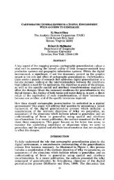
wetlands. Two sets of products, therefore, were generated: 

(1) area measurements and graphics indicating change in 

each subdelta, and (2) area measurements and graphics 

indicating change in the entire delta (Figure 1 and Table 

1). 

Table 1. Comparison of area summaries for the Mississippi 

River Active Delta in 1956 and 1978. 

HABITAT TYPE 

MARSH 

FORESTED WETLAND 

UPLAND 

SPOIL 

1956 

ACREAGE 

182,838 

7,894 

3,362 

3,057 

1978 

ACREAGE 

89,381 

3,233 

6,915 

11,369 

ACREAGE 

CHANGE 

-93,457 

- 4,661 

+ 3,553 

+ 8,313 

°0 CHANGE 

- 51% 

- 59°0 

+ 106°0 

+ 272°0

MISSISSIPPI RIVER ACTIVE DELTA (1956) MISSISSIPPI RIVER ACTIVE DELTA (1978) 

Figure 1. Mississippi River Active Delta as it appeared in 1956 and 1978

Graphic products and reports from this project have not only 

been used by USAGE and USFWS for regional and site-specific 

locational decisions, they have also been presented before 

Parish, State, and Congressional legislative bodies. Prod 

ucts from this project have been presented to the Louisiana 

Senate and House Committee on Natural Resources by Senator 

Samuel B. Nunez, Jr., to highlight and portray the dramatic 

problem of coastal wetland alterations incurred by man's 

activities (Nunez and Sour 1981). Senator Nunez's presen 

tation contained the major graphical display of wetland 

change to the committee. The State of Louisiana later 

allocated $35 million to various State agencies and organi 

zations in an attempt to address the serious problem of 

wetland loss. Other uses of these products have influenced 

similar results, although not as dramatic, at hearings 

before a subcommittee of the House of Representatives in 

Washington, B.C. (Johnston 1981). High quality graphics and 

professional delivery of those products and information, 

therefore, have significantly affected State and Federal 

decisions concerning coastal resources. Products are also 

being used by a number of educational institutions such as 

the Louisiana Nature Center and Louisiana State University. 

Dredge Disposal and Port Development 

The Mobile District U.S. Army Corps of Engineers (USAGE) 

required the use of geoprocessing capabilities to effec 

tively analyze the potential impacts of depositing dredge 

material in coastal areas. The dredge material disposal 

problem arose from the Corps' mandate to deepen Pascagoula 

and Mobile Bay ship channels from 35 to 55 feet deep. NCET 

has constructed a large geographic database consisting of 

wetland and deep water habitats, benthic assemblages, bottom 

sediments, salinity, archeological sites, artificial reefs, 

oyster leases, distribution of 23 species of finfish and 

shellfish, oyster reefs, bathymetry, and current dredge 

disposal sites. The geographic analysis of multiple re 

source overlays are being conducted to select sites for 

dredge disposal and to measure the impacts of fish and 

wildlife resources with disposal actions. This continuing 

program should assist USFWS and USAGE in minimizing the 

impacts of dredge disposal on important marine and estuarine 

resources. Cartographic modeling of the entire Mississippi 

Sound and Mobile Bay is currently being negotiated as an 

additional analysis for delineation of the most sensitive 

offshore biological communities. 

BLM Environmental Impact Statement for Offshore Oil and Gas 

Leasing 

The current administration has opened up vast areas in the 

Gulf of Mexico to oil and gas exploration. The Bureau of 

Land Management's Offshore Continental Shelf Office (now 

Minerals Management Service, MMS) was required to write an 

environmental impact statement on oil and gas exploration 

for the entire Gulf of Mexico. NCET was requested by the 

Assistant Director of the Department of Interior to assist 

MMS in gathering data and calculating areal and linear 

measurements of coastal resources in the gulf. Areal and

linear measurements had to be conducted for a number of 

political and planning unit areas, ranging from the county 

level to extensive offshore planning units. Standard U.S. 

Geological Survey 1:250,000 scale geounits were used as base 

maps for a study area which consisted of the entire Gulf of 

Mexico. Tabular summaries of resource information were 

generated for each county bordering the coast. These 

summaries included the distance or length of shoreline 

features along the coast, including recreational beaches, 

mangroves, marshes, etc. Area summaries were also calcu 

lated for important offshore resources such as seagrass 

beds, nursery grounds, and shellfish concentration areas. 

Each geographic unit, i.e., county, was then ranked in terms 

of resource priority based on these measurements (MMS 1982). 

Oil and gas leases will be given an environmental ranking 

according to their proximity to the areas and the probabil 

ity of an oil spill reaching the most important coastal 

areas. 

A second analysis for the impact statement was conducted for 

scattered areas in the gulf consisting of live bottoms and 

restricted areas where oil and gas activities are limited. 

These restricted areas were delineated according to their 

distance from live bottoms or no activity zones where no oil 

and gas activities are permitted. Zones range from 1 to 

4 miles, with more restrictions enforced in the zones closer 

to live bottom areas. MMS requested the acreages and per 

centage of each oil lease block occupied by the live bottom 

areas and various restricted activity zones. The lease 

blocks and the restricted activity zones were digitized for 

12 areas at a scale of 1:120,000. MOSS was used to generate 

color graphics and area summaries of the intersections 

between the lease blocks and zones (Figure 2 and Table 2). 

MMS used these figures to assign an environmental ranking to 

each block based on the area and percent of each block with 

in the restriction zones (MMS 1982). Quantifying the 

effects of Outer Continental Shelf oil and gas development 

on coastal ecosystems will continue for the next 3 years. 

Table 2. Acreage summaries for lease blocks A367 and A368. 

A 36 7 

A367 

A367 

A368 

A368 

A368 

A 368 

TOTAL 

SUBJECT 

(IN ACRES) 

4 MILE/ZONE 

1 MILE/ZONE 

NO ACTIVITY 

3 MILE/ZONE 

1 MILE/ZONE 

4 MILE/ZONE 

NO ACTIVITY 

AREA 

3491.85 

1973.96 

279.48 

5745.3 

1205.58 

1211.77 

3289.45 

26.93 

FREQUENCY 

1 

1 

3 

5 

1 

1 

1 

1 

PERCENT 

60.78 

34.36 

4.86 

100.00 

21.03 

21.13 

57.37 

TOTAL (IN ACRES) 5733.7 4 100.00 

.47

L KKKFS 

[ J NO ACTIVITY 7X)NKS 

{iiiiiiiiiiiiHll ' MU.K /X>NKS 

[' 1 4 MII.K /ONKS 

I.I.ASK BLOCKS 

5.2 KILOMETER 

Figure 2. Plot of offshore lease blocks in West and East Flower Gardens

Oil Spill Vulnerability Modeling 

A recent pilot project undertaken by NCET for the Louisiana 

Offshore Oil Port (LOOP) produced a composite map depicting 

protection priorities for onshore and nearshore areas in the 

event of an oil or toxic chemical spill. The project demon 

strated the use of MOSS cartographic modeling capabilities 

to indicate the vulnerability of different geographic areas 

to oil and toxic chemical spills. 

The Barataria Pass quadrangle in coastal Louisiana was 

selected for the study area. Inputs for the analysis con 

sisted of eight resource variables: wetland habitats, 

oyster leases, recreational beaches, historical sites, 

endangered species, bird rookeries, marinas, and water 

intakes. These resource variables were ranked from low 

vulnerability (1) to high vulnerability (3). Ranking cri 

teria consisted of a previously developed methodology for 

ranking biological habitats (Ad.ams et al. 1982), and methods 

utilized by the New Orleans MMS office. Resource maps were 

digitized and the all point data were buffered with distance 

factors to indicate zones of proximity to the resource. 

Resource overlays were converted to a cell format and 

receded to the appropriate value determined by the ranking 

criteria cited above. The cell maps were arithmetically 

composited using cartographic modeling methods to produce 

single map indicating oil spill vulnerability. Vulnerabil 

ity index values were grouped into logical classes to pro 

duce a final map product that depicted three levels of 

vulnerability: (1) low vulnerability, (2) medium vulnera 

bility, and (3) high vulnerability. Figure 3 depicts the 

distribution of these values in the Barataria Pass 7%' USGS 

quadrangle. 

Additional work and products will facilitate oil spill 

cleanup activities and deployment of spill response per 

sonnel in order to protect those areas of highest vulner 

ability. Data will be available on NCET's computer system 

with an offsite graphics terminal and in atlas form plotted 

on opaque stable base material. The opaque overlays will be 

overlayed on USGS quadrangle for visual geographic referenc 

ing. This particular application has utility in hazardous 

waste and oil spill management, environmental impact assess 

ments, effluent discharge assessment, and development con 

tingency plans for the cleanup and deployment of spill 

response personnel. 

SUMMARY 

The National Coastal Ecosystems Team is using geoprocessing 

methodologies to assist agencies who have legislative man 

dates or responsibilities to manage coastal resources. The 

above case studies illustrate how NCET's geographic infor 

mation system was and is being used to address a variety of 

coastal issues. These studies are not a complete review of 

applications at NCET; however, they provide a record of the 

types of analyses that are being applied to resource issues 

in coastal and offshore areas using CIS technology. Color 

graphics and tabular summaries produced at NCET have helped

influence important environmental decisions on a variety of 

levels. 

To have significant impacts, these materials had to be 

presented by professional witnesses who were well versed in 

the complexity and problems associated with biological 

systems and who can effectively present facts and conclu 

sions at local, State, and Federal legislative levels. 

In conclusion, if management of coastal ecosystems is to be 

based on the best available information, it is imperative 

that this knowledge be transferred to decisionmakers in a 

form that is readily accessible and understandable. Geo- 

processing techniques at NCET have provided the means for 

accurately analyzing and portraying information for use by 

scientists, administrators, and lawmakers at many levels. 

The result has been a successful rapport between various 

Government officials and a significant impact on coastal 

decisionmaking. 

REFERENCES 

Adams, J.K., K.A. Benkert, C. Keller, and R, White. 1982. 

A Method for Ranking Biological Habitats in Oil Spill 

Response Planning--Louisiana Offshore Oil Port. 

Unpublished report prepared for LOOP, Inc., Harvey, 

LA, by USFWS, Slidell, LA. 

Johnston, J.B. 1981. Hearing testimony presented to the 

Congress of the United States, House of Representatives 

Committee on Merchant Marine and Fisheries, Serial 

No. 97-24, November 20, 1981, Washington, DC, pp. 

265-272. 

Minerals Management Service (MMS). 1982. Draft Regional 

Environmental Impact Statement. MMS Gulf of Mexico 

OCS Region, Metairie, LA. 

Niedzwiadek, H.A., and C.W. Greve. 1979. WAMS: A Computer- 

based Mapping and Data Base Management System, unpub 

lished paper developed for NWI/USFWS, Autometric 

Inc., Falls Church, VA. 

Nunez, S.B., Jr., and A. Sour. 1981. Report on Special 

Projects for Coastal Louisiana. Louisiana Senate and 

House Committees on Natural Resources, October 12, 

1981, Baton Rouge. 

Reed, C. 1980. Habitat Characterization: A Production 

Mode Usage of a Geographic Information System, 

Patricia A. Moore, ed., Computer Mapping of Natural 

Resources and the Environment, Vol. 10, pp. 113-119. 

Laboratory for Computer Graphics and Spatial Analy 

sis, Cambridge, MA.

U.S. Fish and Wildlife Service (USFWS). 1980. Wetland 

Analytical Mapping System User's Manual, unpublished 

paper, U.S. Fish and Wildlife Service, Western Energy 

and Land Use Team, Fort Collins, CO. 

U.S. Fish and Wildlife Service (USFWS). 1982. Map Overlay 

Statistical System User's Manual, draft unpublished 

manual, U.S. Fish and Wildlife Service, Western Energy 

and Land Use Team, Fort Collins, CO.

DIGITAL MAPPING IN A DISTRIBUTED SYSTEM ENVIRONMENT 

Dr. M. Mosaad Allam 

Topographic Survey Division 

Surveys and Mapping Branch 

Department of Energy, Mines and Resources 

615 Booth St., Ottawa 

Canada K1A OE9 

ABSTRACT 

Over the last two decades there has been a gradual advancement of 

digital technology within most mapping organizations, especially in the 

fields of photogrammetric computer mapping and computer-assisted 

cartography, the efficiency of which is greatly influenced by the 

processes of data acquisition, the encoding of various information for 

storage, and the manipulation of data within the system. 

The current trend in system development (hardware, software and 

operation) is directed towards the configuration of sub-systems in a 

distributed computer network. The development of distributed systems is 

a natural outgrowth of the requirements to increase our computational 

abilities and to optimize the sub-systems resources. Even though the 

individual components operate autonomously, the common master data base 

is the unifying element. The configuration of the total system depends 

mainly on the user requirements, the availability of the system to 

various users, the source of digitization (aerial photography, existing 

maps, etc.), the structure of the common topographic/cartographic data 

base, the interaction between the various sub-system components and the 

form of output. 

The functional requirements of distributed digital mapping systems are 

described. The various methods that can be used to achieve the inter 

connection between the various sub-systems, the communication mechanism 

and the characteristics of distributed data bases are also given. 

INTRODUCTION 

The most compelling benefit of digital mapping in a distributed system 

environment is the ability to share information. Distribution means not 

only one program can visit many different processors, but, conversely, 

that one processor and its associated data bases can be accessed by many 

different sub-systems. Time-sharing is not a new idea. Time-sharing 

was developed out of the need to obtain raw computing power at 

reasonable cost, and data sharing was initially viewed as a secondary 

benefit. 

Today, the economics have changed considerably to the extent that raw 

computing power is available at low cost through microprocessors and 

minicomputers thereby reducing the need to share a processor for 

computational power alone. While this suggests that there may be a 

shift in emphasis from time-shared computers to stand-alone dedicated 

systems, the recent trends are directed towards the multicomputer 

configurations, mainly because of the need to share the data bases. 

13

The increase in adapting digital technology in mapping organizations and 

the success achieved in automating the various topographic/ cartographic 

processes, coupled with the desire to optimize sub-systems resources are 

focussing the attention of system designers, managers and users to the 

need for building digital topographic data bases. In large mapping 

organizations, this can be achieved by automating the compilation of 

data base elements in the topographic map production processes. This 

includes the automation of the following functions: data acquisition, 

reduction, indexing, storage/retrieval, computation, analysis, editing, 

data base maintenance/management, and generation of output in digital or 

analog forms. 

To achieve these objectives, it is necessary to design and develop a 

plan from a systems approach which integrates the following various 

functional activities into a unified production system: 

- computer-aided photogramraetric map compilation, 

- digital compilation using automated photogrammetric instruments, 

- graphic digitization (manual, semi-automatic and/or fully auto 

matic digitizing devices), 

- automated cartography, 

- editing and/or digital map revision, 

- generation and manipulation of local data bases by various sub 

systems, according to their functional activity, 

- translation (restructuring) of local data base elements into a 

master data base, 

- graphic output and digital output sub-systems, and 

- etc. 

The analysis of various production sub-systems (activities) clearly 

indicates that a distributed system environment is the most practical 

and efficient methodology to utilize in the system design. 

FUNCTIONAL REQUIREMENTS OF 

DISTRIBUTED DIGITAL MAPPING SYSTEM 

The functional requirements for a digital mapping system in a 

distributed environment can be summarized as follows: 

1. Data Acquisition 

The source material used for the digital compilation of topographic/ 

cartographic products are received in both analog or digital form. In 

the analog form, we find aerial photography and graphic maps, while 

digital sources include scanned aerial photographs or digital imagery 

acquired by airborne solid-state linear array cameras. The essence then 

is to capture the data digitally in order to provide the necessary input 

information for data base manipulation procedures. 

1.1 Digitization from Analog Aerial Photographs 

Computer-aided photogrammetric map compilation using analog aerial 

photography as source is achieved by the interfacing of photogrammetric 

plotters to digital computers. Varius system configurations have been 

successfully developed in numerous mapping organizations. As a prime 

example, we find the multiple-station digital photogrammetric 

compilation systems developed in the Topographical Survey Division, 

Surveys and Mapping Branch, Ottawa, Canada (Allam, 1979). 

14

1.2 Digitization of Existing Graphics 

Graphic sources are existing maps, photogrammetric manuscripts, ortho- 

photo maps, etc., and the process of digitization is regarded as a 

conversion of data records from analog to digital form. This is 

achieved by: 

a) manually retracing the graphic features on a digitizer table with 

a cursor or stylus, 

b) employing a semi-automatic line-following device, or 

c) processing the entire graphic automatically with a raster scanning 

digitizer. 

In the first two methods, the output is a series of X and Y coordinates 

in the digitizer coordinate system. The third method produces a digital 

output in a raster format, which for data purposes requires conversion 

from a raster to a vector format. 

Systems for digitizing existing graphics consist of multiple work 

stations (terminals) for data entry, display, -editing, etc., interfaced 

to a digital computer. 

1.3 Compilation from Digital Imagery 

Digital stereo imagery may be acquired by scanning aerial photographs on 

automated photogrammetric instruments or in real-time by means of 

airborne linear array cameras. The compilation of topographic detail 

requires an automatic correlation (matching) of the conjugate digital 

stereo-imagery, while the compilation of planimetric detail requires a 

solution of the complex problems of digital image analysis and pattern 

recognition. This mode of compilation is heavily dependent on 

processing using digital computers. 

2. Data Storage and Retrieval 

Depending on the mode of data acquisition, the data is stored in a 

retrieval format in the sub-systems local data base. To build a master 

digital data base, the data is restructured according to a standardized 

digital data base, also in a retrievable format. The stored data must 

include positional coordinates and sufficient description information to 

make it useful across a spectrum of digital mapping products. In 

addition, they are stored at a resolution capable of supporting the 

majority of the products. 

3. Data Manipulation 

When a specific product is requested, the data contained in the master 

data base (or local data base) within the geographic area of interest is 

extracted and is used as input to the digitial manipulation process. 

This function requires several user dependent operations, and includes: 

- selection of specific feature types, 

- display of digital data, 

- cartographic editing and enhancement, 

- data compression, 

- projection adjustment and transformations, 

15

- mathematical processing/restructuring (e.g. generation of digital 

elevation models - DEM's), 

- symbolization, 

- statistical analysis, 

- report generation, etc. 

The output of the process may be a digital file structured according to 

a standardized digital exchange format or a digital file that can be 

used to drive a finishing device. 

4. Graphic Output 

This function entails the use of the digital data desired to produce the 

necessary map/chart overlays using automatic plotting/scribing devices. 

This function also includes a quality control task and other manual 

processes as required. 

In addition to these four basic tasks a digital mapping system in a 

distributed computer network will support other functions such as: 

- resource sharing 

- system management and control 

- batch processing and program development 

- multiple user defined data base inquiry operations 

DEVELOPMENT OF DISTRIBUTED DIGITAL MAPPING SYSTEM 

A distributed system is achieved by interconnecting the computers of the 

digital mapping sub-systems in a manner that provides optimum 

interchange of digital data between the various sub-systems, in addition 

to the interchange of data between the various terminals, graphic work 

stations and peripherals within each sub-system. In essence, the 

development of a distributed digital mapping system may be regarded as a 

computer network including hosts (central) computers, nodes 

(minicomputers), terminals (work stations, digitizers, video terminal, 

graphic editing stations, etc.), and transmission links. 

A host in this context is a central computer whose function is separate 

from that of switching data. A node is a computer that primarily is 

only a switch. Some designs permit a computer to be both node and host. 

Terminals are interface between the user and computer network. Trans 

mission links join the hosts, nodes and terminals together to form a 

network. A path is a series of end-to-end links that establishes a 

route across part of the network. The links and nodes along with the 

essential control, make up the communication sub-net, or the digital 

mapping data network. 

Classification Schemes of Distributed Systems 

Network topology, as a mean for categorizing digital data communication 

networks evolved from graph theory (Deo, 1974). Terms borrowed from 

graph theory include the previously defined host, node, link and path. 

This terminology forms the basis for topological classification of data 

networks as follows: 

16

1. Centralized Network 

It is essentially a star configuration (links radiating from a single 

node), is the simplest arrangement, as shown in Figure 1. This topo- 

logical scheme requires a link to be dedicated between the central 

computer (node) and each terminal. This type of configuration is 

normally found in digital mapping sub-systems dedicated for one 

activity, e.g. computer-aided photogrammetric compilation. The reliabi 

lity of the centralized network depends on the central computer (node). 

Its failure suspends all activity in the network, whereas individual 

link failures affect only a single device per link. 

2. Centralized Network with Concentrators/Multiplexers 

Where several terminals in a geographically dispersed system are close 

to one another, they are often connected to concentrators or multi 

plexers, which in turn are connected to the central computer as shown in 

Figure 2. The devices (normally microprocessors) obtain more efficient 

link utilization at the expense of an occasional delay in response time. 

A multiplexer is used where the information transfer rate of all 

simultaneously active terminals never exceeds the information transfer 

capacity of the link to the central node; but where the potential input 

capacity exceeds link capacity a concentrator is necessary because of 

its storage capacity. Concentrators can also merge several low-speed 

links into one high-speed link. However, concentrators and multi 

plexers cannot save a network when the central node fails. 

3. Decentralized Networks 

As shown in Figure 3, a decentralized network is an expanded centralized 

configuration with the concentrators/multiplexers replaced with mini 

computers or microcomputers (nodes), having more memory and storage 

capacity. The added reliability of decentralized processing power comes 

at the expense of additional computers (nodes) and corresponding 

connecting links which permit some paths to be duplicated. Within 

reason, the reliability of the network can be increased almost 

indifinitely by duplicating paths and adding links and nodes. 

4. Distributed Networks 

As shown in Figure 4, a distributed network is similar to the decen 

tralized configuration, but with each node connected to at least two 

other nodes in mesh form. A single ring is the simplest form, with each 

node connected exactly to the two other nodes. Each node can switch 

systematically between links according to a routing algorithm, to 

maximize the capacity of the network. 

Distributed networks could be designed with a homogeneous structure, 

that is identical hardware at each node or hierarchical. In hierar 

chical configuration, there exists several sub-nets connected to one or 

more nodes. This hierarchy will allow for the use of various types of 

computers with varying power and function at each level and the backbone 

processor of such a system configuration is designated for the master 

data base. This type of hierarchical form makes it difficult to differ 

entiate between the decentralized network structure and the distributed 

network and presently most designers can no longer distinguish between 

the two classes. 

17

Concentrators, 

Multiplexers 

Link 

Figure 1 Centralized Network 

Figure 2 Centralized Network with 

•Terminals 

Central Computer 

Concentrators / Multiplexers 

18 

Central 

Computer

Figure 3 Decentralized Network 

Computer 

(Nodes) 

Figure 4 Distributed Network 

19 

Link

COMMUNICATION AND NETWORKING 

As shown in Figure 5, it would be a relatively straightforward task to 

design and build a communication mechanism whereby two programs, 

residing in the same computer, can send information or messages to each 

other. This is what is commonly known as interprocess communication 

facilities in operating systems. 

In a distributed system the communication between programs reside in 

separate processors and hence a distributed communication mechanism must 

be created. Two halves of a single mechanism or service must 

communicate and synchronize to perform a unified function. This 

communication is used not only to pass information between the systems 

but also to pass control information between the communication mechanism 

programs themselves. For that, a communication protocol is needed and 

is the only connection between the two distributed parts as shown in 

Figure 6. 

Software is needed to enable multiple digital computers to be inter 

connected. This software is normally implemented as a set of layered 

network protocols, each of which is designed to fulfill specific 

functions whithin the network. 

Software for each digital mapping sub-system activity, whether a data 

acquisition sub-system(s), data manipulation sub-system, data base sub 

system or output sub-system, will be implemented as application 

software. This software must be designed and developed to achieve a 

synchronization of the system activity across multiple processors with 

the objective of sharing local data bases within each sub-system and the 

master data base containing the central data files. 

DISTRIBUTED DATA BASES 

The successful implementation of many distributed systems requires 

solutions to problems of data management in a distributed environment. 

These problems include data collection, concurrency control and update 

processing, failure recovery, and query processing. 

In a distributed digital mapping system, data collection is fulfilled by 

the data acquisition sub-systems, and creation of local data bases. To 

collect the data in a central (master) data base, translation programs 

are necessary to reformat the files according to a standardized data 

base structure. 

The coordination of concurrent updates initiated by multiple users must 

be done in a way that preserves the consistency of the data base. 

Updating should be made according to a data base manager program which 

acts on updates based on their sequence and/or time of requests. 

Distributed system should have a failure recovery mechanism allowing the 

system to operate in a resilient manner and preserving the integrity of 

the data base. Ideally the system should continue functioning, although 

perhaps in a degraded mode. 

20

I 

N 

T 

E 

R 

F 

A 

C 

DIGITAL 

COMPUTER 

Figure 5 Local or Centralized Communication Mechanism 

DIGITAL 

COMPUTER 

LOCAL 

STORAGE 

COMMUNICATION 

MECHANISM 

Physical 

Media 

DIGITAL 

COMPUTER 

1 1 1 

LOCAL 

STORAGE 

Figure 6 Distributed Communication Mechanism 

21 

nr N 

T 

E 

R 

F 

A 

C 

-USER 

B

Locating stored data in a distributed system will be simplified if the 

data is translated and transferred from the local data bases, in each 

digital mapping sub-system, to the master data base. If this is not the 

case, the distributed system program must determine where the data 

required by a query is stored. This problem can be solved by using a 

distributed data base management system, which allows the data to be 

sorted at multiple locations in the network and yet accessed as a single 

unified data base. 

In a digital mapping environment, the approach of constructing a central 

data base from local data bases generated by various sub-systems will be 

preferred, due to the need for the exchange of digital map data among 

various organization/users, not directly linked to the distributed 

digital mapping system. 

CONCLUSION 

Distributed data processing systems are a new class of organizations and 

operations that exhibit a high degree of distribution in all dimensions, 

as well as a high degree of cooperative autonomy in their overall 

operation and interaction. By interconnecting the digital computers 

controlling various digital mapping sub-systems in a distributed 

environment, large mapping organizations will benefit from the improved 

performance, improved system availability, easier adjustment to a 

growing workload, extended control over computer resources, and the 

advantage of master digital data base. The dramatic drop in the cost of 

computers versus the increased cost of software and computer personnel 

makes distributed systems inevitable. 

REFERENCES 

1. Allam, M.M., 1979, Multiple Station Interactive Map Compilation with 

Distributive Computer Network, Proceeding Auto Carto IV, Reston, 

Virginia, November 1979, PP. 379-404. 

2. Deo, N., 1974, Graph Theory with Applications to Engineering and 

Computer Science, Englewood Cliffs, N.J., Prentice-Hall, 1974. 

22

AN OVERVIEW OF DIGITAL ELEVATION MODEL PRODUCTION 

AT THE UNITED STATES GEOLOGICAL SURVEY 

W.R. Allder 

V.M. Caruso 

R.A. Pearsall 

M.I. Troup 

United States Geological Survey 

National Mapping Division 

National Center, MS 510 

Reston, Virginia 22092 

ABSTRACT 

The U.S. Geological Survey (USGS), through the National 

Mapping Program (NMP), has the objective of preparing and 

making available multipurpose maps and fundamental carto 

graphic and geographic information to meet the diverse 

requirements of users throughout the nation. The NMP con 

centrates on gathering those base categories of data 

depicted on topographic maps. There is an inherent relation 

ship between two of these categories: orthophotographic 

imagery and hypsography. The National Mapping Division (NMD) 

of the USGS has been producing standard orthophoto products 

from high-altitude aerial photographs using automated 

orthophoto equipment since the mid-1970's. Byproducts of 

this operation are arrays of digital elevations that can be 

post-processed into digital elevation models (DEM's). Data 

collection techniques and constraints, while not affecting 

the quality of the orthophoto imagery, may impact the 

geomorphic fidelity of the digital terrain byproduct. This 

paper describes the collection of DEM data by the NMD, the 

means by which data errors are introduced and identified, 

and the editing techniques that may be employed to improve 

the quality of DEM's to meet user requirements. 

INTRODUCTION 

History 

In the 1970's, two efforts within the NMD (then Topographic 

Division) of the USGS converged to create the digital 

elevation model (DEM) production system as it exists today. 

H Since the mid-1960's, increasing user acceptance of 

and demand for orthophoto products had spurred efforts 

to develop a means of using digital input data to 

control automated operation of the T-61 and T-64 

Orthophotoscopes. The use of digital profile data to 

control the z-motion of the exposing projector of the 

orthophotoscope was seen as a means to both increase 

production and improve image quality. This effort 

Any use of trade names and trademarks in this publication is 

for descriptive purposes only and does not constitute 

endorsement by the U.S. Geological Survey. 

23

culminated in the development of the Digital Profile 

Recording and Output System (DPROS), which records 

digital profiles on magnetic tape in a format that can 

be used to produce DEMs as well as orthophotographs 

(Lemeshewsky and Shope, 1977). 

18 In 1974, a growing recognition of the potential use of 

cartographic data in digital form led to the 

initiation of a formal requirements study to define a 

digital cartographic data base to supplement the 

topographic mapping program (Office of Research and 

Technical Standards, 1975). Serving as input to this 

study was a cooperative research project in which NMD 

agreed to furnish terrain elevations and planimetric 

data in digital form to the Geologic Division, USGS 

for use in a computerized Coal Resources Information 

System (Elassal, 1975). One conclusion of this 

project was that the most cost-effective means then 

available for obtaining digital elevation data was the 

recording of profiles from stereomodels (Branch of 

Cartography, 1976). 

In 1977, the study efforts came together when the National 

Mapping Division established a Digital Applications Team 

(DAT) to develop a capability to produce digital carto 

graphic data as a standard product of the National Mapping 

Program. Some digital profile data sets, generated as a 

byproduct of orthophoto production, were already available. 

These data sets were stored in the regional office in which 

they were collected. In addition, the Division in 1976 

procured an automated image correlation system, the Gestalt 

PhotoMapper II (GPM2), to produce slope-corrected ortho- 

photos. Like the manual profilers, the GPM2 is capable of 

generating digital elevation data. Raw elevation data sets, 

generated by the GPM2 during the production of orthophotos, 

were also stored. The DAT developed formats and standards 

for the classification of DEM data which were adopted for 

internal use by the Division. As a result, starting in 1979, 

the raw elevation data sets have been processed into the 

NMD's standard digital elevation model format (U. S. 

Geological Survey, 1980). 

DEM Organization 

"Digital elevation model" (DEM) is the terminology adopted 

by the USGS to describe terrain elevation data sets in 

digital form. A standard DEM has the following 

characteristics (U. S. Geological Survey, 1980): 

H It consists of a regular array of elevations cast on 

the Universal Transverse Mercator (UTM) coordinate 

system. 

0 The data are stored as profiles in which the spacing 

of the elevations along and between each profile is 

30 meters. 

I The unit of coverage is the 7.5-minute quadrangle; no 

overedge coverage is provided. 

B Not all profiles have the same number of elevations. 

24

B It contains approximately 138,000 (at 50 N. latitude) 

to 195,000 (at 25 N. latitude) elevation points. 

The DEM's are classified into three levels according to the 

quality of the model: 

B Level 1-- Raw elevation data sets in a standardized 

format. Only gross errors in data capture have been 

eliminated. 

I Level 2-- Elevation data sets that have been smoothed 

for consistency and edited to remove random errors. 

B Level 3-- Elevation data sets that have been edited 

and modified to insure positional consistency with 

planimetric data categories such as hydrography and 

transportation. 

Virtually all of the DEM's produced to date are considered 

to be level 1 (McEwen and Jacknow, 1979; McEwen and 

Calkins,1981). 

Digital Cartographic Data Base 

To satisfy requirements of the National Mapping Program, the 

NMD is building a Digital Cartographic Data Base (DCDB) 

containing certain base categories of cartographic and 

geographic data. The DCDB consists of eight sublevel data 

bases which allow the digital cartographic data archived on 

magnetic tape to be indexed in several ways. One of the 

types of cartographic data indexed in this manner is the 

DEM. The DCDB currently manages in excess of 7,500 DEM's. 

Of this number, 70 percent were produced from raw data 

generated using GPM2 equipment. The GPM2 instruments have 

been used primarily to produce orthophotos in mountainous 

areas in support of Federal land and resource management 

agencies (McEwen and Jacknow, 1979). This is reflected in 

the present contents of the data base (See fig. 1 ). 

DEM's in the DCDB are stored in one of two sublevel data 

bases as determined by the tested vertical accuracy: less 

than 7 meters vertical root mean square error (RMSE); and 7 

to 15 meters vertical RMSE. The 7 meter RMSE was determined 

to be a reasonable standard for DEM's derived from 40,000 

foot high-altitude aerial photographs, attainable under a 

variety of terrain conditions and instrument constraints 

(Brunson and Olsen, 1978). Less accurate data sets are 

retained if they are the best available. 

COLLECTION 

To meet present user requirements for DEM production, the 

National Mapping Division uses three systems to collect the 

digital elevation data. They are (1) the Gestalt PhotoMapper 

II (GPM2), (2) manual profiling from stereomodels, and (3) 

the Digital Cartographic Software System (DCASS). 

The GPM2 is a highly automated photogrammetric system 

designed to produce orthophotos, digital terrain data, and 

photographic contours. An electronic image correlation 

component of the GPM2 measures parallaxes of 2,444 points 

25

FIGURE 1: 

CONTENTS OF DEM DATA BASE 

COVERAGE AS OF 8/1/32

within each 9- x 8- millimeter area of a photogrammetric 

stereomodel.Of these 2,444 correlated points, subunits of 

576, 1,024, or 1,600 points are collected for inclusion in 

the elevation model. These subunits are called "patches" and 

the patch size is selected to accommodate various terrain 

conditions. The horizontal (x and y) resolution of the 

elevation points within each patch is approximately 182 

micrometers at photo scale (a ground distance of 47 feet 

when using high-altitude photography at 1 :80,000-scale). 

Each of the two stereomodels covering a standard 7.5-minute 

quadrangle contains over 500,000 correlated points, which 

are regridded to form a DEM in the standard DCDB format. 

The manual profiling systems use stereoplotters, interfaced 

with electronic digital profile recording modules, for 

scanning of stereomodels in the photo y direction. Image- 

density-controlled high-altitude aerial photographs are used 

as source material. The scan speed and slot size (stepover 

interval) can be varied by the operator to accommodate 

differential changes in topographic slope. A 4- millemeter 

slot size is most commonly used; thus profiles are spaced 

approximately 300 feet apart. Elevations are normally 

recorded every 100 feet along each profile. The raw 

elevation data are reformatted and regridded to the standard 

DCDB format and tested for vertical accuracy before place 

ment in the DCDB. The primary use of the digital profile 

data is to drive a WILD OR-1 or Gigas-Zeiss GZ-1 to produce 

an orthophoto. 

Lastly, DCASS forms a DEM from digitally-encoded vector 

contour data. Stereoplotters, interfaced with three-axis 

digital recording modules, are used to collect vector 

contour data while the instruments are being used for 

1:24000-scale photogrammetric stereocompilation. During the 

acquisition phase, the contours are assigned elevation 

values (attributes). The vector contour data are processed 

into scan lines and the elevation matrix is formed using a 

bilinear interpolation between the intersections of scan 

lines with the contour vectors. DCASS was initially 

developed to perform automated map compilation. Its primary 

goal is to produce color separates for map reproduction. 

The methods used for determining vertical accuracy differ 

with the collection method. With the GPM2, an RMSE value is 

derived from a weighted solution of the relative elevation 

differences between extrapolated patch joins and the rela 

tive elevation difference between coincident points in the 

overlap area of the two stereomodels covering a quadrangle. 

The RMSE of the elevation data derived from the manual 

profiling and DCASS systems, however, is computed by 

comparing known ground vertical control elevations for a 

minimum of ten (10) discrete image points to the linearly 

interpolated DEM elevation points. 

ERROR DETECTION AND VERIFICATION 

Most elevation errors are introduced during the data acqui 

sition phase. Depending upon the particular recording device 

and the operating procedures that are used for data capture, 

elevation errors may be introduced into the DEM data in a 

27

variety of ways. 

The GPM2 uses an automated image correlation technique to 

accomplish stereorestitution, and there are natural terrain 

conditions under which the correlator cannot derive precise 

elevations. Additionally, the ground resolution of the 

elevation data from the GPM2 is finer than the resolution of 

the resampled data within the NDCDB, and the subsequent 

regridding, interpolating, and smoothing of the data tends 

to generalize the terrain topology. 

The manual profiling technique of orthophoto generation uses 

procedures that may introduce DEM elevation.errors in 

another manner. The width of the scanning slot, and the 

associated digital profile spacing, is typically larger than 

the sampling interval along profiles. This disparity in the 

bidirectional ground spacing of elevation data, while 

justified in terms of time requirements and orthophoto image 

quality, causes loss of topologic detail. Local features 

falling between scan lines will not be represented. 

Another area where errors can be introduced when using the 

manual profiling technique is associated with the instrument 

operator. In profiling, the operator must manually keep the 

"floating dot" on the surface of the stereomodel. Optometric 

studies indicate that there is systematic operator tendency 

to profile above ground level while scanning downhill, and 

below ground level while scanning uphill. The normal data 

collection procedure of alternating the profile direction 

thus tends to introduce an alternating data error. Graphics 

produced from this data exhibit a herringbone pattern, 

particularly in steep terrain (Brunson and Olsen, 1978). The 

operator's reaction time to differential changes in slope 

and natural terrain features may also introduce incorrect 

elevation values. The elevation data from the manual 

profiling systems tend to be more generalized then the GPM2 

data, due to the higher degree of operator generalization of 

the terrain during the recording process and the sparser 

sampling intervals. 

With DCASS, vector contours are compiled by use of standard 

photogrammetric map compilation practices, and elevation 

grids are then derived from the contours. Therefore, the 

accuracy of the DEM data is dependent on the cartographer's 

ability to accurately define the contours and the gridding 

algorithm that is used to convert the contours to an 

elevation matrix. Vertical accuracy tests using 90 to 220 

points per quadrangle yield average elevation errors of less 

than one-half the contour interval (Boyko, 1982). 

In all the above data acquisition systems, the photogram- 

metric procedures that are used in establishing control 

necessary for a proper orientation of the models to the 

ground may introduce errors or distortions into the DEM. The 

proper interior, relative, and absolute orientations are 

necessary in order to minimize errors in model elevation 

datum and scale. 

The current NMD collection techniques do not constrain OEM's 

to known planimetric topographic features such as ridge- 

28

lines, water courses, and transportation networks. The 

geomorphic fidelity of these features is many times 

distorted or possibly lost due to either the raw data 

collection interval or the flattening effects of subsequent 

interpolation.No matter which DEM production procedure is 

used, elevation errors, if uncorrected, result in DEM's that 

are physically incorrect portrayals of the terrain surface. 

Quality control procedures for detection and verification of 

errors have been developed which cover many phases of data 

production, from initial data collection to public distri 

bution. The most common forms of quality control procedures 

make use of diagnostic programs and verification graphics at 

various checkpoints within the production processes. These 

include isometric and contour plots, color image displays, 

and programs which output error logs or symbol-encoded error 

plots. 

Verification graphics derived from DEM data can be used for 

a visual comparison with existing forms of line manu 

scripts. User-supplied transformation parameters, in the 

form of desired geographic projection, plotting scales, 

viewing angles, and map coordinate bounds, are used in 

conjunction with the DEM data to produce verification 

graphics. Plotting hardware includes electrostatic printers, 

pen plotters, and cathode ray tube display devices. 

Detection techniques which use diagnostic printouts and 

error symbol plots have evolved as cost effective methods. 

NMD is currently developing another method of DEM quality 

control which makes use of a color image-display system to 

accentuate certain types of error signatures by color 

banding, shaded relief, and anaglyphic stereo. This type of 

quality control is being used on a developmental basis to 

check data files input to and output from NMD digital data 

bases. Ultimately, it will be used to preview, and possibly 

edit, DEM data prior to data base entry and (or) distri 

bution. 

EDITING 

At NMD, DEM data can be edited at two stages within the 

production network: the raw data acquisition stage, and the 

regridded DCDB stage. The decision to edit a DEM is based on 

two criteria: (1) the model is observed to contain a 

significant amount of topographic discontinuities (steep 

slopes, water, etc.); or (2) the regridded DEM is found to 

have a large RMSE value. To prevent distortion of the DEM, 

the data should be edited at the input stage and not after 

the data have been regridded to a coarser resolution than 

that collected. However, due to the large volume of data 

contained in raw GPM2 models, this is not always the most 

cost effective approach. 

Because the GPM2 has been the primary source of the USGS 

DEM's the concentration of effort has been directed toward 

development of techniques to edit the raw elevation data 

produced by the GPM2. The GPM2 uses an automated stereoimage 

correlation technique to derive terrain elevation values. 

Perfect image correlation is not always possible due to a 

29

number of factors. The presence of such features as steep 

terrain (cliffs and overhangs), shadows, forests, ice and 

snow fields, and water bodies can cause the GPM2 to obtain 

incorrect elevation values. 

While the GPM2 cannot always derive correct elevations over 

certain types of topographic featur'es, the correlation of 

water areas presents the most significant problem. This 

problem is encountered when the GPM2 is attempting to 

correlate images of water bodies and other terrain features 

where corresponding image points cannot be found. Conse 

quently erroneous elevation values are often assigned to 

grid points that fall within water boundaries. The result is 

a physically incorrect representation of the terrain sur 

face. Software has been developed to modify OEM's that have 

water bodies. The DEM can be modified spatially by pro 

cessing the digital elevation data through this DEM water 

edit software to replace the erroneous elevations with an 

externally derived value for the water surface. A DEM 

containing a significant amount of water coverage will often 

have a large RMSE value. A number of OEM's have been 

modified with this software to date, and the RMSE of each 

has been reduced significantly to permit the DEM to be 

entered into the DCDB (Troup, 1982). 

Various types of mathematical filters may be applied to edit 

OEM's. Experience indicates that such filters, when applied 

to the DCDB DEM files, can remove certain types of errors up 

to a threshold of ± 8 meters without impacting the overall 

accuracy of the model. Discontinuities exceeding that 

threshold are evidence of possible errors in correlation due 

to image quality or terrain conditions that must be 

addressed at the raw data stage. For example, residuals 

derived from GPM2 elevation data are known to be greater 

along patch edges than inside patches (Allam, 1978). These 

residuals affect patch and model joins and are detectable 

in the final regridded OEM's as sudden changes in elevations 

parallel to the x and y axes of the patch data. 

Another type of error detection and correction software was 

developed to determine errors in GPM2 generated elevations 

at the raw data stage (Computer Sciences Corporation, 1978). 

Elevations within each patch are intrarelated due to 

smoothing performed by the electronic and optical systems of 

the GPM2 (Collins, 1981). Each patch, however, is generated 

independently. The error detection software therefore 

considers each patch as a single entity which is analyzed 

with respect to its neighboring patches. The terrain data 

are assumed to represent a smoothly varying surface, i.e., 

the transition between patches should not be abrupt. The 

detection software applies several statistical tests, e.g., 

mean difference and slope and intercept, to evaluate patch 

joins and flag discontinuities in the surface. The test 

results, considered as a whole, provide an indication of the 

types of edits that can be made to improve the model. The 

error correction software also operates on entire patches. 

It permits raising or lowering and tipping or tilting of 

patches to bring them into better conformance with the 

surrounding terrain. Determining the proper corrective 

actions is a complex process requiring the use of subjective 

30

judgment on the part of the editor. Examination and inter 

pretation of the source photography, orthophotoprint, or 

existing published line map can help in this decisionmaking 

process (Computer Sciences Corporation, 1978). 

CONCLUSION 

DEM production at the USGS has evolved from the orthophoto- 

mapping program. The orthophoto and DEM programs are tightly 

coupled, as reflected by project authorizations. Currently, 

there are three elevation data acquisition systems in use 

by the NMD. The primary product of two of these systems, the 

GPM2 and manual profiling, is an orthophotograph. The third 

system, DCASS, was developed to automate the map 

compilation process; its primary product is a set of final 

color separates. In all three cases, DEM's are derivative 

byproducts. 

Raw elevation data sets which are generated by NMD are 

validated using a variety of graphics and diagnostic pro 

grams that are designed primarily to detect gross errors. 

DEM data can be edited or smoothed at several stages in the 

production cycle. Currently, the only edits which are 

routinely performed involve the correction of water sur 

faces and the removal of gross errors. Raw elevation data 

sets are post-processed into a standard format, tested for 

vertical accuracy, and archived in the DCDB. 

DEM's are separated by the NMD into three levels. Virtually 

all of the DEM's which have been collected to date are 

considered to be level 1 because of the limited amount of 

editing performed. A long-term goal of the National Mapping 

Program is to provide digital cartographic data commensurate 

with the inherent accuracy of the 1:24,000-scale topographic 

maps. DEM's produced to the current standards (7-meter 

vertical RMSE) from high-altiitude photographs will not 

satisfy vertical National Map Accuracy Standards for contour 

intervals of less than 80 feet.* Therefore, the data 

currently resident in the DEM data base must be viewed as an 

interim product. 

The USGS has archived thousands of stable-base film positive 

contour separates, and long-term expectations are to 

produce DEM's from automated sensing, measurement, classi 

fication, and processing of the data contained in these 

manuscripts. Currently, NMD is developing a system to 

produce DEM data from the contour separates using automated 

techniques. This in-house system is anticipated to be in 

production by the mid-1980's. These methods are expected to 

produce level 2 data directly. The production of level 3 

data is considered a desirable end goal, and will be 

developed in the future. 

*Based on statistics, the contour interval that can be 

achieved from a given set of data is 3.3 times the RMSE of 

that data, i.e., a 7 meter RMSE is roughly equivalent to an 

80 foot contour interval. 

31

REFERENCES 

Allam, M.M., 1978, DTM's Application in Topographic Mapping: 

Pho tog r

THE COLLECTION AND ANALYSIS OF NATURAL RESOURCE DATA 

IN THE 1980s 

Doyle G. Fredrick 

and 

K. Eric Anderson 

U.S. Geological Survey 

102 National Center 


ABSTRACT 

In an era of increasing need for the discovery and 

development of our natural resources, the U.S. Geological 

Survey has an important role to play. The accomplishment 

of this role will require improved efficiencies in the 

storage, manipulation, and presentation of data, but that 

task will be complicated by current personnel and budget 

constraints. Increasing reliance upon technological 

innovations, therefore, will be essential. The Survey is 

already providing topographic map information in digital 

form and exploring means of automating more of the mapping 

process. Computer modeling has become a common tool of 

Survey geologists and hydrologists. Now these scientists 

are working with Survey cartographers to combine data 

bases in order to efficiently produce comprehensive 

compilations of earth science data. The use of computer 

graphics in all forms has also increased and is now 

commonly used for the analysis and presentation of data 

required in policy decisions. Because the Survey antici 

pates an increasing demand for natural resource informa 

tion in the future and recognizes the many advantages of 

recent technical advances, increased emphasis will be 

placed on the use of telecommunications, automated data 

collection, computer-based analysis, computer graphics, 

and automated mapping in the remaining years of this 

decade. 

INTRODUCTION 

The United States faces many difficult resource and land 

management issues involving: energy and mineral explora 

tion and prudent development, assessment of the Nation's 

water resources (quality and quantity), and natural hazards 

examination, among others. Maps and mapping have always 

played an important role in dealing with issues of this 

type and will continue to serve in a vital capacity in the 

future. As we near the end of this century, several 

problems face the mapmaker, the earth scientist, and the 

land manager who would meet the challenges of providing 

data in these vital areas: 

Location of undiscovered resources requires the 

application of sophisticated techniques commonly 

requiring the processing of large amounts of data. 

33

Also, this will require a look at lands that are not 

altogether accessible wilderness areas, OCS, etc. 

Increasing competition for, and public discussion 

about, the most appropriate use of land and 

resources require detailed consideration of the 

economic and environmental impacts of proposed 

actions, i.e., to leave open for exploration and 

development or set aside. 

Concern about the consequences of action or lack of 

action requires that analysis be done completely 

and quickly. This necessitates extensive modeling 

of natural process and proposed action. Fortu 

nately, technology has now provided the scientists 

and the decisionmaker with a vast array of powerful 

tools to aid the process considerably. 

U.S. GEOLOGICAL SURVEY ROLE 

In order to provide a framework for a discussion related 

to management of natural resource data and the application 

of computer data bases and automated cartography, it might 

be helpful to review briefly the mission of the Geological 

Survey. 

The Geological Survey was established in 1879 and charged 

with the responsibility for the "classification of public 

lands and examination of the geological structure, mineral 

resources, and products of the national domain." Over the 

years the evolution of the earth sciences, the need to 

carefully manage the Nation's nonrenewable resources and 

to find new sources of critical energy and mineral com 

modities, and mounting concern over man's impact on the 

environment have added numerous other duties including 

geographic research, hazards duties, topographic and 

geologic mapping, and water resources assessments. The 

Survey is an impartial research agency that gathers, 

interprets, and distributes data in order to advance 

scientific knowledge of the Earth so that managerial 

decisions related to natural resources can be based on 

objective information. 

To meet the ever increasing needs for the more sophisti 

cated uses of our data, scientists at the Geological 

Survey are embracing computer assisted cartography as an 

essential element of their work. Also, sophisticated 

computer analysis is becoming a common practice among 

those who use our information (inside the Geological 

Survey as well as outside). 

As the primary Federal earth science, research, and fact- 

gathering agency, the Geological Survey provides informa 

tion for sound planning and decisionmaking as it has for 

many years. Now much of that information is provided on 

computer tapes. The computer data bases of the Survey 

must meet the needs of many as a source of information and 

to support analysis, and the cartographic data base should 

also provide the connecting link to permit the integration 

34

of many disparate data sets. In addition, as a major 

mapping agency we must assure that data bases can be used 

to enhance our capability and capacity to prepare and 

revise maps. 

THE CHALLENGE OF THE 1980's 

As both a producer and a user of cartographic and earth 

science data, the Geological Survey, like many other 

agencies, faces major challenges to establish and manage 

these data base and to develop standards to allow easy 

access and convenient use. Already, there are large data 

bases in existence and more are on the way. In addition, 

we are not the only organization to collect and store data. 

To assure that the cartographic, geologic, hydrologic, and 

other related information can be readily used to produce 

comprehensive insights required by today's researchers and 

decisionmakers, the Geological Survey and other mapping 

organizations are obligated to insure that high standards 

of accuracy and integrity are maintained in the design, 

development, and management of these data bases. We must 

provide: the basic foundation to enable the integration 

of many data types and sources, and truly multiple purpose 

data bases that will serve all. 

In recognization of our obligations in these areas, we 

have set out to: 

Manage our internal data bases in a consistent, but 

not oppressive, way. We may now have as many as 

250 separate data bases which require some over 

sight. We have had a Data Base Administrator for 

some time, and a great deal of progress has been 

made. We are now reorganizing our computer opera 

tions to insure additional oversight for the 

Bureau's information systems. 

Develop standards for earth science information 

that can be used both internally as well as 

externally. 

The Geological Survey is carrying out a leadership 

role in the development of standards for earth 

science data through a memorandum of understanding 

with the Bureau of Standards. This is especially 

appropriate considering the Survey's role as the 

Nation's mapper, which provides that core carto 

graphic data set to which all others must tie. 

Committees have been established within the Survey 

and the Department of the Interior to examine and 

review current activities and develop recommenda 

tions to the Bureau of Standards for Federal 

standards on earth science data. The first set of 

standards to go through this process have just been 

published as Circular 878-A: Codes for the 

Identification of Hydrologic Units in the United 

States and the Caribbean Outlying Areas. In 

addition, the Survey has supported the establishment 

35

of a National Committee on Digital Cartographic 

Standards under the auspices of the American 

Congress on Surveying and Mapping. These 

activities represent the beginning stages of an 

ongoing effort to provide the necessary foundation 

to insure the usefulness and applicability of 

automated earth science data now and in the future, 

None of us has the power to legislate standards-- 

hopefully we can be convincing regarding the 

benefits. 

Properly design the data base to assure multi 

purpose use. 

Insure user input into all decisions related to 

data input, etc. 

DATA BASES (EXAMPLES) 

Digital Cartographic Data-. 

Recognizing the essential role of cartographic data for 

resource studies and considering our responsibilities as 

the civilian land mapping organization, we have undertaken 

the development of a national digital cartographic data 

base. This activity encompasses all of the complexities, 

concerns, and obligations discussed earlier. To serve 

national needs, we must insure that our data base: 

Provides data that people need. 

Interfaces with almost every data bases around 

(proved the link). 

Contains enough information for complete analysis. 

Is easily accessible. 

Can be developed at a reasonable cost. 

Accommodates data from others. 

Support the mapping process. 

The National Digital Cartographic Data Base encoinpassses 

planimetric and elevation data from the standard topo 

graphic maps of the Survey. The principal categories of 

planimetric data being included are: the Public Land 

Survey System; county, State, and Federal boundaries, 

highways, roads, trails, and rivers, streams, and water 

bodies. The primary scale of collection is 1:24,000, but 

pilot projects are examining the efficiency of data 

collection at other scales. Elevation data are being 

collected at 1:24,000-scale, but the Survey is also 

distributing elevation data at 1:250,000-scale collected 

by the Defense Mapping Agency. One of the most notable 

achievements of the Survey's digital cartography program 

is the completion of a national series of maps at 

1:2,000,000-scale. 

In response to the need for digital cartographic data 

suitable for applications at regional or national scales, 

the Survey has introduced a data base at the 1:2,000,000- 

scale. This data base was constructed from the general 

reference maps of The National Atlas of the United States 

36

of America. It includes political boundaries (State and 

county level), Federal lands, transportation networks 

(roads and railroads), and hydrographic features (streams 

and water bodies). The source materials were updated 

immediately before the digitizing phase, thus providing 

the most current information available. 

Other forms of cartographic and geographic data are also 

becoming available in digital form. Land use and land 

cover data at 1:250,000-scale (some at 1;100,000-scale) 

are being produced along with digital data on county 

boundaries, census subdivisions, hydrologic units, and 

Federal lands. These will provide a baseline of informa 

tion useful to land use planners and resource managers. 

Also, a Geographic Names Information System, incorporating 

over 2,000,000 names of geographic places and features in 

the United States, has been completed. These names have 

been extracted from the largest scale map covering an area 

and, in addition to serving Federal, State, and local 

requirements, are playing a role in the automation of the 

mapping process. 

Not only are digital cartographic data important to the 

analytical functions of the Survey and the earth science 

community, but they are essential to the automation of the 

mapping process. Automation is playing an increasing role 

in the Survey's mapping activities. A major development 

has been the collection of digital information directly 

during the stereocompilation process. Research and 

development efforts have led to the implementation of a 

digital cartographic software system that has proven to be 

very cost-effective. The data collection subsystem 

consists of stereoplotter instruments fitted with 

digitizing units. Each station is equipped with voice 

data entry systems to improve operator efficiency. This 

system has led to improved efficiencies in the map produc 

tion process in addition to collecting certain categories 

of digital data. Ongoing research is directed towards the 

automated production of map separates and the development 

of effective means of digital map revision. 

WATER RESOURCES APPLICATIONS 

The Geological Survey has accumulated extensive data bases 

describing the water resources of the United States. Such 

data bases are essential for the effective monitoring of 

trends in water quality and availability. Programs like 

the National Stream Quality Accounting Network provide the 

information to account for the quality and quantity of 

water moving within the United States, to develop a 

large-scale picture of how stream quality varies from 

place to place, and to detect changes in stream quality 

over time. A crucial role is played by the Water Data 

Storage and Retrieval System (WATSTORE), which includes 

data on surface and ground water supplies and quality, 

chemical analyses, peak flows, and water use. This data 

base serves numerous State, local, private, and Federal 

agencies in their efforts to develop and manage water 

resources. These hydrologic data are used not only in 

37

determining the adequacy of water supplies but also in 

designing dams, bridges, and flood control projects, in 

allocating irrigation projects, in locating sources of 

pollution, and in planning for energy development. 

Columbia River Irrigation Project: 

A recent project that illustrates the importance of such 

hydrologic information as well as the value of integrating 

different types of data is an irrigation planning project 

for the Columbia River. The Umatilla River basin in 

Oregon was analyzed in a cooperative effort with the U.S. 

Army Corps of Engineers to determine its potential for 

irrigation. 

Irrigation demand results in the largest consumptive use 

of Columbia River water, so it must be managed both to 

maximize agricultural benefits and to insure the wisest 

use of water and power supplies. Hydropower generation, 

in particular, is most adversely affected by irrigation 

development. The development of 10,000 acres of irriga 

tion causes an average annual loss of $310,000 of electri 

cal energy. Future irrigation development must take place 

in areas where the loss of power revenues is more than 

compensated for by the benefits derived from the new 

irrigation. 

To develop a solution to this problem, several types of 

data were required. Pumping plant data were used to 

describe the location and efficiency of pumps to provide 

the water. Detailed soil survey information was used to 

identify soil irrigability ratings. Elevation data were 

required to compute slope information needed in the 

irrigability potential study and to provide estimates of 

the potential energy consumption for irrigation. In 

addition, information on land cover and land ownership was 

utilized to conduct the irrigation potential analyses. 

These data were integrated in a complex analytical model 

that recognized the spatial variations inherent in the 

problem. A composite mapping technique was applied that 

permitted the variables to be precisely registered to a 

base map and overlaid. The composite map provides ratings 

of development potential based on the physical character 

istics of the landscape, the economic impact of energy 

costs, and government restrictions prohibiting irrigation. 

The maps produced in this study provide a starting point 

for planning future regional uses of land, water, and 

power resources. From this starting point, more cost- 

effective field studies will be possible, and more 

resource-efficient water development decisions can be made 

GEOLOGIC APPLICATIONS 

Computerized Resources Information Bank: 

The extensive work of the Geological Survey in the collec 

tion and analysis of data in support of energy and mineral 

discovery and development has led to the establishment of 

several major data base systems. One of the earliest of 

these was the Computerized Resources Information Bank, 

38

which still provides a means for rapidly organizing, 

summarizing, and displaying information on mineral 

resources. One of the more recent developments is the 

National Coal Resources Data System, which provides for 

on-line analyses of data relating to the location, 

quantity, and physical and chemical characteristics of 

coal. These systems enable a wide range of studies to be 

conducted that extend our knowledge of energy and mineral 

resources more rapidly and more completely than would 

otherwise be possible. The Survey also manages the 

National Earthquake Information Service, which utilizes 

digital data recording devices all over the world to 

gather and analyze seismic events. The resulting data 

base of seismic activity provides a valuable international 

tool for geophysical research. 

National Coal Resources Data System: 

The National Coal Resources Data System incorporates 

resource and chemical data on an areal basis (county, 

township, or coal field) and point source data including 

field observations and drill-hole logs. Such variables as 

bed thickness, name, moisture, ash, sulfur, major-, 

minor-, and trace-element content, heat value, and char 

acteristics of overburden, roof, and floor rocks. The 

system is designed to incorporate data from many sources 

including the Geological Survey, the Department of Energy, 

State geologic agencies, and private coal companies. This 

flexibility is a key feature of the system that will allow 

for data update through ongoing field and mining activities 

to permit reassessment of the resource estimates based on 

the most current information. 

The system is used to calculate coal resources and quality 

for any geographic area, coal bed, or series of coal beds, 

to calculate and discriminate overburden categories, and 

to locate, through computer analysis, the more desirable 

portions of a coal deposit. The system can reproduce the 

basic data as maps using digital plotters. It derives and 

plots structure sections and structure contours, as well 

as ispoach maps for any analyzed chemical element and 

ratio maps between any desired characteristics. These 

capabilities mean that the National Coal Resources Data 

System has a crucial role in the identification and asess- 

ment of energy resources from the country. 

Alaska Minerals Resource Appraisal Program: 

The need for better information on mineral resources has 

led to the establishment of programs such as the Alaska 

Minerals Resource Appraisal Program. A recent project 

under that program involved the use of digital image 

analysis techniques to develop and apply a conceptual 

model of porphyry-type copper mineralization. 

The 1 by 3 Nabesna quadrangle in east-central Alaska 

was selected as the study area because copper mineraliza 

tion is known to occur in the area, and a large amount of 

data was available. A wide range of data was utilized, 

including geophysical, geochemical, topographic, geologic, 

39

and Landsat multispectral scanner data. All the data were 

registered to a map base and integrated into a raster data 

base. 

Various processing techniques were applied to the data in 

order, first to identify relationships among the variables 

by correlation and second to develop quantitative weights 

for a mineral potential model. The resultant model 

contained 10 parameters that could be applied to the data 

base to quantify the likelihood of mineralization. 

The applications of the model resulted in the identifica 

tion of three areas most likely to contain porphyry copper 

mineralization. Two of the areas are known occurrences of 

mineralization, but the third case, which had the highest 

potential rating, had been unknown until this study. 

Field studies in August 1981 confirmed that all three 

areas identified by the model have significant copper 

potential. 

CONCLUSION 

We are faced with challenging scientific, data handling, 

and management problems if we are to fully meet the 

identified needs at reasonable cost. As the information 

revolution leads to the creation of more and larger data 

bases with an ever-increasing body of hardware and 

software tools for their use, care must be exercised. It 

is important to remember that the primary motivation for 

automation data collection and analysis was to use the 

tremendous power of the computer to integrate and synthe 

size large quantities of disparate data. If each data 

base is allowed to develop in isolation, the ability to 

integrate data will be limited. Problems are emerging 

that require the use of data from many different data 

bases. The time to address these problems is now, during 

the creation of these data bases. It is necessary to plan 

and develop systems so that the interchange of data among 

them is facilitated and not hindered. As part of this 

process, it is necessary to develop standards for computer- 

readable data to insure that data exchange is efficient. 

This is not an easy task considering the pressure to move- 

out smartly and reduce expenditures. 

40

A NATIONAL PROGRAM FOR DIGITAL CARTOGRAPHY 

R.B. Southard 

and 

K.E. Anderson 




ABSTRACT 

Since 1977, the U.S. Geological Survey has been planning 

and developing the components that are now merging into the 

Digital Cartography Program. This Program undertakes the 

development of several types of digital cartographic data 

to meet the needs of Federal and State agencies and other 

users. In addition, the data are being collected so that 

increasing automation of the mapping process will be pos 

sible as improvements in technology occur. It is expected 

that the Program will be supported through a revolving fund 

on a self-sustaining basis. For the Program to be effec 

tive, it is essential that the products developed address 

the needs of the user community and are easily usable. To 

insure this, various coordination mechanisms are in opera 

tion to provide feedback on the suitability of the 

products. There are presently four main types of products 

available to the public. An active research and develop 

ment program is also underway to examine new products and 

more efficient means of data production. 

INTRODUCTION 

Digital cartography has many faces. For some it is the use 

of automated techniques to produce a finished map from a 

digital data base. For others it is the automation of the 

mapping process to achieve greater efficiences of produc 

tion. It can mean the availability of base information in 

digital form that permits the quick and easy preparation 

of thematic maps. For those in resource managing agencies, 

it often means the availability of digital data that 

enables the modeling or analysis of complex spatial 

problems that, in some cases, could not otherwise be 

undertaken. For the U.S. Geological Survey (USGS), 

digital cartography means all of these things. Only by 

recognizing and understanding the full range of uses and 

applications of these data can a program to construct a 

National Digital Cartographic Data Base be successful. 

In order for the digital cartography program to be effec 

tive, USGS has established the following objectives: 

Create, manage, utilize, and distribute the 

national cartographic and geographic digital 

data base for multipurpose needs. 

41

Assist Geological Survey Divisions, other Federal 

and State agencies, and others in developing and 

applying spatial data. 

Coordinate digital cartographic and geographic 

activities and provide leadership to the Federal 

government in the development and application of 

spatial data. 

Implement digital techniques in cartographic and 

geographic operations. 

Establish a major capability for digital geo 

graphic and cartographic research and 

development. 

US GEODATA 

One of the major interests for the user community is the 

growing availability of cartographic data in digital form. 

Whether the data are to serve as a base for the graphic 

presentation of other data or to serve as the principal 

input for spatial analyses, digital cartographic data are 

valuable to a wide community of users. 

The Geological Survey is now producing a number of digital 

cartographic products including elevation data, planimetric 

data, and land use and land cover data. These products are 

available at a variety of scales ranging from 1:24,000 to 

1:250,000. The USGS has selected the term "US GeoData" to 

provide an overall identity to these varied products. 

While any individual product must still be identified by 

its type and scale, all digital cartographic and geographic 

data distributed by USGS will be known as US GeoData. This 

should create a more coherent image of the Digital Carto 

graphy Program and provide a clearer context for the array 

of products from the Geological Survey. 

Information on current USGS digital products can be 

obtained through the National Cartographic Information 

Center (NCIC) headquartered in Reston, Virginia. They can 

provide information on the specific coverage of available 

data and their costs. User guides are available that 

describe the data content, formats, and coding schemes. 

NCIC will also handle orders for any categories of data 

that are available. 

Current digital products can be summarized under three 

headings: 

1. Geographic Names Information 

2. Digital Elevation Models (OEMs) 

a. l:24,000-scale DEM data 

b. 1:250,000-scale Defense Mapping Agency 

digital terrain data 

42

3. Digital Line Graphs (DLGs) 

a. 1:24,000-scale topographic series 

b. 1:250,000-scale land use and land cover 

series 

c. 1:2,000,000-scale planimetric information 

The creation of these products reflects the present capa 

bilities of USGS for data production and the expressed 

requirements of major users, especially Federal agencies. 

In the future, the list of products can be expected to grow 

and change as capabilities develop and as the requirements 

for digital cartographic data expand. Even at this present 

level, the products represent a considerable base of infor 

mation for users that is worth examining in more detail. 

However, today, particular attention should be given to a 

new digital cartographic data base covering the entire 

Nation at 1:2,000,000 scale. 

1:2,000,000-SCALE DATA BASE 

The Geological Survey, in responding to increasing user 

needs for up-to-date cartographic data and products on a 

nationwide basis, is introducing a digital cartographic 

data base at 1:2,000,000 scale. A major emphasis of the 

USGS has been the development of a digital cartography 

program applying automated techniques to the cartographic 

process. This approach offers the attractive features of 

reduced manual effort, quick response, high precision, and 

the versatility to generate products of various scales, 

projections, feature combinations, and output media. Until 

now, there has not been a suitable data set available for 

user applications at a regional or national scale in the 

United States. 

Existing digital cartographic data bases that include the 

United States are the CIA s World Data Bank I and World 

Data Bank II, and the DIMECO files. Some of the limita 

tions associated with these data sets are the very small 

scale of the source material used for the original digiti 

zation, the limited range of features digitized, the lack 

of currency of information, inaccurate source documents, 

and the limited flexibility for merging these files with 

thematic data available in digital form from various 

organizations. 

Using World Data Bank II as an example, source documents 

were digitized at scales of 1:1,000,000 to 1:4,000,000; 

digitizing was performed from 1973 through 1977; and only 

coastlines, islands, lakes, rivers, and international and 

State boundaries are available for the United States. 

Past experience with these data sets has shown that, while 

they most likely met the objectives for which they were 

designed, their content is not sufficiently comprehensive 

for many common cartographic applications. 

The current 1:2,000,000-scale digital data base is intended 

to address several of these shortcomings. The cartographic 

source materials used for digitizing (the general reference 

maps of The National Atlas of the United States of America) 

43

are at a scale of 1:2,000,000--the only exception being the 

Alaska drainage manuscript which were originally compiled 

at 1:1,000,000. The content of the data base includes pol 

itical boundaries (State and county level), Federal lands, 

transportation networks (roads and railroads), hydrographic 

features (streams and water bodies), and populated places. 

The National Atlas source materials were updated immedi 

ately before the digitizing phase, thus providing the most 

current information available. The inclusion of more data 

categories and the more accurate digitization has also re 

sulted in a larger data base. For comparison, World Data 

Bank I contained about 20,000 points and World Data Bank II 

had 1.5 million points to cover the entire world, while the 

1:2,000,000-scale data base has some 15 million points to 

cover the United States. 

These data were digitized using digital line graph 

procedures. The term "digital line graph" (DLG) has been 

selected to describe planimetric map data collected by 

USGS. All these data are digitized in a topologically 

complete, arc-node structure; identifying beginning and 

ending nodes and areas left and right. This procedure 

avoids duplicate digitizing and permits the use of 

software to perform topological verification resulting in 

more consistent and accurate data. 

The classification system was designed for distinguishing 

not only the broad categories of map features but also the 

subcategories of an individual feature. The coding scheme 

is organized to allow the selection of specific classes of 

features appropriate for a map, given its scale and in 

tended use or purpose. The various features are assigned a 

numerical rank based on the significance of that feature 

relative to other features of similar type. The evaluation 

of a feature's significance is based on criteria establish 

ed for a given set of features and varies among different 

sets of features. For example, railroads are classified by 

annual tonnage; roads, by designation (Interstate, U.S., 

etc.). This will permit plotting procedures to delete 

features automatically, based on the relationship between 

the size or area of the particular features and the scale 

of map being produced. These 1:2,000,000-scale DLG data 

files represent the first full national digital data cover 

age with a significant improvement over World Data Bank II. 

The data are available in two formats. One is a topologi 

cally structured data set which will provide a useful geo 

graphic reference system for displaying a wide range of 

thematic data, allow for various types of spatial analysis, 

and furnish a means of automatically producing patterned or 

solid-fill plates for reproduction. The second is a 

graphically oriented data set which will be compatible with 

the Cartographic Automatic Mapping (CAM) program. The data 

are distributed in a sheet format with 21 sheets covering 

the United States with three layers of information for each 

sheet: boundaries, transportation, and hydrography. The 

data are now available through NCIC. 

44

RESEARCH DIRECTIONS 

To maintain the viability of any major program, especially 

in such a high technology field, it is essential to have 

an ongoing research program providing new techniques, 

examining new technologies, and developing enhanced 

capabilities. The USGS is committed to a major program of 

research and development to expand existing capability, 

improve efficiency, and develop new applications. 

A primary focal point is the automation of the mapping 

process. As budgets shrink and personnel ceilings drop, 

it is critical for the USGS to make the maximum use of 

automation. The Geological Survey is strongly committed 

to the incorporation of automated techniques in the mapping 

process. The implementation of such procedures is aimed 

not only at the development of digital products, but also 

at improved efficiencies and economies of operation. A 

system has been developed that permits the efficient col 

lection of digital data directly at the stereocompilation 

stage. A key task now is to develop effective procedures 

for the digital revision of maps. Only as that process 

moves into production will the real efficiency of a digital 

cartographic data base emerge. In the area of the map fin 

ishing process, there remains considerable research and 

development to establish an economical system for the 

digital production of standard topographic maps. The time 

has not yet arrived where a press of a button will yield a 

map full of the complex levels of information expected of 

a topographic map. 

However, it must not be forgotten that there is a growing 

community of users for digital cartographic data. They 

have a need for data today and expect it to be more accu 

rate and expect a lot more of it than yesterday. To meet 

those needs as well as internal needs, it is necessary to 

build the data base as fast as possible. To do this, USGS 

is developing a major capability in raster scanning. There 

is a backlog of 40,000 maps in graphic form that must be 

addressed. This development effort is examining not just 

scanning techniques, but the entire production process 

including the attribute tagging and editing functions as 

well as effective quality control procedures. As the data 

base grows it will become one of the largest ever and will 

raise new problems of data management. USGS is already 

conducting tests of new mass-storage devices and conducting 

research on spatial data base management systems to insure 

that these facilities will be available when needed. 

The Survey has recognized that, in addition to providing 

map base category data in graphic and digital form, there 

will be a growing need to interface the basic map data with 

other types of data, often collected by other agencies 

(Federal, State, and local). These data will include addi 

tional base categories, thematic data of various kinds, and 

administrative support data. In response to these emerging 

needs for data analysis and use and in an attempt to im 

prove the current cartographic processes, the idea of an 

expanded data base as now conceived would serve as the 

source for preparation of standard graphic products, such 

45

as the 7.5-minute quadrangle maps, as well as supply 

customized map products to meet low volume but important 

needs. 

Also, digital data files, both standard and customized, 

could be made available to various government and non 

government agencies for the purpose of conducting auto 

mated geographic analysis. The National Mapping Division 

of the Survey is currently proposing to move in several 

stages from essentially manually based cartographic pro 

cesses (Figure 1) to an integrated digital cartographic 

and geographic data base. Under the existing system, 

standard maps prepared by mainly manual processes are 

subsequently used as the source material for the digital 

products. We are currently proposing to expand our use of 

computers and associated equipment to move toward a 

digitally integrated system to produce standard map 

products, standard digital data files for geographic 

analysis, and customized graphic and digital products 

(Figure 2). Under this plan, data would be either 

collected directly by digital recording devices (substan 

tially replacing fieldwork and traditional aerial photog 

raphy), or converted to a digital representation as early 

in the cartographic processes as possible. The data, 

then in digital form, can be edited, checked for quality, 

and stored. From the digital data base the various 

products will be derived. One clear emerging trend is the 

need to be able to combine map base-category data with 

other data, often collected by another agency, to build 

a data base specific to a particular problem. A 

cartographic/geographic data base in digital form will 

present the opportunity to collect and store a great 

variety of data to meet these needs. These data may be 

collected by other agencies according to standards 

developed by the National Mapping Division. These 

standards will probably be variable, depending on data 

category (base categories, thematic map data, administra 

tive type data, etc.), and all data entered into the data 

base will be tagged with appropriate descriptive informa 

tion (source of data, accuracy, etc.). When the data are 

subsequently retrieved for use, the user will know the 

relevant characteristics of the data, and can, at that 

time, make the decision as to whether or not the data are 

suitable for his application. Obviously, it would be 

ideal to store only the highest quality data, but this is 

impracticable from a cost standpoint, and often less than 

perfect data is better than no data at all as long as the 

user is aware of the data limitations. 

STANDARDS 

For digital cartography to develop on a sound foundation 

that will effectively serve the wide range of users that 

are emerging, it is essential that appropriate standards 

be developed. Recognizing the necessity for standards, 

the USGS has taken a leadership role in their development 

as an extension of its existing responsibilities for map 

standards. 

46

CURRENT PROCESS 

SOURCE SEPARATES 

-COMPILATION fc EDITING- 

PHOTO 

INTERPRETATION' 

FIELD WORK 

AERIAL 

PHOTOGRAPIIV 

DEFENSE DIGITAL 

MAPPING TERRAIN 

AGENCIES MODEL 

GESTALT PHOTO MAPPER-2. MANUAL PROFILINQ 

AERIAL . 

PHOTOGRAPHY 

DISTRIBUTION 

ORTHO 

PHOTO 

QUADS 

PHOTO 

INTERPRETATION ' 

AERIAL 

PHOTOGRAPHV* 

LEGEND FOR ABREVIATIONS 

OLQ DIGITAL LINE GRAPH 

OEM DIGITAL ELEVATION MODEL 

LU/LC LAND USE/LAND COVER 

Figure 1. Current mapping process of the USGS National Mapping Division

FUTURE PROCESS 

SOURCE DIGITAL CARTOGRAPHIC DATA BASE PRODUCTS 

FIELD 

INVESTIGATION 

AERIAL 

PHOTOGRAPHY 

DIRECT DIGITAL 

RECORDING 

Figure 2. Proposed future mapping process of the USGS National Mapping Division

The setting of standards in digital cartography presents a 

number of complex problems that go far deeper into spatial 

data structures than the usual issues of ADP protocol and 

formats--issues usually discussed by computer scientists. 

In a very real sense the development of standards for 

digital cartography requires a completely fresh start in 

cartographic science unencumbered by current codes and 

specifications. The evolution of map standards and conven 

tions over the past several hundred years is almost irrele 

vant in approaching the future requirements for automated 

geospatial analysis. The basic cartographic principles 

regarding accuracy, content, and currency will still be 

vital in understanding the new world of digital maps, but 

the codified standards for a graphic map do not translate 

directly into the computer environment. 

The USGS has taken the first steps in the standardization 

process because the reliability and acceptance of the digi 

tal cartographic data base will thereby be enhanced. A 

procedure has been developed to process digital carto 

graphic standards through the U.S. Bureau of Standards for 

eventual issue in the same form as many of the computer- 

related standards. An interagency committee has been 

developed at the Federal level to examine the requirements 

and needs of major users and to work towards the establish 

ment of standards. The Survey has supported the establish 

ment of the National Committee on Digital Cartographic Data 

Standards under the auspices of the American Congress on 

Surveying and Mapping with participation from across the 

field to coordinate the development of standards. A USGS 

staff section in the National Mapping Division has been 

established to develop and enforce standard procedures and 

quality control in the Divison's operations. But there is 

still much more to be done as the data user community 

develops and the role of the digital cartographic data 

base in relation to automated cartography and geographic 

information systems evolves. 

CONCLUSION 

The field of digital cartography is dynamic and challenging 

at this stage of development. The user community is 

steadily expanding and new applications are continually 

emerging that require more data and better software. It 

is an exciting era, and the Geological Survey is proud to 

play a leadership role in the field of digital cartography. 

49

THE LASER-SCAN FASTRAK AUTOMATIC DIGITISING SYSTEM 

R.E. ANTELL 

LASER-SCAN LABORATORIES LIMITED 

CAMBRIDGE SCIENCE PARK 

MILTON ROAD 

CAMBRIDGE 

CB4 4BH 

U.K. 

BIOGRAPHICAL SKETCH 

Robert E. Antell studied Electrical and Electronic Engineer 

ing at King's College London graduating in 1977. Whilst 

still at King's College he studied for a PHD CASE student 

ship in conjunction with the Central Electricity Generating 

Board. In October 1981 he joined Laser-Scan as Systems 

Salesman. 

ABSTRACT 

The FASTRAK system is an automatic line or edge following 

digitiser with the benefit of being interactive and under 

operator control at all times. A negative of the source 

document is projected onto a large console screen (0.7 metre 

X 1 metre) from which the operator can observe the automatic 

digitising process. Features to be digitised are selected 

by positioning a cursor under tracker ball control. After 

a feature has been digitised and accepted by the operator 

it is erased from the screen using a unique 'paint-out' 

facility which acts both as a completeness and accuracy 

check. 

Since 1977 two FASTRAK systems have been used extensively by 

the British Ministry of Defence Mapping and Charting 

Establishment for digitising maps for digital radar land 

mass simulation. The British Ordnance Survey Office instal 

led a FASTRAK system in 1980 and other FASTRAKS are install 

ed in Sweden and Italy. Laser-Scan Laboratories, being the 

manufacturers of FASTRAK, have been operating a bureau 

service for a number of years at their premises in Cambridge 

U.K. and further details of performances achieved are given 

in this paper. 

INTRODUCTION 

The Laser-Scan FASTRAK system is an interactive automatic 

digitising device developed primarily for cartographic 

applications. Based on inhouse technology, developed over a 

number of years, it has proved itself to be both reliable 

and user friendly. In April 1982 Laser-Scan Laboratories 

51

Limited were presented with the Queen's Award for Technolog 

ical Achievement which was obtained for the development and 

proven cost effectiveness of FASTRAK. 

Being formed in 1969 Laser-Scan has over twelve years 

experience in the field of computer controlled laser scann 

ing with particular emphasis on cartographic applications. 

Initial work produced a laser-based line following digitiser 

SWEEPNIK, for use in high energy physics applications. 

Experience gained in this field together with that gained 

in the production of a high-resolution display/plotter, 

(Street and Woodsford 1975), and the awareness of market 

requirements lead to the production of FASTRAK. Its main 

aim being to increase the throughput of data acquisition 

without the disadvantages of the manual digitising table. 

As well as being an automatic line digitiser FASTRAK has the 

following additional facilities. 

Interactive Control 

The operator is able to intervene during the digitising 

process at any stage and is able to devote his skills and 

experience to an interpretive role in responding to partic 

ular cartographic problems. 

Feature Selection 

The operator can select only the features which are required 

to be digitised and has complete control over the order of 

selection. 

Feature Coding 

By means of the control console the operator can classify 

and code features at the intial capture stage. This is 

achieved very simply by selecting the appropriate function 

button at the time of initial alignment. The numbering of 

features within a particular feature code is done automatic 

ally the incremental steps being previously selected by the 

operator, thus being particularly useful in, for example, 

the coding of contours. 

Erasure of Captured Features 

After a feature has been captured the operator has the 

facility to erase this feature from the console screen. 

This process is actually controlled by the captured digital 

information of that feature so that it acts as both an 

accuracy and completeness check. This process is particul 

arly useful when one is digitising dense data and thus 

prevents double digitising or feature omissions. The details 

of this 'paint-out' facility are described in more detail in 

the next section. 

52

Multiple Data Capture Sessions 

Again using the 'paint-out' facility the operator is able to 

continue jobs which are only partially completed. After 

initial registration with the source negative all the 

previously captured data is erased from the screen and the 

operator continues in the normal fashion. 

Hard Copy Plots 

Integral to the FASTRAK system is the facility to produce a 

hard copy plot onto microfiche sized (1^8 mm x 105 mm) film. 

Development of these plots is by means of a simple desk-top 

machine providing permanent hard copy with clear lines on a 

dark background, ideal for reproduction and check plots. 

Editing Facilities 

Previously captured data can be drawn directly onto the 

large console screen and FASTRAK can be operated in its 

'HRD1' mode. (Woodsford 1976). The screen has a resolution 

of some 3500 X 5000 lines with an addressability to within 

one tenth of a line width. By use of a tracker ball, 

completely general refresh images can be produced, features 

selected and erased. 

Large Screen 

The large console screen allows the operator to view and 

digitise the source document at actual size or indeed 

magnified in the majority of cases. When used in the HRD-1 

mode the operator is therefore not faced with the continual 

problem of 'windowing' as presented by smaller displays. 

FASTRAK HARDWARE 

FASTRAK is based on laser scanning technology which is also 

incorporated in Laser-Scan's HRD1 display and Microfilm 

Laser Plotter together with an additional scanning laser and 

software for performing the automatic line following funct 

ion. 

A film negative is produced from the original source 

document and is projected at X10 magnification on the large 

console screen. The source negative itself occupies an area 

of 98 mm X 68 mm on a 105 mm frame so that a 40 cm X 40 cm 

original (e.g. a U.K. Ordnance Survey 1:1250 urban map) is 

reduced by a factor of 6. At this reduction factor a line 

width range of 0.18 mm to 1.8 mm on the original can be 

dealt with quite satisfactorily. 

The console also houses a small close-up screen and the 

interactive controls which include a tracker ball, function 

53

uttons and keyboard (see Figure 1). 

FIGURE 1 

FASTRAK utilises two He-Ne lasers, one being used for the 

interferometric control of the beam steering mirrors and 

the other for the actual scanning process itself. An Argon- 

Ion laser is used for the 'paint-out' and plotting facility. 

As can be seen from Figure 2, a reel of photochromic blue- 

sensitive film is sandwiched between a zone plate and the 

negative of the source document. The purpose of the zone 

plate is to present the operator with a real time trace of 

the digitising process by diffracting a small portion of the 

He-Ne digitising beam onto the screen console. It is also 

used for diffracting the cursor and other symbols onto the 

screen. 

54

Red' 

Start J 

Scan 

t 

vector ' 

plate I negative 

Blue-sensitive 

^recording film 

FIGURE 2 

lain 

display 

projector 

Photod elector 

Red -sensitive 

Succession of 

scan vectors 

to produce line 

Following 

FIGURE 3 FIGURE 

FIGURE 5 

55

The document therefore appears to the operator as orange 

features on a dark background due to the filtering nature 

of the photochromic film. 

A refresh cursor is aligned, by means of the tracker ball, 

onto the feature to be digitised and an initial scan vector 

direction is determined by the operator. Subsequent scan 

vectors are determined automatically by the controlling 

software's interpretation of data, captured from the super 

imposing of a local raster scan, Figure 3. 

As this local raster scan traverses a line a photodetector 

placed behind the source negative detects the transmission 

of the He-Ne beam and records the width and centre co-ordin 

ates of the line. Each scan vector contains aDproximately 

25 or so traverses of the film at intervals of 10 or 15 

microns at a speed of 500 Hertz. This data is then 

processed to produce a set of line elements which are 

subsequently compacted and used to provide the next scan 

vector, Figure 4 (Fulford, 1981). 

Thus automatic line following proceeds until the end of the 

feature has been reached or the operator intervenes to stop 

the process. ''Paint-out' of this feature is then achieved 

by writing onto the photochromic film using an Argon-Ion 

laser which produces dark lines on the photochromic film in 

contact with the source negative thus erasing this feature 

from the operators view and preventing double digitising. 

SOFTWARE CONSIDERATIONS 

Control of the FASTRAK is by means of a PDF 11/45 (or up 

wards) or VAX 11 series computer operating under the RSX-11M 

or VMS operating systems respectively. The software is 

written in FORTRAN with machine dependent parts in assembler 

The edge encounters returned by the FASTRAK hardware to the 

host computer can be followed directly to allow digitising 

of the boundaries of solid shaded areas (see later section 

on bureau digitising for the Forestry Commission), but more 

usually are immediately paired together to give line 

encounters having centre point and width attributes. For 

each scan vector the encounters that form continuous line 

elements are chained together. This may result in chains 

for lines other than that being followed being eliminated. 

This is achieved by using considerations of continuity and 

line width which results in only the chains formed by the 

line being followed selected. After the last scan encounter 

has been analysed a prediction is then made for the position 

and direction of the next scan vector. 

56

Before being written to the data file held on disc the data 

points, representing the captured line, pass through a data 

compaction process. This compaction process results in a 

set of master points which, when joined together by 

straight lines, represent the line measured to within a 

prescribed tolerance. This tolerance is determined by a 

patch file selected by the operator at the commencement of 

a digitising session. The patch file parameters also 

determine the maximum distance between consecutive master 

points. 

Feature co-ordinate data is stored in a disc file in an 

internal feature format (IFF). Each feature is numbered 

and can be sequentially or operator specified. The feature 

is also assigned a code defining the type of feature 

represented (e.g. major building, contour, river etc.) and 

an optional commentary for arbitrary alphanumeric informat 

ion can be input by the operator. Within a file, features 

may be grouped into overlays by the allocation of an over 

lay code. 

Data as captured is stored in the co-ordinate space of the 

FASTRAK hardware. At the start of each job, registration 

is achieved by measuring four corner fiducials (or more) 

and specifying their co-ordinates in the source co-ordinate 

space. The first stage of post-processing transforms the 

captured data to this source co-ordinate space, dealing 

with both distortion correction and registration. Various 

integrity checks are also performed (closure checks, clip 

ping to boundaries) and statistical summaries generated. 

The second stage of post-processing involves translation to 

the required data output format, which may be a plotter 

drive tape or a data base format. These post-processing 

phases can run as background jobs whilst data capture is in 

progress. 

An important software implementation, especially when 

digitising data containing a large number of nodes, is that 

of junction recognition. When line following the FASTRAK 

system is able to detect and analyse junctions. The number 

of arms to the particular junction is determined and a 

unique junction coordinate point is derived. The operator 

has the facility to pre-program the exit of the junction, 

(e.g. straight-ahead, left or right), although this choice 

of exit can be overridden if desired. The junction 

coordinates are stored together with the arm coordinates 

and 'paint-out' is suppressed in the region of the junction 

to allow 'revisiting'. When required the cursor automatic 

ally returns to the junction and the undigitised exits are 

followed. 

FASTRAK also has the software facility for pre-guidance. 

The coordinates of the start of features are entered on a 

manual digitiser together with the relevant feature codes. 

When set-up in FASTRAK in the normal fashion these features 

are then automatically located and digitised. 

57

It:'-is possible to use FASTRAK to scan an entire map 

unattended and to post-process the resulting raster data 

into vector form. This technique is particularly efficient 

on good quality polygon maps. 

SYSTEM PERFORMANCE 

Performance in a cartographic production sense is dealt i 

with in other sections of this paper. For completeness the 

basic parameters are given in terms of the film negative 

and should be related to a source document by scaling up by 

the photographic reduction factor. 

Readable Area 

Line Weight 

Point Accuracy 

Point Repeatability 

Line Following Rates 

Plotting Resolution 

Display Resolution 

(HRD 1 mode) 

98 mm X 68 mm on a 105 mm frame 

0.030 mm to 0.3 mm 

.1 0.020 mm in either axis 

_+ 0.010 mm in either axis for 

repeated measurements of well 

defined points 

Highly convoluted lines 

2.5 mm/sec 

Average curve 4.5 mm/sec 

Straight lines 5-5 mm/sec 

5000 X 7000 lines 

3500 X 5000 lines 

A useful formula has been determined empirically for 

approximate digitising times on a variety of maps. 

Assuming a times five reduction, this is: 

T =(L/12.5) + (F/720) 

where T is the time in hours, L is the line length in metres 

on the original and F is the number of features. 

BUREAU EXPERIENCE 

Laser-Scan operates a bureau service in the U.K. for not 

only its FASTRAK system but also for a Microfilm Laser 

Plotter and LITES (Laser-Scan Interactive Editing Station) 

Bureau work has been carried out on the FASTRAK system for 

many clients and some of the more well known include: 

58

U.K. Forestry Commission 

U.K. Electricity Board 

U.K. Gas Board 

U.K. Experimental Cartography 

Unit 

U.K. B.K.S. Surveys (for 

British Rail) 

Australian National Mapping 

Organisation 

West Germany Rhein Braun 

Coal Works 

U.K. British Petroleum 

France Institute Geographique 

National 

Eire Petroconsultants 

U.K. K Shoes 

Woodland Areas 

Town Maps 

Town Maps 

Contours 

Tunnel Sections 

World Aeronautical Charts 

Contours 

Topographic Maps 

Contours 

Contours 

Shoe Pictures 

The U.K. Forestry Commission is presently engaged in 

producing a Woodlands Census in which data is captured from 

the green overlay separations of the Ordnance Survey 

1:50000 sheets. Each of the 204 sheets is marked up by the 

Forestry Commission with the county boundaries and woodland 

areas are given a classification code and may appear as 

solid polygons on the sheet (see Figure 5). The data is 

captured on FASTRAK operating in its edge following mode 

and appropriate coding is performed as previously described 

in this paper. The final output for each county is on 

punched card and consists of lists of woodland areas, with 

classification code, area in hectares and centroids. In 

addition woodland perimeter data is retained and used to 

generate check plots, on a per county per sheet basis. The 

throughput of 4 to 6 maps per week is geared to be in step 

with the Forestry Commission's programme, although the 

throughput could be as high as 10 to 15 maps per operator 

week. 

Contracts for digitising 1:1250 scale Ordnance Survey urban 

area maps have been undertaken on FASTRAK for the 

Electricity and Gas Boards in the U.K. Whilst the Ordnance 

Survey is producing digital 1:1250 scale maps, the sheer 

size of the task has meant that certain areas of the U.K. 

have a sparse coverage in terms of digital mapping. In 

fact a FASTRAK system is installed at the Ordnance Survey 

and is presently undergoing an evaluation program for the 

possible future integration into their production flowline 

(Fraser and Woodsford 1981). 

59

A typical map sheet used in this contract is shown in 

Figure 6. For the purpose of producing a detailed report 

on this particular contract digitisation on FASTRAK was 

performed by an operator completely unfamiliar with these 

types of maps. No particular order of digitising was pre 

ordained, but experience showed, that digitising blocks of 

houses, complete with their fences and surrounding road 

edges, was the logical approach. Even for the inexperienc 

ed operator FASTRAK was obviously very much faster at 

capturing any form of line detail on these maps than manual 

digitising. The comparison was made using Laser-Scan LITES 

system which, although primarily a cartographic edit 

station, can be used as a manual digitiser. Despite the 

operator inexperience it was shown that FASTRAK was between 

*t and 6 times faster compared to the manual method even for 

this type of data. Obviously when the same comparison is 

made for contour type data FASTRAK is very much faster (X15) 

House names, numbers and any point features will take a 

similar time on both systems as they are manually applied. 

The 'paint-out' feature, described previously in this paper 

proved to be invaluable for this type of data capture. A 

typical time taken for digitising a map of this nature is 

six hours. 

1:1,000,000 Aeronautical Charts have been digitised for 

NATMAP in Australia. FASTRAK was used for contours, water 

features and roads with point digitising for symbols. 

Typical times were 5 hours per separation which included 

edge matching and coding in addition to processing to the 

customer's required format. 

FASTRAK has recently been used to digitise the profiles of 

tunnels to enable the careful monitoring of any future 

profile movements. B.K.S. provided 70 mm films of the 

tunnel using an optical arrangement which produced a pencil 

beam of light around the tunnel profile. It is this pencil 

beam which is followed and digitised by FASTRAK and through 

put of 1 tunnel section per minute is readily achieved. 

The profiles of shoe designs have been digitised using a 

recently developed raster scan software on the FASTRAK 

system and is undergoing further trials before general 

release. 

M.C.E. EXPERIENCE 

The British Ministry of Defence Mapping and Charting 

Establishment, Royal Engineers (MCE RE) produces maps and 

aeronautical charts at a wide variety of scales and in many 

designs. Involvement in cartographic automation started in 

the sixties and digitising methods were introduced in the 

early seventies. It was recognised at an early stage that 

the heaviest load, on a digital production system, is placed 

60

FIGURE 6 

61

on the initial data capture stage. Due to the proposed 

loading, on MCE digitising resources in the mid seventies, 

it became obvious that an improved method of data capture 

had to be utilised. Increased throughput was required with 

out the basic disadvantages of the manual digitising table. 

Proposals were made by Laser-Scan to meet MCE's requirement 

and the acceptance of these proposals lead to the develop 

ment of the PASTRAK system. There are presently two 

FASTRAKS installed at MCE both running on PDF computers 

together with a VAX 11/750 which controls a Laser-Scan 

LITES system and fix free standing digitising tables. 

FASTRAK is used by MCE for two main applications. The 

first is in the production of maps which has necessitated 

the data, captured by FASTRAK from compilation manuscripts, 

to be re-scaled (or otherwise manipulated) for drawing on 

a plotter in the form of film output. The second 

application has its final output in digital form for use 

in, for example, radar flight simulators. 

It was a requirement that FASTRAK could be operated by a 

cartographer with the minimum of specialised training. 

Experience showed that given a general automation back 

ground and expertise an operator can be trained on FASTRAK 

in approximately four weeks. 

The digitising source document in both cases is a single 

component, this being a map colour separation in the map/ 

chart case and a culture manuscript in the digital product 

requirement. 

Figure 7 shows an example of a contour source document 

which contains 3556 cms of line, 238 individual features 

and resulted in 23,242 coordinate pairs captured. 

The digitising time for this example was 98 minutes. Full 

MCE performance and operating procedures was presented in 

another paper (Howman and Woodsford, 1978). 

SUMMARY 

Experience has proved FASTRAK to be a versatile and 

effective automatic line following digitising system whilst 

still retaining the interactive facility which allows the 

operator to input cartographic and feature information at 

the vital data capture stage. 

62

FIGURE 7 

63

REFERENCES 

Eraser. Colonel S.G. and Woodsford P.A., 1981 "Developments 

in Digitising and Editing Large Scale Map Data at the 

Ordnance Survey, Southampton, England, l8TH Convention of 

the German Working Group on Automation in Cartography, 

Berlin. 

Pulford. M.C., 1981, "The Pastrak Automatic Digitising 

System", Pattern Recognition, Vol. 14 No.1.6, pp 65-7^ 

Howman. C. and Woodsford P.A., 1978, "The Laser-Scan 

Pastrak Automatic Digitising System", 9TH International 

Conference on Cartography, ICA, Washington. 

Street. G.S.B. and Woodsford P.A., 1975, "The HRD-1 Laser 

Display System", ICA Commission III, Automation in 

Cartography. 

Woodsford. P.A., 1976, "The HRD-1 Laser Display System", 

ACM SIGGRAPH 76, 68-73- 

64

A PHOTOTYPE GEOGRAPHIC NAMES INPUT STATION 

FOR 

THE DEFENSE MAPPING AGENCY 

Douglas R. Caldwell 

US Army Engineer Topographic Laboratories 

Fort Belvoir, VA 

USA 

Robert F. Augustine 

Defense Mapping Agency 

Hydrographic/Topographic Center 

Washington, DC 

USA 

Diane E. Strife 

IIT Research Institute 

Annapolis, MD 

USA 

ABSTRACT 

The collection, maintenance, and distribution of geographic place 

names information at the Defense Mapping Agency is accomplished 

through the Foreign Place Names File, an index card data base. An 

attempt to automate the file is currently underway, starting with the 

development of a prototype Geographic Names Input Station. In the 

short term, the station will be integrated with the gazetteer 

production flow and will be used to enter, process, and display Roman 

script foreign text information. Its more important long-term role, 

however, will be to serve as a testbed for the development of an all 

digital Foreign Place Names Information System. 

65

THE DEFENSE MAPPING AGENCY FOREIGN PLACE NAMES FILE 

The Defense Mapping Agency (DMA) collects, evaluates, and 

maintains names information on foreign places, as well as on undersea 

and extraterrestrial features. DMA supports the efforts of the Board 

on Geographic Names (BGN) by referring evidence for the existence and 

correct orthographic representation of the names to the Board for 

review and action, and maintains files of all BGN-approved foreign 

names. This names information exists as a continually expanding file 

which serves as a base to support the use and application of 

geographic names throughout the United States government, in numerous 

professional organizations, and for the public at large. 

The file of foreign place names was established under the 

Department of Interior as a result of the creation of the BGN in 1890. 

Transferred to the Department of Defense in 1949, this collection is 

now called The Foreign Place Names File (FPNF). The file today 

includes BGN-approved names for just over 2.5 million features with 

primary and variant names stored on 4.5 million index cards. The file 

is stored in a series of power file cabinets and is organized 

alphabetically by country. 

The principal information contained in the FPNF is the BGN- 

approved feature name or names, the feature designation, and 

locational data. Supplementary information includes a record of 

primary and variant names with the sources from which they were 

derived. Linguistic, geographic, and other pertinent notes are 

included as well. 

Distribution of information from the FPNF has been labor- 

intensive and inefficient, considering currently available digital 

commmunications methods. For instance, inquiries about individual 

names from agencies outside DMA are handled manually by searching the 

index cards and responding by telephone or mail. Wider names 

circulation' is accomplished through the publication of gazetteers in 

paper form. In fact, gazetteer production requirements drive (and 

limit) the names collection process. DMA has produced approximately 45 

gazetteers since assuming the function in 1969, and until recently, the 

rate of production has been slow. Since 1975, only 14 gazetteers have 

been published. A more effective method of production was introduced in 

late 1980 which has increased the potential for names distribution 

throughout the user population by allowing DMA to produce as many as 10 

or 15 gazetteers per year. However, since the current system still only 

allows for the addition of approximately 125,000 names per year to the 

data base, most gazetteers represent limited revisions. DMA is 

investigating state-of-the-art information processing techniques to 

improve the system and hopes to increase the FPNF from 2.5 million to 50 

million names within a decade. Large strides in names data acquisition 

and processing methods must be made in order to approach this mid-range 

goal. 

66

Introduction 

THE GEOGRAPHIC NAMES INPUT STATION 

DMA is currently sponsoring the development of a prototype 

Geographic Names Input Station (GNIS). The technical work is being 

carried out by the Department of Defense Electromagnetic Compatibility 

Analysis Center, Annapolis, Maryland, and supported by the IIT 

Research Institute (IITRI) under Contract No. F19628-80-C-0042. The 

US Army Engineer Topographic Laboratories (USAETL) supervises the 

project. The GNIS addresses basic research problems associated with 

the processing of foreign text, as well as immediate gazetteer 

production requirements. An all digital Foreign Place Names System 

will be developed from the FPNF, as well as from the knowledge 

developed during this initial work. 

GNIS and the Foreign Text Problem 

During the development of the GNIS, many problems common to any 

digital foreign text system were encountered, because the required set 

of alphabetic characters is not standard and exceeds both the basic 

English alphabet and standard American Standard Code for Information 

Interchange (ASCII) alphabet. Processing this information requires 

special techniques for data entry, storage, and display. 

DMA has a large and diverse foreign language requirement. One 

hundred and sixteen native languages or transliterated forms, ranging 

from Afar to Yoruba, must be depicted in Roman script form. Over 60 

percent of these languages require an extended character set with 

marks not found in the 26 characters (A-Z) of the English alphabet. 

These marks used to extend the English alphabet fall into three 

categories: diacritics, special characters, and special symbols. 

(Figure 1) 

d " : 

Figure 1. Sample Character Display From Matrix Printer 

A diacritic is a mark that may be placed above or below an 

alphabetic character, but does not alter the basic character (e.g., 

"s"). A special character is an English alphabetic character with a 

superimposed mark (e.g., "d11 ), and a special symbol is a non-English 

alphabetic character that may be used alone (e.g., "5"). DMA requires 

over seventy of these three types of marks in order to represent, as 

accurately as possible, the names of places and features in countries 

throughout the world. 

An examination of the problems of input, storage, and display of 

the extended English alphabet text was necessary prior to selecting 

equipment and developing software. IITRI explored a number of options 

for data entry and storage and identified the keyboard as a critical 

element. There are two basic methods of data entry; via a standard, 

67

preprogrammed keyboard, or via an expanded, programmable keyboard. 

The former approach is inexpensive, and it does not require the 

purchase of special hardware or any keyboard programming. With the 

standard preprogrammed keyboard, non-Roman marks are entered using 

standard codes in a predefined sequence. For instance, in the Central 

Intelligence Agency system, an "a" is entered as follows: 1) press 

"A" 2) press "%" and 3) press "a". The "A" denotes the acute accent, 

the "%" denotes a delimiter, and the "a" represents the letter 

associated with the diacritic. This approach is cumbersome if a large 

number of diacritics and specials symbols are to be entered because an 

operator either must use a look-up table containing the codes or 

prepare a keyboard overlay. Neither solution is desirable from the 

human factors standpoint. 

IITRI selected a terminal with an expanded, programmable keyboard 

for the DMA names station. The keyboard has three sets of keypads, a 

main keypad and two outboard keypads. The main keypad contains the 

basic English alphabet, while the outboard keypads contain the 

extended alphabetic marks. To enter an "d" the operator follows the 

sequence: 1) press "a" on the main keypad and 2) press "'" on the 

outboard keypad. This approach streamlines data entry, since 

diacritics may be entered with a single keystroke. The need for a 

look-up table is eliminated; however, the keyboard is not entirely 

standard and has been programmed specifically to meet DMA's needs. 

Data storage is in ACSII format, so an "a" would be represented as 

"a$a"; where the first "a" represents the letter associated with the 

diacritic, the "$" denotes a delimiter, and the second "a" represents 

the acute accent. 

Attempts to standardize data storage formats for interchange among 

users are in the beginning stages. The International Standardization 

Organization (ISO) has adopted ISO 5426 "Extension of the Latin Alphabet 

Coded Character Set for Bibliographic Information (1980)" and proposed 

ISO/CIS 6937/2 "Coded Character Sets for Text Communication Part 2: 

Latin Alphabet and Non-Alphabet Graphic Characters." Two deficiencies 

of the standards, however, are their lack of agreement and failure to 

include all the extended English alphabet marks required by DMA. Since 

no inclusive standard exists, translate tables must be developed to 

convert one format to another. 

As with data entry and storage, a number of alternative approaches 

exist for hard copy data display. At DMA, the final production is 

accomplished with a Multiset III Phototypesetting system, so the GNIS 

printer addresses only interim hard copy. The critical option 

considered for hard copy was the choice of matrix versus non-matrix 

printers. Non-matrix printers use a system of preformed characters cast 

in metal or plastic, such as a daisy wheel, type element, or thimble. 

These produce high quality characters, but limit the selection to those 

available, since the production of new preformed characters is 

expensive. The use of non-matrix printing is not acceptable for the DMA 

environment for two reasons. First, consolidated character sets meeting 

DMA's requirements do not exist, and second, DMA's requirements may 

change as new transliteration schemes are approved. Matrix printers are 

an attractive alternative, offering reduced print quality but much 

greater character flexibility. With a matrix printer, each character is 

formed from a matrix of cells which may be "turned-on" in any 

combination. Although a 7 x 9 matrix is commonly used to generate

characters, DMA required an 8 x 16 matrix in order to accommodate the 

diacritics that must be placed above and below the English characters. 

A Florida Data printer was selected to satisfy this requirement. New 

characters may be added via a font editor as additional requirements 

develop. After addressing the foreign text problem, DMA was able to 

move towards integrating the GNIS with names production. 

GNIS Hardware 

The chief hardware components of the GNIS are a Plessey System 

23VX with a PDF 11/23 microcomputer, an BCD Intelligent Terminal and a 

Houston Instruments digitizing tablet. The major computational and 

data storage element of the system is the Plessey PDF 11/23 micro 

system, using the RT-11 operating system. Mass storage consists of a 

5 megabyte (MB) fixed disk and a 5 MB removable disk cartridge. A 

nine-track magnetic tape unit allows the user to load and transport 

data files. The tape drive, disk drive, and microprocessor are 

contained in the same compact unit which operates in a wide range of 

physical environments. Several hardware options are available, and 

the software configuration is easily upgraded. 

Foreign-text entry and display are accomplished through the BCD 

intelligent terminal, which includes a video monitor, a 

microprocessor, a dual floppy disk drive, and a dot matrix printer. 

(Figure 2) 

Figure 2. GNIS Work Station 

69

The 6502 microprocessor-based intelligent terminal has a 64 kilobyte 

memory and 0.5 MB of floppy disk storage. The keyboard is a special 

configuration with two outboard keypads and programmable keys. The 

Florida Data dot matrix printer enables local listings of stored data. 

The ECD functions as the console to the PDF 11/23, as well as serving 

as an intelligent terminal, by means of a series of ONLINE/OFFLINE 

commands downloaded at appropriate intervals from the PDF 11/23. In 

the OFFLINE mode, the ECD operates under Translex, a display-oriented 

macro language that supports the many word processing features and is 

unique to the terminal. 

The Houston Instruments digitizing tablet connects in-line by 

cable between the ECD and the PDF 11/23. It provides raw digitized 

data to the PDF 11/23 for processing. 

The selection of hardware and subsequent software development was 

heavily influenced by the problems inherent in the digital 

manipulation of foreign text. Now that these problems have been 

solved, the system can be phased into the names production workflow. 

GNIS and Gazetteer Production 

As previously outlined, the current names processing system is 

driven by gazetteer production requirements. It is not surprising 

that the earliest gazetteer production was a manual process using 

handwritten copy and standard early printing techniques. Diacritics 

and special type characters were available only through special type 

order and were costly. The process by any standard was indeed slow. 

By approximately 1960, the revised process for creating gazetteers was 

to key names data directly from handwritten cards on to computer punch 

cards and store the information on magnetic tape. This revised 

process enabled some sorting and correction, but only uppercase 

alphanumeric characters could be produced on the printout, and special 

characters and diacritics had to be added by hand. The resulting 

hand-annotated printout was photographed and reduced. The photographs 

were used to create plates, and the gazetteer was then printed. 

The current gazetteer production process makes use of the 

archival tapes created by the 1960's process. An archival tape 

without diacritics, special cnaracters, or special marks is withdrawn 

from storage and translated into a format compatible with the Multiset 

III automated typesetter currently used by DMA. The information is 

processed into upper- and lowercase characters and printed on a high 

speed printer. The printout is then analyzed by toponymists familiar 

with the appropriate geographic area. If the tape is currently 

readable and technically complete, the printout is returned to the 

typesetter with the associated gazetteer along with toponymic and 

linguistic comments. The diacritics are then keyed by the typesetter 

into the digital file, and a second printout is generated. This 

printout depicts the diacritic as a special symbol beside the 

character that it affects (e.g., fore* />'*t equals foret). 

70

The second printout is reviewed and then compared to the card file. 

Corrections are made by the toponymist manually on the printout. 

Previously unpublished feature names are manually keyed by the 

typesetter from file cards, and a third printout is created by the 

typesetter and reviewed by the toponymists. Final corrections are 

made by the typesetter, and the introduction and names list is printed 

in galley form. The galley proof is reviewed by the toponymist, minor 

corrections are accomplished, and the final pages are photographed. 

The resulting set of gazetteer negatives is forwarded for printing to 

the Government Printing Office. The digital file resulting from the 

automated typesetting may now be updated periodically to ensure that 

the file is current. It is important to note that this gazetteer file 

represents a Names Type File (NTF) only and does not include the 

historical or linguistic data that is associated with a primary name 

in the FPNF data base. The existing production system saves as much 

as 75 percent of the time required for manual keying, but requires 

extensive coordination and communication between the toponymists and 

the typesetters. 

The prototype GNIS gazetteer production equipment provides direct 

contact between the toponymist and the digital data. All printout 

reviews of the current production system will be eliminated by the 

prototype system. The toponymist will review all files prior to 

printing. A digital file will be locally maintained for uninterrupted 

updating, and will serve as a primitive base for names information. 

It is estimated that the prototype system will reduce the project 

processing time by 50 percent and improve production from 125,000 to 

250,000 names per year. 

The GNIS has three major software programs; the NTF Tape Loader, 

the NTF Editor, and the NTF Tape Create. DMA currently has 

approximately 165 seven-track archival magnetic tapes containing only 

uppercase characters with no diacritics. In the GNIS production flow, 

DMA will geographically sort this tape data into 15 minute squares and 

transfer the information to a nine-track tape. The NTF Tape Loader 

program will read the nine-track tape into the Plessey system, convert 

uppercase characters to upper- and lowercase characters, and develop the 

names record format. Records may be accessed later through the NTF 

Editor for editorial corrections and geographic coordinate digitization. 

The NTF Editor allows the toponymist to manipulate the names 

records built by the NTF Loader. Five main modules are accessed by the 

NTF Editor: Select, Digitize, Edit, Delete, and Add. The Select module 

accesses records sequentially or directly by record number. The 

Digitize module registers source maps, captures raw table coordinates, 

and converts the raw data to geographic coordinates. The geographies 

are then used to generate Universal Transverse Mercator (UTM) 

coordinates and Joint Operations Graphic (JOG) map series numbers. Upon 

completion of the digitizing, a proof plot may be generated. The Edit 

71

module takes the BCD terminal OFFLINE. Using the word processing 

features of the terminal, a record can be edited. The unique 

characteristics of Translex allow the insertion and display of 

diacritical marks. When editing is complete, the user initiates a 

command which performs an integrity check on the record, places the 

BCD ONLINE, and sends the record back to the PDF 11/23. The Delete 

module allows the user to delete any selected record. The Add module 

accommodates the addition of new records for a geographic area. The 

user may add as many records as were specified in the NTF Tape Loader 

program. 

NTF Create is the final program, and it produces a gazetteer tape 

or an intermediate tape for alphabetic sorting by the Multiset III. 

The sorted tape may be recycled through the NTF Editor for further 

modification, while the gazetteer tape may be used for the addition of 

typesetting information prior to printing. 

GNIS and the Future 

The prototype GNIS has deficiencies as a production system, but 

will be improved and serve as the foundation for a Foreign Place Names 

Information System. The two most obvious drawbacks of the prototype 

system are a lack of mass storage and an inability to perform local 

sorting. With the addition of a 300 MB disk, the system should 

accommodate all files except those for the largest countries. A 

larger capacity will also permit comprehensive sorting. Another 

desirable option would be the addition of a direct communications link 

with the Multiset III. This would eliminate the need to physically 

transfer data to the typesetter on tape. It is anticipated that these 

improvements will be made in a system upgrade. 

DMA's long-term goal is the development of an all digital Foreign 

Place Names Information Systan. From the GNIS Names Type File, a data 

base will be developed to incorporate the information currently 

contained in the Foreign Place Names File, and additional information 

required by names applications specialists and map compilers for map 

production. In addition to integrating and consolidating names 

production within DMA, the system will be directly accessible to 

qualified users in the public and private sectors. 

72

EFFECT OF RESOLUTION ON INFORMATION CONTENT 

OF 

TEMPORAL PROFILES OF VEGETATION 

by 

Victor S. Whitehead 

NASA JSC 

Houston, Texas 77058 

and 

Willa W. Austin 

LEMSCO 

NASA JSC 


ABSTRACT 

Landsat has provided the capability to track vegetation 

development in acre-sized pixels. As this resolution is 

sub-field sized for most crops of interest, pure pixels of 

a single crop are not uncommon. Frequency of Landsat ac 

quisition, however, is not adequate to provide a reliable 

estimate of the crop condition without supplemental infor 

mation. The NOAA-6 and -7 AVHRR system can provide daily 

tracking of vegetation over limited areas, at a resolution 

of one kilometer, and worldwide, at a sampled pixel resolu 

tion of four kilometers. These data are further smoothed 

by some users to fit a 25-kilometer grid data base. Pure 

pixels do not exist at this coarser scale and questions 

arise as to the vegetation information retrievable. 

Using field inventory data taken in support of the LACIE 

and AgRISTARS programs, simulation of these coarser resolu 

tion data have been made for twelve widely scattered test 

sites in the central United States. Indications to date 

are that significant information concerning vegetation 

condition remain at even the coarsest resolution consider 

ed, but, it is highTy sensitive to location if used alone. 

Further, the vegetation information recoverable from com 

bining Landsat and NOAA satellite data is significantly 

increased over that of using the two sources separately. 

INTRODUCTION 

In many applications of remotely acquired spectral data 

"high" spatial resolution is considered desirable. This 

has been particularly true in the use of satellite acquired 

spectral data to classify or inventory crop type where one 

of the limiting factors on accuracy in classification has 

been occurrence of pixels in which more than one field, or 

class of targets, is in the instantaneous field of view 

(mixed pixels). Higher resolution would reduce the percent 

of occurrence of these mixed pixels, hence, improve upon 

73

the accuracy of classification. Reason dictates there must 

exist some "most useful" resolution for a specific problem. 

If in the case of a nation-wide inventory of crop type, re 

solution were increased to the point that the components of 

the field (rows of plants or leaves) were discernible, hor 

rendous data throughput problems would be experienced, with 

very little, if any, benefits to compensate for the added 

effort. Further increase in resolution to the point of 

microscoptic observation would make the problem insolvable. 

The point to be made is that, depending on the problem to 

be addressed, there is a limit to the spatial resolution 

desired. Just as there is a most desirable spatial resolu 

tion, there is a most desirable temporal resolution or fre 

quency of view. Again, the value of this is highly problem 

dependent. 

In practice, in the design of observational systems, a 

trade off occurs between spatial and temporal resolution 

which occurs as a result of limitations on sensor response 

time, data throughput constraints, power, money, etc. As 

an example, Landsat MSS provides one acre resolution at a 

frequency of once every 18 days. Had a 1/4 acre resolution 

been specified as a requirement, and the data rate held 

constantly, the frequency would be once every 36 days. 

Determining the optimum system characteristics for a multi 

ple user system is not a simple or an appreciated under 

taking, for often as one user is helped, another is hurt. 

Within the AgRISTARS Early Warning Crop Condition 

Assessment project, the requirement of a technology to 

identify crop stress, degree of stress and the bounds of 

stressed areas, over broad areas, is well recognized. To 

meet this requirement frequent (of the order of 5 days or a 

week) updates in information are needed during critical 

parts of the growing season. The need for high resolution, 

however, is questionable. The existing user for the output 

is only able to track crop condition in time on a 25 mi. 

square grid ( 400,000 landsat pixels). 

The NOAA AVHRR system appears to provide many of the char 

acteristics required of the data. Vegetative Indices can 

be constructed from Channel 1 and 2 of this system. Depen 

dent on the scan angle constraints imposed by the analyst, 

acquisition can be obtained more than once daily at full 

+56 scan angle, every other day at +28 scan angle; every 

"fifth day at +14 scan angle. This compares to each 18 

day for the +_5 scan angle of Landsat. The resolution of 

the AVHRR system is at best (1km) at nadir (available on a 

limited basis) and (4km) (sampled) at nadir on a world 

wide basis. This resolution certainly will provide few 

pure crop pixe n s but may be adequate to provide a descrip 

tion of general pattern of crop stress. The objective of 

the work described here is to determine the most effective 

scale of input to the analysis of broad scale crop condi 

tion and to determine what information is lost in going 

from Landsat sized pixels to the 25 km mile grid. This 

work is still in progress but some results to date are 

i nformative. 

74

APPROACH 

During the course of the LACIE (Large Area Crop Inventory 

Experiment 1* scattered sites (5x6 n. mi . in size) were 

selected as Intensive Test Sites. For these sites inven 

tory of scene content were performed and every effort was 

made to acquire all possible Landsat data. These sites 

were scattered over the Great Plains and Midwest from 

Canada to the Gulf, hence a wide variety of crops, cropping 

practices, and soils were included (Fig. 1). Each Landsat 

pixel was classified using the ground truth inventory. 

Registration between acquisitions were performed. In some 

cases multiple years of data were acquired. With the 

extensive ground truth available and much of the pre 

processing of sate~!lite data already performed, 'this was 

deeme^ an ideal data set to use in considering the effect 

of scale on information content. 

Software was developed (METSIM, Austin 1982) to go from the 

data to simulation of the scale of output of AVHRR Local 

Area Coverage (LAC) and,,Global Area Coverage (GAC) which 

have (1 Km) and (4 Km) " resolution respectively. The 

relative scale of these Landsat pixels and the 5x6 n. mi. 

sample segments are shown in Figure 2. It should be noted 

that while the simulated GAC data is an average over all 

Landsat pixels contained, the operational GAC data is a 

sample from the full resolution AVHRR data. GAC sampling 

provides a data value which is the average of four conti 

guous pixels. On every third scan, four pixels iare 

averaged for a data value, the fifth pixel is skipped, and 

then four more pixels are averaged. This is repeated for 

the scan. Consequently, on a sampled scan line, 409 data 

points are recorded for the 2048 pixels. The sampling 

technique for six lines is: 

0 0 0 0 O 0 0 . . . 

Oj 0 0 0 0 JO 

X X ... 

0 0 ... 

0 0 ... 

X X ... 

0 0 ... 

with the mean value of the four sampled pixels recorded. 

The four encircled full-resolution points (X) represent one 

GAC value. 

For our purposes, LAC was simulated by a cell: 221 Landsat 

pixels grouped 13 lines by 17 columns on the LACIE segment. 

GAC was simulated by a block: a grouping of 16 cells, 4 

cells by 4 cells, or 68 Landsat columns by 52 Landsat 

lines. The software program provided flexibility in posi 

tioning the blocks. There is no suitable procedure for 

simulating the high frequency AVHRR data using the low fre 

quency Landsat data, although Badhwar (1982) has devised a 

curve fitting technique that can support some comparisons. 

75

Subtle change in temporal profile can be important indicat 

ors of anomalies in crop condition. This can only be 

tracked with the higher frequency data. The temporal plots 

shown here are the best that could be acquired using both 

Landsat 2 and 3. The vertical coordinate is proportioned 

to the ratio of Landsat MSS Channel 4 to Channel 2. The 

horizontal coordinate is day of the year. 

RESULTS OF ANALYSIS 

Only a small, fraction of the results acquired to date can 

be shown here. More detailed description is in preparation 

as an AgRISTARS Technical Report. 

In this discussion the term "cell" refers to a simulated 

AVHRR LAC pixel generated from approximately 250 Landsat 

pixels (See figure 2). A "block" is 16 cells. Crop pro- 

fiês are for individual fields within the Intensive Test 

sties. The amount and/or vigor of vegetation is assumed to 

increase with the ratio of MSS Channel 4 to MSS Channel 2. 

In Figure 3 the temporal profiles for major components of 

the Hines County Mississippi Site are shown. For each of 

the crop categories shown, a general pattern is discern- 

able, although there is considerable difference between the 

profile of different fields of the same crop. The largest 

difference in patterns occurs in corn. This may be due to 

the different ways corn can be used, abandoment, or mislab- 

eling of the inventory. Tn Figure 4, the temporal profile 

for major components of the Traverse County, Minnesota test 

sites are shown. Again, some definite patterns exist for 

each crop. The differences between fields is somewhat less 

than that shown for the Mississippi crops due in part to 

the dictates of a shorter growing season. Pasture again 

shows a great deal of difference in fields due to different 

management practices. 

Fig 1. Geographical Distribution of Sites 

76

In Figure 6 a comparison is made between the 4 blocks 

contained in the test site segment. The composition of 

each block is given in the insert. While some nodest 

differences occur in composition the difference between 

block profiles is considerably less than that between cell 

profiles. The significant point to be made in Figures 5 

and 6 is that in this case: 

11 Restricting consideration to vegetation only can make 

significant differences at the cell level but at the 

Block level its impact is small. 

21 Differences between cells are considerably greater 

than differences between blocks. 

The reason for this is built into the practical scale of 

agriculture as performed in this region. Each farm has its 

homestead, its woodlot, pond etc; there are roads, cross 

roads, communities, schools. Each of these features which 

has little to do with crop condition can make significant 

impact on a cell, but for a block these features tend to 

settle down to a stable percentile. We have found that- 

farther to the west were topographic features are more pro 

nounced and cultural impact less apparent, more difference 

between blocks sometimes occurs. 

The question remains, can the GAG simulated data which con 

tains all the components of a scene show sufficient detail 

in temporal profile to infer general crop condition? Fig 

ure 7 compares profiles of fields of corn and fields of 

soybeans in 1970 to the fields in 1978 for the Kankakee 

County, TlMnois test site. Both crops show flatter, but 

prolonged profiles in 19 7 9 than in 1978. Figure 8 compares 

the profiles for two of the cells in two of these blocks of 

this site between years. Again, the characteristic differ 

ence between years is a flatter but prolonged profile in 

1979. It appears in this case (as in other cases studied) 

the simulated GAG profile does provide sufficient detail to 

track general crop condition. 

77

CELL 

CELL 

_? _ 

"" f 

L 0 C K 1 

BLOCK 3 

BLOCK 2 

BLOCK 1 

CELL->LAC PIXELS 250 LANDSAT PIXELS 

BLOCK ->GAC PIXLL^r 1000 LANDSAT PIXELS 

A 25 X 25 MILE GRID AS USED BY FAS ~ 400,000 LANDSAT PIXELS 

Figure 2. Simulation of Metsat Information Content Using 

LANDSAT and LACIE Ground Truth 

0 00 

00 140 00 ISO 00 220 00 260 00 

[Mte 

(a) Cotton 

CALENDER DAY 

100 00 140 00 180 00 220 00 E60 00 

(cl Trees 

CALENDER Df\V 

e 00 '——I——'——I——'——T""1——I— 

100 00 140 00 180 00 ss0 ee see ee 

(b) Pasture 

CALENDER D«V 

0 00 I III 

100 00 140 ea 180 00 eae 00 see 00 

(cl) Corn 

CALENDER DAY 

Fig. 3. Hines County, Mississippi Site Temporal Profiles 

for Major Categories 

78

In both Figures 3 and 4 some rather abrupt changes in 

profile slope occur due to the small number of Landsst data 

points upon which to base the curve. The important message 

in these figures is: For a given location-year, general 

patterns in temporal vegetation profiles appear for a spe 

cific crop, however significant differences occur between 

fields for a given crop. 

In Figure 5 (again Traverse County, Minnesota), the pro 

files are shown not by crop, but by cells in one block of 

the test site. Figure 5a shows a definite general pattern 

but with considerable difference between cells. In Figure 

5b the envelope of standard deviation for those data are 

shown as solid lines with abrupt changes in slope. The 

block mean is shown as dots, and a smoothed depiction of 

block profile as determined using the Badhwar Technique is 

shown. A.11 pixels in the block were used in arriving at 

Figures 5a&b. In Figure 5c only those pixels in each cell 

that were classified as vegetation were used. The overall 

pattern is very similar although some cells have changed 

considerably. The statistics and simulated curves for the 

two are almost identical. 

48 00 

I ' I T I ' I 

100 ee iê 00 iB0 00 220 00 see 

CALENDER DAV 

(a) Spring Wheat 

100 00 140 00 180 00 820 00 260 00 

CALENDER DAV 

(c) Summer Crops 

100 00 140 00 180 00 220 00 260 00 

Date 

(b) Sunflowers 

CALENDER DAV 

100 00 140 00 180 00 220 00 260 00 

Uate 

(c) Pasture 

CALENDER DAV 

Fig. 4. Traverse County, Minnesota Site 

Temporal Profiles for Major Categories 

79

lee ee ne ee ise ae eê 00 see ee 

" dl ' CALENDER DAY 

(a) Block 1 Cell 

Profiles 

ee ne ee ise ee aae ee see ee 

Block 2 

Profiles 

CALENDER DAY 

e ee ' I ' I ' I ' I ^ 

lee ee MB ee ise ee eae ee see ee 

Date 

CALENDER DAY 

(b) Block 1 Statistics or 

Curve Fit 

e ee I I I I 

lee ee ne ee ise ee aae ee sea ee 

Uate CALENDER DAV 

(d) Block 2 Statistics 

and Curve Fit 

Fig. 5. Ml Pixel Input by Cell, Profile Statistics 

and Curve Fit Traverse County, Minnesota 

¥ 

I 4C 

SUMP Crops 24 42 31 40 

Sprinn Crops 31 44 28 48 

Pasture/Hay 

100 ISO 200 250 

Figure 6. Comparison of Composition and Profile for the 

4-Block in Traverse County, Minnesota Site 

80

1 — } — , — I — I — I — . — I — I — 

tee ee ne ee ise ee sae ee see ee 

Date CftLENDER DftV 

1979 Corn 

I ' I ' I 'I ' 

tee ee ne ee ise ee sae ee see ee 

" e CALENDER D«V 

(c) 1979 Soybean 

0 ee 

100 ee ne ee ise ee sse ee see ee 

(b) Corn 

-1—I—I—I 

CALENDER D«V 

"i—•—r 

tee ee me ee ise ee see ee aee ee 

(d) 1978 Soybean 

Fig. 7. Comparison of 1979 and 1978 Crop Profiles 

Kankaku County, Illinois Site 

iee ee ne ee ise ee sse ee see ee 

(a) 1979 

CALENDER DflV 

CALENDER DflW. 

e ee '—I——'——I——'—1——'——1——" 

tee ee ne ee ise ee sse ee see ee 

Fig. 8. Comparison of 1979 and 1978 Profiles 

for Block 1, Kankaku County, Illinois 

81 

(b) 1978

CONCLUSION 

With the study still in progress it is not possible to yet 

speci f y the most effective spectral scale for our purpose. 

It appears, based on the results shown here and other 

cases, considered in the parent study that little informa 

tion is lost concerning the general vegetative condition 

for large areas if the pixel size is increased to the 

AVHRR/GAC scale. The cost in information content as larger 

pixels (up to 25 n. mi. on a side) are considered is yet to 

be determined. It also appears that because the topograph 

ic and demographic features and cropping practices vary 

from location to location the ability for the GAC scale to 

track general crop condition may be dependent on some means 

of identifying the percent of scene fitted by each compon 

ent. This may be estimated by past record but in areas of 

dynamic agriculture change it may require once a year in 

ventory taken by much higher resolution sensors. 

REFERENCES 

Austin, W. W., and W. E. Ryland, 19«2, Simulation of 

Meteorological Satellite (Metsat) Data using LANDSAT 

Data., AgRISTARS EW/CCA Technical Report, in printing. 

Badhwar, G. D., J. G. Carnes and W. W. Austin, 1982, Use of 

Landsat-Derived Temporal Profiles for Corn-Soybean 

Feature Extraction and Classification, Remote Sensing of 

Environment, 12-57-79. 

82

AN AUTOMATED DATA SYSTEM FOR 

STRATEGIC ASSESSMENT OF LIVING MARINE RESOURCES 

IN THE GULF OF MEXICO 

Charles N. Ehler, Daniel J. Basta, and Thomas F. LaPointe 

Office of Ocean Resources Coordination and Assessment 

Office of Coastal Zone Management 

National Oceanic and Atmospheric Administration 

Washington, D.C. 20235 

ABSTRACT 

This paper briefly describes and illustrates the features of a 

computer-based data system designed to provide easy access, 

manipulation, retrieval, and display of information on the temporal 

and spatial distribution of living marine resources in the Gulf of 

Mexico. This data system is one component of a larger system being 

developed by the Office of Ocean Resources Coordination and Assessment 

(ORCA) of the National Oceanic and Atmospheric Administration (NOAA) 

to analyze the distribution of living marine resources in all U.S. 

coastal and ocean regions, excluding the Great Lakes. 

INTRODUCTION 

Development of the Automated Data System for Strategic Assessment of 

Living Marine Resources in the Gulf of Mexico is an integral part of 

ORCA's strategic assessment project for that region (ORCA, 1981). The 

overall Gulf of Mexico project, second of a series of five strategic 

assessments that will cover the entire "coastal zone" of the U.S.A., 

extending seaward to the 200-mile limit of the fishery conservation 

zone, was initiated in 1980. These assessments are described as 

"strategic" because they are carried out from a long-term and 

large-scale planning perspective intended to complement, not replace, 

the necessary detailed, site-specific or "tactical" analyses of 

specific ocean use proposals (Ehler and Basta, 1982). 

The Gulf of Mexico strategic assessment project focuses on the entire 

Gulf, including the coastal and ocean waters of both the U.S.A. and 

Mexico. The project is developing data on the distribution of various 

characteristics of the region, including: 1) physical characteristics; 

2) plants; 3) marine animals; 4) economic activities and their pollutant 

discharges; and 5) management jurisdictions. These data, in conjunction 

with analyses performed using pollutant transport models (Duke, et 

al., 1980, and ORCA, 1982), will be used as a basis for identifying 

and understanding better some of the relationships between and among 

economic activities, their pollutant discharges, and living marine 

resources in the Gulf of Mexico. 

The system has two primary objectives: 1) to support the analyses 

of living marine resources conducted as part of ORCA's national 

Strategic Assessment Program; and 2) to provide a rapid-turnaround 

analytical tool to assist NOAA resource management and project review 

activities, such as those undertaken through its Office of Habitat 

Protection, Office of Marine Pollution Assessment, and ORCA. Upon 

completion of the first phase of the Strategic Assessment Program, 

83

the data system will combine in a single consistent data set 

information on the spatial and temporal distribution of important 

living marine species for all U.S. coastal and ocean waters. 

THE SYSTEM 

The Gulf of Mexico data system is comprised of life history and 

economic activity data for 73 species of marine fishes, inverte 

brates, mammals and reptiles (see Table 1). These data have been 

collected primarily from the literature by biologists of NOAA's 

National Marine Fisheries Service (NMFS).* Based on these data, 

NMFS biologists have prepared maps to illustrate the spatial and 

temporal characteristics of the life history, as well as important 

commercial and recreational fishing grounds, of each species. 

Table 1. Species included in Gulf of Mexico data system 

At least four types of areas are identified on each species map: 

1. Adult Area: An area in which sexually mature 

individuals of a species occur; 

2. Reproductive Area: An area in which spawning 

(for fishes and invertebrates) or calving or 

* Life history data on Gulf of Mexico species were organized by 

the Panama City Laboratory, Southeast Fisheries Center, National 

Marine Fisheries Service, NOAA, located in Panama City, Florida. 

84

pupping (for marine mammals) or nesting (for 

reptiles and birds) occurs; 

3. Nursery Area: An area in which larvae, 

juveniles, or young stages of a species 

occur or concentrate for feeding or refuge; and 

4. Exploitation Area: An area in which living 

marine resources are harvested for commercial, 

recreational, or subsistence purposes. 

Draft maps were drawn at a scale of 1:2,000,000, or 1 inch = approxi 

mately 32 miles. This large scale was necessary to illustrate on a 

single map the spatial extent of marine species in the Gulf since many 

range throughout the entire Gulf. These maps will be reduced to a 

scale of 1:4,000,000 and published in a Gulf of Mexico Data Atlas 

(ORCA, 1981) being developed as part of the regional project. 

The system converts data on the temporal and spatial distribution 

of the life history, as well as the commercial and recreational 

fishing grounds, of each species into a computerized 10-minute by 

10-minute square (approximately 10-mile by 10-mile) grid system 

covering the entire Gulf of Mexico. The process of translating 

mapped data into digital data has been designed to provide, as 

closely as possible, a literal representation of each species map. 

Once coded, the data are stored in the automated data system and 

a map of each species can then be produced by the computer. 

Figure 1 illustrates a computer-generated map of brown shrimp 

adult areas throughout the year. 

Figure 1. Computer-generated map of brown shrimp adult areas, 

year-round 

85

A user can perform at least two relatively simple operations on 

the stored life history data: 1) composite mapping of the presence 

or absence of any combination of species, their life histories, or 

seasonality across the entire 10-minute square grid system or any 

portion of it; and 2) an examination and comparison of the presence 

or absence of species and life history for any season within any 

individual grid cell or set of cells. The composite mapping feature 

produces a schematic map showing numbers of types of species in each 

10-minute cell, a simple measure of species diversity. Results can be 

displayed either as the total number of types of species or as shaded 

intervals. Since most of the detailed life history and seasonal 

information displayed on the hand-drawn maps is preserved in the 

system, a wide variety of composite maps can be developed. For 

example, maps can easily be made of the winter or summer distributions 

of the spawning areas of the top twenty commercial fish species, 

or for selected biological groupings of species (e.g., groups aggre 

gated by tolerance to seasonal temperature changes), or for areas of 

adult concentrations of specified species groups during a particular 

season of the year. 

The second operation enables the user to assess specific attributes 

of marine species within selected areas described by any combination 

of 10-minute square grid cells. For example, life history stages or 

fishing grounds of species found within 30 miles of proposed or active 

ocean dump sites or within estuaries in the Gulf of Mexico can be 

easily listed. For any specified area the system can provide a listing 

of the life history stages of each species found within the area, the 

seasonality of the individual life history stages, and the total number 

of 10-minute cells within the area occupied by each life history stage 

of each species for each season. In a manner similar to the composite 

mapping feature, this listing can incorporate all or any combination 

of marine species, life history stage, and season. The system can 

also compare areas. For example, the system could be used to compare 

the spatial and temporal distributions of living marine resoures in 

the U.S.A. fishery conservation zone and Mexican "exclusive economic 

zone" of the Gulf of Mexico, or the relative biological importance of 

existing or proposed offshore oil and gas exploration and production 

areas. 

In conjunction with these basic operations, a number of criteria can 

be used to emphasize the relative importance of a particular species, 

group of species, life history stage, or other attribute. For example, 

commercial species can be weighted by their relative economic value, 

or by the spatial extent of areas in which a specified life history 

stage of a species takes place. The weighting scheme and individual 

weights that could be used depend on the specific problem context in 

which the data system is applied. Care is required in choosing a 

meaningful weighting scheme, regardless of the problem context. 

TEST RUNS FOR INVERTEBRATES 

Preliminary test runs of the data were made to illustrate the capabili- 

tiy of the system. Invertebrates were arbitrarily chosen for this 

illustration for two reasons: 1) they are by far the most economically

valuable group of marine species in the Gulf of Mexico*; and 2) only 

16 invertebrates are included in the data system (compared to 48 fishes), 

making them much easier initilly to code, edit, and enter. Several 

combinations of invertebrate species, life history stage, exploitation 

activity, and season were selected. For each combination the system 

generated a computer map which aggregated data for each species 

according to the attributes specified. Several of these combinations 

are illustrated below. 

Two types of criteria (weights) were applied to the species data used 

in these test runs: "areal extent" and "economic value." In the 

context of the weighting scheme used in these test runs, the term 

"areal extent" represents the spatial extent of an area or areas 

occuppied by a species during a particular life history stage and 

season. For example, if the spawning areas of a species were 

uniformly distributed throughout 250 cells (each 10 minutes by 10 

minutes) within the Gulf during the spring, then the "areal extent" 

value for each cell would be 1/250; if a species was uniformly 

distributed throughout 10 cells, then each cell would have a value of 

1/10.** Given a specified combination of species, life history stage, 

and season, the system sums the areal extent values in all cells and 

produces a shaded computer map which places the sum of values for each 

cell in intervals to highlight differences among areas. Those areas 

in the highest intervals, i.e., the darkest areas shown on each map, 

have the highest relative area! extent value and are candiates for 

additional analysis. Each of these areas should be reviewed in detail 

on a species-by-species basis before conclusions are drawn. An area 

can have a high areal extent value for several reasons. It could 

contain a few species with very high values, many species with 

moderate values, or combinations between. 

The economic value weights used are based on the commercial value of 

catch in 1980 (NMFS, 1982). These weights have only been applied to 

the seven major commercial species: blue crab (Callinectes sapidus); 

stone crab (Menippe mercenaria); spiny lobster (Panulirus argusj; 

American oyster (Crassostrea virginica); brown shrimp (Penaeus 

aztecus); pink shrimp (Penaeus duorarum); and white shrimp (Penaeus 

setiferus). A weight for economic value was computed for each species 

based on its percent of the total dollar value of invertebrate catch. 

These weights were then multiplied by the areal extent values for each 

species. Computer-generated naps where then produced as described 

above. Areas identified in the highest interval that are weighted by 

both area! extent and economic value provide an indication of areas 

* Seven of these 16 invertebrates account for approximately 75% 

of the total value of U.S. commerical fish catch in the Gulf of 

Mexico (NMFS, 1982). 

** Computing values of "areal extent" in this manner assumes that 

species are uniformly distributed throughout a specified area. 

While this is admittedly an unrealistic assumption, it is a 

necessary one given limitations of existing knowledge and data 

about the distribution in space and time of most species' life 

histories. However, the ORCA data system is capable of differen 

tiating values among individual cells, given the necessary data. 

For example, an experiment is currently underway to use the 

bottom trawl survey data of the Northeast Fisheries Center of the 

National Marine Fisheries Serive, NOAA, for exactly this purpose. 

87

that may not only be biologically important, but could also produce 

the greatest economic loss due to adverse impacts. 

Initial results of these first runs simply illustrate some of the 

features of the system. For example, when data are weighted only by 

areal extent (Figure 2), coastal waters off of southwestern Florida 

are in the highest interval. In fact, the areal extent values of 

cells in this area are by far the highest in the Gulf for nursery 

areas. Since values are also very high when only major commercial 

species are considered (Figure 3), this group probably dominates the 

areal extent value of the area. However, when the data are also 

weighted by economic value (Figure 4), the combined values in cells in 

this area decrease dramatically (although the area is still in the 

highest interval). This is primarily because of the relatively low 

economic value of blue crab and spiny lobster which dominate areal 

extent values in the area. 

Another example can be illustrated by Figures 5 and 6. When summer 

spawning areas for major commercial species are weighted only by 

areal extent (Figure 5), no areas stand out as having very high 

areal extent values relative to other areas, although a few are 

slightly higher than others. This is because spawning areas for most 

of the major commercial species are generally in large offshore areas. 

Therefore, each species has a relatively low areal extent value. 

However, when the data are also weighted by economic value (Figure 6), 

one offshore area in the northern Gulf has very high combined values 

compared to others. The primary reason for this is the presence of 

both brown and white shrimp spawning in this area during the summer 

and the very high economic value of these species. 

Although admittedly simplistic, these two examples provide an indication 

of some of the capabilities of the system. They show the potential of 

the system for relatively easy manipulation of information on life 

history stages, seasons, and commercial and recreational fishing grounds 

for a large number of important marine species within a consistant 

analytic framework. The maps shown above represent only one type of 

display and data aggregation that the system can produce. Various 

other displays, data aggregations, and weighting schemes will be used 

to analyze a number of problems related to conflicts between economic 

activities and living marine resources in the Gulf of Mexico. This 

capability is not a substitute for the judgments and interpretations 

of expert marine biologists. On the contrary, it is complementary and 

can enhance and expand the range of issues on which expert judgement 

can be made. 

Development of this data system is a continuing process and is only 

one of several analytic methods and tools being developed as part of 

ORCA's Strategic Assessment Program. As additional and improved 

information becomes available, the data system will be upgraded. For 

example, the same formats will be used to display the spatial and 

temporal distribution of other physical characteristics of the region 

such as bathymetry, surface and bottom temperature, salinity, and 

sediment type, or economic data such as weight of fish catch. Use of 

this system in conjunction with other components of the program will 

provide a basis for understanding better the relationships between 

living marine resources and human activities in the Gulf of Mexico.

REFERENCES 

1. Duke, J., et al., 1980, Development of a simple pollutant 

transport model for the Gulf of Mexico, Washington, DC, 

National Oceanic and Atmospheric Administration, Office of 

Ocean Resources Coordination and Assessment, 27 p. (mimeo). 

2. Ehler, C. N., and D. J. Basta, 1982, Information for assessing 

the future use of ocean resources, Marine Pollution Bulletin 

(forthcoming). 

3. National Marine Fisheries Service, Resource Statistics 

Division, 1982, Unpublished data. 

4. Office of Ocean Resources Coordination and Assessment, 1981, 

Gulf of Mexico strategic assessment project, Washington, DC, 

National Oceanic and Atmospheric Administration, 11 p. (mimeo). 

5. Office of Ocean Resources Coordination and Assessment, 1982, 

Predicting the surface transport of pollutants in the Gulf of 

Mexico: first results, Washington, DC, National Oceanic and 

Atmospheric Administration, 13 p. (mimeo). 

Figure 2. Computer-generated map of invertebrate nursery areas, 

year-round (weighted by areal extent) 

89

Figure 3. Computer-generated map of major commercial invertebrate 

nursery areas, year-round (weighted by areal extent) 

rii 

-,1 

jp" 

liiiiiiiijiili^ 

^t^rx^-^ 

~«:t;;;::::::::;;::::::::;: 

' 

j; ;^z E^. 

:::H::^ H]IB :I 


nursery areas, year-round (weighted by areal extent and 

economic value) 

90


spawning areas, summer (weighted by areal extent) 


spawning areas, summer (weighted by area! extent and 

economic value) 

91

COMPUTER ASSISTED MAPPING AS PART OF A STUDY ON ACID RAIN 

Donald L. Batkins, Ph. D. 

Assistant Professor of Geography 

and 

Director of the UMD Cartography Laboratory 

University of Minnesota, Duluth 

Duluth, Minnesota 5btt12 

and 

Gregory Gustafson 

Computer Specialist 

University of Minnesota, Duluth 

Duluth, Minnesota 55812 

ABSTRACT 

Recently the University of Minnesota, Duluth and the Envi 

ronmental Protection Agency have begun a study titled 

"Inventory and Documentation of the Susceptibility of Aquat 

ic Resources to Damage by Airborne Pollutants." The airborne 

pollutant of most concern is acid precipitation and the 

object of the inventory and documentation is to develop a 

modeling methodolgy to discern the susceptibility of aquatic 

resources in various environments to damage from airborne 

pollutants. The study site is the Upper Midwest Lake 

States, with data collection focused on Northeastern Min 

nesota, Northern Wisconsin and Upper Michigan. The data 

collected in the inventory are being placed in a large 

computerized data base. Part of the analysis and documen 

tation calls for the use of computer assisted mapping. 

This paper is a progress report on how computer assisted 

mapping and data base management is being used for this 

project. There will be a discussion of how several off-the- 

shelf computer mapping programs (e.g. GIMMS, EPPL, and 

SURFACE II) are being utilized. The paper documents an 

attempt to use the World Data Bank II as a GBF for this 

project. Specialized software developed for the project is 

also described. 

INTRODUCTION 

Various units of the College of Letters and Science at the 

University of Minnesota, Duluth (UMD) are cooperating in a 

study titled "Inventory and Documentation of the Suscep 

tibility of Aquatic Resources to Damage by Airborne Pol 

lutants." This study is part of a larger "Airborne Pollutant 

Impacts Research/Assessment Program" managed by the Eniron- 

mental Protection Agency's Environmental Research Labora- 

tory-Duluth (ERL-D)*. The UMD study involves many different 

* Although the research described in this paper has been 

funded wholly or in part by the United States Environmental 

Protection Agency through contract or grant CR809332-01-00 

to The University of Minnesota, it has not been subjected to 

the Agency's required peer and policy review and therefore 

does not necessarily reflect the view of the Agency and no 

official endorsement should be inferred. 

93

components, but a common theme is the collection and 

analysis of data coverng a broad geographical area. Al 

though the collection of data is not a topic for this paper, 

the computerized data handling, analysis, and display of it, 

within it's geographical context, is our concern. 

The UMD study encompasses several levels of geography. The 

highest (or macro) level is the land area around the three 

upper Great Lakes (Huron, Michigan, and Superior). This 

includes sections of the States of Michigan, Wisconsin, and 

Minnesota, and part of the Canadian Province of Ontario. 

The next (or micro) level is the select regions within these 

four political units. Each of these micro levels in turn is 

made up of a number of sample sites with each site 

correspondings to a watershed for a sample lake (see Figure 

1). 

Figure 1: Study Area With Current Sample Sites 

Of special concern for this paper are the micro level sample 

sites within the State of Minnesota. These sites are mostly 

located in the Superor National Forest. These sites are 

special because they involve the use of the Minnesota State 

Geographic Information System. 

The project follows a traditional Geochemistry research 

methodolgy which uses computers for supplemental analysis 

and display capablities. This research philosophy does not 

require that a major computerized geographical information 

system be developed or utilized to coordinate data handling, 

analysis, and display. The traditional approach simply 

incorporates into the project those available computer 

programs which can perform as many of the data handling, 

analysis, and display tasks as possible. While making no 

value judgement as to whether this research methodolgy is 

best, the paper will show the workability of the methodolgy 

selected for this study, insofar as it concerns computer 

applications. 

The computer programs currently used and those under con 

sideration for future use are reviewed first. The project 

is currently using, or planning to use, the following 

94

existing computer programs or computerized data bases. 

1. MLMIS: The Minnesota Land Management Infor 

mation System, a grid cell based data 

analysis and display system. 

2. World Data Bank II: A geographical data 

base for North America, which includes 

definitions of rivers, lakes, and regional 

boundaries. 

3. Surface II: A generalized program for han 

dling spatially distributed data, produces 

isoline maps and block diagrams. 

4. GIMMS: The Geographical Information Mapping 

and Manipulation System, a high quality 

polygon based mapping system. 

5. Other Software: Examples would include SIR, 

The Scientific Information Retrieval Sys 

tem, and SPSS, Statistical Package for the 

Social Sciences. 

As part of this review, the use of these programs within the 

context of the study will be explained. Information on 

specialized software developed for this project will also be 

presented. 

THE DATA FOR THE STUDY 

The data includes a number of variables from a wide range of 

sources. This data all focuses on the relationship between 

airborne pollutants and aquatic resources. For example it 

includes: 

1. The chemical make-up of the lake water from 

the study sites; 

2. The chemical make-up of precipitation, both 

snow and rain; 

3. The analysis of the biological aspects of 

study sites (zooplankton, phytoplankton, 

fish, etc.); 

4. Miscellaneous geographical data, which in 

cludes vegetation, surface area of water 

shed, geology, soils, etc. 

The common thread connecting all of this data together is 

its geographical location. Because of this both the analy 

sis and the display of the data is conducive to computerized 

geographical mapping and manipulation programs. 

THE SOFTWARE AND HARDWARE CONFIGURATION 

DAT-A BASE AMD STATISTICAL PROGRAMS 

Because of the research methodolgy used, a large number of 

computer programs are being used. Since the study is 

95

ongoing, not all of the decisions about program usage have 

been made. However, what follows is a review of what is 

currently being done and what is likely to happen in the 

future. 

THE ML.MLS SYSTEM 

The MLMIS system is a sophisticated, grid oriented, geogra 

phic information system which was developed by units of the 

University of Minnesota and Minnesota's planning agency 

(Hsu, 1976). The system dates from the late 1960's but it 

has undergone substantial improvement over the years. MLMIS 

allows the user considerable control over the data for 

manipulation purposes. Some examples of possible data 

manipulation include: 

1. Bigtab: a routine which allows the user to 

create a new map with a data level for each 

combination of two variables per grid cell. 

2. Flow: will create a new map that is based 

on logical paths through multiple varia 

bles. 

3. Score: permits assignment of values rela 

tive to the characteristics of each vari 

able and the importance of each variable 

for the Bigtab process. 

4. Edge: analysis where two variable are adja 

cent to each other. 

MLMIS outputs the results of its manipulation in either map 

or tabular form and uses the Environmental Planning and 

Programming Language (EPPL). This study utilizes two ver 

sions of EPPL. EPPL5, the older of the two, runs on UMD'S 

computer and will be used for most of the work. A newer 

version, EPPL6, runs on the state's Department of Energy, 

Planning & Developments Prime computer system, will be used 

when its added capacities are necessary. The data file 

structure is similar for both versions thus facilitating 

this operating procedure. 

In addition to having a very powerful language in EPPL, 

MLMIS also maintains a number of geographical data bases for 

the state of Minnesota. This study plans to use these data 

bases to obtain the geographical data for sample sites 

within the State of Minnesota. Moreover, much of the data 

collected for the State is planned to be put into MLMIS 

formatted data bases which will allow for analysis and 

display by EPPL (see Figure 2). Some of the data maintained 

by MLMIS and of interest to this study include: 

1. Geology: from geology maps of the state 

updated with more current field data; 

2. Vegetation: such as forest and grassland 

cover; 

3. Soils: from the soil conservation maps of 

the state; 

96

4. Watersheds: defined for areas of 5 

square miles. 

EPPL maps can be output on a wide range of devices, 

including a Dicomed image recorder, a color CRT, a Benson 

dot plotter, a Tri-Color printer, and a standard line 

printer. At UMD only the line printer option is available 

since the other devices are not currently on site. This 

precipitated some experimentation with other types of output 

devices. For instance, experiments have been successfully 

conducted using an Apple computer-controlled IDS 560G print 

er and a Zeta pen plotter to print or plot maps produced by 

EPPL. An experiment is planned using a recently purchased 

Decwriter 3, with graphics option. Should the Decwriter 3 

experiment prove successful, and there is no reason to doubt 

that it will not, it will probably be used to print EPPL 

maps for reports etc. 

Figure 2: An EPPL Generated Map of Surficial (1-5 feet) 

Texture for Part of the Minnesota Sample area 

The Zeta option, because of the size capabilities and the 

fact it is possible to create maps in color, can be used to 

produce poster sized EPPL maps for display. This option is 

worth going over in more detail because it illusrates how 

easy it is to interface EPPL to miscellaneous output 

devices. EPPL allows the user the option of saving a raster 

formated data file of the map. It is quite easy to take 

that data and convert it into a formal map. In the case of 

the Zeta map, all that needs to be done is write a program 

which plotted a color shaded square at each row and column 

location. The Z value at that location determines the 

color, based on a simple classification scheme designated by 

the user. Since row and column output assumes a regular 

rectangle, the plotted squares retain the correct geograph 

ical shape. 

This map data file option also makes it easy to use the 

output data from EPPL as input to other programs such as 

SURFACE II. 

97 

1/2

SU-RFACE -I-I 

Surface II is basically a very sophiscated isoline mapping 

computer program (Sampson, 1975). The program inputs stand 

ard X-Y-Z data, it then grids and displays that data. The 

user has considerable control over the gridding and display 

functions, and Surface II can output on either a line 

printer or a pen plotter (see Figure 3). 

It is planned to use the Surface II program to display 

select data in either isoline maps or block diagrams. Much 

of the data collected lends itself to isoline mapping. For 

example, the chemical make-up of precipitation, both snow 

and rain, could be isoline mapped. This type of mapping 

would clearly show patterns of concentration for select 

airborne pollutants. 

In addition to mapping raw data, some experiments have been 

conducted showing the possibility of using Surface II to 

display output from MLMIS. While the experiments were 

successful it was not clear that this method of reprocessing 

MLMIS output by Surface II will be used for the project. 

Figure 3: EPPL Data Displayed in a Block Diagram Created by 

SURFACE II 

G-IMMS 

GIMMS is a general purpose, user oriented, integrated, 

geographic processing system (Waugh and Taylor, 1976). This 

means that GIMMS can be used to map any geographical area so 

long as it is defined (i.e. as a GBF) in a way compatible to 

the program. GIMMS accepts a wide variety of GBF's includ 

ing those in the old SYMAP format. The preferred GBF format 

is labeled line segment strings with which the program can 

do a considerable amount of polygon checking. GIMMS is 

extremely user friendly since most of the commands use a 

very flexible input system called General Parameter Input 

System (GPIS), which contains over 100 commands and at least 

another 200 sub-commands (Waugh, 1977). The mapping quality 

of GIMMS is exceedingly high and the system produces both 

choropleth and point symbol maps. 

98

GIMMS will be used to display some of the point data (i.e. 

field collected sample data). The advantage of GIMMS is 

that it is capable of producing multi-variate symbols, which 

of course allow for the display of related data from a 

select sample site. It is planned to convert WDB II data to 

GIMMS format so it could be used as background for the point 

symbol maps. 

WORLD DATA BANK II 

The World Data Bank II (WDB II) is a very large GBF for the 

whole world which was developed by the United States Central 

Intelligence Agency. The GBF consists of five reels of 

magentic tape, one reel of which defines North America. The. 

WDB II format for North America consists of four files, one 

each for: 

1. coastlines, islands, and lakes; 

2. rivers; 

3. international boundaries; 

4. internal boundaries. 

Each of the four files contains a series of line segments 

defining the geographaical data. Each line segment in turn 

has a rank. For example, the coast, islands and lakes file 

has 12 ranks: 

1. Coast, islands, and lakes that appear on 

all maps; 

2. Additional major islands and lakes 

3. Intermediate islands and lakes; 

4. Minor islands and lakes; 

5. Intermittent major lakes; 

6. Intermittent minor lakes; 

7. Reefs; 

8. Salt pans-major 

9. Salt pans-minor; 

10. Ice shelves-major; 

11. Ice shelves-minor; 

12. Glaciers. 

For the most part line rank is analogous to map detail. 

Thus by selecting certain line ranks, it would be possible 

to create maps of varying accuracy. 

Since the WDB II contained data for the whole North American 

continent it was necessary to strip out those line segments 

defining the study region. At the same time the files 

99

organization was mofified, though not its basic line segment 

structure. 

The data for the Great Lakes study area retains its basic 

line segment structure but it has been reformated into a 

standard FORTAN direct access file. The new file has a 

record length of 100 words and contains some 80,000 plus 

/minus records. This new file allows random access and this 

principle was incorpoated into some special software under 

development for the study. 

SOME SPECIALLY. DEVELOPER SOFTWARE 

Because of the different data formats required by the 

various software used in the study, several small data 

conversion programs had to be developed. These programs are 

relatively simple and require no special reference here. 

However one new piece of software is worth mention. As it 

is currently configured, this new software manipulates and 

displays data from WDB II. At this writting, the program is 

not yet completed but is far enough along for inclusion 

here. 

The World Data Bank Manager computer program is interactive 

and utilizes a special file, containing pointers, to access 

the WDB II direct access data file. Basically, the program 

querys the user on the area to be mapped, level of detail to 

be shown, scale necessary, and other related information 

(see Figure 4). 

Figure 4: A Sample of Output from the Reformated WDB II 

Using the input constraints, the pointer file is searched 

for the information needed to read the data file and map it. 

This direct access and pointer file logic has some advan 

tages. For example, windowing is speeded up since the 

pointer file contains information on the location of each 

line segment string. Thus only those line segment strings 

which might fall inside the window are read and processed. 

This of course reduces cost since fewer computer resources 

are used. In addition the direct access uses computer 

resources more efficiently. 

100

OTHER RELATED SOFTWARE 

While the mapping software is the major focus of this paper, 

it is necessary to touch on two other areas of interest. 

The first is the data based management software and the 

problems revolving around it. A second area worth mention 

is the statistical packages in use or under consideration. 

Currently the field data is being stored and handled in the 

SIR data base format (Robinson, 1980). However, while that 

was and still is the basic plan, some problems have 

developed with this decision. The first is the computer 

skill level of some of the project's staff. Unforunately, 

some of the staff has an insufficient understanding of 

computer data handling processess. Also, the version of SIR 

used to make the project cost estimates was a preliminary 

one and was subsquently withdrawn. Do to the inefficienties 

of the withdrawn version of SIR II, the cost estimates were 

very high and this raised the question of whether to change 

to a more cost effective data based management system. 

Cost, therefore, has become an issue in the debate as to 

whether to continue the use of SIR. 

Several possiblities have been discussed. One solution 

would be to upgrade staff personnel so they would be truely 

conversant with SIR. This might take some time but it would 

mean that the data formatting would remain constant. Anoth 

er possiblitiy would be to purchase or lease another data 

based management system. Finally, a proposal has surfaced 

to develop a unique data based management system for the 

study. At this time, no decision has been reached. 

Recently some questions have arisen concerning the statis 

tical packages. The three possible choices are SPSS, BMDP, 

and MINITAB and these all have been used for various tasks. 

The reason for using all three is that not all of the 

packages offer a complete selection of statistical pro 

cedures. Thus it is not possible to standardize on a single 

package. However, the question that remains to be answered, 

is if a select statistic (e.g. regression) generated for a 

set sample of data is the same regardless of the statistical 

package used. it. This question has not yet been resolved. 

Until it is, the only solution is to select a package for a 

certain task and always use it. Thus the statistics would 

always be comparable for very data set for all time periods. 

CONCLUSION 

While some of the problems outlined in the last section of 

the paper would not have occured if a comprehensive geo 

graphic information and analysis system had been used, other 

problems would probably have surfaced. Both the data base 

management and the statistical package problems seem to have 

resulted more from planning deficiences than any inherent 

unworkability. By definition, the use of a large number of 

independent programs, with no existing interfaces, does 

require much more planning than if one single system is 

used. Clearly problems still exist with the data base 

management and statistical programs but the problems are not 

insurmountable. 

101

The mapping segment of the project has generated less 

problems overall. Part of the reason for this is that fewer 

staff were involved and their knowledge of the mapping 

programs was quite high. Thus it was easier to interface 

programs or to pick the right system for a given task. 

While the project is not far enough advanced to say that no 

serious mapping problems will surface, it can be safely 

stated that none have come up so far. The methodolgy of 

using a number of mapping programs for a study such as this 

clearly causes some logistical problems but it appears a 

workable solution for this project. However, since no 

testing was or will be carried out using a large integrated 

geographic information and analysis program, this report 

cannot definatively say which research methodogly is best. 

One thing shown by this paper is that a wide range of 

mapping programs can be used in a single comprehensive 

analysis. Thus while it might be desirable to use a large 

geographic information system, it is not always necessary. 

REFERENCES 

Batkins, Donald L. 1982. "Micros and Mainframes: Some 

Ideas on Their Combined use for Computer Assisted Mapping," 

paper presented at Harvard Computer Graphics Week. 

Dixon, W. J. and Brown M.B. (eds) 1979. BMDP-7Q Bio- 

medica.1 Computer Program:, P-Ser-ies^ Berkely: University of 

California Press. 

Hie, Norman H. et al 1979. SPSS: Statistical Package for 

the Social Sciences. New York: McGraw-Hill. 

Hinkley, Elizabeth ed. 1978. M-INITAB- II. leference_ Majjual.. 

Minneapolis: University of Minnesota, Univeristy Computer 

Center. 

Hsu, M. L., Kozer, K., Orning, G. W., and Streed, P. G. 

1975. "Computer Aplications in Land-use Mapping and the 

Minnesota Land Management Information System," in John 

C. Davis and Michael J. McCullagh eds. Display and Analysis 

of Spatial Oat_a :. 

Robinson, Barry N. et al 1980. SIR: Scientific Information 

Retrieval U_ser_Ls Manual-, Version 2-^ Evanston: SIR, Inc. 

Sampson, Robert J. 1975. Surf a,ce_JEJE Graphics System. 

Lawerence: Kansas Geological Survey. 

Waugh, Thomas C. 1977. "A Parameter Driven Lanuage for use 

in Application Systems." Proceedings of Advanced Symposium 

on Topogical Data Structures, Harvard University. 

Waugh, Thomas C. and Taylor, D. R. F. 1976. "GIMMS: An 

Example of an Operational System for Computer Cartography." 

Canadian Cartographer 13: 156-66. 

102

A NEW APPROACH TO AUTOMATED NAME PLACEMENT 

Urnit Basoglu 

CACI, Inc.-Federal 

11495 Sunset Hills Road 


ABSTRACT 

The Automated Name Placement research project was funded by the Nation 

al Mapping Division of the USGS in September 1981. The purpose of this 

research project is to determine the feasibility of using computer 

technology to generate names overlays for map production. There are 

three components of a comprehensive name placement system: 1) A names 

data base, 2) type size and style selection procedures, and 3) the 

placement logic. The original proposal submitted to the National 

Mapping Division was divided into three phases: 1) creation of a test 

data base for point, linear and area! names, 2) development of techni 

ques for automated placement of point names, and 3) development of 

techniques for automated placement of linear and areal names. Work 

is nearing completion on the first phase which included the creation 

of a data base of point names along with software to process user 

requests, select features and produce verification plots. Linear 

and areal features have also been entered in a second data base follow 

ing the development of matching algorithms to correlate the names 

from the Geographic Names Information System (GNIS) with their digital 

representations from the National Atlas files. This paper discusses 

the procedures followed during the first phase of this research, shows 

examples of maps produced by the software and evaluates the future of 

this area of automated cartography. 

INTRODUCTION 

Time and space do not permit us to go into an extensive history of 

the lettering and name placement process. However, name placement has 

been quite troublesome to cartographers. Advances in technology have 

helped the map maker in every aspect of the mapping process except for 

name placement. With the introduction of computers, many cartographic 

procedures have been automated during the last decade. Name placement 

is the only process that has not had the advances seen in other areas 

of cartography. This is a significant problem since over 50% of map 

preparation time is spent on the name plate, in spite of the fact that 

various methodologies and procedures have been developed for the 

placement of names. 

Why are we having such difficulty with utilizing computer technology 

in the name placement process? The answer lies in the complexity of 

the process and the restrictions of the computers. Although the 

speed of processing has increased tremendously during the last ten 

years, the "intelligence" of these machines is still the same. They 

are as intelligent as we can make them. If we examine the field of 

automated cartography, we can see that most of the procedures in 

existence have been developed by non-cartographers. These methods 

and procedures are straightforward and do not require extensive carto 

graphic training. The name placement process, however, is more complex 

103

and does not yield to simple solutions. This is not to say that at 

tempts have not r been made. The literature is quite limited but 

Yoeli,U) Wilkie(2) and HirschU) are a few of the small group of peo 

ple who have attempted to automate the name placement process. During 

the last few years more attention has been given to automated name 

placement and as we can see in this conference, the importance of the 

topic is being realized more and more. 

We can classify automated name placement into three distinct cate 

gories: 1) fully-automated systems, 2) semi-automated systems, and 3) 

interactive systems. In the fully-automated systems all placement 

is done with computer processing. The developed software must check 

for overplotting, place names along linear and within areal features, 

decide which names to place and where. Semi-automated systems enable 

some manual interaction such as correcting problems resulting from 

cases improperly handled by the fully-automated systems. Interactive 

systems, on the other hand, give the cartographer full control of the 

placement process. This process is not an automated name placement 

process but a mechanized manual operation. Our goal is the fully- 

automated system, but reality for the time being is the semi-automated 

system. 

Some research has been attempted at the fully-automated name placement 

process. The author's Ph.D. research has shown successful results and 

the present activity sponsored by the National Mapping Division has 

yielded good results, although still in its early stages. The present 

paper will describe the procedures involved in creating comprehensive 

names data bases, report on the status of the project, and discuss 

problems encountered and the future of the research. 

RESOURCES FOR CREATING THE TEST DATA BASE 

Currently, two major efforts are underway to collect comprehensive data 

for geographic and cartographic purposes. One of these which was des 

cribed in the earlier paper by Roger Payne(^) is the GNIS effort and 

the other is the capture of digital cartographic data by the Eastern 

Mapping Center of National Mapping Division. This effort involves the 

digitization of the up to eight overlays of data from the 1:2,000,000 

scale National Atlas sheets. There are several papers in this confer 

ence addressing this data. 

These two data bases were the most comprehensive ones available and no 

user testing was done on either data base similar to the effort that 

will be described here. 

The states of New Mexico and Arizona were chosen as the test area. At 

the start of the project, we received a file in the Digital Line Graph 

(DLG) format for this area with eight categories of data: political 

boundaries, administrative boundaries, roads and trails, railroads, 

streams, water bodies, cultural features and hypsography. Of these 

eight categories, the political boundaries overlay was used for outline 

and reference plotting, the administrative boundaries and water bodies 

overlays were used during area determination and the streams overlay 

was used to test the algorithms for linear features. 

Three separate files were received from the GNIS data base for the 

test area: 1) a point names file, 2) linear names file, and 3) areal 

names file. 

104

The point names file consisted of all populated places within the 

New Mexico-Arizona area which had been coded with the feature class 

definition of "ppl" in the GNIS. There were close to 700 names in 

this file and besides the latitude and longitude of the point, the 

file contained state and county FIPS codes and 1980 population. 

The linear names file contained all the features with 'STREAM 1 as their 

definition. This yielded several thousand names with primary and 

secondary coordinates for each name. In a separate effort, certain 

stream names were captured for the 1:2,000,000 scale National Atlas 

sheets. This file contained 36 names. 

The areal names file was also an extensive file with several thousand 

names. All names with feature class definition of "LAKE", "TANK", 

"PARK", "SUMMIT", "FOREST", "BENCH", "CEM", "CIVIL", or "AREA" were 

retrieved. This file contained state and county FIPS codes along with 

the latitude/longitude of the point. 

The processing done to generate the two data bases is described below. 

POINT NAMES DATA BASE 

Name placement is straightforward if one does not worry about the 

number of names and the clutter on a given map. However, if a deci 

sion has to be made as to which names to place at a certain scale then 

a selection methodology must be devised. For the present research, 

the method outlined by Kadmon(5) was utilized. This method uses 

rank values and weighting. Rank values are assigned to the variables 

chosen to describe a point location. A final weighted rank is computed 

by multiplying each rank value by a weighted vector for a given case. 

The equation for n points with rn rank values would be 

m 

R i = £ HjWj (i = 1,2...n) (1) 

J = l 

where R-j is the final weighted rank vector, r-j, is the matrix of rank 

values and Wj is the weight assigned. Once the weighted ranks are 

computed, the selection consists of sorting these values and placing 

the top p values selected, where the value of p is assigned by the 

user or calculated using the scale of the source and output maps'and 

the number of names contained on the source map. A selection criteria 

of this type is described in a paper by Tbpfer-Pillewizer(^). 

The point names data base created for the present research has seven 

variables associated with each name in addition to the place name and 

latitude /longitude values. These are: state FIPS codes, population, 

administrative, post office, bank, and trade ranks, and a remoteness 

factor. The names, latitude/longitude values and the state FIPS codes 

were taken from the file received from the GNIS. The place name consists 

of up to 24 characters stored in upper case because of the restrictions 

of the plotter utilized for testing. Population rank values were 

computed from the GNIS file of population values using the following 

rank assignments: 

105

Rank Population 

0 None 

1 1-1,000 

2 1,001-5,000 

3 5,001-10,000 

4 10,001-50,000 

5 50,001-100,000 

6 100,001-250,000 

7 250,001-500,000 

8 500,001-1,000,000 

9 Over 1,000,000 

The administrative rank was assigned depending on the status of the 

place: 3 if National Capital, 2 if State Capital, 1 if County Seat and 

0 otherwise. 

The data for the post office, bank, and trade ranks was obtained from 

the Rand McNally Commercial Atlas. A value of 1 was assigned in the 

appropriate fields if a post office or bank exists at a given place. 

The trade rank is based on the total retail trade for a place in mil 

lions of dollars: 5 for over $1,000, 4 for $500-$!,000, 3 for $250- 

$500, 2 for $100-$250, 1 for less than $100 and 0 for none. 

The remoteness factor in the data base was introduced to make it pos 

sible for seasonal, historic, remote and other significant locations 

to appear in certain maps. National Mapping Division personnel selec 

ted locations in the test area having these properties. A remoteness 

factor of 1 was entered for these place names. 

Two programs were written to retrieve and verify the point names data. 

The first is an interactive program. It converses with the user to 

determine output scale, number of names to be placed on the map, the 

rank weights, minimum and maximum computed rank weights, output plot 

ter type, political boundaries output and whether to file separate the 

output overlays. A file is created which is used by the second pro 

gram to generate the plot. If the output medium is the Tektronix 4014, 

then a plot is generated automatically. Otherwise, the user must sub 

mit a job to be run using batch processing. Figure 1 shows an inter 

active session, Figure 2 shows the corresponding plot generated by 

the plot program. 

LINEAR NAMES PROCESSING 

The processing involved in creating the data base for the linear names 

was much more complicated. The GNIS portion of the processing consis 

ted of examining the two files mentioned earlier. The file which was 

digitized from the 1:2,000,000 scale map was unsuitable because only 

one coordinate at the mouth of each stream was digitized. Therefore, 

it was virtually impossible to match any of these names with their line 

segments in the DLG files. To solve this problem, we decided to use 

the names from the 1:2,000,000 scale file to extract coordinates from 

the more detailed 1:24,000 scale GNIS files. Retrieving all coordi 

nates associated with the 1:2,000,000 scale names from the 1:24,000 

scale file gave us sufficient data for use in the matching process. 

In a parallel effort, the streams overlay of the DLG file was processed. 

This file contained ramdomly digitized line segments which were topo- 

106

ENTER POSITIONAL PARAMETER FILE - 

THIS INTERACTIVE SESSION WILL ENABLE YOU TO SELECT 

CITIES FOR YOUR MAP . 

ENTER THE DENOhlNATOR OF THE OUTPUT HAP SCALE: 

3000000. 

FOLLOWING ARE THE AVAILABLE RANKING FACTORS IN THE DATA BASE 

UITH THE CORRESPONDING DEFAULT WEIGHTS. 

ENTER NEU WEIGHT OR A 'CR' TO USE THE DEFAULT VALUE: 

POPULnTION (1) » 

ADMINISTRATIVE (1) 7 

POST OFFICE (0) f 

BANK (0) " 

TRADE (0) ' 

REMOTENESS (0) * 

AT SCALE 1 ! 5000000 THERE WILL BE 251 NAMES IN THE OUTFUT MAP, 

ENTER NEU VALUE IF YOU WANT MORE OR LESS NAMES THAN THIS: 

ENTER MINIMUM RANK TO BE PLOTTED (1) T 

ENTER MAXIMUM RANK TO BE PLOTTED (999) 7 

DO YOU UANT POLITICAL BOUNDARIES (Y/N) ~> 

DO YOU WANT THE POLITICAL BOUNDARIES FILE SEPARATED (Y/N) 

TYPE OF PLOTTER: i = CALCOMF 

2 = GERBER 

3 = TEKTRONIX (3) 

Figure 1 

Figure 2 

107

logically correct; that is, end points of each line segment matched 

the end point of the next line segment. As a result of this, it was 

possible to chain line segments to produce single lines representing a 

river or stream. This involved a computer intensive process of sear 

ching through the line segments to match the end points. Considerable 

knowledge of the DIG file structure and attribute coding scheme was 

requi red. 

The final step of the linear names processing before building the data 

base, was the matching of the points from the GNIS files (those marked 

as '+' on the plot) with the coordinates from the DIG files (the line 

segments on the plot). The software written for this step checks the 

coordinates for each name against the coordinates of each line segment. 

The name is assigned to the line segment which contains the most mat 

ches within a given tolerance. Twenty-one names were matched correctly 

with their corresponding line segments within a 15 mil tolerance. 

These names were entered into the final data base. 

AREAL NAMES PROCESSING 

The processing for areal names again involved several different pieces 

of software. The first was a selection program which retrieved the 

areal names from the GNIS file depending on the specified feature class 

definition. In the first execution of this program a file for the 

water bodies overlay was created by selecting "LAKE" and "TANK" feature 

classes and the second execution created a file for the administrative 

boundaries overlay by selecting "PARK" and "FOREST" feature classes. 

Both of these files contained the name and the latitude/longitude 

coordinates as digitized from the 1:24,000 scale maps. It should 

again be noted here that the present effort is to test the software 

developed and any of these files could be expanded by selecting other 

feature classes or through numerous other techniques. 

The administrative boundaries and the water bodies overlays of the DLG 

files are also topological files which make it relatively easy to 

create individual closed polygons of the areal features. This was done 

because closed areas will be required so that names can be placed 

within them if the scale permits and to identify the name for the 

present processing. Software was written to create these individual 

polygons and put the coordinates in a file by utilizing segment chain 

ing operations. 

Final processing of areal features involved matching the names from 

the GNIS file with the polygons created from the DLG file. Using 

point-in-polygon techniques, these comparisons were made and the names 

for which the identification point fell within the polygon were inser 

ted into the data base. 

The DLG polygon creation yielded 113 polygons for the water bodies. 

Point-in-polygon processing found 30 points from the GNIS file that 

fell within these polygons. Two of these polygons had multiple names 

within the area. This is due to the vast differences in scale of the 

two files. Coordinates for another 15 names were within a small dis 

tance of the closed polygon and these could have easily been included 

in the data base. 

There were 282 polygons created for the administrative boundaries 

overlay. Only 33 polygons had points from the GNIS file within them 

108

and most of these had multiple names. This was followed by a manual 

checking process which showed only 10 of these to be correct. More 

research needs to be done in this area if administrative boundaries 

are to be included in the automated processing. 

LINEAR AND AREAL NAMES DATA BASE 

Following the above processing, a two level data base was created for 

linear and areal names. The first level contains the descriptive 

features: the name of the feature, a code indicating whether it is a 

linear or areal feature, the length of the line forming the feature 

(this value is in inches), the area of the feature for areal features 

(this value is in square inches), state and county FIPS codes where 

applicable, the coordinates of the minimum bounding rectangle, the 

number of coordinates forming the line segment, and a pointer to the 

second level. The second level is a "cartographic" data base; that 

is, it only contains the coordinates that form the line. Presently, 

the second level file is a sequential file. Figure 3 shows contents 

of this data base. 

PROBLEMS IN CREATING THE DATA BASES 

Attempting a research of this magnitude is a major undertaking. The 

data bases that were available are quite comprehensive. However, 

their contents and capacities were somewhat inadequate for this type 

of processing. Both data bases are sophisticated enough to handle 

many other requirements but unfortunately are lacking in attributes 

required if they are to be utilized by a name placement system. 

Starting with the GNIS files, for the point names files, the population 

value alone is not sufficient as a selection criteria. Although it is 

difficult to include different types of data in these files, a value 

such as administrative status could easily be stored. Secondly, we 

found that several places with populations over 30,000 were missing 

from the files. This reflects the "age" of the file even though the 

population values were from the 1980 census. 

The linear and areal names files had not yet gone through the final edit 

process and there were quite a few points well beyond the error toler 

ance. However, the overall quality of these files, especially the 

linear features, was quite good. The file for linear names that was 

digitized for the 1:2,000,000 scale map as a separate effort is almost 

useless for matching purposes. Identifying a single point at the mouth 

of a river and trying to match that point to a line segment in the DIG 

file is an impossible task. This file is useable only if manual match 

ing operations are used between the two files. 

The DLG files have other problems, the most significant of which is the 

lack of documentation. The processing on the linear features would not 

have been possible without several meetings with the USGS personnel on 

these files. Also, lack of vertical control between overlays in these 

files may be a problem later on in this research. 

The problem that is unavoidable is the one resulting from the differ 

ences in scale. The over abundance of data from the GNIS files was 

most obvious in the processing of linear and areal features. Even 

after selection by feature class, there was still too much data. 

109

Figure 3 

Figure 4 

110

Identification of several names within a given area during the adminis 

trative boundary processing also points out this fact. 

FUTURE OF THE RESEARCH 

The creation of names data bases was the first phase of this research. 

The subsequent phases will deal with the actual placement problem. 

Prevention of overplotting of point names and features within an 

overlay will be the next step of the project. The algorithms developed 

during the author's Ph.D. research will be expanded to determine whe 

ther they are feasible in a large scale operation. The phase following 

this will be the development of software to place names within areal 

features and along linear features. The algorithms for these were 

also developed during the author's Ph.D. research. Figure 4 shows 

one of the maps produced utilizing those placement algorithms. The 

goal here will be to duplicate those results in a larger scale effort. 

The future of the names data bases is quite promising. The effort so 

far has shown that two different data bases such as the GNIS and DLG 

can be manipulated successfully. Matching of names and lines for 

linear features was the most successful of these processes. More work 

needs to be done to produce improved results for areal features. 

The data base attributes for point names were manually entered. Since 

Rand McNally stores its Commercial Atlas data in digital form, it 

would be feasible to acquire this data and write software to generate 

these files using automated techniques. The variable "remoteness 

factor" requires clearer definition and understanding. It is very 

difficult to quantify this variable and therefore to automate its 

generation process. 

The topic of type size and style selection has been left out of this 

discussion because other research activities are addressing it and 

it is well beyond the scope of our present research. We feel that, 

for the present time, development of techniques for automated name 

placement outweighs the presentation of the type. This aspect of name 

placement will be improved by the time the placement techniques are 

developed. 

CONCLUSIONS 

In this short presentation an attempt was made to describe what has 

been done during nine months of research. By definition, research many 

times is a trial and error process. We have had our share of trials 

in this research so far. The diverse nature of the two data bases 

made this initial phase even more challenging and we believe this 

effort shows that even with the vast differences in scale of the two 

data bases, successful results have been achieved. This is especially 

true for the linear names. More linear features could have been iden 

tified if we had chosen to include more names from the GNIS files or 

used lower level classification attributes from the DLG files. Areal 

names processing unfortunately was less successful than we had antici 

pated for the reasons mentioned earlier. 

As the present session of Auto Carto V shows, the interest in auto 

mated name placement is growing and the future looks quite promising. 

ill

REFERENCES 

1. Pinhas Yoeli, "The Logic of Automated Map Lettering", The Cartogra 

phic Journal. Vol. 9, No. 2, December 1972, gp. 99-108. 

2. W. T. Wilkie, "Computerized Cartographic Name Processing", M.Sc. 

Thesis, University of Saskatchewan, 1973. 

3. Stephen A. Hirsch, "Algorithms for Automatic Name Placement of Point 

Data", M.Sc. Thesis, State University of New York at Buffalo, 1980. 

4. Roger Payne, "Geographic Names Information System", Auto Carto V, 

August 1982. 

5. Naftali Kadmon, "Automated Selection of Settlements in Map General 

ization", The Cartographic Journal, Vol. 9, No. 2, December 1972, 

pp. 93-98. 

6. F. Topfer and W. Pillewizer, "The Principles of Selection", -The 

Cartographic Journal, Vol. 3, No. 1, June 1966, pp. 10-16. 

112

DATA SYSTEMS FOR WATER RESOURCES MANAGEMENT 

David H. Bauer Thomas C. Juhasz 

SCS Engineers SCS Engineers 

11260 Roger Bacon Drive 1008 140th Avenue, NE 

Reston, Virginia 22090 Bellevue, Washington 98005 

ABSTRACT 

Water resources management decisions are facilitated by the 

use of well organized and readily available data. For the 

data to be converted to useful information, it must be ana 

lyzed and reviewed with the specific data needs of the users 

in mind, a task which is greatly aided by an appropriate 

data structure. Efficient water resources management is 

best achieved by using, as a foundation, data which are or 

ganized by hydrologic relationships. Easy access to current 

data is equally as important as appropriate structure. 

Thus, data storage and retrieval methods need to be capable 

of rapid update with sufficient flexibility to organize cur 

rent knowledge in a usable format and response to availabil 

ity of new data and changing data needs. Recently developed 

computer based water data systems are discussed. At the 

center is a hydrologic data base for the major surface wa 

ters of the contiguous 48 states. It contains unique iden 

tifiers and hydrologic connections for over 68,000 reaches. 

In addition to the river network, the data base contains the 

digitized traces of streams, lakes, coastlines and basin 

boundaries. The data base can be used as a framework for 

organizing water data and routing streamflow and pollutants 

through the nation's river systems. Linked to the file are 

a series of data modules including: ambient conditions, 

point source discharges and drinking water intakes. As the 

system is utilized, it is anticipated that new modules will 

be added. It is recommended that all the data modules be 

linked to one system to assure better data accessibility. 

INTRODUCTION 

The development of water data systems has been an on-going 

endeavor by water resources managers for at least 20 years. 

The impetus for the development of these systems comes from 

the growing concern for the quality of the aquatic environ 

ment and the concomitant increase in the demand for water 

resources, which have occurred in the past two decades. It 

has been realized that detailed, accurate and up-to-date in 

formation is a prerequisite for accomplishing any goal re 

lated to water resources management. The mandate to main 

tain and improve the quality of the nation's water, accom 

panied by the ever increasing demand for competing uses of 

that water has created a tremendous demand for data by those 

charged with managing water resources. The processing and 

analysis of such large amounts of data have inexorably de 

manded the use of automated information systems. Recent de 

velopments in computer technology, most notably the develop 

ment of powerful data base management systems and the 

113

significant reduction in computer storage costs have created 

the potential for the development of very powerful national 

level water data systems. Some recently developed and de 

veloping water data bases, which take advantage of the new 

computer technology are described here. 

It is easiest to define an information system in terms of 

its functions. Simply stated, a system performs the tasks 

of data storage and retrieval. The value of a system can be 

judged by how well it meets the information needs of its 

users, so a successful water information system design must 

reflect the unique nature of water data. 

There are some general criteria which can be used to evalu 

ate a system. One of the most important is the ease with 

which data can be stored and accessed. A water information 

system becomes more useful as more data is contained in it, 

but unless the addition and retrieval of data is made very 

easy not many groups will want to add their data to the sys 

tem. Flexibility is also of prime importance in a water 

data system. Not only should the system be able to accept 

and output many different forms of information, but it 

should also be capable of change when it is required. 

Another aspect of system quality, which is often overlooked 

is the quality of the data contained in the system. No mat 

ter how easy it is to access data or how flexible the out 

puts, if steps have not been taken to insure the quality of 

the data, the system will ultimately fail. An important 

part of any successful system is the quality assurance sub 

system, which should at least include input standards, range 

checks, source codes and security measures to prevent acci 

dental or unauthorized changes to data. 

Steps can be taken at all phases of system development to 

ensure that a water data system will be useful. The system 

design must include data structures which are appropriate 

for the kinds of data to be stored and for the kinds of 

questions that will be asked. The data base structure 

should maintain key relationships between data types. Some 

of the most important relationships needed in a water data 

system are: 

• Type of observation; 

• Location of observation; and 

• Time of observation. 

With the data related in these ways, users can access data 

of specified types for a given area and time period. In a 

water data system, location should be specified in relation 

to geographic, political and perhaps most importantly to hy- 

drologic frames of reference. Relating data to its location 

in the hydrologic system is important because it allows wa 

ter data to be stored, retrieved and analyzed in the same 

framework from which it was originally taken. If all data 

is keyed to its location in a hydrologic frame of reference, 

where the links between the features are maintained, then 

the system can provide the ability to link observations hy- 

drologically and to route information through the hydrologic 

network. For example, if water intakes were coded to the 

114

network, those facilities with intakes downstream of a toxic 

chemical spill could be quickly and easily found. 

The key to maintaining hydrologic relationships is the 

existence of an appropriate river network, which facilitates 

coding data and permits simple upstream and downstream tra- 

versals of the network. For geographic and political loca 

tion, there exist many suitable frames of reference which 

can be applied to an automated system. For river systems, 

there has not been a widely accepted framework developed for 

the entire nation. Recently SCS Engineers, under contract 

to the U.S. Environmental Protection Agency has developed 

what we believe can become the standard frame of reference 

for hydrologic data in the United States. 

A COMPUTERIZED HYDROLOGIC DATA BASE 

The Reach file contains the hydrologic structure for approx 

imately 32,000 hydrologic features in the contiguous United 

States. These features are uniquely identified and divided 

into approximately 68,000 reaches. Features included in the 

file are rivers, lakes, coastlines and international bord 

ers. The Reach file was designed to be as simple as possi 

ble while maintaining unique identifiers and the linkages 

between features. Reaches in the file are identified by the 

USGS-WRC Cataloging Unit and a three digit reach number. 

For each reach, linkages are provided to adjacent upstream 

and downstream connecting reaches. During the original cod 

ing of the Reach file, the segment names were also codified 

and associated with reaches. This information forms the 

basic structure of the Reach file and it provides a very 

simple framework for locating and routing data. Updates are 

also easy to accomplish because linkages only affect adja 

cent connecting reaches. When a reach is added, only the 

linkages in the connecting adjacent reaches need to be up 

dated. 

The reaches were derived from the NOAA 1:500,000 Aeronauti 

cal Charts. The base maps were chosen to provide a file of 

minimum size that would nevertheless include most streams 

which receive direct discharges from pollutant sources and 

most streams which provide water supply for industrial, do 

mestic and agricultural purposes. 

In addition to the names and linkages and associated data 

contained in the hydrologic structure portion of the system, 

this system also contains traces of the reaches known as 

"trace data". Digitization of stream'traces was accomplish 

ed using optical scanning techniques and automated line fol 

lowing procedures to transform the raster data generated by 

the scanning process into vectors which could be plotted to 

represent streams and lakes. Scanning was selected rather 

than digitizing for this effort because it was believed it 

would provide a more uniform and higher quality representa 

tion of surface hydrologic features. The resolution of this 

approach was about 150 meters. 

This trace data enables users to obtain display of hydrolog 

ic data overlaying on the reaches in any area. It also 

115

permits the calculation of three types of reach length data. 

The first type is the length of each individual reach. The 

second type is the total length of all reaches upstream from 

the bottom of each reach. The third type is the length from 

the bottom of each reach to the mouth of the river through 

which it discharges to the ocean. The resulting mileage 

data may be used in a number of applications. 

INFORMATION DISSEMINATION 

In order to document the river network contained in this hy- 

drologic file, a draft directory has been produced. This 

directory contains two basic types of information: first, 

tabular listings and second, plots of the stream traces. A 

sample listing of reaches in hydrologic order is shown in 

Figure 1. 

Plots of the stream traces have been produced at 1:500,000 

scale (see Figure 2). They include representation of the 

hydrologic features, labeling of each segment number, cata 

loging, unit boundary and cataloging unit numbers. Due to 

the scale of map used, it is expected that changes and cor 

rections will be made. In addition, reaches are expected to 

be added gradually over time as specific needs arise for 

more detailed coverage in specific areas. Thus, frequent 

reprinting of the directory will likely be necessary (per 

haps on annual or bi-annual cycles). Because of this fre 

quent reprinting, maps were produced in single color only to 

save printing costs. The capability of the system and the 

equipment would readily permit the production of multi-color 

maps for specific limited applications. 

The combination of listings and hydrologic feature plots 

will provide users with the ability to link their data to a 

common hydrologic framework such as is compatible with an 

automated storage and retrieval system. 

AUXILIARY DATA 

The universe of data for which hydrologic structure is ap 

propriate is very large. Examples of the type of data link 

ed to the Reach file include: 

• Industrial wastewater discharge data, especially 

type of discharge and discharge quantity and quali 

ty; 

• Municipal wastewater dischargers; 

• Indirect wastewater discharge, that is, dischargers 

from industrial processes to municipal wastewater 

treatment plants; 

• Surface water supply intakes; 

• State reported fish kill events; 

116

\ICHING PATTERN LEVEL = = =TYP = 

31234 

38 S 

/ 

001 S 

37 R 

/ 

00b S 

3S R 

005 S 

/ 

OOb S 

0 34 R 

/ 

ooa 

1 

1 001 

I/ 

007 

s 

S 

R 

0 33 R 

010 S 

/ 

0 32 R 

013 S 

1 

1 014 S 

012 R 

1 

1 / 

Olb S 

1 

i / 

01S R 

1 

I/ 

Oil R 

/ 

001 R 

,1 R 

/ 

010 S 

34 R 

/ 

003 

L 

002 

L 

S 

31 R 

HYDROLOGIC 

======SEGMENT NAHE== == = = = SEGMENT NUMBER PATH 

MILE 

LOYALNANNA CR 

ROLLING ROCK CR 

LOYALNANNA CR 

FOURI1ILE RUN 

LOYALNANNA CR 

(2UEHAHONING CR 

STONY CR 

CONEMAUCH 

SHADE CR 

R 

CLEAR SHADE CR 

SHADE CR 

CONEMAUCH R 

LITTLE CONEMAUGH R, 

CONEMAUGH 

BLACKLICK 

BLACKLICK 

BLACKLICK 

YELLOW CR 

R 

TWO LICK CR 

BLACKLICK 

CONEMAUGH 

CR, S BR 

CR-, N BR 

CR 

CR 

KISKIHINETAS R 

R 

BLACKLEGS CR 

KISKIMINETAS R 

BEAVER RUN 

BEAVER RUN 

RES 

KISKIHINETAS R 

SEGMENT PLOT LEGEND 

CATALOGING UNIT - 

PTATU rr/iMruT _-_ 

osoioooa-ooa 

05010008-001 

osoioooa-007 

osaiaaoa-aob 

osoioooa-oos 

05010007-005 

05010007-OOb 

05010007-004 

05010007-008 

05010007-001 

05010007-007 

05010007-003 

N BR 05010007-010 

FOR FIGURE 2 

- 05010007 

- m.p 

SURFACE HYDROLOGIC FEATURE - s^^~ 

CATALOGING UNIT BOUNDARY —— ,----. 

05010007-002 

05010007-013 

05010007-014 

05010007-012 

05010007-011, 

05010007-015 

05010007-011 

05010007-001 

05010008-011 

osoioaoa-aio 

05010008-004 

OS01QOOS-003 

05010008-002 

05010008-001 

217b 

2175 

21b8 

2177 

21t,2 

2217 

2223 

2117 

2211 

2214 .2 

2204 0 

2115 = 

2208 .1 

2182 

2110 .7 

2110 

2175 

21S3 .4 

21bl • b 

21S4 .7 

214b • b 

2131 .5 

2143 7 

2130 .0 

Figure 1. 1) Hydrologic segment directory — 

hydrologic listing for cataloging units 05010007 

and 05010008; and 2) legend for Figure 2. 

117 

2124 

2113 

a 

7 

t> 

M 

2 

7 

1 

1 

5 

a 

7 

.1 

• 0 

3 

1 

AR8LAT 

MILE 

a 

7 

21 

IS 

b7 

11 7 

25 1 

43 

7 

10 3 

2b 

flb 

2b 

141 

IS b 

IS b 

51 t 

21 

23 

88 

252 

321 

13 

347 

y 

3b8 

2 

2 

a 

2 

7 

0 

S 

1 

1 

1 

2 

a 

b 

3 

b 

a 

7 

4 

0 

3 

3

PIT1SBURGH 

40/78 

REACH FILE 

IIYDROLOGIC SEGMENT PLOT 

Figure 2. Hydrologic segment plot

• Water quality monitoring stations and associated 

data; 

• Stream characteristics such as flow, time of travel, 

bed material, bed slope, etc.; 

• Fisheries classifications; and 

• Eco-regions, (i.e., the general category of biologi 

cal environment). 

There are of course a wide variety of other types of data 

which would be appropriate for adding onto the file. Some 

of these data which are anticipated to be included at least 

for some selected geographic areas in the reasonably near 

future are: 

• Land use and land cover data (beyond eco-region 

data); 

• Meterological data, especially precipitation; 

• Runoff quantity and characteristics data; 

• Transportation (water born) data; 

• Power generation statistics; 

• Socio-economic data, especially population; 

• Dam locations and operating rules/records; and 

• Land disposal sites for waste. 

APPLICATIONS 

There are basically two categories of applications of this 

hydrologic system: those which have been implemented and 

those which may well be implemented within the next several 

years. In the first category, specific applications in 

clude : 

• Strategic planning studies for industrial water sup- 

piy; 

• Inventory of water-related resources, especially 

fisheries information and water quantity data; 

• Assessment of risks associated with pollutant dis 

charges to support the development of controlling 

regulations; 

• Water availability for power plant siting; 

• Assessment of benefits derived from pollution con 

trol measures; 

• Fisheries inventory; 

119

• Studies of drinking water intake quality; and 

• Studies of problem areas which may exist or develop 

(based on generalized input data for areas where de 

tailed ambient monitoring data is not available). 

In the area of potential applications, the list could be 

very long. Applications included below are those which seem 

to have the most likely potential for being implemented in 

the reasonably near future. 

• Use of the system for storage and retrieval of water 

transportation data, especially barge traffic, and 

water-related statistics such as channel depth. In 

addition, it might be used to store and retrieve 

data on the types and conditions of various naviga 

tion-related structures and channel dredging pro 

jects to facilitate management or trade-offs in 

spending from one project to another as a function 

of need; 

• Planning of water supply allocation and quality ana 

lysis, including the possibility for reuse of waste- 

water and its impact on availability and stream 

quality; 

• Comparative studies of point and nonpoint-source 

pollution impact; 

• Incorporation of ground water information, especial 

ly in areas of conjunctive use (with service water 

supplies) ; 

• Area-specific analysis of land use impacts on water 

quality; 

• Allocation of stream assimilative capacity; 

• Analysis of new facilities siting feasibility; 

• Tracking of pollutant discharge quantities with re 

spect to applicable regulations to further simplify 

or maximize enforcement resources; and 

• Response to emergency situations such as chemical 

spills, such that downstream water users could be 

notified of when they should shut down their in 

takes . 

SUMMARY 

Water data is required by many federal, state and local us 

ers and the creation and maintenance of a system to allow 

the sharing of data can improve the efficiency of all their 

operations by making access to data more convenient and by 

providing information in a form that facilitates analysis. 

There are various ways to provide a comprehensive water data 

system. One way is to establish a centralized data bank, 

120

which provides data and analytical capabilities to all us 

ers. Another possibility is to have a central core of data 

and many smaller systems for accessing and analyzing the 

data. A third possibility is to have a number of large data 

bases in various locations that can share data. For this to 

be a workable system, extreme care would have to be taken to 

ensure that the same data was identified identically in all 

subsystems. Each of the possibilities has advantages and 

disadvantages, so a study should be carried out to explore 

these and to make recommendations. Since the users of any 

comprehensive water data system would come from many differ 

ent agencies, a decision on how such a system would be de 

veloped and maintained should be agreed to by all partici 

pating groups. 

The technology now exists to provide a comprehensive nation 

al level water data system and recently some of the essen 

tial building blocks of such a system have been developed. 

The next logical step is to take the building blocks and de 

velop a fully integrated water data system. 

121

HARDWARE/SOFTWARE CONSIDERATIONS FOR OPTIMIZING 

CARTOGRAPHIC SYSTEM DESIGN 

P. D. Bell and J. A. Kearney 

Synectics Corporation 

310 E. Chestnut Street 

Rome, NY 13440 


Paul D. Bell received a B.S. degree in Applied Statistics and Computer 

Science from Utah State University, Logan, Utah in 1967. He is cur 

rently serving as project director of the Advanced Cartographic Data 

Digitizing System (ACDDS) project, sponsored by the Defense Mapping 

Agency Hydrographic Topographic Center (DMAHTC), Mr. Bell has been 

involved with automated cartography in many aspects for over ten years, 

which include digitizing system design, implementation and support, as 

well as functional processing of cartographic line center and raster 

information. Previous experience includes systems programming and 

implementation for real-time data acquisition systems. 

John A. Kearney received a B.A. degree in Computer Science from the 

State University of New York, Oswego, New York in 1978. He is cur 

rently serving as projector director of the SIGINT Support Facility/ 

Advanced Sensor Exploitation (SSF/ASE) Interface project sponsored by 

Rome Air Development Center (RADC). Mr. Kearney has previous software 

experience with automated cartography, interactive graphics, inter 

active and batch word processing, and Digital Landmass Simulation 

(DLMS) data. 

ABSTRACT 

An important goal in configuring and designing a hardware/software 

system is to attain a final product which utilizes, to the fullest 

extent possible, the baseline hardware and system software available 

to the developer. The Advanced Cartographic Data Digitizing System 

(ACDDS) has attained this goal while exhibiting an extensive range of 

interactive and batch cartographic data handling software functions. 

The ACDDS is a user-oriented system featuring: state-of-the-art 

hardware, reliability and maintainability, expandability, and future 

adaptability. 

The design taken by Synectics Corporation to develop an advanced carto* 

graphic system for production use at the Defense Mapping Agency Hydro- 

graph ic/Topographic Center (DMAHTC) was to configure a cost-effective 

distributive computer network with a minicomputer host and satellite 

microprocessor based digitizing work stations, 

123

TYPICAL REQUIREMENTS OF CARTOGRAPHIC SYSTEMS 

The most important discipline of cartographic system design is under 

standing the user's requirements. By utilizing the technique of 

structured analysis, the user's requirements are defined and documented. 

As we all know, this is certainly easily stated, but rarely performed 

without some fuzzy requirement(s) surfacing. This fuzziness must be 

taken into consideration within the hardware/software design of your 

system. The typical requirements of cartographic systems that follow 

are founded upon the Advanced Cartographic Data Digitizing System 

(ACDDS) currently undergoing Operational Test and Evaluation (OTE) at 

DMAHTC. 

Functional Requirements 

The ACDDS design is based upon a subsystem concept. This allows for 

the optimized utilization of both human and machine resources. One 

subsystem (work station) supports acquisition/editing of cartographic 

data in an interactive graphic real-time environment, while the second 

(host) manipulates the collected data in a batch environment. 

Work Station Functional Requirements 

(a) Sign-On - provides the user with easy operational access to 

work station functions. 

(b) Session Start/Station Initialization - provides the operator 

with easy entry of job chart parameter control information. 

(c) Registration Function - correlates a chart on the digitizing 

surface to its actual position on the earth's surface. 

(d) Header Build - generates a set of cartographic header 

description codes that are applied to digitized features, 

(e) Executive Mode - operator controlled process scheduler and 

controller of the interactive real-time functional work 

station tasks. 

(f) Trace Mode - records trace features (vector) by accepting 

X,Y coordinate pairs derived by the digitizing table and 

stores pairs into a feature data set. 

(g) Depth Entry Mode - records bathymetric depth sounding feature 

data (X,Y depth) via keyboard or voice entry terminal. 

(h) Discrete Point Mode - records single point feature information 

such as spot elevations, buoys, etc, 

(i) Review Mode - graphically examines all features (trace, 

depth, and discrete point) collected within a job, 

(j) Auxiliary Mode - changes parameter information used within a 

job such as display scale, graphic remarks, header build data, 

return to registration, etc. 

(k) Edit Mode - allows the user to select a feature and affect 

some change. Edits include: file header update, feature 

header update, locate feature (X,Y; feature I.D.; geographic 

coordinate), feature reorder, trace feature edit, depth/point 

data edit, delete feature, and edit utilities, 

(1) Help Mode - allows the operator to select "HELP" at any point 

during work station functions and explains select functions. 

(m) Kill Function - allows the operator to escape from the present 

function and return control to previous mode of operation, 

(n) Remote Job Entry (RJE) - makes available to the work station 

operator a means by which batch processing tasks may be sub 

mitted to the host processor. 

124

(o) Send File to Host - transmits a work station data file to the 

host system. 

(p) Work Station Diagnostic - allows the user the means of verify 

ing that the work station hardware (graphic CRT, alphanumeric 

CRT, and digitizing table) are in operational order. 

Host Functional Requirements. 

(a) Magnetic Tape Input/Output - enables the transfer of geographic 

and table data to/from magnetic tape. 

(b) Filter Data - filters a data file (geographic or table) to pro 

duce residual files containing accepted and rejected features. 

(c) Merge - combines two disk feature data files (geographic or 

table) to form a third disk file. 

(d) Format Conversion - converts Bathymetric Data Reduction System 

(BDRS), Lineal Input System (LIS), and ACDDS data (table or 

geographic) to any other system format. 

(e) Unit Conversion - changes the units in which sounding depth 

data are stored to either feet, meters, or fathoms. 

(f) Projection Transformation - converts table data to geographic 

data and geographic data to table data by utilizing the follow 

ing projections: Mercator, Transverse Mercator, Lambert Con- 

formal, Polyconic, Polar Stereographic, Albers Equal Area 

Conic, and Gnomonic. 

(g) Sectioning - segments a geographic or table file. 

(h) Paneling - butt joins two feature files which share a common 

boundary and creates a single disk file. 

(i) Symbolization - symbolizes lineal and point features in accord 

ance with symbology specifications defined by DMA. 

(j) Plot - produces an accurate proof plot or symbolized plot on a 

Xynetics or Calcomp plotting system, 

(k) Table File Update - generates all required files necessary for 

work station functionality from an input data file, 

(1) Checkpoint/Restart - stops and restarts a batch function in the 

middle of an execution, 

(m) Host Utilities - prints ACDDS table or geographic files, 

builds/prints - filter files, symbolization specification files, 

etc. 

Hardware Requirements. 

It should be noted, that without clear limits and priorities on size, 

performance, price, and functional requirements, unnecessary enhance 

ments creep into the cartographic hardware design. After several 

iterations of "creeping elegance" the hardware no longer meets the 

original design objective. On the other hand, contingency plans should 

be designed into the system that encompass the "fuzzy set" and growth 

requirements. Following is a brief overview of typical hardware 

requirements for workstation and host cartographic subsystems, as 

depicted in Figure 1. 

Cartographic Work Station Hardware Requirements. Common to carto 

graphic work stations is a hardware configuration similar to the ACDDS 

which consists of: Data General NOVA 4/S Computer with 32K 16-bit 

words of memory, Floating Point Processor, 10MB Disk (5MB fixed - 5MB 

removable), Universal Line Multiplexor - Communication, Data General 

6052 Video Display Terminal with keyboard, Altek Corporation DATATAB 

back lite digitizer, Tektronix GMA 102A 19 inch Graphic CRT and 

125

TERMINAL PRINTE 

190MB DISK SUBSYSTEM 

ACDDS HOST HARDWARE CONFIGURATION 

TEKTRONIX 6MA 102A 

CRT TERMINAL 

6052 IflT TERMINAL 

BT 800/1800 BN MTU'S 

ACDDS WORK STATION HARDWARE CONFIGURATION 

Figure 1, 

126

controller, and Voice data entry terminal (Threshold Technology T500). 

Cartographic Host Hardware Requirements. The ACDDS host hardware, 

typical of most cartographic systems, is comprised of: Data General 

ECLIPSE S/130 computer with 512K of MOS memory (16-bit word), Floating 

Point firmware, I/O Expansion chassis, 60 CPU Terminal Printer, Data 

General 6052 Video Display Terminal, Magnetic Tape Units (two 800/1600 

BPI), 190MB Disk Unit (two), 10MB Disk (5MB fixed - 5MB removable), 

Data General 300 LPM Printer and Communication Chassis, 

System Software Requirements 

One might ask, what are some general requirements of system software 

that cartographic systems must have? These requirements are addressed 

in two areas, work station and host. 

Work Station System Software. The system software running on the 

ACDDS work station is Data General's Real Time Disk Operating System 

(RDOS). The features of this operating system easily accommodate 

cartographic work station system design. They are as follows: 

supports real-time operation, easy system generation and tailoring 

with system tuning capability, easy interfacing of foreign peripherals, 

dynamic system buffer input/output, multitasking, intertask communica 

tions, program segmentation, device interrupt service capability, 

high level language processors with optimized code generation, provides 

communications for RJE, and system utilities, 

Host System Software, The host system supports batch processing 

functional requirements. Within the ACDDS, the host system utilizes 

Data General's Advanced Operating System (AOS) which supports batch 

and real-time processing demands of cartographic systems, AOS 

capabilities include multiple batch job stream concurrent with 

real-time operation, multiprogramming processes, multitasking within 

each process, intertask and interprocess communication, easy system 

generation and tailoring, communication for RJE, high level language 

processor with optimized code generation, and system utilities. 

Throughput Requirements 

Now let us discuss the requirement of work station and host system 

throughput. Many times this requirement is fuzzy, implied, or not 

stated causing problems of acceptance of a system. For an optimized 

design of a cartographic system, this requirement must be clearly 

defined and understood. Typical throughput requirements similar to 

the ACDDS are discussed below (reference Figure 2), 

Work Station Throughput. Session Initialization, consisting of 

chart and parameter control information data entry, header build, and 

registration data entry, should be achieved in less than five minutes 

as demonstrated on the ACDDS. A manual lineal data capture rate of 

100 lineal inches/hour, with a target of up to 500 lineal inches/hour, 

was an ACDDS requirement. A capture rate of 491 lineal inches/hour 

was achieved. Computer-assisted (voice data entry terminal) depth 

data capture of 500 depths/hour was also an ACDDS requirement, The 

achieved rate of 949 depths/hour was demonstrated. The ACDDS also 

demonstrated a depth data capture rate of 1147 depths/hour via manual 

entry, against a requirement of 200 depths/hour, 

Host Throughput. The number of functions executing simultaneously 

for a typical host system are two or more. The ACDDS can handle up to 

20 functions simultaneously. The throughput requirements of 

127

FUNCTIONS EXECUTED: 

• PROJECTION TRANSFORMATION 

• UNIT CONVERSION 

• FORMAT CONVERSION 

• SYMBOLIZATION 

• SECTION 

THROUGHPUT 

REQUIREMENTS 

DEMONSTRATED 

CAPABILITY 

FUNCTION 

MANUAL 

LINEAL 

TRACE 

COMPUTER- 

ASSISTED 

POINT 

ENTRY 

MANUAL 

POINT 

ENTRY 

TIME 

1 HOUR 

65.3 MINUTES 

FILE SIZE 

2400 

LINEAL 

INCHES 

2410 

LINEAL 

INCHES 

ACDDS HOST THROUGHPUT 

REQUIRED 

THROUGHPUT 

100 INCHES/HOUR 

• 00 POINTS/HOUR 

200 POINTS/HOUR 

DEMONSTRATED 

CAPABILITY 

• PANEL 

• TAPE I/O 

• PLOT 

• MERGE 

• SORT 

40« INCHES/HOUR 


1 147 POINTS/HOUR 

ACDDS WORK STATION THROUGHPUT 

Figure 2. 

128 

NUMBER OF 

FUNCTIONS 

EXECUTING 

SIMULTANEOUSLY 

MINIMUM 

OF 

2 

4 

ACHIEVEMENT 

BEYOND 

REQUIREMENT 

391 INCHES/HOUR 


947 POINTS/HOUR

processing one run of each host function against 2400 lineal inches of 

data within an hour time frame was the requirement for the ACDDS, 

The demonstrated throughput was performed against 2410 lineal inches 

of data within a 55 minute time frame. 

SOFTWARE REQUIREMENT CONSIDERATIONS 

Previous sections have already discussed hardware and system software 

requirements common to cartographic systems. It is of paramount 

importance that these requirements be analytical while giving special 

consideration to the application software design and development 

needed to meet the functional requirements. Thus, the expenditures 

allocated to the areas of hardware, system software, and application 

software must be properly balanced to provide a cost-effective means 

of meeting the requirements of the end user. The ACDDS exemplifies 

a system which was designed and implemented along these guidelines. 

Work Station Software 

To provide cartographic functionality, an efficient, yet relatively 

inexpensive work station hardware configuration should be selected. 

For program execution, the ACDDS work station processor features a 

total of 32K words of unmapped memory. The operating system that 

was tailored for this configuration occupies approximately UK words 

of memory. Therefore, about 21K words of memory were available for 

application programs. 

At first look, it appears that the work station hardware configuration 

may be insufficient to handle the extensive array of software functions 

discussed earlier. In fact, collectively, the work station real-time 

application programs require slightly over 100K words of memory in 

which to execute. But the work station functions possess two 

qualities which make various means of program segmentation quite 

feasible: work station functions are extremely interactive in nature, 

that is, they don't require the rapid speed of number crunching batch 

processes; work station functions are logically independent, the only 

link that these functions have to each other is that they often 

require access to common job files on disk. 

The application software exploits, to a great extent, the capabilities 

of the operating system to permit such techniques as multitasking 

and program segmentation. A multiple task environment is one in 

which logically distinct tasks compete simultaneously for use of 

system resources. Multitasking is particularly useful in an inter 

active environment to effectively permit several functions to 

operate concurrently. This technique, along with three methods of 

structured program segmentation discussed in the following paragraphs, 

provides the tools required to execute the work station software 

functions in approximately 21K words of physical address space. 

Chaining allows the programmer to write a large program in a sequence 

of executable segments where the end of each segment invokes the 

beginning of a subsequent segment, Chaining operates at only one 

level and RDOS does not save a core image before bringing a new pro 

gram into memory and executing it. 

129

When a program swap occurs, the operating system saves a core image 

of the current program on disk and then brings a new program into 

memory for execution. The new program may then swap to a lower level 

or simply exit to allow the calling program to be restored from disk 

and resume execution, RDOS permits program swaps to occur in up to 

five levels. 

The work station application software also makes use of a more common 

form of program segmentation called overlaying. Overlaying is used to 

further segment programs which are still too large for the 21K 

physical address space. 

Host Software 

The host hardware, typical of cartographic systems, is configured with 

large amounts of memory and peripheral storage. Also present is a 

sophisticated operating system with both multitasking and multi*- 

processing capabilities. By exploiting these features, the ACDDS host 

application software makes it possible to manage many complex processes 

simultaneously, A 'front-end 1 process constantly monitors all job 

request communications from both the work stations and the host. At 

the same time, an 'executive' process manages and controls the host 

batch environment by executing cartographic functions as requested by 

the user. Since these functions are logically independent of each 

other, they can be performed concurrently, With the present ACDDS 

memory configuration, five batch jobs can execute in main memory at 

one time. If more are added, some become blocked or swapped out of 

memory. 

Other facilities of the operating system utilized by host application 

software include shared memory pages. The capability of reading a 

common or 'shared' memory location makes it possible to effectively 

checkpoint an executing batch job. Upon user request, this job can be 

swapped back into memory and restarted from its breakpoint. 

The point to be made within the software requirement area, is that an 

extravagent hardware configuration is generally not required for 

systems such as the ACDDS. A modest amount of software effort to 

exploit the available hardware and system software resources should be 

invested to avoid overscoping the hardware requirements, 

HARDWARE/SOFTWARE EXPANDABILITY CONSIDERATION 

As stated earlier in this paper, contingency plans should be designed 

into the cartographic system for expandability. By making the expand 

ability feature a priority item within the initial design of the 

system, the hardware and application software areas become somewhat 

protected from short and medium term obsolescence. 

Hardware Expandability 

Each component within the hardware design phase should be looked at 

for expandability and each area documented. Within the ACDDS hardware 

design, the following expandability contingency considerations are 

available. 

130

Work Station. Hardware expansion on the work station can include: 

upgrade of the Data General NOVA 4/S computer to a NOVA 4/X supporting 

128K words of MOS memory, expansion of the 10M byte disk subsystem to 

include three additional drives, addition of a magnetic tape subsystem 

if future requirements dictate, and addition of a voice entry terminal 

to the work station CPU with no internal hardware modifications. 

Host. Upgrade of the ACDDS host system could consist of: enhancing 

the host Data General ECLIPSE S/130 to a Data General ECLIPSE S/140 or 

S/250 CPU, expanding the 190M byte disk subsystem from two to four 

disk drives', expanding the magnetic tape subsystem from two to eight 

tape units, expanding the synchronous communications to provide a 

high performance interface to the work station communications and 

expanding the 10M byte disk subsystem from one to four disk drives. 

Application Software Expandability 

Early on, within the ACDDS functional design phase, the "hooks and 

handles" for functional expandability were made available by utilizing 

the structured approach to cartographic design. This approach dictated 

modular software that could easily be used between work station and 

host functions. These common modules includes file input/output 

routines, data pack and unpack routines, parameter naming conventions, 

etc. It should also be noted that by utilizing this approach, soft 

ware corrective and adaptive maintenance efforts are minimized. 

Work Station. By utilizing the RDOS operating system's features 

and the work station's module applications software design, additional 

functions may be added in an easy manner. RDOS swaps, chains, and 

overlays can be efficiently used to add additional capabilities with 

virtually no software modifications. Each program swap, chain, or 

overlay was designed as an independent functional module with new 

modules being developed with this same criteria, 

Host. The strong features of the host's ECLIPSE S/130 Advanced 

Operating System (AOS) makes available an intelligent multiprogramming 

system. This, combined with the modular host system control and 

applications software ensures for an early expandible software system, 

To add a new application, one must only modify the remote job entry 

module and a single routine within the control software, 

CONCLUSIONS 

The intent of this paper was not to teach you how to optimize carto 

graphic system designs, but rather to demonstrate that there is no 

magic related to this process. The designer must be aware of the 

global design requirements of the system within the hardware, system 

software, and application functional software areas. He must know the 

limits and capabilities of his selected hardware, be extremely know 

ledgeable of the system software and its' usage, and of course, know 

his cartographic applications. Thus, he must know his cartographic 

design requirements, for a brilliant solution to the wrong problem 

will not do any system designer much good. 

131

ACKNOWLEDGMENTS 

The ACDDS project was sponsored by the Rome Air Development Center 

under contract F30602-79-C-0261, Griffiss Air Force Base, New York, 

and the Defense Mapping Agency Hydrographic Topographic Center, 

Washington, D,C, Special thanks to Mr. T, Hallinan and Mr. J. Palermo 

of RADC, Mr. J. Ruys of DMAHTC, and Ms. J, R. Terenzetti of Synectics 

Corporation for their support and effort within this project. 

REFERENCES 

Data General Corporation. 1979, Real Time Disk Operating System 

(RDOS) Reference Manual. 

Data General Corporation. 1979, Introduction to the Advanced 

Operating System (AOS). 

Monmonier, M. S. 1982, Computer Assisted Cartography Principles and 

Prospects: Englewood Cliffs, N.J., Prentice Hall, Inc. 

Synectics Corporation. 1980, Final Design Plan for Advanced 

Cartographic Data Digitizing System, 

Synectics Corporation, 1981, Advanced Cartographic Data Digitizing 

System Program Maintenance Manual, Volumes I and II. 

Yourden, E. 1982, Managing the System Life Cyclej New York, New York, 

Yourden Press, 

132

EURO-GARTO I* 

David P. Bickmore 

Royal College of Art 

Kensington Gore 

London, SW? 

England 

ABSTRACT 

Euro-Carto I was a small (60 strong) scientific 

seminar held in New College, Oxford, from 13-16 

December, 1981, under the aegis of Commission C 

(computer aided cartography) of the International 

Cartographic Association and with the support of the 

Royal Society. Euro-Carto II is planned for Oslo 

in March 1983. The paper describes the broad aims 

of the seminar and discusses some aspects of its 

scientific programme - hydrology, vegetation map 

ping and computer science. Each of these subjects 

seems to open new perspectives to cartography beyond 

the function of "mere map making" and into the un 

certain but inevitable territory of geographical 

information systems. 

Of the 750 participants in Auto-Carto IV in 1979 at Reston, Virginia, 

only about a dozen came from European countries. There is no doubt of 

the wide American interest that the Auto-Carto meetings generated 

during the 1970s both in the surveying and mapping community and also 

among those for whom cartography is at best only a subject of second 

ary interest - e.g. the US Public Health Service. I pay tribute to the 

continued success of these meetings. 

The case for organising somewhat similar meetings in Europe was attract 

ive because of the width of European cartographic experience, because 

of high levels of European technology in hardware and even more in soft 

ware, and because of some Anglo-Saxon claims to have originated the 

notion of automated cartography at the ICA meeting in Edinburgh in 

The plans for Euro-Carto I quickly took on their own idiosyncrasies. 

In the first place the meetings were to be on seminar lines with a max 

imum of audience participation; in the second place meetings were to 

address the sharp end of the subject - i.e. research - and to be more 

concerned with what we ought to be doing than with our current practice. 

And implicit from this was the need to keep meetings small and select 

(about 50) . The intellectual nature of the discussions was underlined 

by holding Euro-Carto I in the rigorous atmosphere of a l^th century 

Oxford college in mid-December 198! - it turned out to be the snowiest 

December for a hundred years . 

*Euro-Carto I was a small scientific seminar held in New College, 

Oxford, from 13-16 December, 1981, under the aegis of Commission C 

(computer aided cartography) of the International Cartographic 

Association and with the support of the Royal Society. 

133

In the event - and despite both the snow and the pressures of recession 

on travel budgets - we had rather more than our ceiling of participants, 

and about half came from abroad*. Each of the chairmen of our four 

sessions were internationally well known - Joel Morrison of Wisconsin 

University and a vice-president of IGA, Hans Liebscher of the Federal 

Institute of Hydrology in Coblenz, Dunean Poore of the Dept. of 

Forestry at Oxford and formerly Director of the British Nature Conserv 

ancy, and Stein Bie of the Norwegian Computing Center. The proceedings 

of the seminar are currently in the press and will be published in 

October; they contain the "core papers" distributed six weeks before 

hand to those attending the seminar - plus those papers presented at 

or after it. Publication - at $7-00 - is by the Canadian organisation 

Gartographica who will by this gesture have gone some way to making up 

for the absence of Canadians at the Oxford meeting. 

Euro-Carto II is scheduled for 1983 and in Norway with Dr. Bie in the 

lead role - and already there is talk about Euro-Carto III. In a sense 

these cries of "encore" are gratifying; on the other hand there are 

dangers in the event becoming institutionalised into a kind of "club" 

and losing the stimulus of innovative scientific drive. Doubtless 

these issues are all too familiar to the organisers of nearly a decade 

of Auto-Cartos. 

SCIENTIFIC PROGRAMME 

I referred earlier to the idiosyncrasies of Euro-Carto I and have 

briefly described some of the administrative ones. Another idiosyn 

cratic element lay in the subjects selected for discussion - hydrology, 

vegetation mapping, and computer databases. In selecting them we were 

concerned to emphasise the relevance of three scientific disciplines - 

hydrology, ecology and computer science - to surveying and mapping, 

and especially to the architecture of national databases or geograph 

ical information systems from which all kinds of maps - topographic 

and thematic - can be derived. The Oxford meeting placed unusual 

emphasis on the need for dialogue between cartographers and specialised 

scientists so that digital topographic data accumulating in databases 

can be structured to enable it to be used for more than "mere map 

making", and at the same time to improve the content and logic of maps. 

Our three subjects were of course only intended as examples of the 

interface between disciplines that environmental science demands: many 

others would have been just as appropriate. Our meeting was essentially 

for those with an appetite for geographical information systems. 

Let us look in more detail at the three subjects that we selected for 

discussion. 

Hydrology 

An introductory paper for this session drew attention to the signi 

ficance of the stream network (and its associated elements such as 

lakes) in topographic mapping: this has been assessed as being about 

20% of the entire information content of the map. Furthermore rivers 

possess a high degree of internal topological organisation, and unlike 

many other line work elements in topographic maps are in reality a 

Âttendance figures were (a) Foreign; France 3. Finland 1; Germany 5; 

Italy 1; Netherlands 2; Norway 5; Poland 1; Spain 3; Sweden 2; Switzer 

land 1; USA 3- (b) UK; Academics 1A; Commerce 6; Nature Conservancy/ 

Soil Survey/Water resources 5; Natural Environment Research Council 4; 

Ordnance Survey/Military Survey 3« 

134

highly structured entity. Despite this structural regularity inherent 

in river networks, the majority of applications of automated carto 

graphy treat rivers as if they were completely non-structured arrays 

of lines. Typically, digitised rivers have in the past "been coded 

simply to show that they are rivers; they are generally discontinuous 

under "bridges; and the direction and sequence of the digitising of in 

dividual stream links is often quite random. The cartographic approach 

to storing digitised river data as "spaghetti" can to some degree be 

defended as being adequate for straightforward map making; but such a 

disregard for structure makes it much less easy to re-use this topo 

graphic data for many specific tasks important to hydrologists, e.g. 

fast retrieval of all lines upstream of a particular stream link. In 

addition the incorporation of hydrological data in a structured fashion 

can make maps themselves more objective and consistent; the omission 

of rivers on smaller scales can, with this kind of forethought, be 

rapidly and rationally retrieved. The kinds of incidental inconsist 

encies that do occur at present between scales, even in high grade 

topographical map series, show up in variations in stream lengths or in 

the rationality - generalisation rules if you like - for omitting 

rivers at smaller scales. 

In many countries there are already available several criteria which 

can provide more informative large scale maps and be the basis for a 

consistent and objective generalisation for smaller scales. One set of 

criteria relates to discharge characteristics as measured at gauging 

stations (thus mean flow, peak flow, specified recurrence interval, 

exceedence flows). Another set of criteria relates to biological and 

chemical aspects of river systems and to data on water quality - a 

matter of considerable environmental significance. A third set relates 

to morphological characteristics of the rivers involved (width, depth, 

profile downstream, capacity, stream order, area of catchment basin). 

Of these criteria the biological and chemical data are not as yet very 

widely sampled; however data on discharge does seem to exist, e.g. for 

most of the main rivers of Europe, though not for small streams - but 

even here measurements of precipitation can be linked with morpholog 

ical characteristics to provide estimates of discharge. And many of 

the morphological characteristics are direct derivatives from the topo 

graphy and the hydrologist generally has no alternative source than 

the topographic map from which to obtain them. These criteria all pro 

duce attributes that can be associated with digital segments (links 

between nodes) of the river system - and when associated can be used 

for example to extract all the network above or below a particular 

point at which a pollution event has taken place. 

One method demonstrated by a British firm - GDC - is illustrated in 

Fig. I. The river patterns were digitised ensuring their continuity 

beneath bridges and producing a continuous link and node system in a 

straightforward manner, (it is convenient if all links do run in a 

consistent direction - up or down stream - but operational conditions, 

editing-in of revisions etc., sometimes make this difficult, nor is it 

essential at this stage.) Such data were then automatically structured 

and coded by climbing up the network within the computer - a powerful 

GDG one. A start is made from a specified point - e.g. the mouth of a 

river, and at any junction or confluence the search process turns right 

allotting a new code until it reaches a node with no other link than 

the one along which it has moved. It then does an about-turn and pro 

ceeds as before but noting those segments along which it has already 

passed and to which it has allocated unique codes. By a process of 

keeping track of code numbers allotted this programme can produce a 

plot on which every link has its own unique logical code number plus 

135

Stream Numbering by climbing up river network inside 

computer (Wyre Catchment, England. Scale l/50k) 

136

the total of the links in the system. Granted such a labelled set of 

links and nodes, digital data about stream flow or biological character 

istics can be easily added to the system. And of course first order, 

second order etc. streams can be identified (and may be useful for sub 

sequent generalisation). 

This process of structuring topographic river data has been demon 

strated by examples published in the proceedings of Euro-Carto Is 

admittedly it demands a computer powerful enough to hold all the seg 

ments of a network in core. Beyond this of course it demands complete 

river systems in digital form (or at least upstream of the starting 

point if this is not the mouth of the river). Topographical map sheets 

are of course liable to include segments of different river systems and 

not to include all the segments of any one river system, so the process 

of automatic structuring/coding has to be applied to blocks of maps 

that have already been digitised. Other practical complications are 

in the treatment of double line rivers and the need to obtain a struct 

ural centre line in addition to both banks. 

These small examples help to focus on issues that could at minimal cost 

increase the potential of the cartographic database and furnish usable 

information of relevance to specialised hydrologists. The information 

that topographers gather has uses - and even markets - beyond map 

making if structured with such logic in mind. So do we not need to 

escape from our present tendency to produce digital spaghetti? This is 

not perhaps an entirely academic issue. There seems over the last six 

months since the Oxford meeting to have been some recrudescence of pro 

posals for digitising the river systems of Britain for the separate 

Water Boards that are the official authorities for rivers. The scale 

suggested is l/50k though there is some case for using the more com 

plete stream pattern from the l/25k series. If schemes of this kind 

move ahead how do they relate to the work of topographic surveying 

carried out in Britain by the Ordnance Survey and generally at much 

larger scales (l/1.25k, 1/2.5k, l/10k). These questions have not of 

course been answered - but it is important that they should at least be 

asked. 

And the desirability of structuring river networks provokes related 

questions some of which were demonstrated at Euro-Carto. Many hydro- 

logic problems need other elements of the topography such as contours 

to define catchment boundaries, or land cover as a factor in run off. 

As hydrology becomes increasingly computer based so the demand for 

digital cartography will grow if topographic data is structured and 

organised for both map making and use by other scientific disciplines. 

There is also a growing EEC interest in ecology and in attempts to con 

trol chemical pollutants in the rivers: at whatever scale this problem 

is considered it is likely that the digitising and structuring of river 

data will be involved. A separate point was covered by a Swiss demon 

stration plot - part of a l/500k database of that country - which drew 

attention to the fact that administrative boundaries often coincide 

with rivers - and even banks of rivers - and often require defining 

and mapping at larger scales. For the cartographer river importance, 

traditionally expressed by thickness of line, is based on many factors 

of which mean flow is one. 

Vegetation mapping 

In this session it was evident that rather the same kind of overlap of 

interest between topography and hydrology also seems to exist between 

topography and ecology. All topographic maps find it necessary to 

display "vegetation", partly because they help the map user to see 

137

where he is and partly because they help to characterise landscape. 

Vegetation maps by contrast are often the work of specialised botanists 

using very detailed classifications which relate little to the topo 

graphic categories which they overprint. A wide new interest in natural 

habitats, in competing land uses and in change in the landscape seems 

to be developing. The new class of map user, the "land manager", seems 

likely to need rather more professj onal definitions of vegetation than 

he finds on topographic maps - and, by implication, will find in a 

cartographic database. We were again concerned that some growing to 

gether of these two disciplines is desirable, and in passing we observ 

ed that a computer database can obviously accommodate a very detailed 

classification structure from which it can easily and rapidly amalgam 

ate classes - e.g. on an hierarchical basis - where such generalisation 

is required. The present situation where the topographer's definitions 

of vegetation - e.g. of marsh - are often unrecognisable by botanists 

and ecologists seems at best untidy and a potential source of confusion 

in a national database. 

The discussion of this issue at Euro-Carto was illuminated by Swedish 

examples of vegetation mapping at l/100k and l/50k scales from Prof. 

Wastenson whose work at the University of Stockholm is funded by the 

Swedish Environmental Protection Agency. In his work he employs the 

full range of contemporary technologies from Landsat interpretation to 

automated cartography. Encouraged by this,a joint British/French pro 

ject - an "Eco-topographical" experiment - has been undertaken. This 

uses the results of soil mapping interpreted to provide 72 vegetation 

classes on a phyto sociological basis and capable of generalisation 

(i.e. collapsing) into 18 groups in Britain. The classification is 

based on 20 years' work in the Soil Survey of Scotland. The experiment 

also takes particular topographic patterns from the OS l/50k series 

such as rivers, contours, boundaries, built-up areas and communications. 

Both topographic and soil/vegetation patterns have been digitised by 

the raster system at IGN Paris - the System Semio - which has many com 

mon elements with the raster system e.g. at USGS. The result of this 

project seems to have induced some re-awakening of interest in eco 

logical mapping in Britain - partly at least because of dramatically 

lower costs from the raster system and partly because of a whole range 

of area manipulation or "overlay" procedures which are easy to perform 

by raster working. The ability to measure the areas of particular 

vegetation types within a Nature Reserve and on a slope of over 12° - 

and doing so instantly and cheaply - provides a quite new flexibility 

for the scientific map user. Their very cheapness does seem to give 

promise that they may actually be used. 

Quite apart from the technical interest in this Anglo/French experiment 

it is encouraging to see progress in international collaboration 

actually being realised within six months of the Euro-Carto seminar. 

We are not resting on our laurels in this respect. 

Computer Science 

The first introductory session of our seminar consisted of a paper by 

the Director of research of Univac - Dr. Michael Godfrey. His review 

of the directions that computing seems likely to take over the next 

five years was illuminating and especially so since he had had close 

connexions with my Experimental Cartography Unit during his previous 

academic career in London. His references to VSLI systems (very large 

scale integration) with c. 10-5 logical devices operating at a speed of 

0.5 MIPS (million instructions per second) but only costing $200-300 

were interesting. They give the prospect of very powerful processing 

being cheaply available and being portable enough to take to large 

138

environmental data sets - rather than the reverse. Does this imply an 

unprecedented decentralisation in computer cartography? Shall we find 

ourselves processing from basic data each time rather than storing in 

termediate results? Dr. Bie pointed out that it might be advantageous 

to abandon complex database management which requires thought and has 

considerable overheads in pointers or tables, to more simple index 

sequential - or even sequential - files which require much more pro 

cessing but less storage and less initial intellectual development. 

If the predicted wave of increased processing power really may alter 

the future architecture of cartography dramatically, so also may the 

development of new computer languages urged in the seminar by Prof. 

Bouille'. In comparison with SIMULA 6? or EXEL he regards FORTRAN and 

PL/1 as dinosaurs actively obstructing the development of a more ele 

gant cartography. He points out that Japan is preparing a fifth gen 

eration of computers; it will include expert systems, it will allow 

sequential as well as parallel processing, will probably include 

fuzziness handling. A cartographic "machine" would in his view be a 

parallel processor, a non numerical processor dealing directly with 

the very high level concepts which we use - sometimes unknowingly - 

in cartography. 

Another paper by another computer scientist - Dr. Nell Wiseman - points 

out that a national topographic database might run to 10*^ bytes in 

size - greatly exceeding anything of which we have experience. Such a 

mass of data would be in itself such an expensive investment that it 

must assume longevity and must not be thrown by changes, e.g. in com 

puters. Furthermore, such a database must anticipate constant updating 

as well as being structured to take account of other disciplines that 

impinge on topography. Is it not time, he argues, to address the 

architecture of such systems - starting not from our present practice 

of remaking ad hoc maps by substituting digitising for scribing, but by 

working backwards from what we can anticipate of the grand design of a 

national database. 

There does seem much evidence - at least in Europe - to suggest that 

those cartographers who are involved in automation are concentrating 

only on remaking maps that are indistinguishable from their manual 

predecessors except in costing more. Perhaps it is this feeling that 

many of us are stuck in a rut of our own making that lies behind the 

statement "The evolution of map standards and conventions over the past 

several hundred years is almost irrelevant in approaching the future 

requirements for automated geospatial analysis". This is perhaps the 

new world of USGS redressing the balance of the old world of European 

cartography. My generation believed we were living adventurously in 

confronting the wailing wall of digitising; beyond that wall life now 

seems to become much more adventurous. 

When conferences end, of course, most cartographers have to come down 

to earth and return to all the familiar problems of the map factory and 

its inexorable schedules. Perhaps an ecouraging first step would be a 

cost reduction in automated cartography of an order of magnitude - but 

in itself even that is not enough, we have to try and look further 

ahead. Many of the surveyor/cartographers who came to our seminar 

believed that their function was to "get the geometry right" and every 

thing else would fall into place. Some of them left also believing 

that it was important to get the topology, the taxonomy and the 

structure right as well. 

139

Long may the Auto-Garto-Euro-Garto link continue! I hope you will find 

time to browse in our proceedings when they are published and to ponder 

the scientific doubts and dilemmas we see ahead: these are the growing 

pains of the new cartography. A nd I hope next year you will invite 

Stein Bie from Oslo to tell you what has taken place at Euro-Carto II. 

140

COMPUTER-ASSISTED MAP COMPILATION, EDITING, AND FINISHING 

L. H. Borgerding 

F. E. Lortz 

J. K. Powell 


1400 Independence Road 

Rolla, Missouri 65401 

ABSTRACT 

Computers have been used for a number of years in the 

computational phases of map production at the 

U.S. Geological Survey. However, except for a few early 

isolated attempts at producing experimental editions, the 

computer has not been used until recently as an aid in map 

preparation. Historically, computer processing power was 

never a major issue; even the earliest computers were 

capable of processing data in cartographic form. The 

unfulfilled goal was to produce cartographic products of 

sufficiently high quality at cost-effective rates. Today, 

due to decreased costs and increased capability of 

specialized computer peripherals, the goal is within reach 

for many mapping organizations. 

INTRODUCTION 

For the past several years, the cartographic research 

program of the National Mapping Division (NMD) of the 

U.S. Geological Survey (USGS) has included computer- 

assisted cartography development activities. Paralleling 

these activities has been a major effort to build, utilize, 

and distribute a digital cartographic data base consisting 

primarily of information from the 7.5-minute topographic 

map series. Experts estimate that, when complete, this 

digital data base may be the largest ever constructed. 

An extensive equipment modernization program resulted in 

the introduction of digital equipment into the NMD's four 

production Mapping Centers in the late 1970's. This 

equipment has led quite properly to the automation of 

various phases of the conventional mapping process (Boyko, 

1982; Powell, Osick, and Miller, 1979; Troup and Powell, 

1979). Each production Mapping Center is now equipped with 

photogrammetric digitizing equipment, graphic digitizing 

equipment, automatic plotters, multistation interactive 

editing equipment, and minicomputers. 

Any use of trade names and trademarks in this publication 

is for descriptive purposes only and does not constitute 


141

The National Mapping Division is actively engaged in 

researching, compiling, and producing digital maps and data 

base products through the use of the Digital Cartographic 

Software System (DCASS). In this system, planimetric 

details, contours, and other map data are digitized from 

the stereomodel during map compilation. These data are 

collected without online editing capability, processed 

(file building/automatic error detection and correction of 

input errors) on a minicomputer, and then transferred to an 

interactive editing system for final offline editing and 

cartographic plotting. The initial map production work 

with this system has been shown to be cost effective when 

compared to manual methods. The system has the added 

advantage of providing digital data for addition to the 

Digital Cartographic Data Base. 

SYSTEM DESCRIPTION 

Digital data are collected offline during map compilation 

operations using Kern PG-2 stereoplotters which have been 

retrofitted with Altek AC 189 digitizers and Interstate 

voice data entry terminals. The digitizer captures and 

automatically records on magnetic tape the x-y movement of 

the stereoplotter tracing table. Automatic (stream mode) 

recordings are generated on the basis of the degree of line 

curvature. A recording circuit (essentially an electronic 

data reduction circuit) was developed by USGS and has been 

crucial for deleting extraneous data and allowing efficient 

computer processing of these stereomodel digital data sets. 

The voice data entry terminal, controlled by a Data General 

Nova 4 minicomputer, allows the stereoplotter operator to 

enter attributes without looking away from the stereomodel. 

The voice data entry terminal also reduces coding errors by 

prompting the operator to enter additional attributes for 

features requiring special symbology or labels. 

Processing of digital data is accomplished on a Perkin- 

Elmer (PE) 3230 minicomputer (1.5 megabytes of core with 

four 300-megabyte disks) utilizing in the DCASS a 

collection of software developed in-house. DCASS consists 

of six major subsystems. Each subsystem, comprising one 

or more programs, exists for one primary function. The 

subsystem functions can be summarized as follows: 

551 - file creation, loading, and error detection; 

transformation to ground coordinates and clipping to 

quad boundaries. 

552 - joining of features within and between stereomodels. 

553 - attribute editor. 

554 - USGS digital elevation model (DEM) generation 

utilizing bilinear interpolation of digitized 

contours. 

555 - digital line graph (DLG) generation. 

142

SS6 - graphics generation (usually for verification 

purposes only). 

The design of DCASS is based on the premise that interac 

tive editing is a time-consuming task. Therefore, major 

error checking, identification, and correction is carried 

out in a batch mode during the file building stage. 

Approximately three-quarters of all errors are removed at 

this early processing stage. 

The file building and batch processing stage of DCASS does 

not completely remove all types of input errors and was 

not designed for graphic enhancement; therefore, interac 

tive editing is a necessary step in the map production 

flow. Interactive editing is performed on an Intergraph 

system which is supported by a DEC 11/70 (512K bytes of 

core with two 300-megabyte disks). 

The DCASS digital files are reformatted and transferred to 

the Intergraph system for the cartographic editing and map 

finishing stage. USGS-developed map finishing software, 

called the Graphic Map Production System (CRAMPS), is used 

in conjunction with standard interactive edit commands to 

generate reproduction-quality color separation negatives. 

A brief description of the CRAMPS procedures follows. 

As the DCASS data are read onto the disk of the Intergraph 

system, a complete digital map including symbology and 

labeling is automatically generated by CRAMPS and placed in 

an Intergraph design file. This automatic map generation 

utilizes a specifications table to allow the cartographer 

to specify changes without requiring computer program 

changes to CRAMPS. The specifications table contains the 

necessary feature placement information for each attribute 

(feature) code. Each table entry consists of four sections: 

the design file level to place the feature on, symbol 

information, label information, and special case routines. 

Special case routines handle features which have unusual 

placement requirements such as double-line road casings, 

area hatching, depression ticks, railroad crossties, and 

building symbology. 

Generally speaking, interactive editing of the digital map 

is a two-pass process. On the first pass, digital features 

are edited, contours are smoothed and registered, features 

are added and deleted, and incorrect coding is changed. 

The digital map is regenerated to reflect these changes, 

and the nondigital edits such as repositioning of labels, 

symbology changes, etc., are performed on the second pass. 

After interactive editing is complete, all collar and 

interior lettering is performed on the Intergraph system 

utilizing a collection of user commands and Fortran 

routines. Type is generated from the system font library, 

which contains 40 different fonts. 

The generation of reproduction-quality negatives is 

accomplished on a Gerber 4477 plotter. The CRAMPS plotting 

program contains an internal sort for sorting vectors 

according to ascending aperture sizes. Considerable 

143

plotting time is saved by this sort because fewer aperture 

changes are required during the plotting. The various 

color separates are plotted on film either as image 

positives or preferably as image negatives. 

After the plotting of the type and color separates is 

complete, the final Intergraph design file is transferred 

back to the DCASS data base for generation of digital 

products such as USGS standard digital elevation model and 

digital planimetric files. At this time, only the landnet 

and boundary planimetric data are topologically structured. 

It is NMD's aim to investigate the feasibility of develop 

ing additional modular software for structuring other data 

categories such as hydrography and transportation features. 

PERFORMANCE 

The preparation of Provisional edition 1:24,000-scale 

7.5-minute topographic maps using stereomodel digitizing 

and computerized map finishing techniques shows promise to 

become more cost effective than conventional mapping. 

Provisional Mapping specifications permit departures from 

conventional map finishing/shaping specifications. This 

enables acceptance of digitally derived manuscripts with a 

minimum of editing. Thus, for fiscal year 1982, the 

stereodigital compilation rate for Provisional Maps is 

slightly lower than the conventional compilation rate and 

the computerized map finishing rate is approximately 

one-half the conventional rate. These digital mapping 

operations result in a net man-hour savings because of the 

almost total elimination of manual scribing (when performed 

to Provisional Map specifications). Some contour registra 

tion deficiencies and positional shifts in congested areas 

are corrected by manual scribing operations. 

As with many high technology operations, startup costs 

(hardware, software development, procedure testing, etc.) 

of digital mapping are difficult to justify solely for a 

production operation. However, map data properly digitized, 

formatted, standardized, and archived in a Digital 

Cartographic Data Base can be used for spatial analysis in 

many other disciplines. Another important aspect of digital 

mapping is the reduced production cycle as it relates to 

the map finishing process. Production time for a 

Provisional edition of a 7.5-minute quadrangle using digital 

techniques from start of compilation to completion of color 

separates off the flatbed plotter is approximately 4 months 

as compared to 1 1/2 to 2 years for conventional compilation 

and map finishing techniques. 

RESULTS 

The major findings of the U.S. Geological Survey's research 

and development of a computer-based digital mapping system 

for compiling and drafting map products that meet 

Provisional Map specifications can be summarized as 

follows: 

144

o It is feasible and cost effective to integrate 

digital and graphic data production operations. 

o A reduction in the production time of Provisional 

Maps can be obtained using a computer-based mapping 

operation. 

o Optimum filtering of the digital data can be 

obtained using a combination of software programs 

and electronic data reduction circuitry. 

o Use of voice for attribute entry during the 

compilation phase provides increased accuracy and 

efficiency when compared to keyboard entry. 

o Development of cartographic software systems with 

maximum use of automatic error detection/correction 

is essential to minimize the need for expensive 

(labor-intensive) interactive editing operations. 

o Map accuracy standards can be met using digital 

cartographic techniques. 

o There is potential for improving the system's 

performance through use of disk-based digitizers 

and improved cartographic plotters. 

The transition to the digital data base mapping concept and 

reconfiguration of the mapping process has begun. This is 

one facet of the National Mapping Division's development of 

a National Digital Cartographic Program. The program is 

well underway and will accelerate during this decade. 

REFERENCES 

Boyko, K. J., 1982, Production of Digital Elevation Models 

by Stereomodel Digitizing: 1982 ACSM-ASP Convention, 

Denver, Colo., March 14-20, 1982, ASP Technical Papers, 

pp. 38-47. 

Leatherdale, J. D., and Keir, K. M., 1979, Digital Methods 

of Map Reproduction: The Photogrammetric Record, 

Vol. 9, No. 54, pp. 757-778. 

McEwen, R. B., and Calkins, H. W., 1981, Digital 

Cartography in the USGS National Mapping Division: 

EURO-CARTO I Conference, Oxford, England, 

December 13-16, 1981, Proceedings (in press). 

Powell, J. K., Osick, G. L., and Miller, T. C., 1979, 

Practical Experience in Integrating Conventional 

Photogrammetric Compilation and Digital Mapping 

Techniques: International Symposium on Cartography 

and Computing: Applications in Health and Environment 

(Auto-Carto IV), Reston, Va., November 4-8, 1979, 

Proceedings, Vol. II, pp. 35-41. 

Taylor, D. R. F., ed., 1980, The Computer in Contemporary 

Cartography: New York, John Wiley and Sons. 

145

Troup, M. I., and Powell, J. K., 1979, Interactive 

Compilation of Topographic Color Separates: Annual 

Meeting of the American Society of Photogrammetry, 

45th, Washington, B.C., March 18-24, 1979, Proceedings, 

Vol. II, pp. 35-41. 

146

G1S DATABASE DESIGN CONSIDERATIONS; 

A DETERMINATION OF USER TRADEOFFS 

1-ristina M. Eirool-s 

System Development Corporation 

2500 Colorado Avenue 

Santa Monica,, CA 90406 

ABSTRACT 

Phi ,-:er ei se, participants were given database 

development prices and asl-ed to evaluate the cost 

effectiveness of each database in solving the problems., 

Although there* was

described. A nuniber of of user surveys have been conducted 

in conjunction with the design of a GIS (Calkins & Marble 

19*78, Gordon 1979, Sal mon et aJ 1977), but it has been 

difficult for users and system designers to evaluate 

potential GIS capabilities and databases through 

traditional interview and questionnaire techniques. 

OREGON GIS REQUIREMENTS SURVEY 

In 1V79-1V80, the author conducted a user needs survey for 

Lhe s:LcTte ot Oregon jn con?unction with a GIS design study 

(Broolu 1980a). Appro.(imtttely 65 interviews were held, Ln 

person or by telephone, with potential users of or 

(.oritributor? Lo the proposed (JTS in 13 natural resource 

agencies. Lach program described in the interview was 

documented and the documentation was returned to the 

interviewee for review and comment. A ten page matrix of 

data characteristics was, then developed and distributed to 

the interviewee^ to obtain additional infor-mation about 

data and analytical requirements. At the same time, a data 

inventory wai, conducted Lo identify data collections, 

ûtomuted or mariual, which were being produced or used by 

the aqencioi, included in the requirements survey. 

The survey did provide useful information about the 

of thematic data planners and managers require, Lheir 

prefore-nces regarding levels of detail for a number of data 

tjcK, and their requirements for analytical 

s. However, man^ of tho- participants were not 

iritimalely ^quainLed with the data they used and w^re not 

ADAPT A IE ON OF- THL [IMFOPI1AT ION INTEGRATION THEORY 

The problems encounter eel in the Oregon needs survey 

i ] i U'_trj* Led -the need for a Lechi \i que to measure the 

tr adeof f ••: users would be willing to male concerning 

claL.-iba'sih.1 characteristics and to identifv whether or not a 

r onsensu': could be achieved bv diverse users about the 

l-indi. of databases which should be developed. The 

irif urmcit i on inteqration theory was selected as the basis 

f(..

CJ C 

JZ 3 

H- U 

05 JZ 

L. !~ 

3 

3 

CJ 

x; 

^j 

-, 

2 

Qj 

x; 

-i-1 

TJ 

QJ 

J_l 

c 

QJ 

Ul 

QJ 

i_ 

a 

-P ul 

_i 

•— i li 

•H Ul 

-P T3 

3 LJ 

Z. i 0 Ul r-i 'j 3 ";-• 3 U -P -r- 't ai 0 1. 'J ! Q X C i— > Z JZ '!•' ->• '~i '13 ^ li 3 

"— ' i. i. 3 Li r-i ip -.+- ri j2 HI u1 'J* I XI J1 i- '3 r-i U LU "3 LD -i t— a ',1 C2 a 3 '/* U 

4J 

GJ Ul 

cr 

TJ 

,_, 

3 

o 2 

^J 

—1 

01 

l_ 

X 

i 

ill 

J_ 

a 

i t 3 

3 -• 

3 P 

U1 ;i d 

L -, = 

3 -P L. 

'~ Ci1 '->ii 

rt c 

-• TJ ~t 

r-' -r- 

3 y 

a — • 

^ ui ii .13 n x: i- -p x: 3 3 u j 5 ui i. > c _ TJ cri > i L us cn _ in ui £ 

31ir-'J IjiT3E-PJZ!i!£i >-x^ 3X — i •," •— • rn — ili.ul— • i i-i -• Ol G -i -^ — — i 

Xj a 3 Ul C li _ •' 2 i ~ T! '"" n3 c 0 3j CJ u 1 _ i G -P -i-J _ • i- in Q. 

T! r-, O 

c *. 

-T -ll 

> — ' 

_!_! 

Ul 

L 

.„ 

•4- 

5 i. 

"3 r^.r;2cz:-ix:_iC jLca TJ r 01 ^ -< C"3E-pc jz 

Li .. 3 ui U C L -i -4- TJ — 231";— i_ 

C U 3 3 _ k. j_ _iZ l! — i 3 3 •- u ll 3 C 3 Z O JZ -P '13 JZ 

~1 

LU 

CD 

1! 

TJ 

> 

,—, 

r-i 

-f-UjZ -J ^> ".X Ui U 1-1 — ' r-, — 1 T-I ^H^-i ^1 tJ r-,L C-P -PM- 

4. 

ai 

Cj 

> 

_• 

is 

2 

-P 

Ol TJ Ol 'U Ur-i Ti -5 -H^-iTJ i. X >acO Q TJ in > 3 3 TJ 

JZ J Ji E O 01 U' L -i •-< H- -P -• 0 O TJ T3 'If 3 i_ ->- "3 T3 -P CJ 

-P i-1 S3 JJ -P i_ "-PU"— . — »O3jTll-O'-1---03 3TJ-Pa-pll-ZZT3UlUl 

CT 

C 

r-, 

'!' 

Ui 

r-, 

LJ 

ai — ! 

Ul 3 

«• 

Ul 

TJ 

C 

,— i 

Qj 

£. i— < 

4J '13 

L 

4- 3 

0 -P 

— t 

-P 3 

C U 

01 -» 

£ L 

ui cr 

Ui 13 

n — 

Ul 

ui in 

t TJ 

c 

C '13 

L. JZ 

ai -P 

> 

3 Ol 

T! 

^ 

Xj 

>p 

c3 

-P 

li 

_£ 

jj 

3 

a 

>j-^ 

£:> 

."•l 

LO 

r 

^~ 

>- 

-P 

C 

3 Q 

,_i 

Ul 

03 

ai 

L 

cu 

2 

Jl 

-p cTS 

'Jl 'l! 

o r a 

— X2 -P z: _J -• r-. c 'ts i_ 3 x: a: u "3 ^ - I v >- ' TJ -ji u 

— ' C 3 ul ~! li — i i v— C 2 "• -t 0! 'J1 i! J £ " P ~ r x"" Hi f/"' iP — u 

03 0 -P fl V- Oi > > T! Ul — L 03 i_ » .Z -P -i -J - -P C -P :"• 0. 13 

TJ-iU!21l — 'UaJCL!O l TJC3'~li TiiJ''i_ifJ -'-'r— TSL-CUllU! r-i 01 C il G r-i T3 

TJ ai ui iii ui 

c r-i in QJ i_ x: .— • 

13 ai C T3 li £ . i_ 1! -P 03 

r-i > o TJ i! in 3 f.i li cr oi c 3 3 

---. a> i! H is a TJ !L- >•£ 2 'T3CL3 x: TJ a-p 

L JZ _,' -P M 3 H! u O 1 1! i-i TJ ;: i-i 01 -P -P -P-i 3 

1! -P 03 rH r-> r- C Ul H- r-H > C C C Ul Tj 2 CT Ui -. ? £ 3 u 1 

> uTju-,3.Ti!L- nj^^ôa; exi co s - o i. L 

3 Oi.«-)i.>T

expc-r: monLi: done by Lhc authoi on the reduction in number o4 

pulvfjon-- wli(-u d,-(ta it. t ec J .=i=,s L f L ed at a hinhei- level (L..e., 

Level L a*, opposed to I.eve] II).. The -f the c*ypr ciqe eo^l of di iji ta ;v i ruj and 

(-ditinq a polygon; 

2. Fur the most detailed level of ci e^s r 'J>. • e>42t3"" J" 

uc-rt-s/ L 

acres/ 11 

etc res/ I [I 

acres/ I 

rtci- es/11 

acr es/ 1 1 I 

a(. r e'-: / I 

ufir es/ 1 1 

ai res'] 11 

tic rer ' J 

*(.(• L-I/11 

acres/J 11 

DP.1A ANAL\Siy rt.LHNlUUliS 

$ ~'"B7b 

"" 

*> J.J5'J" 

1- 4 '.'"•: 20 

$ b'.)4O'j 

'!• o'J-'DO'J 

*,j.Vj64" 

3- J 0-">0'JO 

« '-?4'j"o 

f-32"^60 

$ irjll'oij 

ttlthoucih the j ni ormaLi nn j ht(.-qr at j on theory 35= u==u^]Lv 

,tri >;( l ik- t-d u-iiny AMOVA teclini qiu?-.,, severed other st-.it i st 3 c a I 

to-;l

MI the degree o-f consensus CIG weJ I a a individual responses. 

If purliu3 pantc reached no aqi oeinerit as, (:o the rantjng o-f 

Hie vtir j L)U'-_ opt ions, this tc-chni quo- would not be very 

usetu] a used to identity the degree of 

a-.tioc J '-it i on among the par ti t:i pan ts" ranl-iny?., of the 

options. fhi'= js ari appropriate test because it mecisurt-s 

relaLivij ranMnqis r^Lht-r than abôl ul e ratjngs,. There-fore, 

oven i-t r e-bpondtent A i'5 a high "scorer on a poirit ^,cale e*ncJ 

respond en L fc i -j a ] ow scorer, the I.endaJ J. W Coefiic. mnl 

i-n 11 stj 11 eiipre'i'H. the relationship between their rar^ irtq 

of optjons. The H t^cor c- 3^5 not ] J near and its si qm F j camrt? 

L s tested hy an ^s'soci tiled chi square value. til-'GS ANGVA 

was itêd I'D >itat j i-t J (.a] ] y deterina nc-> the tinqs. 

I'veqr f i

I ABLE 

CAGE STUDY 1 RANKING Of- DATABASE. OPTIONS 

U11 ] j l.v 

2.5 acr £».-;/IV 

10 acres/IV 

;\5 acre";./111 

lo ac. roc/HI 

40 acres/IV 

40 rtcres/ I .1 J 

10 acres,/!! 

16" acre-.:/3V 

•,\S acre--./II 

lt>0 acru'-s x 3 I T 

40 etc r PS/I] 

16" cit-rc-b,' 1 I 

Co-t Llffecti 

10 acr es/J V 

2. 5 aci- eo / I V 

40 acres/1 11 

I?. 1-:, acr es/J 1 I 

40 acres/]1 

lo acre's/ II 

2.5 acr es/I 1 

160 acres'IlJ 

160 acres/IV 

160 acr es'11 

The- 3 rit er ac t] on between re-solution and cl assi f t cation was. 

sj (ji 11 f j can L c^s rnoa'-L'r c-d by an AMOVA F score. In the 

informal i un integral 3 un designs upon which this exper L riiei 11 

w_v5 irifjdt-j] ed , 3 11 vest J gal or 1.; wei-f- ahl >- tc' identify the 

rt-lr-d !.-/(-;• woj(]hts ("if c--:u h f.aci or m the at,-., t giunen I of 

r«il i nqivi; -»nd tl i '-. cu'^

CASE STUDY I 

Utility Function N = 

160 40 10 25 

Ground Resolution (in acres) 

FIGUF

optJons in the utility exercise were ranked very lowlv in 

the cost pf f ecti -/eness exercise. Some participants Eimply 

could not deal with the higher prices. One of the original 

case studies in the pretest dealt with a statewide problem, 

but the cost figures were so high that the pretest 

participants recommended that the study be scaled down. 

CASE STUDY 2 

Utility Function 

N=45 

640 160 40 10 


FIGURE 3 

CASE STUDY 2 N=45 

Cost Effectiveness TIME A 

Function 

CLASS 

I —— 

n — 

640 160 40 10 


CONCLLISIGNB AND RECOMMENDATIONS 

The specific results of these cast' studies may not be be 

general i .:abl !{err: i sc? wa

-r, TJ ~ ,f r-i 

a > "' 3" 

~ "1 i~i -1 2 

-1- r- ,n ir, G 

G ^ G ^~ 

T ~ 3 P — ' 

:n - r- r_, a 

= TJ ro IP 

u a in 3 

3 !J. 

rr 

r, r~ 

3 .T' 

n < 

G - 

~ 

3 3 

a a 1 

X) 3 

C Ti r~i ID 

• >!; ^^ 3 

co n r; 

a. • c 

3 3 

rf 

TI t~3 rD 

T> _V:> rrj UJ 

rr 

re 

_j 

3" 

'D 

— -' 

C 3 

a a 

2 rD 

fD "^ 

3 IP 

r— I" - I-1 

T- o a a 

G 3 '!> ~ 

-" a. o c 

re •- rj G 

j"I .^ ~ •^rf 

,— C. 'ri 

"* " "C - 

^ 

•— n ~ 

j ~ 3 3 

, cr -^ "c 

r J -a C >- 

TJ 

~ 

~ 

cr 

r— 

^ 

^ 

r*- 

3- 

a — in ro 

C ifi T 

T,' £ i- 1 in 

G o 

— 3 

ai 

TJ tfD 

< 3 

f- ro 

rf n " HI 

033 

3 m»L' 

3 u. a- n 

r: in •— n 

rr 3 

n 

~? 

a 

s: 

r 

>TJ 

rn 

en 

m 

2 

m~? 

z ro -*rj 

in o EH 

ir T "o 

-^ ° 

-h ri r~ 

-h 3 in 

|- i rr. 1? 

n — 

fD s r 

• TI - a 

0, r- 3 

TJ rr a 

— rD 

3 I> O 

r1- 3 

-n -r- rr 

T " Ul 

fD 3 

tn tn 

i- TJ rf 

ro ro 

' •< rr 

G O H) 

irj .^ 

D 

T 

art- 

>-• 

G 

3 

3 uO-Q 

t-i i-1 

UJ 3 

1 — X3 

>—. 

C -r. 

fj) C 

"C "^ 

IE5 

:n i- 

O rf 1 

H, 

3 

a 

r- - jy a 

TJ G U C 

T ro T; 

o~1 

» 

— 

ro 

3 

_i 

.-— ro 

rr 

Ti û 

£ ul 

i. 

3 

J. 

r— 

pj =i Q m 

^ ?7, ,rj H- • 

% rf 0 0 

a f-1 3 TJ 

a< o = 3 

• 3 fD 

T? 3 

"" TJ 3 

a' " T a 

3 D am 

Oi rf 

o G n - 

3 rr G 

r 01 • 3 

- r, sn 

T 

- r- c n 

ai 

n 

i 

c 

— 

a, 

•— 3 

G 

i- an 

rf IT ro 

- 0 a, T 

C IP 3 

r- T ro — 

rD - 3 

1 G X) 

rf ,", TJ 

G '•+ rr 

- rr 

pt rs -^ 'i in c a 3" — n- !ji •— i* 

a ai fBTrriD rs — • ^ cr ro ro — 

in 3 TJ rr rr „. ._. rj .^ — ^. ' 

a^rf a ^"2^- oo< 

n O rr f* H " < Q JDrn3r--r;rj- 

U! i"1- ', ro ro ro r1- rs i"i a j~ c 3 •-' 3- r 

~^ "-1 in in r- i a rD 17. 

i a TJ ,-t- •« i-1 rj- r- rf c a. •*• •— 

a rj i— t~. i" rs ro G r" rr tn 

ro'ai >- ro -r, " x P 3 a c 

Oljjr)Grr"13-fi l— • x. C 1) -, rn T ai Q ,-' 3 r>- if .T 

* tn i-rtipGnn^ r- ^ 

in o a in rr n rf — ~ - i- r- ro 

•» a -r, ro ro rr ^ c m -c :i 3 3 

ro 3-*iT" r^ a> 

Tii 3 

-^ • 3 a, 

H 

LT 

< « 

r~ !-• 

fD < ~1 

Xi m 

n n 

ro ai 

i— ' 

i 

3 TJ 

a in 

-• 

n*j 

i— ' 

~ 

~j 

G -< a. 

a~ 

'Tj 

••" 

rr -^ 

flc 

•s a 

EU oi 

m ro r 

rr 3 p) 

*- tn 3 

3 G a 

T n 

o a o 

r— n. 

"-4 3 

3 

r. ',~, 

3 Hh -f 

cr 

T 

(-• 

•+. ro 

Q 

iZ 

"-•• 

"^ 

• rT a -n 

rD "••" 

— 3 a. 

:• in n 

, — G Xi 

i i> 3 ro 

•— ln •+• Q 

— in rt ID 

D 0 T T 

• n ro a> 

M 3 TJ 

a, n r 

D a 

ti a, 

» 

•» 

CTJ 

T 

= 

TJ 

l" 

"D P 

= 3" 

TJ is rf 

3.' ,rj r? 

T rrj 2 

rr 3 "- 

r-J- X! 

n 03 rn r- u; 

"D 1i "T> 

,_ — ^ 

' D- 0 

r, 

•.< " T 

rj 0 •[. 

03 3 a 

1 ~*^ I— 

i_.' r 3 

,_. t— ^_ 

r> 2! '" 

• _! 

•S C 

I — 

T> n ex "^ 

r- ^7 ^ rn 

T. p 3 

' O 

1- v^. f7 ^J 

CJ ,1 iff rc 

'-r a •*- 

-^ -;, 

C 3 r1" 

^ u 3" 

rr a C 

~ n 

u.1 o r~ — 

— ,£ 

U ^ 

i— > s 

1) i-r ?3 ~" "*! 

-- a in T 

-- '-f c n a. 

-^ t >- c e 

0 i'i rf =1 3 

"^ • If TJ * 

3 r 

_ r-. ,-i- — 

•n 0 i ft: 

n 3 - 3 

G -"-• 0> 3 

n rj Q 

" ~ " CL 

1 (f 3 < 

rf D -t^ ' 

s- n c 

C fD "1 ~? 

3 3 ~ 

- rf 3" 

n "3) 

3- rf c rs 

•~ 3" 3 °~' 

~3 3 T? i= r~ 

rs -+-• ,1 "c TJ 

n x. "D < 

O C X> 1 

a i yi in r- 

- o ^ n 

r- •+. ~ 0 Ti 

-03- 3 • 

--! CL 

3-. ~ 

£| -~ £ •+• 3> 

' 0 ~ rf 

n T n- rr 

'- •*- ~ !-• 

O 1 

" HH T 

3 CK 

rr ~ 3 

* n -*- ~i 

r~ .-!- 3 

iTj * *- n 

.— , 

r_ 

D 

p 

;n 

= 

 

= 

— i 

Q 

3i— 

• 

r- 

3 

ip 

C 

— ^ 

3 -1 "1 

r^ p J3 

fj [p r 

-r i_ •_. 

3 e "c 

"*• --T 

r— — 

~ 

•- O 

vj X> Z in — 

C 3 T >- • 

• rp •' in 

i-- 

3 

~ 

~ r-J- 

C 3" 

< ro 

n, 

3 — i 

rr 3 

fD r- 

T fD 

T 

4a 3 

ro r— ' -j- P, 

•— • ~ 

— — 

n rp 

£j in c. 

XI C < 3 

o T in a. 

- rr r^ 

& ro n 

*— 3 3 3" 

i~ (J) i 

* Jj « T 

3 >- 

— a at rrj 

c 

i •+> C C 

OJ C ~ rf 

v| 1 0 O 

= 3=3 

& 1' 

"D - 

C Z Z O 

k 3 3 

rr f? 

*- 0 3 

CT • 

£ 

i — 

rD r-- 

~ " 

ff, 3 

in rc 

— • T 

C rr; 

-1- in 

r-i 3 

,P ft rf 

3 

C —•= u3 

3-• C. 

Ti 

1 — * 

r. 

O rf 

n '- 

rr if- n, 

c - 3 

o - a 

- P & 

.n Hn 

— 

0 "^ 

• c n 

T 0 

rs 

'-•• i~ rf 

Q fD a. 

or? -*. 

•*- 0 -ti cr 

a rr •— 

Z i in fD 

o a. c • 

S TJ 

~ 

C 

-^ 

-< i-1 P; r~ 

g n ITJ o 

Q 

n 

5 "1 

a> 

— 

r-i 

r, 

C & " 

G "3 3 

T 3" a 

5 >- 

"3 p, i — 

— 5 

C fl. 

sx i — ' 

C. 

03 

33 •< 

rr 3 

•n T? 

rf 0 

0 in 

•" C 

'3 3~ 

J r-J 

rj 

0 C 

3- a° IP 

- *- c 

n 

i a — 

3 "'i 

r, 

3 r* & 3 

rf •- rf 

fD C & O 

13 •+. 

' if! X 

" Ju ,T1 

3333 

o a < 

-h r*- >—' i-j 

-*-i 3" "- "1 

fD fD 3 G 

r-r ,JQ 3 

~C 3 

•H i 03 f3 

r- P, • 1? ": D 

r- 07 3> 3" 

ID 1 r1- D 

..ft xi " 

• >-J 0 X 

X 3 a, 

1-1 rj 1> 3 

C *-'•'-' ^ 

-^ " *~l 

t— rr -r- 

•0 IT +, 

LH it! i- 1 

r> n 

• T- » 

rc m 

f— i 

3 

-

A THEORY OF CARTOGRAPHIC ERROR 

AND ITS MEASUREMENT IN DIGITAL DATA BASES 

Nicholas R. Chrisman 

University of Wisconsin - Madison 

Madison, WI 53706 

ABSTRACT 

The processes of map production are necessarily approximate, 

and thus the resulting map contains a variety of error 

effects. This paper develops a theory of information 

content that applies to geometric details on a map, based on 

the epsilon distance model. Examining map production 

technology, the epsilon model provides a reasonable 

approximation of the error expected. This error can be 

measured, and an example is worked using data from the GIRAS 

digital files produced by USGS. Under conservative 

assumptions, 7 percent of the selected study area around 

Pittsburgh lies in zones of potential error. 

INTRODUCTION 

A model of map error based on a deductive approach can be 

derived from consideration of the objects measured and the 

processes that placed these objects on the map. By studying 

the sequential processes of map production and analysis, a 

model of error has much more coherence than the empirical 

results from a few specific maps. This paper concentrates 

maps of nominal scale data, such as land use or soils. 

These maps consist of polygons created by a network of 

lines, and the areas of these polygons are frequently 

calculated. These areas are then used with very little 

regard for their potential inaccuracies. 

This study concentrates on the variability which is inherent 

in the map production process. For the sake of simplicity, 

divergence between the map and the earth's surface is termed 

"error". This word may be a bit harsh, but it should not 

imply that the map is "wrong", just that the map is limited. 

INFORMATION MODELS 

A fundamental model of spatial structure is captured by the 

topological approach to cartographic data structures 

(Corbett, 1975). However, topological relationships limit 

themselves to basic set theory and the abstract 

ramifications of dimensionality. The basic topological 

model does not consider the geometric detail of the map, so 

it is inadequate to model the variability of that detail. 

Recursive Bands 

One information model has been advanced by Thomas Poiker 

(formerly spelled Peucker, 1975) as a theory of the 

cartographic line. The theory derives from research 

initially developed for the removal of detail in 

cartographic representation (Douglas and Peucker, 1973). 

159

Given a cartographic line represented as a set of straight 

line segments, the argument hinges on a definition of 

information content. Poiker suggests that the correct basis 

for using a more complex representation should be the 

measurement of deviation from a trend line. If a point is 

selected, two new trend lines are defined and the process is 

applied recursively. During the procedure a series of trend 

lines and deviations are calculated; these measurements 

define rectangles with one axis along the trend line, the 

sides displaced from the trend by the deviation. 

Epsilon Distance 

As a model of variability for a line, the recursive banding 

approach has disadvantages. In particular, the bounding 

rectangles often contain wide areas far from the line, while 

the inflection points are directly on the edge. A model of 

variability might start with another definition of the 

information content of a cartographic line, based on the 

theory of epsilon distance (Perkal, 1956; 1966). This 

theory is no more "correct" than Poiker's; it merely offers 

a better opportunity for this particular application. 

Given a cartographic line as a straight line approximation, 

it might be supposed that the true line lies within a 

constant tolerance, epsilon, of the measured line. For a 

straight line segment this locus is simple, consisting of 

the union of a rectangle parallel to the segment, twice 

epsilon wide, with circles of radius epsilon centered at 

each end point. By union of this simple figure, more 

complex lines can be handled. The band can also be 

described as the area occupied by rolling a ball along the 

line. 

SOURCES OF ERROR 

A map is produced by a specific progression of procedures 

which accept, process and transmit information in various 

forms. The amount of error contributed depends on the 

technical details of each step, so error analysis cannot be 

fixed for all maps. Blumenstock (1953) pioneered the 

deductive approach to overall variability resulting from the 

accumulation of errors in each step. His analysis covered 

sampling temperature and generating an isarithmic map. Here 

a similar approach will be taken for cartographic features 

such as lines which bound land use zones. 

This section will review some of the more recurrent forms of 

cartographic error. It does not cover all conceivable error 

sources, nor does it probe in detail the sources mentioned. 

The goal is to demonstrate the applicability of the epsilon 

model to a representative range of the problems contributing 

to actual error. 

Locating Ground Position 

Measurement of the earth's surface is an age-old science 

which has attained remarkable sophistication. Current high 

performance in geodesy, surveying and photogrammetry results 

from continual efforts, often spread over hundreds of years 

or more, to perfect these disciplines. It is interesting to 

note that these disciplines devote substantial concern to 

160

the mathematical study of error, providing ever higher 

standards of performance. However, the promise of technical 

perfection does not mean that it is attained. Any map is a 

fossil, reflecting the technology used in its production. 

Due to the lags of production, it is very difficult to keep 

any map coverage (from national topography to municipal 

cadastre) uniformly updated to the best current technology. 

In addition, organizations without specialized cartographic 

expertise (such as planning agencies) may not have access to 

the latest techniques and equipment. 

Errors in locating ground position can be minimized by 

spending more money, but it would be foolish to increase 

accuracy in this phase of map production without regard for 

the rest of the process. It is little use to eradicate 

centimeter errors with laser survey equipment, only to 

introduce meters of imprecision with inexact linework and 

unstable paper (see below). 

The error in surveying and geodesy applies to the points 

measured and, by extension, to all information interpolated 

between the known points. For simple point objects, a point 

error model is adequate, but most maps consist of more 

complex features. The epsilon model provides a method to 

apportion the uncertainty in surveying to all features on 

the map. 

Interpretation 

Studies of error in locating ground position are typically 

concerned with "well defined" points (Thompson, 1960), but 

the bulk of cartographic detail does not consist of distinct 

points. Most maps consist of lines which might represent 

entities directly, as in the case of railroads or faults, or 

the lines might serve as boundaries of areal units. A 

boundary line represents a change from one areal feature to 

another. The spatial accuracy of the line is dependent on 

more than the technology of surveying, because the line has 

to be perceived in the first place. Locating a line 

involves discrimination of the adjacent features; the 

difficulty of doing this depends on the particular case. 

Property boundaries have a very precise meaning and usually 

can be located quite exactly, but the border between forest 

types might not be a line at all, just a fuzzy zone of 

interpenetration and transition. 

Discrimination at borders is only one possible source of 

interpretation error. For instance, a completely erroneous 

classification could be recorded. However, such an error is 

not really a spatial problem. Standard misclassification 

analysis, used in medical diagnosis and other fields 

(Fleiss, 1973), provides useful tools to deal with such 

errors. These methods differ from the deductive approach of 

this paper, because they rely on some form of resurvey, 

although the findings of the two approaches can be 

integrated. 

Scale 

Scale is more than the mathematical relationship between the 

earth and the map; scale implies a specific decision about 

generalization and aggregation. Error in procedures such as 

161

surveying are adjusted according to the scale of output 

required. Scale has a similar impact on interpretation. 

MacDougall (1975) attributes most error to lack of "purity", 

but strict classification accuracy is inevitably sacrificed 

to scale. For example, standard practice in land use 

mapping lumps scattered corner stores into residential 

neighborhoods (Anderson and others, 1976). 

In spite of the recognition of scale in most systems of 

classification, it is normal to assess accuracy by point 

sampling (Fitzpatrick-Lins, 1978). Differences in the land 

use detected by this procedure might be misleading. 

Scale-specific effects might require that a point be 

swallowed up in a larger zone, or the sampling point could 

lie near an imprecise boundary. It would be difficult to 

disentangle these error effects to allow sampling at 

different scales. 

Conversion to Map Space 

Projections are only a small issue in transfering 

measurements onto maps, although they receive generous 

attention in cartography. In general terms, drawing a map 

involves two physical objects, "pen" and "paper", controlled 

by a person. These three components introduce their own 

forms of error. 

Perhaps the simplest effect is created by the "pen". 

Whatever writing implement might be used (pencil, scribing 

tool, or ink pen), a line is represented by a narrow region 

of more or less constant width. With the highest state of 

the art, line widths will be quite uniform and as narrow as 

.1 mm, but many maps use much wider lines. The mark made by 

a pen, incidentally, provides a near perfect rendition of 

the epsilon model with epsilon set at one half the pen 

width. 

The error effects of drafting are not confined to the 

physical nature of the pen. A human operator wields the pen 

and attempts to record spatial information. The decisions 

made will generate error, depending on the nature of the 

information available and the technology used. A common 

problem, though not the only one, is registration where 

visual clues are used to align two images. When 

misregistration is less than the line width there is no 

easily detected visual clue. However, when the error is 

larger, it produces a sliver zone. The outside edge of the 

traced line may be up to one and one half line widths away 

from the center of the source line before any sliver 

appears. 

The problem of line following and misregistration will 

appear in any manual phase in the production process. 

Degradation of map accuracy caused by graphic revisions such 

as retracing has been documented in a number of cases 

(Libault, 1961, p. 68; Barley, 1975, p. 165). Modern 

digital production should remove redrafting from the 

production flow, but it will not remove the errors already 

introduced in existing map series. 

162

Traditionally, maps reside on paper. This material is 

cheap, flexible and durable, but it is also dimensionally 

unstable. Humidity can change spatial measures 

substantially and often permanently. A one percent change 

in length is demonstrated to be possible (Libault, 

1961; Braund, 1980). In evaluating the whole map production 

process, errors of this magnitude can dominate all other 

effects. Although high quality map production now requires 

stable base material, paper maps are an unavoidable legacy 

of the historical record. Any data source on paper should 

be treated very cautiously. 

Digital Handling 

Production methods have evolved from the traditional hand 

methods to considerable reliance on computer processing of 

cartographic information. Automation will reduce error in 

so far as it avoids redrafting and similar degradation of 

the information. Digital systems have an aura of accuracy, 

but they do have inherent error effects which cannot be 

avoided. 

The simplest problem is that computers use finite precision 

for storage and calculations. The effects of roundoff 

introduce a uniform distribution around the coordinates 

stored. If the points are reasonably close, these zones 

merge to approximate the epsilon model. Rounding also 

introduces some possibility for error in calculations, but 

this requires careful analysis of the specific program. 

The largest potential errors in digital map processing occur 

during digitizing, whether performed by manual devices or by 

automated scanning. In both cases, hardware characteristics 

will introduce some amount of error. Manufacturers often 

quote the resolution of the device (the smallest measurement 

produced), creating the impression that this describes its 

accuracy (the expected error of measurements). However, a 

.001 inch resolution is usually coupled with .005 inch 

"repeatability". Other errors can arise from the width of 

the spot on the cursor of a manual device. 

Manual digitizing resembles drafting, so similar errors 

should be expected. The lack of direct visual feedback may 

degrade digitizer results compared to drafting. Some 

tentative results on the magnitude of digitizer error were 

obtained in an experiment by Thorpe (1981, personal 

communication). He measured the deviation between a known 

set of contours and the results of manual and laser line 

follower digitization. The laser device was able to keep 

virtually all of its measurements in a band two line widths 

across; the average deviation was about a third of the line 

width. The manual operator was five times less accurate. 

Additional, carefully designed studies of digitizer error 

are needed to establish the reliability of digital data. 

Combining Effects 

Each error effect relevant for a particular map can be 

treated as a random variable, perturbing the true line to 

obtain the observed line. A crucial part of this analysis 

hinges on combining these separate error effects. Each 

error effect tends to occur as the spatial information is 

163

passed from phase to phase in the sequential process of map 

production. For example, any surveying error is 

incorporated in the data at that stage and is then treated 

as correct. This situation suggests that the processes can 

be treated as independent. In this case, sufficient results 

are obtained by adding the variances of the distributions 

(Blumenstock, 1953; Chrisman, 1982). This is a result of 

the calculus of probability functions, known in surveying as 

the Law of Propagation of Errors. An epsilon band as wide 

as the average deviation has the property that deviations 

outside are exactly balanced by those inside. Thus the area 

of the band is a reasonable measure of the uncertainty of 

area measurement. 

MEASURING EPSILON BANDS 

The epsilon model of map error remains a theoretical 

curiosity without a practical method of measurement. The 

epsilon band consists of all points within a distance 

epsilon from a line. As demonstrated above, this locus 

forms a band around an isolated line. However, this 

definition ignores one of the most important features of 

most maps; the lines are connected, not isolated. The 

error model is designed to estimate the amount of area 

subject to fluctuations, and no area should be counted 

twice. 

Perimeter is an imprecise estimator of the epsilon band, but 

it is closely related, and adequate for very small epsilon. 

The most obvious modification of perimeter measurement is at 

the angle formed by each adjacent pair of lines. A circular 

section occurs on the convex side of the angle, where 

perimeter would undercount, while a pair of triangles on the 

concave side represent overcount. The triangles are bound 

to be larger than the circles, and hence the net effect is 

to subtract from the perimeter value. Since both the 

circles and triangles increase with epsilon squared, while 

perimeter effects only increase linearly with epsilon, the 

net effect is increasingly important with larger epsilons. 

It is possible to detect other cases along a line where 

bands interact and overcounting occurs. Cases which are 

sufficiently common should be incorporated into routine 

epsilon measurement. Of course, a local approach, by 

definition, does not try to examine all possibilities. 

However, the simple case dominates in normal circumstances 

[Chrisman (1982) measured other effects and showed that they 

were trivial]. 

AN EXAMPLE OF EPSILON ERROR MEASUREMENT 

In order to provide a concrete test case, the epsilon 

measurement program was applied to data obtained from the 

GIRAS digital files - the U.S. Geological Survey's Land 

Use/Land Cover series (Mitchell and others, 1977). Of six 

test cases performed (Chrisman, 1982), a single example is 

presented here. A rectangle of approximately 100,000 

hectares around the city of Pittsburgh was extracted from 

the Pittsburgh sheet. 

164

Setting Epsilon Width 

Examination of the map production processes used by the 

Geological Survey yielded three error effects that could be 

quantified (Loelkes, 1977). The line width amounts to 25 

meters on the ground. Thus, line width drafting error might 

have an average deviation of 12.5 meters under the very best 

circumstances. Digitizing was performed by the same 

hardware tested by Thorpe, giving another deviation of 8.3 

meters. Roundoff contributed 2.9 meters average deviation. 

These error effects combine to an average deviation of 15.2 

meters using the formula for adding random variables 

discussed above. It was decided that an epsilon band of 20 

meters would be quite conservative, considering that 

interpretation error was not estimated and effects such as 

registration could not be judged. 

Measurement Results 

The total area measured in the epsilon bands of 20 meters 

amounts to 7191 hectares, or about 7 percent of the total. 

Higher figures are obtained in more complex areas; in other 

rectangles studied total error reached 10.9 percent of total 

map area (see Chrisman, 1982). Overall these figures come 

within the 85 percent classification accuracy goals stated 

by USGS, but the error model only accounts for boundary 

errors, not gross classification error. 

Table 1 (see separate page) contains the results provided by 

the measurement program applied to the Pittsburgh area. The 

categories of the rows and columns are the Level II land use 

codes defined by the U.S.G.S. (Anderson and others, 1976). 

In each cell of the matrix the top figure is in hectares, 

while the lower figure is a row percentage. The rows of 

this square matrix represent the land use as mapped; the 

sum of the row is the total area on the map. The columns 

represent the same land use categories, but as possible 

recepients of error effects. The diagonal contains the 93 

percent of the map which is not affected by the epsilon 

bands. 

Bounds on Area Measurement 

In many fields, such as Engineering or physics, measurements 

are usually presented with the best estimate "plus or minus" 

one standard deviation. This allows an open statement of 

reliability that should be provided with any scientific 

measurement. 

The figures in Table 1 provide the raw material for placing 

bounds on area measurements. For a given category, the sum 

of its row (disregarding the diagonal) is the amount it 

might lose, while the column sum is the amount it might 

gain. These two figures provide separate "plus" and "minus" 

estimates, which are slightly different due to shape 

effects. The asymmetry of the error bands provides valuable 

information reflecting the spatial structure of the map. 

The separate bounds could be stated separately (e.g. 41 : 

34284 hectares + 1977 - 2016), but I think that would be 

confusing. A more readable presentation uses the sign "

Table 1: Cross-tabulation of error measurements (Pittsburgh rectangle) 

by Anderson code, each cell: area in hectares on top, row percent on bottom, diagonalrno error 

1 1 12 13 14 15 16 17 21 41 42 43 51 53 74 75 76 

37230 210 197 80 5 13 203 117 1041 27 91 64 7 0 58 30 

94.6 0.5 0.5 0.2 0.0 0.0 0.5 0.3 2.6 0. 1 0.2 0.2 0.0 0.0 0.1 0. 1 

196 2167 23 14 

1 

1 18 12 65 - 

9 

8 2 

7.8 86.1 0.9 0.5 0. 1 0.0 0.7 0.5 2.6 

0.4 

0.3 

192 23 2599 21 - 

4 

5 6 68 

5 131 

9 

6.3 0.8 84.6 0.7 

0. 1 0.2 0.2 2.2 

0.2 4.3 

0.3 

77 14 21 1105 4 - 

6 10 97 

3 14 

13 

5.6 1 .0 1 .5 81 .0 0.3 

0.4 0.7 7.1 0.2 

1 .0 1 .0 

5 

1 - 

4 154 - - - 2 - 

2 

3 

2.8 0.8 2.3 88.6 

1 .2 

1 .2 

1.9 

13 

1 4 - - 191 - 2 14 

1 - 

- 

5.6 0.3 1.7 84.6 

1 .0 6.3 

0.5 

192 18 5 6 - - 2355 14 78 

1 3 2 

5 

7.2 0.7 0.2 0.2 

87.8 0.5 2.9 0.0 0.1 0. 1 

0.2 

120 12 7 10 - 

2 15 8432 363 

30 - 

34 

1.3 0. 1 0. 1 0. 1 

0.0 0.2 93.4 4.0 

0.3 

0.4 

1054 70 71 98 2 15 82 368 32268 - 

68 4 

136 

3.1 0.2 0.2 0.3 0.0 0.0 0.2 1 .1 94. 1 

0.2 0.0 

0.4 

27 - - - - - 

1 - - 390 

- 

- 

6.5 

0.3 

93.3 

92 - 

5 3 - 

1 3 31 - 

2432 6 

3 18 - 

3.6 

0.2 0. 1 

0.0 0.1 1 .2 

93.7 0.2 

0. 1 0.7 

64 9 132 14 2 - 

2 - 67 

6 1898 

2 3 

2.9 0.4 6.0 0.6 0.1 

0.1 

3.1 

0.3 86.3 

0.1 0.2 

6 - - - - - - - 

3 - 

30 - 

14.5 8.5 

75.7 

0 - - - - - - - - 

3 2 

41 

0.4 

7.3 3.9 88.3 

57 9 10 13 3 - 

5 32 128 

16 3 

1824 

2.7 0.4 0.5 0.6 0.2 0.3 1.5 6.1 

0.8 0.2 86.8 

28 2 6 - 2 - 

2 3 48 - 

1 1 

1 

4.5 0.4 

1 .0 

0.3 

0.3 0.5 7.7 

0.2 0.1 

0.2 

1 1 

12 

0.1 

6 

0.2 

- 

13 

1 4 

2 

1 .2 

- 

15 

16 

2 

0. 1 

3 

0.0 

51 

0.1 

- 

17 

21 

41 

42 

43 

1 

0.0 

1 

1.3 

- 

51 

53 

74 

1 

0. 1 

531 

84.9 

75 

76

interpreted as standard deviations, not absolute limits 

Table 2: Probable bounds on area measurements 

11 

12 

13 

14 

15 

16 

17 

21 

41 

42 

43 

51 

53 

74 

75 

76 

37230 < 

2167 < 

2599 < 

1105 < 

154 < 

191 < 

2355 < 

8432 < 

32268 < 

390 < 

2432 < 

1898 < 

30 < 

41 < 

1824 < 

531 < 

39374.1 < : 41498 

2516.0 < : 2885 

3070.9 « c 3552 

1363.7 « c 1626 

174.2 < : 194 

226.2 « c 262 

2681.9 •c 

3024 

9028.2 « c 9622 

34284.7 « c 36261 

418.4 « c 447 

2594.6 •c 

2753 

2199.0 •c 

2500 

40.1 < c 51 

46.2 •c 

52 

2101.7 •c 

2391 

625.8 •c 

724 

The figures in Table 2 provide a summary of Table 1 while 

losing some of the structure of spatial interdependence. 

Area estimates derived from fallible sources, such as maps, 

should be presented with bounds such as these so that a user 

does not take a measurement too literally. 

CONCLUSIONS 

The epsilon model of information content suits the purposes 

of understanding the variability of cartographic lines. By 

deduction, the uncertainties introduced in the steps of 

cartographic production can be estimated. This paper set 

forth a simple triginometric procedure to measure the area 

of the epsilon bands. The resulting error estimates provide 

a more realistic description of area measurements obtained 

from maps. This paper presented the theory and 

practicalities of error measurement, but there is a need for 

further inductive studies to calibrate the model. In 

addition, this work should lead to new statistical 

procedures for treating spatial information which are 

sensitive to the structure of spatial interdependence 

described by the error procedures. 

ACKNOWLEDGEMENTS 

The research for this paper was supported in part by 

National Science Foundation Grant SES 7909370 and the 

Laboratory for Computer Graphics at Harvard University. 

REFERENCES 

Anderson, J.R., Hardy, E.E., Roach, J.T. and Witmer, R.E. 

1976, A land use and land cover classification system for 

use with remote sensor data: Professional Paper 964, 

Washington DC, U.S. Geological Survey 

Blumenstock, D.I. 1953, The reliability factor in the 

drawing of isarithms: Annals of the Association of American 

Geographers, Vol. 43,pp. 289-304~ ———————— -— 

167

Braund, M. 1980, An analysis of the effects of temperature 

and humidity on a variety of drawing media: Bulletin of the 

Society of University Cartographers, Vol.14,pp.25-35; 

reprinted~~from Journal of the Association of Surveyors of 

Papua New Guinea 

Chrisman, N.R. 1982, Methods of spatial analysis based on 

error in categorical maps, unpublished Ph.D. thesis, 

University of Bristol 

Corbett, J.P. 1975, Topological principles in cartography: 

Proceedings AUTO-CARTO II, pp.61-65 

Douglas, D. and Peucker, T.K. 1973, Algorithms for the 

reduction of the number of points required to represent a 

digitized line or its caricature: Canadian Cartographer, 

Vol.10,pp.112-122 

Fleiss, J.L. 1973, Statistical methods for rates and 

proportions, New York, John Wiley. 

Harley, J.B. 1975, Ordnance Survey maps; a descriptive 

manual, Southampton"! Ordnance Survey ~~ ——————— 

Libault, A. 1961, Les mesures sur les cartes et. leur 

incertitude, Paris, Presses Universitaires 

Loelkes, G.L., 1977, Specifications for Land Use and Land 

Cover and Associated Maps: Open File Number 77-555, Reston 

VA, Geological Survey 

Mitchell, W.B., Guptill, S.C., Anderson, K.E., Fegeas, R.G. 

and Hallam, C.A. 1977, GIRAS, a geographic information 

retrieval and analysis system for handling land use and land 

cover data: U.S. Geological Survey Professional Paper, 1059, 

Reston VA, U.S. Geological Survey ——————— ——— —— 

Perkal, J. 1956, On epsilon length: Bulletin de 1'Academie 

Polonaise des Sciences, Vol .4,pp. 399-403 ——————— 

Perkal, J. 1966, On the length of empirical curves: 

Discussion paper 10, Ann Arbor MI, Michigan Inter-University 

Community of Mathematical Geographers. 

Peucker, T.K. 1976, A theory of the cartographic line: 

International Yearbook of Cartography, Vol.16,pp.134-143 

Thompson, M.M. 1960, A current view of the National Map 

Accuracy Standards: Surveying and Mapping, Vol.16,pp.449-457 

Thorpe, L.W. 1981, personal communication. 

168

PICDMS: A GENERAL-PURPOSE GEOGRAPHIC MODELING SYSTEM 

Margaret Chock, Ph. D. 

Computer Consultant 

1048 24th St. 

Santa Monica, CA 90403 

ABSTRACT 

The Picture Database Management System (PICDMS) is a new 

system developed and implemented at the University of 

California, Los Angeles. It performs a wide range of data 

processing functions on sets of two-dimensional variables, 

as requested in a simple user language. The data base can 

be a set of pictures, images, or functions including, for 

example, digitized Landsat satellite photographs, an array 

of elevation measurements, and census tract boundaries for 

the same area, together with data derived for the region 

from tables or other sources. Possible operations include 

definition of new pictures such as vegetation maps based on 

elevation values and ground truth tables as well as the set 

of photographs; modification of existing images according to 

arbitrary criteria; calculation of the minimum distance from 

a geographic point to a specified census tract; deletion of 

an image; listing of sets of values derived from the image 

data base; computation of numeric information; or printing 

of maps showing correlations among 'the existing variables. 

New data can be added without affecting old user programs. 

The user gives the minimum information needed by the system 

for completely flexible operation; the system finds the rest 

of the information it needs in a data dictionary. The user 

specifies the type of operation (add, replace, or delete an 

image, compute a distance or some arbitrary numeric func 

tion, list values or print a picture). He defines the 

format of any new data, specifies the part of the region to 

be operated on in terms of values of the existing variables, 

and describes the effect on a set of variables of surround 

ing values of other variables. Simple operations can be 

defined in one- or two-line English-like sentences; arbi 

trarily complicated ones can also be defined in a straight 

forward manner. The system analyzes the user command in 

terms of the existing data base and the relative amount of 

computer memory available, and builds a simple computer 

program to perform the operation. A future Operations 

Dictionary will allow still easier definition of standard 

procedures. 

INTRODUCTION 

The Picture Database Management System PICDMS is a novel 

approach to two-dimensional data processing: an easy-to-use 

general-purpose computer system that allows a non-programmer 

to define simple or complicated operations over a surface 

suc_h__as the Earth, a medical image, or a silicon chip. Many 

This research was part of a doctoral project chaired by Dr. 

A. Klinger and Dr. A. F. Cardenas of the University of 

California, Los Angeles, and partially supported by NSF 

grant MCS-7816754. 

169

sets of data may belong to each surface, for example satel 

lite photographs, maps, census tracts, etc. The user may 

perform standard and nonstandard operations on arbitrary 

subsets of this data, modifying or augmenting operations and 

data as he wishes. 

This system was originally developed for applications in 

cartography and geographic modeling. Automated mapmaking is 

an example: registration of new aerial photographs to an 

old map, interpretation and abstraction of them to display 

new information, and overlay on the original map, all within 

a few hours. PICDMS allows experimentation with different 

output formats; different colors, symbols, and projections 

can be tried at little extra cost (as recommended by 

Morrison et a1., 1975). Special-purpose maps can be pro 

duced from a general set of data in order to present a 

single theme clearly: data that is not immediately relevant 

is eliminated or downplayed. Such maps are often of too- 

limited interest to justify the expense of manual produc 

tion. The same system can be used for very detailed, quan 

titative analysis of resources by comparing photographs to 

known ground truth information, as is done in Landsat multi- 

spectral grid cell classification. In addition, PICDMS can 

model geologic or geographic processes over a region using 

multiple types of data and providing snapshots at desired 

intervals. Manual computations for such two-dimensional 

models are necessarily very simple, both because of the 

large number of calculations and the time consumed in draw 

ing maps. PICDMS permits more modeling steps, more experi 

mentation, and more detailed and more complex models. Other 

possible uses of this software include brush fire modeling 

(Chock, 1982), and placement of health care facilities 

(Chock and Klinger, 1982). 

DYNAMIC STACKED-IMAGE DATA STRUCTURE 

The PICDMS dynamic stacked-image data structure is a set of 

.i.ni£J2.e.s_ (which may be photographs, diagrams, or two- 

dimensional variables), registered to the same coordinate 

grid, with values for a single grid cell stored in a logical 

data record. The format of this record varies as images are 

added to or removed from the data base. The cellular rather 

than vector data structure provides superior representation 

of the subtle variations in photographs, and versatility in 

data manipulation. A variation on the "stacked image" con 

cept proposed independently by Albert L. Zobrist (Zobrist, 

1977) and by Robert M. Haralick (Haralick, 1977) is used: 

all images are registered to the same projection or camera 

location and scale, and a rectangular grid is then superim 

posed on them. 

In order to allow interrelation of data from various sour 

ces, all data for a cell is stored in a single conventional 

data record (Figure 1). This format also allows a choice of 

data types for image values -- integers, floating-point 

numbers of various lengths, or character strings. The sim 

ple, sequential, uniform-format files can be used by virtu 

ally any computer system. 

In other systems this structure is sometimes too rigid, 

170

RED 

DERIVED MAP 

CENSUS TRACTS 

ELEVATION 

k* INFRARED 

GREEN ^ LANDSAT 

IMAGES 

Figure 1. A Stacked Image Data Base. Each (row, column) 

record contains one data item per image: in this example, 

£ 

intensities for Landsat red, s> r e e n , and infrared spectra, 

elevation, and pointers to census tracts. 

requiring predefinition of the data: file management is 

simplified at the cost of storage wasted in unused blank 

fields; new attributes are required to conform in name, 

type, and length to the predefined fields; and system expan 

sion is limited by the number of spare fields available for 

new data. 

In PICDMS on the other hand the record structure is made 

variable: a new image is added as a new field in each data 

record, well-integrated with the existing data. A Data 

Dictionary keeps track of the current record format and job 

control language parameters needed by the system, by methods 

invisible to the users. There is no storage space wasted on 

blank images. The system can use a variety of image coding 

formats, and there are no limits on addition of new informa 

tion to the data base. 

A PICDMS data base consists of sets of these image stacks, 

each with its own area of coverage and scale. Each user 

sees his own private stack, to which new data he defines is 

automatically added, and which he can modify. He may also 

be able to read information from other stacks, but can not 

change them. 

WINDOWED SCAN DATA MANIPULATION 

The data manipulation facilities of PICDMS were built with 

two goals: a) to support any geographic data processing 

operation that could reasonably be performed on gridded 

data, and b) to make such operations as simple and 

standard as possible for the user without imposition of 

arbitrary restrictions on them. The first goal w.is set by 

171

collecting published data manipulation capabilities of a 

variety of automated geographic and cartographic systems 

(Table 1). This list is by no means exhaustive (some of 

KANDI ODYS- POL- STAN GEO- 

_______________________DATS IBIS SYMAP BASIS IMAID ACS SEY YVRT NIMS DARD WRIS CGIS QUEL GADS 

OPERATIONS ON IMAGES 

EDGE OPERATORS G 

CLUSTERING G 

COVARIANCE G 

AVERAGE GRID CELL VALUES G G 

POINT CLASSIFICATION G G 

HISTOGRAMS OF GRID CELL VALUES G G G 

THRESHOLDING G G G 

TEMPLATE MATCHING G 

OPERATIONS ON SCATTERED POINTS 

INTERPOLATION G 

THEISSEN POLYGONS G 

CONTOURS G G P P 

PROJECTION CHANGE G G P P P 

OPERATIONS ON LINES 

NEAREST POINT ON A LINE P 

CENTER OF A LINE P 

GENERALIZATION P P 

INTERSECTION OF NAMED LINES P P 

POINT-TO LINE DISTANCES P P 

LINE LENGTHS P P P P 

OPERATIONS ON REGIONS 

POLYGON OVERLAY (INTERSECTION) GGGGP P P PPP 

CROSSTABULATION OF OVERLAYS G P 

FIND ADJACENT POLYGONS P P 

AGGREGATION P PPP 

POINT IN POLYGON P P P 

AREA P PPP 

CENTROID P P P 

OPERATIONS ON REGION ATTRIBUTES 

RELATIONAL OPERATIONS P P P 

•P repre: s data olygon lotmal G leptesenls dala in gtidded lormat 

Table 1. Some data manipulation capabilities of carto 

graphic and geographic systems (Chock, Klinger, and 

Cardenas, 1981) 

these systems are known to have extensive libraries of 

programs), but it indicates some of the major capabilities 

useful in a cartographic system, and also the way the systerns 

tend to specialize. 

The PICDMS basic data access algorithm can be varied to 

support any of the data manipulation operations in Table 1, 

and many others besides. This algorithm runs a small window 

(Figure 2) over all designated regions covered by the image 

stack. Each cell in these regions has its turn as the 

"active" cell: relevant data from the cells surrounding it 

are read and manipulated, and the results modify the active 

cell, or add new information to it, or contribute to a set 

of calculations, or are listed or displayed in a picture. 

The PICDMS Data Manipulation Language describes all neces 

sary variations on the basic algorithm. It is a set of 

logic and arithmetic statements about values of any set of 

images as seen through the window, and specification of the 

use to which this information is to be put. Programs for 

the operations in Table 1 were written or sketched in this 

language. Some version of any of these operation types 

could be performed by at most two fairly simple commands. 

The user specifies the type of operation (add, replace, or 

delete an image, compute a distance or some arbitrary 

numeric function, list values or print a picture). He 

172

i 

- — 

~r 

i read- 

window 

—— P~ 

——— 

Figure 2: Windowed scan access to an image stack. 

defines the format of any new data, specifies the part of 

the region to be operated on in terms of values in the 

existing images and describes the effect on a set of vari 

ables of surrounding values in a set of images. Simple 

operations can be defined in one- or two-line somewhat 

English-like sentences; arbitrarily complicated ones can 

also be defined in a straightforward manner. 

The Data Manipulation Language will eventually support a 

family of simpler, more specialized languages for specific 

applications, with commands that can be defined and rede 

fined for specific user groups. 

EXAMPLES 

The PICDMS Data Manipulation Language 

described by a set of examples. 

j 

is perhaps best 

Example _1_ 

A vegetation map is derived from elevation measurements 

ground truth tables, and aerial or satellite photographs: 

ADD (VEGET IMAGE CHAR) 

VEGET = 0, 

IF BAND4 > 22 AND BAND4 24 AND BAND4 30 AND BAND5 18 

AND ELEV < 2000 

THEN VEGET = 'C', 

IF BAND4 > 30 AND BAND5 < = 30 AND BAND5 > 24 


THEN VSGET = 'D', 

FOR ELEV > 0; 

173

Here a new vegetation map image called 'VEGET' is added to a 

stack which already contains spectral band 4 and band 5 

photographs and an array of elevation measurements inter 

polated to the same pixel (resolution cell) locations. Veg 

etation type 'A' is known to reflect light at intensities 

between 22 and 24 at the band 4 wavelength, but only grows 

below 2000 feet of elevation. Other types are mapped 

according to similar sets of criteria. The symbol '0' is 

the default value if no vegetation type is defined for 

elevations above sea level; for lower elevations, the system 

leaves the map blank. 

Example 2. 

The minimum distance from Los Angeles 

Tract 900 is found: 

City Hall to Census 

DISTANCE FOR 

(LANDMARK = 'CITY HALL') AND, (CITY = 'LOS ANGELES'), 

(CENSUS = 900); 

The data base is scanned until a cell is found that fulfills 

one of the two conditions: there is a city hall in the 

'landmark' image in a cell corresponding to the Los Angeles 

part of the image mapping cities; or the cell is in the 

'900' section of the Census Tract image. The scan continues 

until a cell is found satisfying the other condition. 

PICDMS calculates the distance between the two cells. The 

scan continues from the row and column where the second 

condition was first fulfilled. As more Tract 900 cells are 

found, their distances from the City Hall cell are calcul 

ated, and the minimum of thes'e distances is printed. 

Example _3_ 

A set of values is listed: 

LIST BAND6, BAND? FOR VEGET = 'B'; 

The spectral band 6 and 7 light intensities are printed out 

for each cell with vegetation type B. 

Example j4 

The vegetation map image is discarded: 

DELETE VECET; 

Example 5_ 

The minimum elevation of Los Angeles County is found: 

COMPUTE (VI FLOAT), IF BEGINNING THEN VI = 10000, 

VI = MIN(V1, ELEVATION), FOR COUNTY = 'LOS ANGELES'; 

A floating-point number is initialized at a value known to 

be greater than the minimum elevation. During the raster 

scan, VI is compared to the elevation of each cell in Los 

Angeles County, and the minimum value found is kept. After 

the scan, the minimum elevation value found is printed. 

Example ^ 

The vegetation map of Example 1 is displayed rather than 

added to the data base: 

174

PRINT, SYMBOL = 0, 

IF BANDA > 22 AND BANDA 2A AND BANDA 30 AND BAND5 18 


THEN SYMBOL = 'C', 

IF BANDA > 30 AND BANDS 2A 


THEN SYMBOL = 'D', 

FOR ELEV > 0; 

Example T_ 

PICDMS is unusual in its ability to operate in two- 

dimensional space on multiple variables, as in this version 

of the standard Roberts cross-operator for edge detection. 

The first PICDMS command below measures the band 7 spectral 

values from a Landsat image and creates an image ROBERTS, 

showing 'edges' where the gray level changes sharply. 

ADD (ROBERTS IMAGE FIXED(IO)) 

ROBERTS = ABS(BAND7(I,J) - BAND7(1+1,J+l)) 

+ ABS(BAND7(I,J+l) - BAND7(1+1,J)), 

IF ROBERTS > 128 THEN ROBERTS = 1, 

ELSE ROBERTS = 0, 

FOR BAND7 NOT = BLANK; 

The image added to the data base is called ROBERTS; it has 

ten-digit integer values. Each cell (I,J) of ROBERTS is 

assigned a value based on the value of BAND7 at (I,J) and at 

three neighboring cells. The operation is performed on all 

cells of BAND7 for which data is defined: undefined cells 

such as imaginary ones outside the image stack or those not 

assigned data values are described by the system code BLANK. 

The system will assign last row and column of ROBERTS the 

value BLANK, since values can't be computed by the given 

formula. If the resulting image shows too little detail in 

low-lying areas, the user might augment the command: 

ADD (IMAGE ROBERTS FIXED(IO)) 

ROBERTS = ABS(BAND7(I,J) - BAND 7(1 + 1,J + l)) 

+ ABS(BAND7(I,J+l) - BAND7(1+1,J)), 

IF (ELEVATION > 2000) AND (ROBERTS > 128) 

THEN ROBERTS = 1, 

ELSE (IF ELEVATION 6A) 

THEN ROBERTS = 1, 

ELSE ROBERTS = 0, 

FOR BAND7 NOT = BLANK; 

PICDMS SYSTEM CONFIGURATION 

PICDMS uses a translator-processor system configuration to 

convert the current data base format and the user's immed 

iate goals to an efficient computer process. The Translator 

(Figure 3) reads the user's command to determine the 

operation the user wants to perform, and on which data. It 

then reads the Data Dictionary to locate the required images 

and set up the input and output formats. It chooses an 

access method based on the operation, the quantity of data 

175

(CO Mil AND TRANSLATOR 

PROCESSOR 

Figure 3. Translator-Processor Configuration 

involved, and the amount of computer memory available. 

There are currently three access methods; simple sequential 

raster scan of the image stack, whole-stack processing (if 

all stacks needed can fit in memory at once), and multirow 

(which allows efficient scan of each row of each stack for 

more limited memory, if raster scanning is inadequate for 

the operation). More direct access methods are also being 

developed, which again will be under system control. The 

Translator generates a Processor, a program which integrates 

all this information and does the actual work on the data 

base . 

CONCLUSION 

The current operational version of PICDMS is an end-user 

oriented, general-purpose processor of two-dimensional (par 

ticularly geographic and cartographic) data. It is being 

developed by addition of still simpler, more specialized 

languages, by increased capabilities (including interfaces 

to vector or line segment data, permanent storage of tables, 

and simultaneous use of data at different scales), and by 

adaptation to smaller computers and specialized processors 

(graphics devices, parallel processors). PICDMS is both a 

powerful, flexible tool for difficult data processing 

applications and a novel approach to data structure and 

access . 

BIBLIOGRAPHY 

Chock, M. I., 1982, ^ Data Base Management Sys tern for Image 

Processing, Doctoral Dissertation, Department of Computer 

Science, University of California, Los Angeles. 

Chock, M., and Klinger, A., 1982, "A new approach to compu 

ter network cost modeling with medical applications," pre 

sented at World Congress: Medical Informatics and 

Developing Countries, Mexico City, 2/82, and to be published 

i n Medical Informatics and Developing Countries, e d. by d e 

Talens, A. Fernandez; Molino, E.; and Shires, D. B; North- 

Holland Publishing Co., Amsterdam. 

Chock, M., Cardenas, A. F., and Klinger, A., 1981, "Manip 

ulating data structures in pictorial information systems," 

Computer, Vol. 14, No. 11, pp. 43-50 (11/81). 

176

Haralick, R. M., 1977, "Image access protocol for image 

processing software," I_j^.E E_ I.LJLILJLJIS.-LJLP-II.L —— —2. LH— ——S. 

Engineering, SE-3 No. 2, p~p~7~9 0 -1 9 2 . 

Morrison, J. L.; Ward, A. W.; and Devine, E. P.; 1975, 

"Implications of automation in cartography," The American 

Car tographer, V. 2, No. 1, pp. 82-88. 

Zobrist, A. L., 1977, "Elements of an image-based informa 

tion system," Workshop on Picture Da ta Description and 

Management, Chicago, 4/21-22/77, IEEE Computer Society 

77CH1187-4C, pp. 55-60. 

177

Scottish Rural Land Use Information System Project 

Chuck Chulvick 

Geocartographics Inc. 

P.O. Box 291 

Wi1kes-Barre, Pa., 187O2 

ABSTRACT 

This paper provides a description of an important effort in 

land use data processing in Great Britain. The organization, 

motivation and technology used in a pilot project are 

presented and discussed. The results of the research are 

also presented along with information on how the data can be 

acquired by interested researchers. The paper does not go 

into great detail but rather presents a snapshot of the 

multi-faceted project in order to bring it to the attention 

of others working in this field. 

INTRODUCTION 

The prime mover of the Rural Land Use Information System 

project (RLUIS) was the Scottish Development Department 

(SDD), an agency charged with the responsibility of 

overseeing all strategic land use planning in Scotland. The 

SDD had chaired a standing committee to deal with the 

particular question of rural land use planning for a number 

of years. In 1978 it requested the assistance of a 

consultant from the University of Edinburgh to advise on how 

the committee could improve the day to day handling of the 

vast amount of data collected by each of the participating 

agencies. 

The consultant reported to a special working party in March 

of 1979 and in addition to providing the committee with a 

thorough description of existing data processing methods, 

the report also made many suggestions for improving existing 

practices with particular emphasis given to the need for 

automation and computerization since few of the agencies 

were making use of such practices. 

The working party acted on this advice and proposed a pilot 

project to investigate the feasibility and cost of creating 

a shared data processing system which could provide both 

statistical and map output. The major problem was, as 

usual, the funding. It would be limited to approximately 

*1OO,OOO and would only be available for one year. With 

these restrictions in mind the working party set out to put 

a project together that would not be over ambitious but at 

the same time meaningful.The membership of the working party 

was as follows: 

Scottish Development Department (SDD) 

Countryside Commission Scotland (CCS) 

Department of Agriculture 8< Fisheries Scotland (DAFS) 

Forestry Commission (FC) 

Institute for Geological Sciences (IGS) 

179

Macauly Institute for Soil Research (MISR) 

Nature Conservancy Council

matter what technology would evolve -from the project. 

THE DATA 

The participating agencies covered a vast spectrum of land 

use activities and this was reflected in the data that they 

collected and injected into the project. It is also true 

that the PDMS had created and maintained a large data base 

and this was also at the disposal of the working party. It 

is not possible to give details of all the data used in the 

project but the following table identifies the statistical 

data used in the project. 

It should be noted that a very valuable set of data was 

contributed by Fife Region, the local planning authority. In 

Britain all proposed development to land and property is 

controlled by the local planning authority and details of 

such development are solicited before any approval is given 

or refused. Fife had point referenced the centroid of each 

property or land parcel effected by development proposals. 

The referencing system was the OS national grid and was to 

an accuracy of 1OO meters. This data provided the true 

measure of actual and potential pressure on the ground and 

was a vital element when integrated with the more strategic 

data collected by the national agencies. 

Boundary data was submitted to the OS by the participating 

agencies for digitizing. Before describing this process more 

fully it should also be noted that the OS also provided data 

from their own map production data base including the 

following features: 

Coast1ine 

Limit of Sand Mud and Shingle 

Lakes 

Rivers, Streams, Drainage Channels 

Administrative Boundaries 

Main Road Network 

Main Rail Network 

Electricity Transmission Lines 

Footpaths 

Pipelines 

Parks 

Unlike the statistical data, which only had to be coded and 

punched into the computer, the digital or boundary data was 

a costly element of the system. Most agencies updated maps 

by hand to reference boundaries of interest to them. The 

scales and methods of annotating differed from one agency to 

another. For the purposes of the project it was decided that 

a common scale would be used

TABLE I 

ACQUISITION OF STATIST 1CAL DATA5 ETS 

DATA HOLDING AGENCY ORIGINAL COLLECTING AGENCY DATE RECEIVED 

IN TRIP DATABANK 

DATASETS 

Held by 

PDMS 

PDMS 

11 

PDMS 

LANDFORM 

Held by 

PDMS 

CCS 

PDMS 

BEACHES 

15 

2

DATASETS HELD BY RLUIS AGENCIES AND COLLECTED BY OTHER RLUIS AGENCIES PRIOR TO PROJECT 

79 

. 3. 

•p 

FIFE 

SDD 

MAJOR INDUSTRIAL SITES 

32 

79 

. 4. 

11 

FIFE 

SDD 

HOUSING LAND AVAILABILITY 

79 

. 6. 

19 

FIFE 

SDD 

RESIDENTIAL LAND PRICES 

47 

4y 

OR DEPARTMENTS PRIOR TO PROJECT 

BY NON-RLUIS AGENCIES 

HELD BY RLUIS AGENCIES AND COLLECTED 

DATASETS 

79 

. 5. 

18 

NATIONAL MONUMENTS BOARD 

SDD 

ANCIENT MONUMENTS 

30 

79 

.10. 

3 

DEPT. EMPLOYMENT 

FIFE 

EMPLOYMENT STATISTICS 

42a. 

79 

.10. 

3 

DEPT. EMPLOYMENT 

FIFE 

UNEMPLOYMENT STATISTICS 

43 

79 

.10. 

10 

SWT 

NCC 

SCOTTISH WILDLIFE TRUST SITES 

17 

HELD AND COLLECTED BY NON-RLUIS AGENCIES PRIOR TO PROJECT 

DM'ASETS 

79 

6 

SDD (ROADS) 

SDD (ROADS) 

TRAFFIC FLOW FIGURES 

79 

. 7. 

. 7. 

12 

MET. OFFICE 

MET. OFFICE 

CLIMATE 

52 

5-1 

5'i 

79 

. 9. 

24 

SDD (WATER) 

SDD (WATER) 

WATER SUPPLY FIGURES 

79 

. 9. 

- 

- 

24 

SDD (WATER) 

SDD (WATER) 

SEWAGE TREATMENT WORKS 

NCB 

NCB 

AREAS OF ABANDONED MINING 

53 a. 

21 

NCB 

NCB 

AREAS OF INFILL AND SUBSIDENCE 

22 

COLLECTED SPECIFICALLY FOR PROJECT 

DATASETS 

79 

. 3. 

26 

PDMS 

PDMS 

LANDUSE 1 KM. 

13 

79 

. 0. 

16 

22 

PDMS 

PDMS 

LANDUSE 100 M. 

14 

79 

. 8. 

NCC 

NCC 

HABITAT 

lu

most costly element in the project. 

THE SOFTWARE 

The PDMS software (TRIP) produced statistical output similar 

in nature to that produced by SPSS or SAS. It also produced 

grid square (5km or 1km) maps on a line printer. These maps 

were seen as a valuable tool by the working party in as much 

as they allowed -for an overview or snapshot of the whole of 

Scotland at the 5 km level or of a whole district or region 

at a 1 km level. The mapping was functional because all data 

in the data bank was point referenced to 1OO meters or data 

was collected by grid square. The working party felt that 

this was a good starting point but that they would require 

further detail and greater resolution in their mapping 

needs. They looked at the SIMMS mapping system and felt that 

it had the basic requirements and that it could be improved 

to provide the necessary analytical tools they required. 

SIMMS Ltd., in response to the requirements of the working 

party, made substantial improvements to the GIMMS mapping 

package. Firstly, it provided an OS interface which allowed 

the software to be used to read the OS data base provided to 

the project. The topological checking facilities of the 

software were also improved to reduce the time required to 

check and validate the digitized data provided by the OS. 

The major addition to the software was the adding of spatial 

search routines that would allow for the location and 

manipulation of points, lines and polygons in relation to 

each other by way of distance or data characteristic. This 

search capability was seen as vital by working party members 

along with GIMMS capability to provide flexibility of scale 

when producing map output. The only problem encountered was 

the need to provide a polygon overlaying technique. This 

proved impossible within the funding and time limits. 

However, GIMMS did provide a capability to convert polygonal 

data to grid data for area comparisons and to provide a link 

to the TRIP mapping system. 

One other feature that should be noted is that of 

generalization. The GIMMS software included a generalization 

routine which would reduce the number of co-ordinates in a 

boundary at the time of file creation. The detail provided 

by the OS was often greater than was required for the 

analytical exercises undertaken. The employment of 

generalization often cut the cost of analyses and maps by as 

much as 5OX. 

THE ANALYSIS 

The time restraint meant that only a limited number of 

analyses could be specified by each of the participating 

agencies. In addition to the more routine statistical 

analysis produced by TRIP the participants requested both 

grid square and digital map output. Primarily the requests 

were of a sieve mapping nature. That is to say that they 

required a sifting of the data base to meet a number of 

requirements which could be related to the presence or 

absence of a particular data characteristic and/or the

PLANNING APPLICATIONS WITHIN INDUSTRIAL SITES 

WITHIN 5KM OF DUNFERMLINE OR KIRKCALDY 

(RLUIS ANALYSIS ITEM 3B) 

MED aoUMDAffiCS (MDUSTRUL 3ITO 

Hi DC uOUNUAHlCS BUILT UP AREAS

WITHIN I KM OF TOI RIST KOI TKS AND WITHIN 

IKM OF AGLVS OR SSSIS 

(RLUIS ITEM 1C) 

A - MANUFACTURING (MA) 

M - RESIDENCES (RS) 

® - STORAGE (ST) 

« - EDUCATION (ED) 

X - TRANSPORT PLACES (TW) 

* - RECREATION (LE) 

» - UTILITY SERVICES (UT) 

• - COMMUNITY & HEALTH (CM) 

] - AGRIC A FISH (AC) 

to - OFFICES (OF) 

V - RETAIL (RT) 

CREEN BOUNDARIES SITES OF SCIENTIFIC INTEREST 

Scale 

1:100,000 

RED BOUNDARIES AREAS WITH LANDSCAPt VALUE

elationship of data or areas to each other in distance. The 

following maps provide some example of the type of question 

that were being asked and the results that were produced. 

CONCLUSIONS 

The project concluded in August of 198O with reports from 

the major contractors and a final report from the working 

party to the Standing Committee. The analyses were 9O7i 

complete within the time scale with only some of the larger 

digital data sets not processed within that time. The 

conclusions were that the concept was a good one, the need 

was great, and that the basis of a rural land use system for 

Scotland was created. Feasibility was not the question, 

cost was. The tremendous expense of digitizing the data for 

the study area was seen as a major road block to extending 

the system to all of Scotland. Indeed, the costs would not 

be 100 times greater but were estimated as possibly 1OOO 

times greater given the nature of the data for the rest of 

the country. The OS used manual digitizing techniques and 

are still looking at the feasibility of automatic techniques 

which, if employed, could reduce costs significantly. 

The question of scale also required further study since the 

1:5O,OOO scale did not satisfy some agencies with more 

specific needs for high resolution. The concept of a scale 

free data base was seen as the objective but again the cost 

factor was a problem. 

Another conclusion was that many agencies needed to improve 

the way that they collected and annotated data. More 

coordination would be required prior to data collection to 

facilitate a greater utilization of the data at the analysis 

stage. The sensitive nature of some of the data also 

presented organizational problems. Further thought would 

have to be given to the operation of such a system. Would it 

be a central facility or a distributed one? Could it be 

located in a university or commercial environment or would 

it have to be run by central government? These questions all 

required further study. 

THE AFTERMATH 

Today no further development of the system has taken place. 

The participating agencies still use the university 

facilities for further analysis of the existing data or to 

add to their holdings. The reason for no further action is 

purely financial as government spending cuts have prohibited 

further research. 

The OS has undergone a review and their role has not been 

expanded to provided digital data bases to customers. Once 

again this is a result of the lack of funds to support such 

an effort. The OS has continued to evaluate other automated 

techniques for increasing the efficiency and economy of 

their digitizing effort. 

BIMMS Ltd. has incorporated all the improvements inspired by 

the project into release four of the BIMMS system which it 

sells throughout the world. Indeed many of the individual 

187

agencies have acquired the GIMMS software to use within 

their own facilities to carry out analysis and map 

production. 

In conclusion it must be said that the pilot project did 

achieve a great deal. The achievements were probably greater 

in the administrative a_nd education aspects than in the 

technical dimension. That is to say that individuals and 

agencies who participated finished with a greater 

appreciation of the capabilities of an automated system as 

well as an awareness of the fundamental need to have a sound 

administrative and managerial foundation to establish and 

maintain data collection, classification, and coding 

standards. The project provided the opportunity for the many 

agencies to work in a more coordinated fashion and they did 

not waste the chance. This will provide many improvements in 

land use planning in Scotland for many years to come. 

Finally, the report to the working party and the 

contractor's reports as well as the data base are available 

to any researcher or research organization. To obtain a copy 

write to: 

Mr. Er i c Goodwi n 

Scottish Development Department 

New St. Andrew's House 

Edinburgh, Scotland U.K. 

188

SPATIAL OPERATORS FOR SELECTED DATA STRUCTURES 

By Robert W. Claire 

and 

Stephen C. Guptill 




ABSTRACT 

The discipline of mathematics is characterized by a small, 

fundamental set of operators which, when taken in concert, 

support complex manipulations and analyses. In a similar 

sense, higher levels of spatial applications programming 

are founded upon a fundamental set of spatial operators. 

The tendency to focus upon geometric elements and operators 

based upon the dimensionality of space is perhaps due to 

the straightforward manipulations of these elements on a 

conceptual level. Given the necessity for continuous 

geometric elements to conform to a discrete, sequential 

computer storage, our purview should be extended to a 

primal level that exploits the discrete qualities of 

spatial data representations. 

INTRODUCTION 

The U.S. Geological Survey (USGS) is currently compiling a 

Digital Cartographic Data Base (DCDB) consisting of digital 

elevation models, digital line graphs, and thematic data. 

Contained in the data base will be numerous categories of 

information relating to transportation features, hydrology, 

public land net, administrative boundaries, and land use 

and land cover. The potential size of the data base is 

extremely large; with complete coverage of the conterminous 

United States requiring several trillion bits of spatial 

data. 

To complement its role as a generator of digital map data, 

there is an increasing realization of the need for the 

USGS to develop and expand capabilities for supporting 

applications programming. Although applications program 

ming, per se, may be as varied as the individual contexts 

of the users, a fair degree of underlying commonality does 

exist among applications. The concept of spatial operators 

is thus an appealing one. Spatial operators, analogous to 

mathematical operators, perform fundamental manipulations 

on spatial data and can be used in combination to support 

more sophisticated types of analyses. 

Spatial operators have been keyed to the dimensionality of 

space. The basic manipulations of point entities, linear 

entities, and areal entities, which are defined to be 

operators, are straightforward on a conceptual level. 

Implementation considerations, however, must address the 

representations of these conceptual spatial elements as 

189

afforded by alternative spatial data structures. Herein 

lies the proverbial problem of spatial data handling; that 

is, "of managing a two-dimensional continuous view of 

reality in a natural and efficient way within the discrete 

and sequential computer storage" (Tamminen, 1980). 

An approach is outlined below that explicitly extends the 

purview of spatial operators to primal spatial elements. 

A taxonomy is envisioned for the formulation of spatial 

operators ranging from a user-logic level of abstraction 

to a primal level. Primal elements are based upon 

components for the discrete representation of geometric 

entities. Primal operators are formulated about a minimal 

structure. They perform basic manipulations independent 

of higher order constructs and thus are suitable 

for alternative data structures. 

SYNTAX AND TERMINOLOGY 

An operation, as given in mathematics, is a process or 

action performed in a specified sequence and in accordance 

with specific rules of procedure. That which distinguishes 

an operator from an operation is the straightforward and 

fundamental nature of the action, such that an operator is 

typically referenced by a commonly accepted symbol or 

abbreviation. 

The syntax is simple. Operators act upon operands to 

produce a result. Operands, in turn, are defined by the 

values that they may assume and the type of operators to 

which they may be subjected. Given operands of a certain 

type and an appropriate operator, the results generated 

are of an expected form. 

In higher level programming languages, the constructs of 

operators and operands are handled explicitly. A variable 

is declared to be of a particular data type (e.g., LOGICAL, 

REAL, INTEGER, etc.). This variable, in turn, constitutes 

a valid operand for an operator which is defined to act 

upon its data type. 

A case has been made for a spatial data type (Aldred, 

1974), but the data types, and respective operators, 

inherent to programming languages are found not well 

suited for spatial data handling. Candidates for spatial 

data types typically reference the dimensionality of 

space; that is, nodes (point entities), arcs (linear 

entities), and polygons (areal entities). (Dimensions 

greater than two are not considered in this discussion for 

simplicity.) Existing mathematical operators such as 

addition, multiplication, exponentiation, and the like 

have little meaning for spatial entitities. Conversely, 

operations including logical polygon intersection, union, 

and difference are very relevant to spatial data handling 

but cannot be expressed by existing operators. 

What constitutes a spatial operator may lie in the eyes of 

the invoker; however, some frequently referenced spatial 

operators are listed in Table 1. A spatial operator is 

190

classified as monadic or dyadic depending upon whether it 

acts upon a single or a pair of geometric operands. Dyadic 

operators are further classified as symmetric or asym 

metric. Symmetric operators are commutative; the order of 

the operands is not significant. With asymmetric 

operators, the order is important. Results of spatial 

operators are categorized as numeric, boolean, geometric, 

or a particular type of geometric entity. 

Table 1. Commonly referenced spatial operators 

N: node, A: arc, P: polygon, G: geometric (i.e., N,A,P), 

Nu: numeric, B: boolean, Mon: monadic, Dya: dyadic, 

Sym: symmetric, Asy: asymmetric. 

Operator Class Operand Result Comments 

Length 

Area 

Boundary 

Box 

Extend 

Union 

Intersection 

Difference 

Separation 

Equality 

Inequality 

Contain 

Share 

Mon 

Mon 

Mon 

Mon 

Mon 

Dya, Sym 

Dya , Sym 

Dya , Asy 

Dya, Sym 

Dya , Sym 

Dya, Sym 

Dya, Asy 

Dya , Sym 

A 

P 

P 

G 

G,Nu 

G 

G 

G 

G 

G 

G 

G 

G 

Nu 

Nu 

A 

P Bounding rectangle. 

P Search areas about 

N,A or P. 

G 

G 

G 

Nu Shortest distance. 

B 

B 

B 

B 

A spatial operator can be defined in a manner sufficiently 

concise and sufficiently general by adopting a recursive 

definition: 

A spatial operator is: 

(a) A straightforward manipulation of a spatial 

entity with the result in an expected form; or 

(b) A sequential set of spatial operators; or 

(c) An iterative application of a spatial operator. 

The issue arises as to the definition of a spatial entity. 

Definitions based upon the dimensionality of space appear 

only to address the issue from one perspective, that of an 

object geometry. To a user, whose applications are to be 

supported by spatial operators, individual polygons, arcs, 

and nodes are but abstractions of the user's view of 

spatial reality. Spatial entities, and respective 

operators, may be defined for a user-logic level. 

191

Moreover, polygons, arcs, and nodes represent entities in 

a continuous two-dimensional space, and they, in turn, may 

be abstracted to conform to the discrete nature of computer 

storage. The digital representations of geometric entities 

are comprised of lower level spatial entities that are 

referred to here as primal spatial elements. 

These multiple perspectives suggest an approach where 

spatial operators are formulated about entities at 

different levels--a user-logic level, a geometric level, 

and a primal level. 

USER-LOGIC LEVEL 

The purpose of spatial operators is to provide for the 

structured manipulation of spatial entities, which, in 

turn, supports some higher level, user-specific applica 

tion. At a user level of abstraction, entities such as 

nodes, arcs, and polygons are not likely to have much 

meaning. Rather, spatial reality from the user's view is 

comprised of point features, linear features, and areal 

features, each with their respective attributes. These 

geographic features comprise spatial entities at the 

user-logic level. 

Spatial operators may be formulated about entities at the 

user-logic level which need not access the object geometry 

Instead, references to spatial entities are limited to an 

indexing system as it would be for an aspatial type of 

observation. The following are examples modeled after 

simple query types given by Martin (1975): 

Ai(Ej) = ?? What is the value of attribute i for 

spatial entity j? 

Ai(??) = Vk What spatial entities have values for 

f attribute i that are equal to (etc.) a 

value k? 

??(Ej) = Vk What attributes of spatial entity j 

^ have values equal to (etc.) a value k? 

??(Ej) = ?? What are the values for all 

attributes of spatial entity j? 

Ai(??) = ?? What are the values of attribute i 

for all spatial entities? 

??(??) = Vk What are the attributes of all 

^ spatial entities that have a value equal 

to (etc.) a value k? 

These simple operators can be used in combination to 

formulate more complex operators. For example, the set 

intersection of all spatial entities with an attribute 'i 

less that a value 'k 1 AND an attribute "r 1 greater than a 

value "s". The limitations of indexing-type operators, 

192

however, become apparent when user queries address spatial 

characteristics and locational aspects of the entities. 

To accommodate fundamental types of explicitly spatial 

queries, operators are formulated about a geometric level. 

GEOMETRIC LEVEL 

Associated with entities in the user's frame of reference 

is an object geometry; that is, the nodes, arcs, and 

polygons that relate to spatial features in the user 

logic. It is the object geometry that must be accessed to 

handle explicitly spatial queries. For example, an 

indexing structure cannot handle, say, 'the area within a 

distance 'd' of some linear feature 1 . 

A one-to-one mapping is not likely between entities at the 

geometric level and entities at the user-logic level. The 

State of Michigan is typically given as an example of a 

single user-logic entity (State jurisdiction) corresponding 

to two geometric entities (the upper and lower peninsulas). 

Various hierarchial and lattice pointer structures can be 

established to track the topological relationships between 

the user-logic and geometric levels. 

Complexities in formulating spatial operators at the 

geometric level focus upon two factors—the distinction 

between objects of dimensionality, and the lack of 

distinction between continuous spatial entities and their 

respective representations within the discrete and 

sequential computer storage. 

Consider the node, arc, and polygon typology in the context 

of the intersection of two polygons. It is not difficult 

to conceive of a resulting configuration that yields not 

only common subareas of the polygons, but also common arc 

segments and common nodes. This result does not conform 

to the predefined categories of the typology. 

A suggested approach (Cox and others, 1980) would define a 

'geometric' data type that would accommodate mixed 

configurations of nodes, arcs, and polygons. It is not 

resolved as to whether the geometric data type would 

constitute a single data type or coexist with node, arc, 

and polygon data types. In the latter case, a new 

operator, "dimensional select,' can be defined to extract 

a node, arc, or polygon data type, and ignore extraneous 

data. 

Consider again the intersection of two polygons. On a 

conceptual level where polygons can be viewed as continu 

ous, two-dimensional elements, their intersection is 

easily identified. Similarly, given representations that 

allow for the definition of continuous spatial elements, 

the intersection is easily specified. For example, the 

circular regions about two points, (x^y^ and (x 2 ,y2), 

with radii of r x and r2 respectively can be expressed in 

equation form. The intersection of the two areas is the 

set of points (X,Y) such that: 

193

.AND. 

[(X-x 2 ) 2 + (Y-y) 2 

2 

An .OR. condition would indicate the union of the two 

areas . 

Only the most regular of spatial entities are easily 

defined by mathematical equations. Given the irregularity 

characteristic of spatial entities, a coordinate represen 

tation must be employed that conforms to the discrete 

computer storage. 

The conceptual elegance of spatial operators at the 

geometric level is quickly lost at implementation time 

when the once continuous elements are treated in a 

discrete manner. A straightforward algorithm for polygon 

intersection based upon a vector representation is 

feasible only for the simplest of configurations. The 

number of required comparisons between vectors approach a 

near-exponential growth. Referencing available topo- 

logical relations and invoking sorting routines reduces 

the permutations, but the sense of a straightforward, 

basic manipulation is lost. 

In contrast, Merrill (1973) has demonstrated the elegance 

of raster implementations for polygon overlay. Rasters, 

however, do not represent a complete solution given the 

loss of definition for the logical spatial elements. 

Burton suggests that a spatial operator not be tied to any 

particular data representation (Burton, 1979). Instead, a 

spatial operator could be invoked for the representation 

that best suits it. The circular polygon that results 

from extending a node, for example, can be represented by 

the equation of the circle. Implicit in this spatial 

operator /data representation independence are the capa 

bilities for the effective conversion among different 

representations and the intelligence for determining their 

applications . 

Perhaps some of the complexities described above can be 

alleviated by transplanting manipulations of the discrete 

elements which are used to approximate continuous spatial 

entities from the geometric level to a subordinate level. 

Operators at the geometric level may focus upon the 

manipulation of geometric entities as continuous elements. 

For example, given a circular polygon represented in 

equation form, geometric operators can be defined to 

return polygon area, boundary, perimeter, extreme coor 

dinates, and the like without referencing a discrete 

representation of the polygon. The same polygon in raster 

or vector form can be passed to a subordinate, primal 

level for action by respective primal operators. 

In addition, operators at the geometric level can be 

formulated about relations between geometric entities that 

do not require direct consideration of the respective 

image data. For example, an operator that, given a 

polygon, returns adjacent polygons. 

194

Capabilities for converting from one representation to 

another, for invoking efficiency steps such as sorting and 

the like, and for identifying relevant elements of a 

geometric configuration (e.g., dimensional select), would 

form an interface between the geometric and primal levels. 

PRIMAL LEVEL 

The key underpinning of the primal level is that constructs 

are basic and structure is minimal. Perhaps by adhering 

to this requirement, a set of primal operators, together 

with primal data types, can be defined which will serve 

various applications regardless of higher level data 

structures. 

A primal level is defined about the most fundamental 

construct of spatial data--a point, any higher order 

constructs (e.g., arcs, polygons) are reducible to 

relationships among points. And the manner in which 

continuous spatial entities are treated in discrete, 

machine-compatible form can be exploited to define primal 

spatial elements (Figure 1). 

NODE SEGMENT: A point which is distinct, or 

unrelated to adjacent points, or 

related to itself. 

VECTOR SEGMENT: A set of points, delineated by two 

end points, that are related along a 

single dimension in two dimensions. 

HALF-PLANE SEGMENT: A set of points, delineated by two 

end points, that in part define the 

limit of a set of points related in 

two dimensions. 

RASTER SEGMENT: A set of points, delineated by two 

end points, that in part define the 

extent of a set of points related in 

two dimensions. 

Each of the primal elements is based upon a set of points 

that may be delineated by two points (a null relation for 

node segments). This allows for a uniform logical record 

format for the primal elements that can simply be expressed 

as [ ET PT1 PT2 ], where ET is an element type code, 

and PTl and PT2 are the coordinate pairs of the two 

endpoints. 

For nodes, PTl and PT2 are identical. For half-plane 

segments, the order of the endpoints can be defined such 

that related points are always to the right (or left) of 

the segment. A similar rule may be useful for raster 

segments; the first entry being the leftmost point. With 

primal vector segments, the order of endpoints is 

irrelevant. The required order of endpoints for half- 

plane or raster segments gives the segment an implicit 

direction. Any explicit treatment of direction (e.g. 

195

Node Segment Vector Segment 

o---- --o 

Half Plane Segment Raster Segment 

Figure 1. Primal level elements 

streamflow, one-way streets) is considered an attribute of 

the segment and should be treated separately in the data 

structure. 

The uniform format allows for sets of primal elements to 

be easily grouped into "stacks'. An arc entity can be 

represented by a stack of vector segments. Alternatively, 

a stack may represent a network of arcs. Similarly, a 

polygon, or a group of polygons, can be encoded as a stack 

of half-plane or raster segments. 

Given the desire for minimal structure, the order of the 

individual elements within a stack is considered arbitrary 

Moreover, stacks may consist of primal elements of dif 

fering types. The objective at the primal level is to 

develop operators that act upon pairs or individual primal 

elements such that their repeated application for a 

stack(s) supports respective higher level geometric 

operators. 

Some obvious candidates for monadic primal operators 

include the following: 

LENGTH: 

AREA: 

The length of each vector segment is 

computed and accumulated. 

The area below each half-plane segment (to 

some arbitrary lower limit) is computed and 

accumulated. The area figure is added and 

subtracted from the accumulator for segments 

in a +X and -X direction respectively. 

196

BOUNDARY: The element type code for each half-plane 

segment is changed to indicate a vector 

segment. 

PERIMETER: Invoke BOUNDARY and LENGTH operators for each 

half-plane segment. 

COMPLEMENT: Reverse order of endpoints for each half- 

plane segment. 

In each case, the order of the elements in a stack is 

irrelevant, as is the number of geometric entities repre 

sented by the stack. 

Formulating dyadic primal operators, not surprisingly, is 

more complex. There are numerous ways in which a pair of 

primal elements may relate to one another; some of the 

permutations are illustrated in Figure 2. Primal 

operators can be developed to test for these types of 

relations and return the appropriate logical or graphic 

result. 

In some instances, the result of a primal operator can be 

directly related to a geometric relationship. For example, 

'true' results for a test of relations (C.2), (D.3), or 

(D.4) in Figure 2 would indicate that a node falls upon a 

polygon boundary. 

Determining if a node falls within a polygon is a straight 

forward test for polygons represented by raster segments, 

as illustrated in relation (C.3). For half-plane segments, 

the test requires more steps. A ray can be extended in 

one direction from the node and a count maintained of the 

number of intersections with half-plane segments. If odd, 

the node is inside; otherwise the node is outside. 

This process of determining the parity of intersections 

with half-plane segments serves also to determine if other 

disjoint primal elements are within polygons represented 

by half-plane segments. The process is simply applied to 

each endpoint. 

Primal operators for raster-to-raster relations (G.I) to 

(G.4) can be modeled after standard raster processing 

methods. Steps for determining union, intersection, 

difference and the like are straightforward. 

Primal operators to test for vector-to-vector relations 

(E.I) to (E.6) are less straightforward than that for 

raster segments. A bounding rectangle test would 

determine the possibility for intersection. Endpoint 

equality test would detect relations (E.3) and (E.5). 

Finally, solving the two simultaneous linear equations 

would determine any interim points of intersection (e.g., 

(E.2),(E.4), and (E.6)). 

The same steps used for vector segments are applicable for 

testing relations among half-plane segments, but with an 

additional consideration for direction. For example, 

197

C.I 

B.3 

C.2 

C.3 

A.I A.2 

® 

F.2 

E.3 

F.3 

E.2 

elation (E.5) represents coincidence for the vector 

segments. A respective result for half-plane segments 

requires a subsequent step to determine actual coincidence 

(F.4) or adjacency (F.5). 

Primal operators for half-plane segments that in part 

support polygon overlay can be illustrated with relation 

(F.2). Given relation (F.2), operators for union, inter 

section, and difference would return the subdivided half- 

plane segments as illustrated in Figure 3. These steps 

would have to be augmented to detemine the disposition of 

disjoint half-plane segments (i.e. inside, outside) in a 

manner similar to that for node segments described above. 

Half Plane Relation Union (A u B) 

Intersection (A n B) Difference (A - B) 

Figure 3. Primal operators related to polygon overlay 

By extending the formulation of primal operators to handle 

elements of different types, tests can be made for 

relations illustrated by relations (H.I) to (1.4). This 

capability would serve to support the overlay manipulations 

of polygons in alternative representations and the overlay 

of polygons with network configurations and point distribu 

tions. The stacks may be designed to accommodate primal 

elements of different types. Two such stacks can be 

manipulated given primal operators defined for elements of 

different types to produce a resultant stack. 

Considered in total, such stacks are much like the geo 

metric data type discussed above. A dimensional select- 

type operator can sift through the resultant stack, 

piecing together desired higher level constructs (e.g., 

arc, polygon). 

199

SUMMARY 

The tendency to focus upon geometric elements and operators 

based upon the dimensionality of space is perhaps due to 

the straightforward manipulations of these elements on a 

conceptual level. Given the necessity for continuous 

geometric elements to conform to a discrete, sequential 

computer storage, our purview should be extended to a 

primal level that exploits the discrete qualities of 

spatial data representations. By formulating a primal 

operator that has geometric significance, yet employs a 

minimal structure, its utility is independent of any 

particular data structure. 

REFERENCES 

Aldred, B.K., 1974, The Case for a Locational Data Type: 

United Kingdom Scientific Centre, IBM United Kingdom 

Limited, County Durham 

Burton, W., 1979, Logical and Physical Data Types in 

Geographic Information Systems, Geo-Processing, Vol. 1, 

pp. 167-181 

Cox, N.J., Aldred, B.K., and Rhind, D.W., 1980, A 

Relational Data Base System and a Proposal for a 

Geographical Data Type: Geo-Processing, Vol. 1, 

pp. 217-229 

Martin, J., 1975, Computer Data-Base Organization: 

Prentice-Hall Inc., Englewood Cliffs, New Jersey 

Merrill, R.D., 1973, Representation of Contours and Regions 

for Efficient Computer Search: Communications of the ACM, 

Vol. 16, pp. 69-82 

Tamminen, M., 1980, Management of Spatially Referenced 

data: Report-HTKK-TKO-B23, Helsinki University of 

Technology, Finland 

200

MAPS OF SHADOWS FOR 

SOLAR ACCESS CONSIDERATIONS 

Alan P. Vonderohe and Marian M. Clark 

Department of Civil and Environmental Engineering 

University of Wisconsin-Madison 

Madison, Wisconsin 53706 


Alan P. Vonderohe is an Assistant Professor of Civil and 

Environmental Engineering at the University of Wisconsin- 

Madison. He received B.S.C.E., M.S., and Ph.D. degrees 

from the University of Illinois. Mr. Vonderohe is a 

Registered Land Surveyor in the States of Illinois and 

Wisconsin. He is a member of ACSM, ASCE, ASP, and WSLS. 

Marian M. Clark is currently a doctoral candidate in 

Surveying at the University of Wisconsin-Madison. She holds 

a B.S. in Conservation and an M.S. in Surveying, both from 

Purdue University. She has been a teaching and research 

assistant at the University of Wisconsin. She is a member 

of ACSM and ASP. 

ABSTRACT 

A computer program for shadow mapping has been developed at 

the University of Wisconsin. The program is intended as a 

tool for site-selection and planning purposes when access 

to sunlight is a design criterion. The program operates on 

two files which have a common three-dimensional reference 

system: 1) a DTM file, and 2) an "improvements" file. The 

"improvements" file contains X,Y,Z coordinates of structures 

and other physical features. Given the altitude and azimuth 

of the sun, the program will plot the shadows which the 

improvements cast upon the DTM. The program is also capable 

of mapping shadows which the terrain casts upon itself. In 

order to assess the accuracy of the mapping algorithm, two 

tests have been made. In the first test, computer-generated 

shadows of structures were compared to shadows mapped from 

aerial photography on a stereoplotter. In the second test, 

positions of computer-generated shadows of the terrain it 

self were compared to those obtained by ground survey. 

INTRODUCTION 

With recent advances in technology and inevitably declining 

supplies of fossil fuels, the practical use of solar energy 

has become more and more attractive. Associated with this 

trend is the recognition of the value of sunlight and the 

need for protecting individual rights to the sun. Solar 

access may be protected by granting easements (Franta,l980), 

(McLaughton,l980), by zoning, or by including restrictive 

covenants in the owners' certificates of new subdivisions 

(Hayes,l979). 

Specialized surveying instruments and photogrammetric tech 

niques (Elgarf,1981), (Colcord,1982) have been developed 

201

for positioning solar collectors in shade-free areas and for 

locating individual solar easements. Planning and design of 

solar subdivisions have been done using templates of sha 

dows placed upon maps (Erley and Jaffe,l979) and physical 

models of structures and terrain illuminated by a light 

source simulating the sun (Knowles,1980). The process of 

planning solar access was partially automated by Arumi and 

Dodge (1977). They developed software for generating build 

ing height limits for solar access in an urban redevelopment 

project. 

The computer program described herein is intended as a gene 

ral tool in collector site-selection and in the large-scale 

design of subdivisions. Given three-dimensional models of 

terrain and structures, maps of shadows for any solar azi 

muth and altitude may be produced. The program should be 

particularly useful when a large scale topographic map, 

usually required for subdivision design, is already avail 

able. Such a map can supply the needed digital terrain mo 

del. 

THE MAPPING ALGORITHM 

Shadows of Structures 

In order to map the shadows of structures, the algorithm re 

quires a DTM and an "improvements" file containing X,Y,Z 

coordinates of building corners. The DTM must be on a uni 

form grid. The improvements file may contain 1) real data, 

in which case the application is solar collector site- 

selection, or 2) fictitious data, in which case the appli 

cation is planning and design. The azimuth and altitude of 

the sun are required as additional input. 

The corners of each structure must be numbered consecutive 

ly clockwise. As illustrated in Figure 1, any wall of a 

structure casts a shadow if the sun lies to the right of 

the plane containing the wall as the building is traversed 

clockwise. No shadow is cast if the sun lies to the left of 

that plane. Shaded areas are located by scanning along pro 

files in vertical planes which are separated by even incre 

ments along walls which cast shadows. 

Spline connecting 

shadow endpoints M 

\ \ 

\ "\ \ 

\\V/2 

\ \ 

Structure 

, Sun 

Structure with Corners Numbered Clockwise 

Figure 1. 

202

Figure 2 illustrates the manner in which the endpoint of a 

shadow in a given profile is found. The elevations of 

points A and B, on the perimeter of a DTM grid cell, are 

found by assuming a linear slope between the adjacent grid 

corners. The vertical angles, ex , from A and B to the point 

casting shadow are computed. Let 

cx s and

A Point in shade 

B Point in sunlight 

C Endpoint of shadow 

A 1 First approximation for C 

A" Second approximation for C 

Z 

LI 

Linear Z between A & B 

Z' Weighted Z within grid cell 

GRID CELL 

POINT CASTING SHADOW 

DIM 

Z Weighted Z at shadow endpoint 

DTM 

Z L ZA' Z C Z A" Z C 

18 AUC 82 MM CLARK 

Figure 2 . Interpolation for Shadow Endpoint.

I I I I I I I I I I I I I I I I I I I I I I I 

Three Positions of the Sun on Building with Porch 

and the Effect on Varied Terrain. 

Contour Interval 10 ft. 

Figure 3. 

the same three positions of the sun used in Figure 3. There 

are hills in the north-central, southeastern, and south 

western parts of the map. There is a shallow valley which 

runs northwest-southeast. Areas which are shaded for various 

parts of the day can be seen. A few small areas are in sha 

dow throughout the day. The peak in the north-central part 

of the map is in sunlight all day long, but is surrounded 

by shadows, some of which are cast by itself, in the morn 

ing and afternoon. 

COMPARISON TO MEASUREMENTS 

Shadows of Structure s 

In order to provide a basis for comparison of computed sha 

dows to measurement data, a map of shadows cast by struc 

tures was compiled on a Kern PG2 stereoplotter. Existing 

aerial photography, taken at approximately local noon on 

November 6, 197^, was used to form a single stereomodel at 

a. scale of 1:720. This photography was ideal in that ^round 

control was already available and the shadows of structures 

were sharply defined. A portion of the map from the stereo- 

205

Three Positions of the Sun with the Sample Terrain 

Casting Shadows on Itself 

Contour Interval 10 ft. 

Figure k. 

plotter appears in Figure 5. 

The stereoplotter is equipped with a digitizer. As the map 

was being compiled, model coordinates of control points, 

building corners, shadow corners, and random spot elevations 

were recorded. The parameters of a three-dimensional, con- 

formal coordinate transformation were computed by a least 

squares fit to the ground control. The measured model coor 

dinates were then transformed into a ground-scale system. 

A digital terrain model, on a uniform grid, was then produced 

by inverse weighted distance interpolation to the four data 

points nearest each grid cell corner. The shadow mapping al 

gorithm was then employed to generate the map which appears 

in Figure 6. Since the exact time of photography was not 

known, the azimuth of the sun (0°55.'53") was computed as the 

average direction of the shadows of a number of vertical 

lines in the transformed stereomodel. The altitude of the 

sun (3l°00'24") was then computed from the azimuth using 

ephemeris data. 

206

R from PC12 Plother 


Fiquro5 . 

50 50 IOO TEET

Figure 6 indicates twenty-three sharply defined points which 

were used to obtain the data in Table 1. That table con 

tains the discrepancies, at ground scale in feet, between 

coordinates of shadow endpoints as measured on the stereo- 

plotter and as computed by the mapping algorithm. Since the 

sun was nearly on the local meridian, it is the discrepancies 

in the Y coordinates which most nearly reflect the errors in 

the lenghts of shadow lines. These discrepancies also are 

indicative of the errors in the planimetric positions of the 

shadow endpoints on the computer-generated map. The mean 

discrepancy in Y indicates bias introduced by systematic 

errors in the DTM and error in the computed altitude of the 

sun. The corresponding standard deviation reflects random 

error in the DTM. 

208

Table 1. 

Discrepancies Between Stereoplotter Shadow Coordinates 

and Computer-Generated Coordinates 

(Units are Feet) 

Point 

1 2 

4 

I 789 

10 

11 

12 

13 

14 

15 

16 

17 

18 

19 

20 

21 

22 

23 

Mean 

Std. Dev. 

Delta X 

0 

0 0 

-0 

0.5 

-0.6 

0.2 

0.7 

0.2 

0.2 

0.0 

-0.1 

0.0 

0.6 

0.0 

-0.4 

0.2 

0.4 

-0.4 

0.1 

-0.3 

-0.3 

0.0 

0.0 

0.3 

Delta Y 

2.6 

1.7 

1.4 

1.7 

-0.2 

-0.8 

1.1 

3.1 

2.2 

2.0 

-2.7 

-2.1 

-1.4 

0.0 

1.0 

2.3 

2.1 

2.1 

0.4 

0.3 

-0.2 

0.2 

0.0 

0.7 

1.5 

Delta Z 

-0.2 

0.0 

0.1 

-0.5 

0.8 

0,3 

0.1 

0.6 

0.1 

-0.3 

-0.2 

0.0 

-0.1 

0.2 

-0.7 

-0.3 

0.2 

0.2 

0.0 

0.0 

0.0 

0.0 

-0.2 

0.0 

0.3 

Shadows of Terrain 

Soldiers Grove, Wisconsin is a small community in the south 

western part of the State. Its residents are unfortunate 

enough to live and do business in the floodplain of the 

Kickapoo River. Just recently it was decided to escape the 

river by moving the entire community approximately one 

kilometer. The village board showed foresight by requiring 

that the new businesses and residences be equipped for solar 

energy. The new town-site is just north of the base of a 

very steep and high bluff. Layout of the town-site required 

knowledge of the position of the shadow cast by the bluff. 

Design was based upon the edge of the shadow cast at 2:00 

BM on the day of the winter solstice in 1981 (solar azimuth" 

= 208°22.'6, solar altitude = 17°52.'3). Soldiers Grove pro 

vided a fine opportunity for the testing of shadows cast by 

terrain. 

A topographic map, at a scale of 1:600, was prepared from a 

stadia survey of the site. The orientation of the map was 

controlled by a solar azimuth which was checked by running 

traverse to a triangulation station approximately three 

kilometers distant. The contours on this map (contour in 

terval = 10 feet) were digitized at a resolution of 0.001 

inches. A digital terrain model, on a uniform grid, was gener 

ated by inverse weighted distance from the digitized con- 

209

tours. 

A ground survey of the design shadow line was performed in 

July of this year. The theoretical shadow line was located 

by running, in the direction of the design azimuth of the 

sun, along offsets from a baseline. The endpoint of each 

offset was taken to be the place where the vertical angle 

to the tops of trees atop the bluff equaled the design 

altitude of the sun. An estimate of the heights of the ma 

ture hardwood trees (60 feet) was obtained from the 

Crawford County Forester. The computer-generated terrain 

shadow line, the ground surveyed tree shadow line, and a 

terrain shadow line based upon tree heights could then be 

plotted (see Figure 7). Due to errors in the survey, it is 

estimated that the uncertainty in the tree shadow line is 

jt ^ feet in the design azimuth of the sun. If the estimate 

of the tree heights is uncertain by +_ 5 feet, the corres 

ponding uncertainty in the ground surveyed terrain shadow 

is _+ 16 feet in the azimuth of the sun. 

CONCLUSIONS 

A computer program for shadow mapping has been developed 

at the University of Wisconsin. The program is intended 

for use in solar collector site-selection and in subdivision 

design.Tests indicate that the shadows of structures can be 

mapped to within 2.5 feet. A comparison of shadows of ter 

rain as surveyed and as mapped by the program has also been 

made. 

The results reported herein should be regarded as prelimi 

nary. The stereoplotter map and the computer map of struc 

ture shadows are not totally independent because the solar 

altitude used on the computer map was computed from an azi 

muth taken from the stereoplotter. The authors hope to re 

peat the described test using aerial photography for which 

the time of exposure is known precisely. The authors also 

intend to return to Soldiers Grove in winter when the sha 

dow cast by the large bluff can be mapped directly. 

REFERENCES 

Arumi, F.N. and R.L. Dodge, (1977),"The Formal Implication 

of Solar Rights", Energy and Buildings, Vol. 1. 

Colcord, J.E., (1982), "Consideration of New Techniques for 

Solar Energy Site Analysis", Proceedings of ASP 4-8th Annual 

Meeting, March. 

Elgarf, T., (1981), "Use of FISH-EYE Lens in Solar Energy 

Assessment", Proceedings of ACSM Fall Meeting, September. 

Erley, D. and M. Jaffe, (1979)• Site Planning for Solar 

Access; A Guidebook for Residential Developers and Site 

Planners, Contract No. H-2573> U.S. Department of Housing 

and Urban Development, September. 

Franta, G., (1980), "Drafting a Simple Solar Easement", 

Solar Law Reporter, Vol. 2, No. 2, July/August. 

210

COMPUTER GENERATED SHADOWS VS. 

GROUND SURVEY 

ADAMS' ADDITION - SOLIDERS GROVE, Wl 

DECEMBER 22, 1981 

2-00PM 

AZIMUTH 208° 22*6 

ALTITUDE 17° 52'.3 

CD 

-xj 

LEGEND 

PROPERTY BOUNDARY 

- - - GROUND SHADOW - FIELD 

SURVEY 

---TREE SHADOW- FIELD 

SURVEY 

GROUND SHADOW- COMPUTER 

IOO 0 100 200 FEET 6 AUG 82 MM CLARK

Hayes, G.B., (1979) > Solar Access Law; Protecting Access to 

Sunlight for Solar Energy Systems, Ballinger Publishing 

Co., Cambridge, Mass. 

Jaffe, M. and D. Erley, (1979), Protecting Solar Access for 

Residential Development; A Guidebook for Planning Officials, 

Contract No. H-2573» U.S. Department of Housing and Urban 

Development, May. 

Knowles, R.L., (1980), "The Solar Envelope", Solar Law 

Reporter, Vol. 2, No. 2, July/August. 

McLaughton, A., (1980), "The Solar Energy Easement", 

Proceedings of ACSM Fall Meeting, October. 

212

THE APPLICATION OF CONTOUR DATA FOR GENERATING 

HIGH FIDELITY GRID DIGITAL ELEVATION MODELS 

A.L. Clarke, A. Gruen, J.C. Loon 

The Ohio State University 

Department of Geodetic Science and Surveying 

1958 Neil Avenue, Columbus, Ohio, 43210 

ABSTRACT 

Digitized contours are increasingly being applied as a data 

source for generating regular grid digital elevation models 

(OEMs). The special characteristics of contours as a DEM 

data source, and some published contour-specific interpola 

tion algorithms, are reviewed in this paper. Test results 

for three algorithms are presented, employing both synthetic 

and real surface data. The algorithms are: linear interpo 

lation with four data points found in the grid axis direc 

tions (LIXY), linear interpolation within two data points 

found in the approximate direction of steepest slope (LISS), 

and cubic interpolation within four data points found in the 

approximate direction of steepest slope (CISS). The results 

indicate that high fidelity OEMs can be generated from cont 

ours, particularly when associated terrain features, such as 

break lines, ridges and spot heights, are incorporated into 

the input data. The root mean square errors of interpolated 

heights, relative to the contour data, range from 3% to 27% 

of the contour interval, depending on the interpolation al 

gorithm, surface structure, and composition of the input 

data. Error surface contours are employed to illustrate the 

extent of systematic errors in the interpolated OEMs. The 

fidelities of the OEMs interpolated by means of the steepest 

slope algorithms are significantly higher than those result 

ing from grid axis interpolation. 

INTRODUCTION 

Contours are currently employed as a data source for the 

production of grid OEMs by government (civil and military) 

and commercial mapping organizations (Boyko, 1982; Adams et 

al , 1980; Leberl and Olson, 1982). Two reasons may be iden 

tified for the increasing popularity of this data source. 

Firstly, contours are either already available in graphic 

form on topographic maps, or can be readily obtained in a 

digital or graphic form directly from a stereoplotter. In 

these cases, the grid DEM can be generated by digitizing the 

graphic contour data, and applying an appropriate interpola 

tion algorithm. Secondly, the special characteristics of 

contours as a terrain descriptor may be exploited by an in 

terpolation algorithm for efficient production of a high fi 

delity DEM. 

The fidelity of a DEM is a function of both the accuracy of 

the individual DEM elevations, and the geomorphological in 

formation content of the total model. In this paper, the 

accuracy of individual elevations are expressed through the 

213

RMSE of interpolated heights, given as a percentage of the 

original contour interval (% CI), while the extent to which 

the geomorphological information in the original contours is 

captured in the DEM is illustrated with error surface con 

tours. (A high fidelity DEM should produce error surface 

contours with a random horizontal and vertical distribu 

tion). Together, the RMSE % CI and error surface contours 

provide a measure of fidelity which is independent of the 

DEM density and applications. 

CONTOURS AS A DEM DATA SOURCE 

In a recent review of OEMs, eight patterns were identified 

for photogrammetric sampling of elevation data (Torlegard, 

1981). These patterns consist of selective, homogeneous, 

progressive, composite and random sampling, in addition to 

sampling along profiles, contours, and epipolar lines. The 

contour line sampling pattern incorporates many of the desi 

rable characteristics of the other patterns. The pattern is 

selective in that spot heights, break lines, ridges, drain 

age lines and other significant features are either impli 

citly or explicitly recorded during contour compilation. 

Contour sampling may be described as homogenous as all parts 

of the stereomodel are considered, and as progressive, since 

the density of the data is increased in areas of rough ter 

rain. The contour pattern may be considered a special case 

of either composite or profile sampling, with the additional 

feature that the original data satisfy a wide range of ap 

plications without further processing. 

These characteristics of contour sampling result from the 

sampling scheme being defined in terms of elevation differ 

ences, which is one of the phenomena being recorded. The 

structure of the contour lines is dependent on the local 

geomorphology, while the contour interval places a limit on 

the range of possible unrecorded elevations. Other commonly 

applied sampling patterns such as homogenous grids or pro 

files are not phenomenon based, and so no information on the 

shape or elevation of the terrain between observed points or 

lines can be inferred. 

CONTOUR-SPECIFIC INTERPOLATION ALGORITHMS 

Digital contour data may be processed by any general inter 

polation algorithm, such as the moving surface or finite 

elements methods, by considering the data as a set of ran 

domly distributed point observations. However, these meth 

ods are generally less efficient and less accurate than 

contour-specific methods, as the former do not exploit the 

characteristics of contour data. 

The published contour-specific algorithms may be classified 

into four groups, based on the methods employed to locate 

contour data points and interpolate within those points. 

The four groups are: 

1. Linear interpolation within data points found in 

prespecified axis directions (LIXY). The number 

214

of axes may be one, two or four, leading to two, 

four or eight data points. 

2. Linear interpolation within two data points found 

in the direction of steepest slope through the 

DEM point (LISS). The directions searched for the 

steepest slope may be limited to the x , y and two 

diagonal axes. A variation of this algorithm em 

ploys the distance transform method to locate the 

two data points, hence allowing the local steepest 

slope profile to change direction at the DEM point 

(Mordhorst, 1976; Leberl et al , 1980). 

3. Cubic polynomial interpolation within four data 

points found in the direction of steepest slope 

through the DEM point (CISS). As with LISS, the 

number of directions searched for the steepest 

slope may be limited. 

4. Other algorithms. This group includes an investi 

gation into the application of least squares in 

terpolation (collocation) on data points found in 

pre-specified axis directions (Lauer, 1972), and 

algorithms which employ parallel processing hard 

ware and procedures. The parallel algorithm de 

scribed by Adams et al, 1980, applies linear in 

terpolation to data points selected from the cur 

rent processing column, the data to the right of 

the current column, and from within interpolated 

DEM points to the left of the column. 

A summary of the published algorithms, grouped under these 

four classifications, is presented in Table 1. The table 

lists the authors, date of publication, the results of any 

accuracy tests, and the standard for accuracy testing. The 

title and source of each publication are listed in the re 

ferences. Figure 1 illustrates the data points used by a 

representative algorithm from each classification. Since 

the published test results are not based on the same input 

data or test standard, and the algorithms within each group 

are not identical, the accuracy results cannot be directly 

compared and should be treated only as an indication of the 

accuracies which can be obtained with contour data. The 

published results relating to the geomorphological informa 

tion content of contour-interpolated OEMs have been limited 

to comparisons of re-interpolated contours with the origi 

nals. 

Many of the references listed in Table 1 indicate that the 

inclusion of supplementary non-contour data, such as spot 

heights, break lines, and ridge and drainage lines, signifi 

cantly improves the fidelity of interpolated OEMs. One im 

plementation of the two axis LIXY algorithm computes "phan 

tom" data points to model hill tops, valleys and ridges 

215

TABLE 1 

Published Contour-Specific DEM Interpolation 

AT gori thms 

Algorithms are grouped according to the method used for 

locating data points, and performing the interpolation. 

Accuracy results have been converted to the RMSE of in 

terpolated heights as a % of the contour interval. 

AUTHORS DATE RMSE % CI STANDARD 

1. Linear along prespecified axes (LIXY). 

Lauer 1972 8%-16% manual int'n 

Schult 1974 19%-34% * 

Finsterwalder 1975 15%-19% stereo obs'n 

Yoeli 1975 

Boyko 1982

Figure 1 

LIXY: 2,4,5,8 

(Boyko, 1982) 

LISS: 3,6 

(Leberl and Olson, 1982) 

CISS: 1 ,3 ,6 ,9 

(Clarke et al, 1982) 

PARALLEL PROC: 4,5,7,10 

(Adams et al , 1980) 

= interpolation point 

• = contour data point 

+ = interpolated DEM point 

o= interpolated data point 

Data points used by four contour-specific 

DEM interpolation algorithms. 

EXPERIMENTAL RESULTS 

Three of the algorithms from Table 1 have been programmed in 

FORTRAN, employing a raster data format. The algorithms are 

LIXY with two axes and four data points, LISS with four di 

rections searched for the steepest slope, and CISS, also 

limited to a four direction search. Results from the appli 

cation of these algorithms to synthetic surface data have 

been published previously (Clarke, Gruen and Loon, 1982). 

In that investigation, the RMSEs of interpolated points were 

found to be 3% CI for CISS, 15% CI for LISS, and 21% CI for 

LIXY. The error surface contours from the LISS and LIXY 

OEMs both exhibited a trend similar to the original surface, 

while the CISS error contours were randomly distributed, at 

the 10% CI level . 

Two areas from a 1:25,000 scale topographic map (20 m con 

tours) have been digitized with a manual line following dig 

itizer, for the real surface testing of the algorithms. For 

each 50 mm by 50 mm map area , two raster data sets were 

created; one containing only contours, and the other con 

taining contours, ridge lines, break lines (streams) and 

spot heights. Elevations along the non-contour linear fea 

tures were computed during the vector to raster conversion, 

employing contour intersections as the data points for na 

tural cubic spline interpolation. Spot heights were incor 

porated into the "all-data" rasters by interpolating a line 

of elevations between the spot height and surrounding con 

tour. This procedure ensures that the spot height informa 

tion will be encountered during the limited direction data 

searches performed by the interpolation algorithms. Grid 

217

OEMs with a 25 m ground spacing were interpolated from the 

four data sets, with each of the CISS, LISS and LIXY algor 

ithms. To isolate the effect on DEM fidelity of different 

terrain features and the effect of the inclusion of the sup 

plementary data, five sub-areas were selected for detailed 

analysis. Figure 2 shows the vector data and DEM locations 

within each sub-area. Grid DEM heights were compared to 

manually interpolated heights to produce the accuracy sta 

tistics in Table 2. Error surface contour plots have been 

produced for each of the algorithms, data sets and sub-areas 

(Clarke, 1982). The plots for sub-area 5 are shown in Fig- 

gure 3. Sample computation times for the three algorithms 

are shown in Table 3. The shorter times when all data are 

included are due to the lower number of pixels which must be 

examined in the raster data during the search for supporting 

points for the interpolation at each DEM point. 

SUB-AREA 1 SUBÂREA 2 SUB-AREA 3 

SUB-AREA 4 

contour 1i ne 

break line 

form line 

SUB-AREA 5 

A spot height 

+ DEM point 

Figure 2: Sub-areas used for detailed analysis 

218

TABLE 2 

DEM Accuracy Statistics using Topographic Map Data 

Input data contour interval (CI) is 20 metres. 

Absolute maximum errors and RMSEs are given in metres. 

See Figure 2 for the original contours in sub-areas. 

ALGORITHM: CISS LISS LIXY 

INPUT DATA: CONTOUR ALL CONTOUR ALL CONTOUR ALL 

Sub- area #1 (225 points) 

Abs max error 71 .0 4. 2 

R M S E 

.4 1. 2 

RMSE as % CI 7% 6 % 

Sub- area #2 L120 poi nts ) 


R M S E 

.2 0. 9 

RMSE as % CI 6% 5% 

Sub- area #3 (100 poi nts) 


R M S E 

.5 1. 2% 

RMSE as % CI 8% 6 

Sub- area #4 (400 JDO i n t s ) 


R M S E 

.9 1. 6% 

RMSE as % CI 9% 8 

Sub- area #5 (625 poi nts) 


R M S E 

.4 1. 3 

RMSE as % CI 12% 6% 

TABLE 3 

5.0 

1.0 

5% 

5.3 

1.0 

5% 

5.0 

1.2 

6% 

14.0 

3.8 

19% 

12.0 

2.1 

10% 

3 .4 

0 .9 

5% 

3 .0 

0 .9 

5% 

3 1 

10 1 

5 1 

.7 

.1 

5% 

.2 

.8 

9% 

.0 

.1 

6% 

13.0 

3.2 

16% 

13.0 

3.8 

14% 

9.3 

2.8 

14% 

17.0 

5.4 

27% 

16.0 

3.9 

20% 

Sample Computing Times for DEM Interpolation 

5 1 

.3 

.5 

8% 

10 .0 

2 .9 

9% 

9 .2 

2 .1 

9% 

17 .0 

4 .6 

23% 

11 2 .5 

.9 

14% 

The times shown are the CPU times in seconds for the in 

terpolation of 2601 DEM points within a 251 x 251 data 

matrix, using an Amdahl 470 V6-II computer. Program 

compilation and input/output are not included. 

ALGORITHM: CISS LISS LIXY 

USING CONTOURS ONLY : 

USING ALL DATA: 

6.25 

5.90 

219 

3.22 

3.08 

2.01 

1.88

C I S S / CONTOUR DATA 

L I S S / CONTOUR DATA 

L I X Y / CONTOUR DATA 

C I S S / ALL DATA 

L I S S / ALL DATA 

L I X Y / ALL DATA 

Figure 3: Sub-area #5: Error surface contours (10%CI) 

Original contours are shown in Figure 2. 

CONCLUSIONS 

The topographic map data testing has not produced the clear 

ranking of algorithms, in terms of DEM fidelity, that was 

possible from the synthetic surface results. Overall , the 

two steepest slope algorithms have performed equally well 

and always better than LIXY. The only situation which 

220

demonstrates a clear difference between CISS and LISS is 

sub-area 4, where without supplementary data, the CISS al 

gorithm was able to retain the mountain top geomorphology in 

the interpolated DEM. In all other cases, the statistics 

from the LISS algorithm were equal to or slightly better 

than those from CISS, although the differences are not gen 

erally perceptible in the 10% CI error surface contour 

plots. (The extent to which the comparison is influenced by 

the use of manually interpolated heights as "true" values 

could only be determined by more objective testing). 

A clear trend in the topographic map tests is the improve 

ment in DEM fidelity which results from the inclusion of 

supplementary data. The additional data have a large effect 

on the accuracy statistics of the LIXY algorithm, but do not 

eliminate the trends from the LIXY 10% CI error surface 

contours. The improved point accuracies however, do not 

equal those resulting from the application of the steepest 

slope algorithms to the "contours-only" data. The addition 

al data have a lesser effect on the steepest slope accuracy 

statistics, but eliminate the trends in the 10% CI error 

contours, indicating a high retention of the geomorphologi- 

cal information contained in the original data. From the 

contour data employed in this study, the expected RMSE of 

DEM heights, relative to the original data, is 5% to 15% CI 

when steepest slope algorithms are applied, and 14% to 27% 

CI when the x,y axes algorithm is applied. Smaller errors 

and a higher retention of geomorphological information may 

be expected when supplementary non-contour data are includ 

ed. These results are consistent with the previously re 

ported findings shown in Table 1. 

Further investigations in this area will include modifying 

the CISS algorithm to search more directions from the DEM 

point, and to locate the outer two data points by steepest 

slope searches from the inner two points. (Currently, the 

outer two points are located by a linear extrapolation in 

the direction of the inner steepest slope profile). These 

modifications should produce more stable distributions of 

data points for the cubic interpolation. Additional testing 

will incorporate a variety of landforms, including moderate 

ly flat terrain, and employ stereomodel observations as the 

standard for comparison. 

REFERENCES 

Adams, N.J., M. Anderson, G. Biecker and R. Messner, 1980, 

Contour Tagging and Gridding Software (CONTAGRID): U.S. 

Army Engineer Topographic Laboratories, Report No. ETL-0228 

Baker, D.J., B. Gogineni, G.R. Shepphird, L.M. Williams and 

J.S. Bethel, 1981, Linetrac - A Hardware Processor for 

Scanning and Vectorizing Contours, and Associated Systems 

Software for Automatically Generating Digital Terrain Eleva 

tion Data: ASP Fall Technical Meeting, San Francisco - 

Honolulu, September. 

221

Boyko, K.J., 1982, Production of Digital Elevation Models 

by Stereomodel Digitizing: ACSM-ASP Convention, Denver, 

March. 

Clark, R.A., 1980, Cartographic Raster Processing Programs 

at USAETL: ACSM-ASP Convention, St. Louis, March. 

Clarke, A.L., 1982, Interpolation of Grid Digital Elevation 

Models from Digitized Contours: Unpublished Thesis, Master 

of Science, The Ohio State University, Columbus. 

Clarke, A.L., A. Gruen and J.C. Loon, 1982, A Contour- 

Specific Interpolation Algorithm for DEM Generation: ISPRS 

Commission III Symposium, Helsinki, June. 

Finsterwalder, R., 1975, Considerations Concerning the Der 

ivation of a DEM from Contours (in German): Zeitschrift fur 

Vermessungswesen , Nr. 9/1975. 

Mailmen, B., 1969, Nordisk ADB's Terrain Model: Intercom- 

mission Working Group IV/V, International Archives of Photo- 

grammetry, Vol. XVII, Part 2. 

Lauer, S., 1972, Application of Scalar Prediction to the 

DEM Problem (in German): Nachrichten aus dem Karten und 

Vermessungswesen, Reihe 1, Heft Nr. 51. 

Leberl , F., W. Kropatsch , and V. Lipp, 1980, Interpolation 

of Raster Heights from Digitized Contour Lines: 14th ISP 

Congress, Commission III, Hamburg. 

Leberl , F. and D. Olson, 1982, Raster Scanning for Opera 

tional Digitizing of Graphical Data: Photogrammetric Engi 

neering and Remote Sensing, Vol. 48, No. 4, pp. 615-627. 

Leupin, M.M., and M. Ettarid, 1982, Digital Height Models 

in Forest Mapping: ACSM-ASP Convention, Denver, March. 

Mordhorst, R., 1976, An Algorithm to Compute a Gridded Ele 

vation Matrix from Linear Contour Data: ASP Annual Conven 

tion, Washington, D.C., March. 

Schult, R., 1974, A System for Digital Terrain Models (in 

German): Allgemeine Vermessungs-Nachrichten, Nr. 8/1974. 

Torlegard, K., 1981, Photogrammetry and Digital Elevation 

Models, Present Status of Development and Application: In 

vited Paper, 38th Photogrammetric Week, Stuttgart, October. 

Yoeli, P., 1975, Compilation of Data for Computer-Assisted 

Relief Cartography. In: Davis, J.C. and M.J. McCullagh 

(eds.), 1975, Display and Analysis of Spatial Data, NATO 

Advanced Study Institute, John Wiley and Sons, London. 

222

INTERFACING DIDS FOR STATE GOVERNMENT APPLICATIONS 

D. Cowen and P. Oppenheimer 

Department of Geography 

and 

Social and Behavioral Sciences Lab 

University of South Carolina 

Columbia, South Carolina, 29208, USA 

and 

R. Rouse 

Office of Geographical Statistics 

State of South Carolina 

Columbia, South Carolina, 29201, USA 

ABSTRACT 

In 1980 the National Aeronautics and Space Administration 

(NASA) developed a low cost remote terminal to operate the 

Decision Information Display System (DIDS) software and 

communicate with the DIDS host computer. DIDS is an inter 

active, menu driven, statistical mapping system that 

produces single and bivariate color choropleth maps for 

various geographical areas. The key to its use has been 

the linkage to a large Federal statistical data base main 

tained by the White House Office of Planning and Evaluation. 

As part of NASA's efforts to evaluate the utility of DIDS 

for state government applications, a remote DIDS terminal 

has been operating in South Carolina since December 1980. 

This paper will present an update on the experiences of re 

searchers at the University of South Carolina and the State 

Office of Geographical Statistics with the use of DIDS and 

their recent efforts to link the system to other computer 

graphics display processes. 

INTRODUCTION 

In 1978 NASA and the Bureau of Census, acting upon a request 

from the Executive Office of the President, developed an 

interactive color statistical mapping system which evolved 

into the present Decision Information Display System (DIDS) 

(Zimmerman 1980). The system incorporated a menu-driven 

approach to generate choropleth and bivariate maps through 

color image processing. This much publicized system has 

demonstrated the technical feasibility of such a dedicated 

map making machine. Perhaps more importantly the DIDS 

experience has raised serious questions regarding the value 

of such maps and their role in the decision making process. 

This paper will present a brief update on the current 

status of the DIDS program itself, the results of an evalu 

ation of the use of a DIDS terminal in a state setting, and 

an outline of an approach to modifying the system to make it 

more responsive to state and local agency needs. 

223

BIDS UPDATE 

After having been succesfully demonstrated for the President 

and Congress in 1978, the BIDS system proceeded on a some 

what erratic course through a number of bureaucratic ar 

rangements with its future still remaining uncertain. The 

original hardware configuration at the Goddard Space Flight 

Center has been replaced by a VAX 11/780 host computer that 

is currently operated as part of the Office of Planning and 

Evaluation of the Executive Office of the President. After 

initial efforts to organize a large scale interagency co 

operative arrangement, consisting of numerous remote 

terminals and a massive data base, were less than successful, 

the Federal BIDS activity was greatly curtailed. As of 

October 1, 1982, there will no longer be an interagency 

program conducted on a central host system. The White 

House will be operating BIDS as part of its internal infor 

mation system, abandoning the role of DIDS within other 

agencies to the individual decisions within those organi 

zations. The Departments of Health and Human Services and 

Transportation are operating DIDS terminals; each is 

presently grappling with approaches for establishing a 

system for operating DIDS once the White House connection 

is severed. 

Since its inception DIDS has consisted of separate elements 

of hardware, software and the data base. While this latest 

organizational change means that there will no longer be a 

Federal effort to establish and maintain a unified data 

base, its absence does not prohibit an organization from 

utilizing the other elements. In fact, a private company, 

DIDS-CO, is operating specifically to provide support to 

groups interested in establishing a DIDS facility. Another 

group, Data Resources Incorporated, is supplying data that 

is directly compatible with DIDS, as well as selling DIDS 

output products on a service bureau basis on its DADS 

system (Borrell 1982). The hardware components are com 

mercially available from the De Anza Division of Gould. The 

original software is available through COSMIC, NASA's soft 

ware distribution center. Recently a more flexible version 

of the software, including an expanded color palette, key 

word searches and an interface to SPSS, has been developed 

by General Software Corporation and is running at the three 

federal locations. It should also be noted that the 

Commonwealth Scientific and Industrial Research Organization 

(CSIRO) in Australia has taken the original.DIDS hardware 

configuration and developed its own software, COLOURMAP, 

that is considerably more flexible than DIDS (CSIRO 1982). 

SOUTH CAROLINA INVOLVEMENT 

As originally conceived, DIDS was envisioned to consist of 

a centrally maintained computer that would serve as the 

host for a large network of remote terminals. In fact, the 

LSI version that would be linked via a telephone line vastly 

expanded the potential user community. In 1980 NASA 

selected South Carolina as the site to examine the feasi 

bility of the network concept within state government 

setting. The project was jointly conducted by the Social 

224

and Behavioral Sciences Laboratory of the University of 

South Carolina and the South Carolina Division of Research 

and Statistical Services. The Council of State Governments 

(CSG) was given the responsibility of coordinating efforts 

with other states and disseminating information. 

The BIDS remote terminal hardware and software arrived in 

South Carolina, where it is still operational, in mid- 

December of 1980. The hardware configuration consists of a 

DEC LSI 11/23 processor with three RL01 disk drives, an 

alphanumeric terminal and a 19 inch high resolution (512 X 

512) color monitor. The demand for hardcopy output has 

prompted the addition of a low speed printer and a Matrix 

color camera system. For approximately fourteen months the 

system was linked to the DIDS host via a dedicated 9600 

baud communication line. Presently it is being operated in 

a stand alone mode utilizing approximately 300 variables 

stored on a data disk. 

After a few months of operation at the University of South 

Carolina the system was moved to the State Senate Office 

Building where it received considerable visability for more 

than a year. The basic objectives of the study and an 

interim progress report have been presented at the Harvard 

Computer Graphics Conferences (Cowen and Vang 1980, Cowen 

1981). A report, "State Government Applications, Pilot 

Study of the Domestic Information Display System in State 

and Local Government" has been prepared by the Council of 

State Governments (1982) and a final report on the South 

Carolina project has been delivered to NASA and will be 

available shortly (Cowen 1982). 

EVALUATION 

The evaluation aspects of the South Carolina project con 

centrated on the operation of the system, its software 

capabilities, its data base, and user perception and 

behavior. The highlights of the findings of the evaluation 

process are delineated below. 

Operating Environment 

Except for a few problems, the DIDS remote terminal 

functioned as advertized at two different locations in 

South Carolina, and on two separate occasions when it was 

demonstrated in Atlanta. If left in one location, the 

equipment and software would constitute a reliable and easy 

to use system that could be operated by non-technical staff. 

The menu system is easy to comprehend and simple to use. A 

novice can produce a map using the defaults in a matter of 

seconds. More importantly, it is also easy to utilize the 

options to alter the colors and class intervals, zoom, list 

data or highlight a particular class. The only major 

problems relate to the difficulty of locating some data 

items for the beginning and the tediousness of the process 

for the experienced user. 

Capabilities 

The DIDS terminal is actually an image processing system 

with a menu driven prompting system that enables the user to 

225

match a variable with the appropriate geographical base, 

determine the classing and color schemes and generate a 

picture. While the preprocessing of the geographical files 

into pixel locations enables images to be displayed and 

altered quickly it also restricts the user from varying the 

placement of map elements or style of text. Although the 

system restrictions are inhibiting, the basic design 

appears to have been a reasonable compromise that has not 

caused any noteworthy problems during the use of the system. 

The resolution of the monitor generates a surprisingly 

clear county level map of the United States and the zoom 

capability compensates for any difficulties with scale. 

While color is one of BIDS most exciting features it is also 

one of its most restrictive. A good color camera system 

that includes the use of instant film can add $15,000 to 

the cost of the system, however, it was found to be 

necessary enhancement for a system that attempts to respond 

to immediate requests for output products or that produces 

bivariate maps. Unfortunately there is no inexpensive way 

to produce multiple color picture copies, and the less 

costly 35mm slides are not always on appropriate medium for 

presentation, publication or research. 

The class interval schemes and the color palette enabled the 

user to generate very usable choropleth and bivariate maps 

of ratio or percentage data. However, the software does not 

provide any option such as graduated symbols or dot dis 

tributions that are appropriate for variables that represent 

absolute values. 

Data Base 

As an organizational entity BIDS was designed to be the 

catalyst for the creation of a current and relevant Federal 

statistical data base. In fact, many people viewed the 

BIBS hardware as simply the means to access the data items. 

The fact that BIBS has not lived up to its potential is 

probably most directly related to the difficulties in main 

taining a viable data base. After all, what good is a 

magical map making machine if no one is interested in the 

available maps? The delays in the release and entry of 1980 

census data were particularly disturbing. It is incon 

ceivable to people who have witnessed the technical wizardry 

of BIBS that data collected two years ago could not be 

viewed. It must be noted that most of the problems relating 

to the data base are bureaucratic in nature and therefore 

beyond the control of the BIBS program office. Past ex 

perience indicates that unless legally mandated it is 

unlikely that any multiagency data base will ever exist. 

The South Carolina project was adversely affected by other 

aspects relating to data entry. The original system design 

was developed with the philosophy that each remote terminal 

would include the same data menus as the host, thereby en 

abling the retrieval of the same variables. While this 

philosophy permitted BIBS to function as a unified network, 

it also precluded local data entry, and made the remote 

terminals dependent on the operators of the host facility. 

The unclear relationship of the South Carolina project with 

the overall BIBS program further compounded this problem. 

Even though current data were gathered for the counties 

226

within the State there was never any assurance that they 

would be entered onto the host. While some data were 

entered at the start of the project, other files were never 

available. This obviously made the system less attractive 

to users in South Carolina and hurt the credibility of the 

project. It should be noted that there is a finite^ limit 

to the number of data menus that will fit on a disk pack, 

therefore, it is necessary for the operators of the host 

to establish priorities in terms of the contents of the 

data base. Although the information for 46 counties may be 

important to policy makers in South Carolina it has very 

little significance in Washington 

User Perception and Behavior 

When the South Carolina project began there was considerable 

optimism and enthusiasm. Although the vast majority of the 

hundreds of individuals who observed BIDS have been highly 

impressed with its technical wizardry, due to numerous 

factors the project ended as something less than an over 

whelming success. The inadequate data base was without a 

doubt, the most restrictive factor. However, there are also 

several lessons to be learned regarding the general manner 

in which a system such as DIDS will be used. 

Much to the chagrin of cartographers, the lack of success 

of the overall DIDS effort must be partially attributed to 

the low priority attributed to statistical maps. Many users 

actually were more interested in simply retrieving the data 

than in viewing the display. In fact, they were generally 

unfamiliar with the production of choropleth maps and more 

interested in finding specific values for their county than 

in studying spatial patterns. While they were impressed 

with the manner in which the class intervals and color 

schemes affected the appearance of the map, they preferred 

to have a professional operator make those decisions. Most 

importantly, it became evident that the system would rarely 

be used for decision making in a real time mode. Rather, it 

is viewed as part of a map making service bureau from which 

attractive slides and color prints could be ordered. In 

effect, most of the requests for services did not actually 

take advantage of the system's speed or manipulative 

features. Many users would have found it easier to have the 

data residing on a large central computer facility with 

statistical and mapping software and plotting capabilities 

that could be accessed through conveniently located non- 

graphical terminals. Furthermore, they often found a black 

and white electrostatic plot, which could be easily repro 

duced, more amenable to their needs. 

Although the ability to easily produce bivariate maps is one 

of DIDS major features, it is not clear whether these 

displays will ever gain widespread acceptance. Reduced to 

simple two by two classifications they can produce exciting 

and meaningful displays. Unfortunately the concept is still 

so new that bivariate maps will be viewed with awe by most 

users who will subsequently hesitate to integrate them into 

their analysis. 

227

RECOMMENDATIONS 

With few exceptions, users of the South Carolina BIDS system 

have been intrigued and amazed with both the DIDS technology 

and potential. However, in order to be responsive to the 

information needs of users at the state level, DIDS will 

require several system modifications, and still may be a 

prohibitively expensive mapping alternative. 

It was never technically feasible or even desirable for the 

centralized DIDS host to accommodate a remote terminal in 

each state. Now this possibility is not even an alternative 

on a limited scale. 

Technically, the most realistic approach appears to be the 

integration of a DIDS terminal into the general data 

processing system available within a state. In such a con 

figuration the terminal would essentially serve as an 

intelligent interactive color plotter. Geographical bases 

of interest within a state, including sub-county level 

divisions, such as census tracts and census county divisions, 

would comprise a separate disk to which socio-economic data 

could be passed as needed. This would enable a user to 

conduct most aspects of the analysis on a mainframe, thereby 

freeing the DIDS terminal to be used for those things it 

does best. Elements from various federal data bases could 

easily be integrated with locally gathered data. Most of 

these data could be acquired on magnetic tapes, thus elimi 

nating the need for an expensive communication line, as well 

as serving as inexpensive archival files. A substantial 

number of variables could be stored on random access files 

in a form compatible with one of the major statistical 

packages such as SAS. These files or the output from a 

statistical modeling procedure could then be passed to DIDS 

in preparation for a working session. The DIDS terminal 

would be the final link in a multi-source, integrated data 

processing network. In such a setting, the terminal could 

serve as a more expanded image processing and computer 

graphics facility. It certainly would be possible to 

display and manipulate other pixel images such as a Landsat 

scene or generate standard business graphics. 

The incorporation of some of these modifications is 

currently underway at the Social and Behavioral Sciences 

Laboratory. The first phase of this process involved ex 

tracting data from the DIDS system and integrating it with 

other data on the University's system. This was ac 

complished by writing the printer output files onto a floppy 

disk system which was able to communicate to the University's 

mainframe. The data has been used to generate a regression 

model of population growth and has been linked to standard 

computer mapping software (figure 1). The next phase will 

include the establishment of local data entry procedures and 

the creation of a geographical data files relevant to local 

clients 

CONCLUSION 

In the late 70's DIDS represented an exciting and innovative 

228

PERCENT CHANGE IN POPULATION 1970-1980 

PERCENT CHANGE 

Data Source BIDS 

Figure 1. Electrostatic GIMMS map generated from data extracted from BIDS.

approach to computer assisted cartography designed to 

facilitate and support the decision making process. Now 

that the promise of a centralized interagency data base 

has failed to materialize, it remains to be seen whether 

the hardware and software will be able to stand on their 

own. Nevertheless, the BIDS experience has provided a 

great deal of insight regarding the design of cartographic 

systems. Clearly the technology capabilities exist; now 

the extent to which such systems will be applied, and the 

economic value decision makers will accord to the imple 

mentation of such systems, remain to be seen. 

REFERENCES 

Borrell, J. 1982, DADS-Data Analysis and Display System: 

Computer Graphics World, Vol. 5, pp. 55-56 

Council of State Government. 1982, Pilot Study of the 

Domestic Information Display System in State and Local 

Government,Lexington, Ky., Council of State Governments 

Cowen, D. J. 1981, Evaluating BIDS in a State Government 

Environment: Computer Mapping Applications in Urban, State 

and Federal Government, pp.9-12, Cambridge, Harvard Lab 

for Computer Graphics and Spatial Analysis 

Cowen, D. J. 1982, Evaluation of a DIPS Remote Terminal in 

a State Government Environment: Results of the South 

Carolina Pilot Project,Columbia,Social and Behavioral 

Sciences Laboratory, University of South Carolina 

Cowen, D. J. and Vang, A. H. 1981, Living With BIDS: 

Impressions After Six Months, Paper presented at Harvard 

Computer Graphics Conference, Cambridge. 

CSIRO Bivision of Computing Research. 1982, Users Guide 

for COLOURMAP on CSIRONET, Canberra, Australia 

Zimmerman, E. K. 1980, The Evolution of the Domestic 

Information Bisplay System: Toward a Government Public 

Information Network: Review of Public Bata Use, Vol. 8, 

pp. 69-81 

230

1980 CENSUS MAPPING PRODUCTS 

Donna M. Dixon 

Geography Division 

United States Bureau of the Census 

Washington, D. C. 20233 

ABSTRACT 

The goals of this paper are to acquaint the reader with map 

products produced by the United States Bureau of the Census 

for the 1980 Decennial Census and to enable map users to 

select the appropriate census map for their use. Major 

categories of maps include the detailed 1980 Census Maps 

and the corresponding indexes, summary reference maps, and 

special purpose maps included in the various publication 

products. The paper revolves around the design and pro 

duction flow of the basic map series and the subsequent 

evolution of derivative maps. The discussion of each 

series focuses on the following topics: intended purpose, 

format, scale, coverage, symbolization, and content. The 

summary briefly touches upon the automation of the mapping 

system in the context of long-range geographic support 

plans for the 1990 Decennial Census. 

INTRODUCTION 

The current mapping program at the United States Bureau 

of the Census is centered around the 1980 Decennial Census 

which, in the final count, will produce over 33,000 maps. 

The purpose of these maps is to provide a geographic 

framework for the data collection and data dissemination 

functions of the Bureau. To fulfill these functions, 

up-to-date coverage of the entire United States is produced 

in several different formats. These maps provide a great 

deal of information to any map user. 

The maps are based upon a complicated geographical hierarchy 

designed to accommodate equally complex census needs. This 

hierarchy, combined with the sheer volume of maps and the 

number of different map series, results in a potentially 

overwhelming system of maps and mapping. 

MAJOR MAP CATEGORIES 

Map series produced at the Census Bureau can be divided into 

three major categories based upon the purpose of the series. 

These catgories include 1980 Census Maps, summary reference 

maps, and special purpose maps. 

1980 Census Maps 

The 1980 Census Maps provide the backbone for the census 

mapping program. These maps are the basis for all other 

maps produced, as they are the tools used in the original 

231

data collection processes. They carry no data; they are 

outline maps that portray the census geographic hierarchy. 

The 1980 Census Map coverage is divided into five map series 

which, together, cover the entire United States. The five 

series were created to accommodate the geographic complexity 

of the states. They include the metropolitan map series/ 

vicinity map series, the place map series, the place and 

vicinity map series, the county map series, and the American 

Indian reservation map series. 

All 1980 Census Maps fall into one of two categories based 

upon the level of the geographic hierarchy portrayed on 

each map; the two levels are the block level and the enum 

eration district level. Maps that portray the block level 

(maps for block numbered areas) cover approximately 10 per 

cent of the total land area of the United States, encom 

passing approximately 90 percent of the total population. 

These maps will be available in a printed format. 

For the remainder of the United States, maps were prepared 

that carry the geographic hierarchy to the level of the 

enumeration district. Generally, this map coverage is 

provided for the less populated areas of the country. 

These maps are available through the Census Bureau but not, 

however, in a printed form. 

In the published reports for block-numbered areas, two index 

map series have been produced — the state index to block- 

numbered areas map series and the standard metropolitan 

statistical area index to block numbered areas map series. 

These two indexes are summary reference maps, but are 

mentioned here because of their relationship to 1980 Census 

Maps for block numbered areas. 

Summary Reference Maps 

The second major category of maps include the summary 

reference maps. Unlike the 1980 Census Maps, which contain 

all aspects of the census geographical hierarchy, each of 

these map series focuses on a specific level of information. 

For example, one map series focuses on urbanized areas, 

another on census tracts. As the title implies, their pur 

pose is to summarize information from the decennial census 

and/or to provide reference maps. They are generally at 

much smaller scales than the 1980 Census Maps, and were 

prepared to accompany the major report series prepared at 

the Bureau. 

Special Purpose Maps 

The finalcategory, special purpose maps, consists of those 

maps prepared to present a specific subject or set of data. 

Unlike the maps of the two major categories previously 

discussed, these maps are generally prepared only upon 

the special request of a sponsoring division within the 

Census Bureau. They are mainly thematic maps of the United 

States. The unclear funding situation at the Bureau, as 

well as the entire Federal government, renders it difficult 

to predict which of these maps will be produced for the 

1980 Decennial Census. In past years, published maps falling 

into this category include the GE50, GE70, and GE80 map 

232

series, the several United States summaries, Congressional 

District Data Books, and individual special purpose maps. 

All the maps described above constitute the mapping products 

for the 1980 Decennial Census. These maps have initially 

been presented in the three major categories to provide a 

basic framework for census mapping. From this point on, 

however, the discussion will deviate from the three major 

categories where necessary, in order to provide a cartog 

rapher's viewpoint. This viewpoint focuses on the inter 

relationships between the major series by examining the 

multiple uses of base maps to produce subsequent map 

series. In gaining an understanding of census map products, 

it is important to realize that each map series is the 

derivative of another. The good points of each series, as 

well as the flaws, are carried into each subsequent map 

series. 

The census mapping program is complex; to gain a full 

understanding of it, a studied effort is required. The 

cartographer's viewpoint (or the derivative map approach) 

has been used in this paper specifically to simplify the 

volume of information necessary to understand the mapping 

system. Once the information for one map is understood it 

can be carried over into understanding the derivative 

maps. 

1980 CENSUS MAPS 

As stated before, the purpose of 1980 Census Maps is to 

provide the census data user with a detailed map to 

accompany census data, either published in the major report 

series or on summary tapes. Each of the five series that 

fall into this category are prepared independently of 

any other series produced at the Bureau; they are the maps 

from which all other series are derived. 

The five map series show the same kinds of information and 

therefore serve the same basic purpose. While all of the 

block-numbered map series are identical in content, the 

areas covered are mutually exclusive. Each series was 

designed to accommodate one of three major levels of geo 

graphic complexity. 

Metropolitan Map Series/Vicinity Map Series 

The metropolitan map series and the vTcTn i ty map series 

provide coverage for the nation's major built-up areas. 

Those built-up areas falling within a standard metropolitan 

statistical area are covered by the metropolitan map series. 

Selected areas outside standard metropolitan statistical 

areas are covered by the vicinity map series. 

The political and statistical information on these maps 

includes the entire census geographic hierarchy. The pol 

itical information portrayed includes the following bound 

aries and names: international, state, county (or county 

equivalent), county subdivision (minor civil division or 

census county division), minor civil subdivision (where 

applicable), place (incorporated place or census designated 

233

place), Alaska Native village, and American Indian reser 

vation. Statistical areas represented on 1980 Census Maps 

include urbanized area, census tract, enumeration district, 

block (where appropriate), and identifiers. The predominant 

scale of the two series is 1 inch represents 1,600 feet. 

In selected densely settled areas a larger scale of 1 inch 

represents 800 feet is used; in less densely settled areas 

a smaller scale of 1 inch represents 3,200 feet is used. 

The symbolization for these two series, as well as all other 

1980 Census Maps is standard. Varying line patterns, 

symbols, and screen values provide the mode of symbolization 

for these predominantly black and white maps. The standard 

census typographic system is used for selected levels of 

i nformati on. 

All maps in the metropolitan map series and vicinity 

map series were designed and produced entirely by the 

Census Bureau from base information depicted on United 

States Geological Survey quadrangle maps. Modern production 

techniques were used to produce the approximately 10,700 

map sheets in these series. A typical map sheet covering 

roughly 30 square miles measures 14 inches by 24 inches. 

For selected sheets within the 19 most complex standard 

metropolitan statistical areas, color area tints were used 

to aid the map reader in distinguishing intricate corporate 

boundaries. 

Place Map Series and Place and Vicinity Map Series 

The next major levelof map coverage includes the place map 

series and the place and vicinity map series. Place maps 

were designed to provide detailed map coverage for built-up 

places not covered by the metropolitan map series/vicinity 

map series. The place and vicinity map series is basically 

identical except for minor distinctions in coverage. There 

are approximately 12,000 place maps and 4,200 place and 

v i c i n i ty maps. 

Place and vicinity map coverage is used wherever the 

development of an area extended beyond legally or census 

defined place limits. They also provide coverage for 

those places that have large out-parcels of unincorporated 

land surrounded by the subject place. Where two or more 

places fall on the same map sheet, place and vicinity map 

coverage is used. 

The place and place and vicinity map series make use of 

base maps provided primarily by local or state governments. 

Some unnecessary information was deleted from these base 

maps and census information was superimposed upon the 

base. In selected cases, the Census Bureau prepared its 

own base map using these local maps as source material only. 

The use of a variety of base maps for these series necessarily 

implies a variety of scales and formats, depending upon 

the source agency. The base map symbolization also varies 

from map to map. All census information was symbolized 

using the standard 1980 Decennial Census map typographic 

and symbolization systems. 

234

County Map Series 

The third level of coverage of the 1980 Census Maps is 

provided by the county map series. This series covers all 

areas of the United States not covered by either the metro 

politan or vicinity map series or the place and place and 

vicinity map series. There are approximately 6,100 county 

maps. The county map series was created in a manner similar 

to the place and place and vicinity map series. Maps from 

state agencies, usually state highway departments, were 

used as bases. The scales of these maps were standardized 

to a scale of 1 inch represents 1 mile. Map format varies 

depending upon the base map used. The symbolization and 

typographic systems for information added to the base use 

the standard 1980 census conventions. 

American Indian Reservation Map Series 

The finalmapserieswithin Hh the 1980 Census Map category, 

the American Indian reservation map series, provides map 

coverage for selected American Indian reservations. There 

are approximately 84 map sheets in this series. These 

sheets are similar to county map series sheets in format 

and content; the major difference is the exclusive coverage 

of American Indian reservations. 

The two map series which provide indexes for 1980 Census 

Maps for block-numbered areas will be discussed in the 

following section. 

SUMMARY REFERENCE MAPS 

The summary reference map category includes the following 

major map series: county subdivision, state standard con 

solidated statistical area/standard metropolitan statistical 

area outline, urbanized area outline, census tract outline, 

state index to block-numbered areas, and standard metrop 

olitan statistical area index to block-numbered areas map 

series. 

The county subdivision map series serves as a base for the 

state standard consolidated statistical area/standard met 

ropolitan statistical area outline map series and for the 

state index to block-numbered areas map series. 

The second distinct set of derivative maps uses the standard 

metropolitan statistical area index to block-numbered areas 

map as a base. The urbanized area outline and census tract 

outline maps are derivative map series. 

COUNTY SUBDIVISION MAP SERIES AND DERIVATIVES 

The county subdivision map series presents page-size maps 

for every state, the District of Columbia, Puerto Rico, 

and other outlying areas within the jurisdiction of the 

United States. Depending upon the geographical complexity 

of a state, the information may be presented on one page 

or, in most cases, is divided into sections appearing on 

235

several pages. To aid in using the multi-page state maps, 

all sections within a state are at the same scale. In 

total, the 50 states are shown on 220 pages. 

In comparison to the 1980 Census Maps, the county subdivi 

sion maps are much less detailed and at a much smaller 

scale. County subdivision map scales fall into a range 

from 1 inch represents 8 miles to 1 inch represents 100 

miles; one-half the states are at scales of 1 inch represents 

18 or 20 miles. 

The county subdivision map series provides a simplified 

framework of census geography in an easy-to-use format. 

The political information within the census hierarchy is 

retained on these maps, while the lower-level statistical 

hierarchy has been eliminated. The information portrayed 

on the county subdivision map series includes the following 

boundaries and names: international, state, county, county 

subdivision, minor civil subdivision, and place. Adjacent 

state boundary ticks and names, and adjacent county boundary 

ticks within sectionalized states are shown. 

The 1:500,000 state map series produced by the United States 

Geological Survey was selected as the base map for the 

entire county subdivision series. Census information (e.g., 

county, minor civil division, census county division, and 

place boundaries) was obtained from 1980 Census Maps to 

complete the compilation phase. New artwork was constructed, 

resulting in this multipurpose map series. 

A special version of the county subdivision map series was 

prepared showing American Indian reservation and Alaska 

Native village boundaries and names. This information was 

superimposed, where appropriate, directly onto the county 

subdivision map described above. These maps will accompany 

those report series which contain data for American Indian 

reservations and/or Alaska Native villages. 

State Index to Block Numbered Areas Map Series 

The countysubdivisionmapseriesTsused, directly as 

described above, as the base for the state index to block- 

numbered areas map series. The index information is super 

imposed upon the county subdivision map base to create 

this entirely different series. 

The state index to block-numbered areas map series was 

designed and created for use with the block statistics 

reports which include all 1980 Census Maps with block 

numbers. The extent of block-numbered area for each state 

is symbolized, thereby providing a state index. Two dif 

ferent screen values are used to represent area block- 

numbered as a part of the urbanized area program and area 

block-numbered beyond the limits of the urbanized area 

program. In addition, standard metropolitan statistical 

area boundaries, symbolized as screened bands, allow the 

map user to determine the proper report series in which to 

find census block statistics information. 

236

State Standard Consolidated Statistical Area/Standard 

Wetropol1 tan Statistical Area Outline Map Series 

The second map series derived from the county subdivision 

map series, the state standard consolidated statistical 

area/standard metropolitan statistical area outline map 

series is the least complex of the major 1980 census mapping 

products. It was prepared by reducing the county subdivision 

base and preparing an entirely new set of artwork showing 

selected categories of information. 

In final form, each state is presented on a single page 

showing standard consolidated statistical area and standard 

metropolitan statistical area boundaries and names using 

solid and screened bands, respectively. Boundaries and 

names shown include international, state, county, place 

(of more than 25,000 inhabitants), and any other central 

city of a standard metropolitan statistical area regardless 

of size. Places are symbolized with four dot symbols 

representing four population classes. Adjacent state names 

and boundary ticks and adjacent county boundary ticks are 

provided. The scale for each map in this series is based 

entirely upon the single page format. 

STANDARD METROPOLITAN STATISTICAL AREA INDEX TO 

BLOCK NUMBERED AREAS MAP SERIES AND DERIVATIVES 

The second major grouping of derivative maps includes the 

standard metropolitan statistical area index to block- 

numbered areas map series, the urbanized area outline map 

series, and the census tract outline map series. The base 

common to these three series was originally prepared for 

the standard metropolitan statistical area index to block- 

numbered areas map series, and was then adapted for the 

remaining two. 

Standard Metropolitan Statistical Area Index 

to Block-Numbered Areas Map Series 

The originalbase maps were formatted by individual standard 

metropolitan statistical areas at artwork scales of 1 inch 

represents 2, 4, or 8 miles, the predominant scale being 1 

inch represents 2 miles. Map sheets range in size from 21 

inches by 25 inches to 40 inches by 57 inches. Approximately 

350 map sheets were prepared for all 323 standard metro 

politan statistical areas determined as a result of the 

1980 Decennial Census. 

The political information portrayed on the base map for 

the standard metropolitan statistical area index to block- 

numbered areas map series includes international, state, 

county, county subdivision, and place boundaries and names. 

The standard metropolitan statistical area index to block- 

numbered areas map series uses this political base infor 

mation combined with additional information to provide a 

detailed index for block-numbered map sheets within standard 

metropolitan statistical areas. 

The information added to the political base includes metro 

politan map series sheet limit lines and numbers, and 

237

lock-numbered area information. Block-numbered areas are 

symbolized with two different screen values representing 

area block-numbered as a part of, and beyond the limits 

of, the urbanized area program. 

Census Tract Outline Map Series 

The census tract outli ne map series is based upon the 

standard metropolitan statistical area index to block- 

numbered areas map series. Maps are being prepared for 

323 standard metropolitan statistical areas, selected areas 

within the balance of 48 states, and Puerto Rico. In total, 

approximately 548 map sheets will be prepared. 

For the 323 standard metropolitan statistical areas, the 

actual political base artwork from the standard metropolitan 

statistical area index to block-numbered areas map series 

is being used. Census tract boundaries, tract boundary 

identifiers, and tract numbers are added to this political 

base to create the census tract outline map. 

Political base artwork for the selected areas within the 

balance of 48 states and Puerto Rico is being created, 

because the standard metropolitan statistical area index 

to block-numbered areas map series does not provide coverage 

for these nonstandard metropolitan statistical areas. The 

final map, although prepared differently, is identical in 

design and content to that described above. 

For the majority of standard metropolitan statistical areas, 

parent map scales are identical to those of the standard 

metropolitan index to block-numbered areas base map sheets. 

In congested areas, either the entire base map scale was 

changed to accommodate the level of density, or insets 

were prepared for selected groups of tracts. For the 

balance of state areas, the original scale was selected to 

accommodate each area. 

The majority of parent map sheets are at a scale of 1 inch 

represents 2, 4, or 8 miles. The predominant scale is 1 

inch represents 2 miles; in special areas, scales range 

from 1 inch represents 1/2 mile to 1 inch represents 4 

miles depending upon the complexity of information and the 

density of the area. Inset scales range from 1 inch repre 

sents 1/2 mile to 1 inch represents 1 mile. 

The format of the census tract outline map series is similar 

to that of the standard metropolitan statistical area index 

to block-numbered areas map series; maps are produced for 

individual standard metropolitan statistical areas. Approx 

imately 14 multisheet standard metropolitan statistical 

areas were reformatted; match lines between sheets were 

changed from arbitrary straight lines to county boundaries 

to avoid splitting tracts. The balance of state areas are 

formatted by county or groups of counties. 

Census tract boundaries are symbolized with a narrow screened 

band; tract numbers and tract boundary identifiers are 

solid. The political base names are screened, but the 

remainder of the political base information (primarily 

238

oundaries) is solid. Inset areas on the parent map are 

indicated with a light area screen. 

Urbanized Area Outline Map Series 

The second major map series to use the standard metropolitan 

statistical area index to block-numbered areas map series 

political base is the urbanized area outline map series. 

The purpose of this series is to show the extent of all 

urbanized areas defined as a result of the 1980 Decennial 

Census. 

To show the individual urbanized areas effectively on page- 

size maps, the base artwork was standardized to a scale of 

1 inch represents 4 miles, and reformatted. The majority 

of the urbanized areas were easily accommodated on page-size 

maps. However, in those cases where the urbanized area 

extended beyond a one-page limit, a multisheet format was 

used. 

The actual extent of the urbanized area is portrayed on 

the political base through the use of three screen values. 

The three values portray the different components of an 

urbanized area, including incorporated places, census desig 

nated places, and other qualifying areas not falling into 

the first two categories. 

SPECIAL PURPOSE MAPS 

Special purpose maps, the final category of maps, are 

published on an individual basis pending special requests 

and funding. As of June 1982, the only maps in this category 

scheduled for production are those to be published in the 

several United States summary reports, and the Congressional 

District Data Books for the 98th Congress. 

The maps for the United States summary reports are primarily 

color thematic maps that highlight different aspects of 

the 1980 Decennial Census results. These thematic maps 

appear either on two pages, one page, or one-half page, 

depending upon the topic of the maps. 

Maps prepared for the Congressional District Data Books 

were designed to portray congressional district boundaries 

for the 98th Congress of the United States. Each state 

and the District of Columbia are represented on page-size 

maps. The state standard consolidated statistical area/ 

standard metropolitan statistical area outline map series 

artwork was modified and used as a political base for the 

congressional district maps. Congressional district numbers 

and boundaries were added, symbolized as solid type and 

solid heavy lines, respectively. Insets were used where 

the geography of the area, in combination with the com 

plexity of the district boundary, was too complex to show 

on the page-size map. The inset area on the parent map is 

indicated by a light area tint. 

239

SUMMARY 

Although the map series discussed in this paper have 

been presented as independent products and are, in fact, 

used frequently as independent cartographic products, their 

intended purpose is part of a much larger Bureau-wide 

effort. The series were designed to be integral parts of 

the major printed report and summary tape file series pre 

pared by the Census Bureau. When published in original 

form, each map series accompanies an appropriate 1980 

Decennial Census report. Together they fulfill the data 

dissemination function of the Bureau, by allowing the data 

user to focus on a specific level of data within the tables. 

The overall function that maps serve for the Census Bureau 

will not change in the context of the 1990 Decennial Census; 

maps will provide a geographic framework for the data 

collection and data dissemination functions of the Bureau. 

The manner in which this function or goal is accomplished, 

however, will change dramatically. 

The extent and form of the changes will depend upon the 

activities of the Census Bureau, and more specifically of 

the Geography Division, in preparation for the 1990 Decennial 

Census. In the recent past, the Geography Division has 

undertaken the development of a long-range geographic support 

plan, which will evolve throughout the decade. The basic 

premise of the plan is the development of a major computer 

file, allowing automation of most major geographic support 

activities. 

At the optimum functioning level, this file will provide 

the ability to generate maps automatically within the 

framework of a fully integrated geographic system. Inherent 

in the development of this automated mapping system is the 

flexibility provided by, and limitations imposed by, any 

automated mapping system. The flexibility will allow the 

Census Bureau to reconsider every mapping variable dis 

cussed in this paper—map series, format, scale, coverage, 

symbolization, and content. 

Early in the decade, the 1980 Decennial Census mapping pro 

ducts will be evaluated by the users, both from within the 

Census Bureau, and from the data user community outside 

the Census Bureau. This evaluation will be used to determine 

if the maps meet the needs of the users. The results of 

the evaluation will provide the framework around which 

1990 Decennial Census mapping products will be designed. 

Automation will provide the means by which these changes 

can be effectively implemented. 

240

DIGITAL MAP GENERALIZATION AND PRODUCTION TECHNIQUES 

David D. Selden and Michael A. Domaratz 





David D. Selden received his M.S. in cartography from the University 

of Wisconsin-Madison in 1979. Since graduating, Mr. Selden has operated 

a freelance mapping business in Albany, N.Y., worked on an inter 

active graphics highway safety project for the State of New York, and 

has done cartographic consulting in the Washington, D.C., area. 

Currently, Mr. Selden is employed as a cartographer for the U.S. 

Geological Survey in Reston, Virginia, developing techniques for 

computer-assisted cartography. 

Michael A. Domaratz is a cartographer at the U.S. Geological Survey's 

Eastern Mapping Center in Reston, Va. He is the team leader for the 

USGS l:2,000,000-scale digital cartographic collection project and is 

involved in various digital cartographic data collection, processing, 

and display activities. Mr. Domaratz received a B.A. degree in 

geography from the State University of New York at Buffalo. 

ABSTRACT 

Two evolving aspects of the cartographic process, digital map general 

ization and procedures for cartographic manipulation of digital data, 

will be discussed in this paper. The application of digital tech 

niques to cartographic data has greatly facilitated the cartographer's 

capability to quickly produce maps of various scales and projections. 

The hierarchical data structure and unique data content of the 

U.S. Geological Survey's l:2,000,000-scale data base offer increased 

flexibility and enhance these cartographic production capabilities. 

The explicit encoding of major cartographic categories as well as 

internal category differentiation (for example, rivers, perennial 

vs. intermittent; federal lands, national parks vs. national forests) 

permit cartographic display appropriate for particular scale and 

theme criteria. The actual cartographic portrayal of these digital 

data, while based on the coding structure, also requires an efficient 

interfacing of human/software/hardware components. Finally, com 

pliance with high cartographic standards and exploitation of the 

data base's potential are dependent on the development of effective 

digital cartographic production methods. 

241

INTRODUCTION 

The availability of digital cartographic data bases is creating a demand 

for accelerated development of automated map production systems. The 

content, structure, and unique qualities of these data bases are pro 

viding new opportunities for efficient and dynamic cartographic appli 

cations. Whether or not these opportunities will be fully exploited 

depends, in great measure, on the development of an appreciation for 

the intrinsic value of digital cartographic data designed for mapping 

purposes. 

This paper addresses current work in the area of automated production 

cartography by focusing on the development of a l:2,000,000-scale 

digital cartographic data set at the U.S. Geological Survey. An expla 

nation of the rationale behind its unique data organization and a brief 

description of its elemental features will be presented. An example of 

how this data has been used to produce a map product will also be 

delineated. 

Theoretical Considerations 

DIGITAL CARTOGRAPHIC DATA 

One of the major activities performed during the process of map general 

ization is data selection. In this activity, the cartographer selects 

the data to be portrayed on the map. The selection process is governed 

by two factors: the theme of the map and the scale of the map. 

The map theme is the primary idea the cartographer is attempting to 

communicate on the map. This consideration requires the cartographer to 

select and portray map data that the user will need to comprehend the 

theme of the map. For example, a map showing the political subdivisions 

of an area would probably contain a relatively large amount of data 

representing the boundaries of the subdivisions and a lesser amount of 

supporting data (roads, streams, etc.) to help orient the map user. On 

the other hand, a map emphasizing the hydrography of the same area would 

have a greater amount of hydrographic data and a lesser amount of sup 

porting transportation and boundary data. 

The map scale determines the amount of space available for presenting 

the data. This factor constrains the space in which data may be legibly 

portrayed and must be considered by the cartographer in the data 

selection process. For example, a map emphasizing the transportation 

network at 1:2,000,000 scale can have more transportation data legibly 

portrayed than a map of the same area at 1:10,000,000 scale. 

Implementation 

One major goal of the U.S. Geological Survey's l:2,000,000-scale digital 

data set is to provide the cartographer the ability to automatically 

select the proper combination of data for a map after considering the 

theme and scale of that map. To achieve this goal, the digital carto 

graphic data are encoded with attribute codes that allow the cartogra 

pher to select the data to be portrayed on the map. The cartographer 

enters these selection criteria decisions into a computer, which 

processes the data set and extracts those features to be portrayed. By 

encoding the data with the attribute codes, the data selection process 

is not dependent on the need for special-purpose map generalization 

software. 

242

Although the data set contains many different overlays of data 

(political boundaries, boundaries of federally administered lands, roads 

and trails, railroads, streams, and bodies of water), a common selection 

scheme is applied to all of them. The basic scheme consists of organ 

izing the attribute codes hierarchically from the "most significant" 

feature in the overlay to the "least significant" feature in the over 

lay. Although the specific criteria for ordering the attribute codes 

vary with each overlay, the basic scheme allows the cartographer to 

start with a minimum amount of data for an overlay and to gradually 

increase map content (within the constraints of the coding scheme) until 

the cartographer has the data needed to support the theme and scale of 

a particular map. 

The attribute codes for the political boundary overlay are organized in 

the following hierarchy: international boundaries, state boundaries, 

and city and (or) county boundaries. The scheme starts by considering 

the United States as an area bounded by international boundaries. This 

area can be decomposed into 50 constituent state polygons bounded by 

adjacent state boundaries; these state polygons can be decomposed into 

their constituent city and (or) county polygons bounded by adjacent 

city and (or) county boundaries. 

The coding scheme for the federally administered lands overlay is 

organized differently. The United States is divided into generic poly 

gons which represent national forests, national parks, national wildlife 

refuges, Indian reservations, etc. Each polygon is further classified 

by a size criteria determined by the longest dimension of the polygon. 

This scheme allows the cartographer to select the various types of 

federally administered lands that are to be displayed, and to control 

the amount of detail for the types of lands selected. 

The road and trail coding hierarchy is organized to display different 

densities of connected networks of highways for the United States. The 

hierarchy of attribute codes for this overlay starts with major limited- 

access highways and their connectors (nonlimited access links where gaps 

appear in the limited-access network) and continues through major U.S. 

routes, minor U.S. routes, major state routes, paralleling U.S. and 

State routes, and other roads and trails. 

The theory behind the attribute codes for the railroad overlay is 

similar to the theory for the road and trail overlay. The scheme, 

which is based on annual tonnage, starts with a connected network of 

the primary rail routes and their connectors, and gradually increases 

the density of the network. 

The stream attribute code hierarchy is organized by length of drain. 

The scheme begins with the longest drain for an area, and the density is 

gradually increased by adding drains of shorter length, while retaining 

a connected network. The stream segments are also identified as being 

perennial, intermittent, or canal. 

The theory supporting the water body attribute codes is similar to the 

theory of the federally administered lands overlay. The categories of 

perennial and intermittent lakes, marsh/swamps, dry lakes, and glaciers 

are subdivided by length-at-longest-dimension criteria. The cartogra 

pher may select among the different types of water bodies to be dis 

played, as well as control the density of water bodies chosen. 

243

The limitations of map theme and map scale are important considerations 

in the data-selection process of map generalization. Using the criteria 

encoded in the l:2,000,000-scale digital cartographic data, the car 

tographer has the much-needed versatility to generate maps by digital 

techniques. 

CARTOGRAPHIC PRODUCTION 

During the past year the U.S. Geological Survey has been experimenting 

with various procedures for applying the l:2,000,000-scale digital 

cartographic data set. One such effort has concentrated on using the 

data with computer-assisted techniques to produce a facsimile of a 

general reference sheet from The National Atlas of the United States of 

America. The techniques utilized in this effort and some of their 

strengths and weaknesses are described below. 

Planning 

Planning for the (re)production of the general reference sheet required 

compliance with communication objectives established prior to its 

original construction in 1966. These objectives included the portrayal 

of appropriate geographic/cultural features for a region of the United 

States at a scale of 1:2,000,000. Unique to this planning process were 

concerns about the adaptability of the digital data to computer tech 

niques. Such concern was justifiable, based on the knowledge that no 

known cartographic production system had been developed which fully 

automated the making of a map. 

Cartographic design is the process of graphically transforming data and 

ideas into map symbols and arranging them effectively to promote suc 

cessful communication. Traditionally, this activity required imagi 

nation, a good understanding of accepted symbology, and a trust in the 

manual skills of the mapmaker. Even though design specifications for 

the National Atlas reference sheet already existed, the limitations of 

automated cartographic techniques required new design assessments. The 

ability of computer-assisted production methods to implement the design 

specifications had to be determined. Specifically, data symbolization, 

the placement and availability of high-quality type, and the automatic 

creation of open-window negatives were only some of the major areas of 

concern. 

An appraisal of automated capabilities resulted in the revamping of 

certain previous design assumptions in order to maximize the utili 

zation of computer techniques. A decision not to display type was made 

near the outset. Although the placement of type could have been 

accomplished using interactive graphic techniques, this was still 

considered to be essentially a manual procedure. Line and area symboli 

zation was possible by automated means and standards for their specifi 

cations were considered of primary concern. In order to produce a 

final color proof, which necessitated the creation of open-window 

negatives, a combination of automated and manual methods was utilized. 

The design activity also included the identification of appropriate 

tools (hardware), the selection of techniques (software and human 

interactive graphics), and the efficient interfacing of these hardware- 

software components. Three main pieces of hardware were chosen: a 

medium-sized mainframe computer which utilized an automated mapping 

244

software package to transform and symbolize data; a minicomputer with 

interactive graphics software for layout, editing, and some minor 

textual information placement; and a flatbed photoplotter for the 

plotting of color separates. In addition, appropriate software was 

selected to link the hardware devices. 

Compilation 

The recent availability of a cartographic data source in digital form 

changed the emphasis of the compilation activity. Unlike traditional 

map compilation where source materials are gathered, scaled, edited, 

and coded for intended graphic manipulation, the results of most of 

this activity were already provided. In one sense the 1:2,000,000- 

scale digital cartographic data base was a compiled source "manuscript." 

Compilation thus took on a new form. Instead of collecting source 

information, a great proportion of the activity focused on the study of 

data format, structure, and basic definitions. Symbolization and color 

separation schemes were then devised by grouping the appropriate ranges 

of attribute codes together. The final step in this phase was the 

conversion of the digital data to latitude/longitude equivalents 

compatible with the mainframe symbolization software because the 

original digitized cartographic data resided in on-line disk storage on 

a mini-computer in X, Y format. 

Finishing 

Traditional map finishing concerns the creation of final map artwork. 

Drafting (or scribing), type and symbol stickup, and final layout of 

the map components represent the major tasks involved in map finishing. 

Computer-assisted map finishing utilizing the l:2,000,000-scale digital 

cartographic data to re-create a National Atlas reference sheet con 

sisted of two major steps: digital cartographic data symbolization- 

processing and automatic plotting. 

Symbolization-Processing. In this particular case the data was 

symbolized on a medium-sized mainframe computer using an automated 

mapping package. A job stream was written which defined the desired 

symbolization parameters and the color separation scheme. In batch 

mode, this software extracted the desired level of data base infor 

mation, symbolized the data, and wrote output commands on magnetic tape, 

which was used to drive a flat-bed photoplotter. Line-weight selection 

and various symbolizations (for example, railroad, canal, reefs, etc.) 

were supported. In addition, commands for the plotting of special 

symbols were available. 

An alternative symbolization method which is currently under develop 

ment utilizes the graphics capability of an interactive graphics 

system. Once these capabilities are upgraded to match or supersede 

those described above, a shift in the production flow would be possible. 

This shift would be advantageous in terms of bypassing the need to con 

vert the original data source to geographic equivalents for compati 

bility with batch-symbolization processing. A considerable amount of 

time and effort would be saved. The only advantage remaining to the 

batch software would be the ability to transform the data into any one 

of 18 different map projections. This capability is not immediately 

planned for the interactive graphics facility. 

245

The quality resulting from either symbolization technique, in terms of 

consistency and maintenance of USGS specifications, is lacking. Judged 

on merit alone, current symbolization quality is marginally acceptable. 

Different types of symbolization are distinguishable, although limited 

and unsophisticated. For the present, development efforts will be 

directed at expanding symbolization vocabulary as well as streamlining 

the procedures for their production. However, the amount of software 

development required to reach these goals of higher standards and 

expanded capabilities must not be underestimated. 

Automatic Plotting 

The automatic plotting of symbolized data was accomplished on a flatbed 

photoplotter. Both positive and negative film separates can be pro 

duced as well as scribecoats and pen drawings. Once a secure system of 

pin registration was established, a decision was made to plot film nega 

tives. Film was punched prior to plotting, and pins were firmly 

attached to the plotting table. Precautions taken during plotting 

maintained registration within the approximate 0.003" accuracy specifi 

cations of the plotter. Given this reliable registration system, 

separation plotting in negative increased production efficiency by not 

requiring the making of contact negatives from plotted positives (much 

like manual scribing affected drafting). 

Reproduction 

Once all negatives were processed, they were submitted to a photographic 

laboratory for the production of peelcoats in the traditional manner. 

Peeling was done manually to create open-window negatives. The line 

negatives and open-window peelcoats were then returned to the labora 

tory for compositing in preparation for proofing and eventual printing. 

Essentially, the reproduction step remained a purely manual operation. 

However, some interesting developments are currently underway. 

The implementation of raster processing near the end of the production 

flow could dramatically increase production efficiency. The potential 

for the elimination of traditional photomechanical reproduction work 

appears to be attainable, given certain software interface developments. 

Instead of photoplotting symbolized digital cartographic data, the data 

would be read directly into an interactive raster color-editing system. 

Interactive manipulation of the raster files would create the color 

specifications. Screened and composited negative separates would then 

be plotted on a laser plotter. These plots would be submitted to a 

photographic laboratory for proofing and (or) the generation of printing 

plates. 

A Final Product 

Certain impressions come immediately to mind when viewing a color proof 

of the National Atlas reference sheet produced by the methods described. 

The lack of type, route shields, point symbols, and any geographic/ 

cultural information surrounding the mapped area stands out. The 

absence of map type has already been addressed in the design section. 

At this point it is sufficient to say that name/symbol placement is the 

most complex of cartographic activities, particularly in terms of auto 

mation. The lack of map information surrounding the States of Arizona 

and New Mexico is attributable to the current format of the 1:2,000,000- 

scale digital cartographic files. They were originally digitized in 

regions that were usually clipped along state political boundaries. 

246

Even though it is certainly possible to present the data according to 

the established National Atlas reference sheet format, this does require 

a considerable amount of additional work at the present time. 

On the positive side, some achievements are worthy of note. A symbol 

ized (line weight and pattern) hierarchy of transportation, hydrography, 

and political boundaries is clearly portrayed. The line negatives 

which produced the open-window negatives were plotted automatically. 

The time required to produce the color separations for this map was 

much less than would normally have been required to produce the same 

product using traditional manual techniques. In general, a feel for 

the geographic/cultural features which make up this region can be 

quickly derived from the map in its present form, thus fulfilling its 

basic communication objective. 

CONCLUSIONS 

The availability of a digital cartographic data base, designed with 

built-in graphical flexibility, and the development of computer- 

assisted techniques have greatly influenced the character of the map 

production flow. Such production, as it is presently configured, 

results from a fusion of manual, photomechanical, interactive graphics, 

and digital techniques. It is hoped that as a truly automated map 

production system emerges, new efficiencies unattainable by traditional 

cartographic means will be realized, and the ultimate goals of efficient 

production and effective map communication will be better served. 

247

AN ADAPTIVE GRID CONTOURING ALGORITHM 

James A. Downing, II 

Steven Zoraster 

ZYCOR, Inc. 

2101 South IH-35 

Austin, TX 78744 

ABSTRACT 

A new algorithm for contouring Digital Terrain Models is 

presented. This algorithm adapts itself to the terrain so 

that the number of points required to represent a contour is 

a function of the roughness of the local terrain and the 

degree of smoothness requested by the user. 

This algorithm avoids two of the most noticeable difficul 

ties encountered in using conventional contouring algo 

rithms, the generating of more points than are required by 

the terrain, thus using extra computer resources, and the 

generating of too few, thus creating angular and visually 

unpleasing contours. 

INTRODUCTION 

Grid-to-contour (GTOC) is the name of a new computer program 

developed for Defense Mapping Agency (DMA) which interpolat 

ed elevation contours from digital terrain models (DTM). 

The algorithms used by this program differ from conventional 

contouring algorithmns in that it adaptively determines the 

number of digitized contour points required to adequately 

represent contours as smooth curves when the points are con 

nected by line segments. It avoids two of the most notice 

able difficulties encountered in using conventional algo 

rithms; the generation of more points than are required by 

the terrain, therefore using extra computer resources, and 

the generation of too few points creating angular and visu 

ally unpleasing contours. 

DMA has other contour generation programs. They are con 

fined to the mainframe computing systems and are used pri 

marily for data verification and evaluation. The technology 

and design of GTOC will enable DMA to use the program on 

many of the mini-computer based systems currently online or 

planned for DMA. Also, the quality of output suggests the 

program will be useful in future map production plans for 

DMA. 

A description of the logic and major algorithms used in GTOC 

are provided in the following sections. Several test out 

puts based on DTMS are provided as examples of the program 

outputs. 

BACKGROUND 

The general contouring problem is to establish all points 

(x,y) which satisfy the equation 

249

E(x,y) -C = 0 (1) 

where E represents the elevation as it varies with x and y 

and C is the contour value. 

Cartographers "solve" this equation using a variety of 

tools, logic, and experience. Their tools range from simple 

geometric dividers to complex analog photogrammetry systems. 

Various digital systems used by the government require ele 

vation data in a form that is easy to handle while maintain- 

ing high accuracy. This requirement is satisfied by digital 

terrain models which are matrices of elevation values. 

Although cartographers could apply their classical contour 

ing methods to the tabulated elevations in a DTM, this is 

unrealistic because of the volume of data and the rate at 

which DTM's can be produced. Hence computer contouring is a 

reasonable alternative. 

In its simpliest form, computer contouring is a process of 

connecting dots. If a contour level lies between two DTM 

values, then the crossing point is on the grid line 

connecting the values. Other dots can be positioned on grid 

lines where this contour crosses. Finally, the contour 

curve can be drawn by connecting the dots with short line 

segments or curves. 

The accuracy and acceptability of contours produced by this 

simple process depend on several factors. These are 

1. accuracy of the DTM values, 

2. spacing between DTM values, 

3. texture of the area covered by the DTM, 

4. procedure for computing dot locations, and 

5. procedures for connecting the dots. 

Only Factors 4 and 5 are within the control of the contour 

ing logic described above. It assumes that the DTM data are 

accurate and properly spaced for the topography it repre 

sents. Indeed, Factors 4 and 5 are the reasons why computer 

contouring is not as simple as suggested in the discussion 

above. There are a variety of techniques for each. Several 

were investigated and the most effective combination imple 

mented for DMA. These are discussed in the next sections. 

CONTOUR PROCESSING 

Contour processing starts with a contour level C, initially 

the first level of interest. Then, a systematic search of 

the cells is started to locate a cell containing the curve. 

The search commences at the upper left corner of the matrix 

and scans down and across. When a curve at level C is 

detected, points on the curve through the cell are computed 

as described below. Since the initial cell shares an edge 

with a cell which also contains the curve, it is possible to 

move left, right, up, or down in a predictable manner from 

one cell to the next along the path of the curve. Each time 

a new cell's elevation values are retrieved from the matrix, 

250

points along the curve are computed and added to a string 

representing the contour. 

Tracing the curve from cell-to-cell stops when the last cell 

processed is on the edge of the matrix (contour exits on a 

side of the map) or when the next new cell is the same as 

the initial cell (the curve is closed within the map). 

After the curve-tracing stops, the next curve (if any) at 

level C is sought. The searching starts in the cell just 

beyond the one where the last curve was initially detected. 

Searching continues until another curve is located which 

means that the curve-following logic is evoked again or 

until the last grid cell in the matrix is analyzed. The en 

tire process repeats for the next contour value or termi 

nates if there are no more contours. 

To prevent the detection of a single curve more than once, a 

logic matrix is constructed. The matrix contains two "YES- 

NO" flags per grid cell representing the top and left sides 

of the cell area. Initially, for each contour level, all 

flags are set to "NO". As a contour is traced through a 

cell and found to cross the top side, the top flag is chang 

ed to "YES". Similarly the left side flag is changed to 

"YES" if it crosses the left side of the cell. Therefore, 

all cell areas where the curve intersects the top or left 

edges will be marked as having been processed. Later when 

such a cell is checked by the curve detection algorithm, it 

will be ignored so that the curve will not be retraced a 

second, third, etc. times. A new curve will be started only 

if the top or left side flags are "NO". Even if a contour 

is traced through both the left side and top of a cell, this 

logic does not prevent a second contour of the same level 

from crossing the cell since it can be picked up in some 

other cell and then eventually traced through this one. 

As the contour strings are generated, they are transferred 

directly to disc storage for later processing (display, 

editing, etc.). The strings are automatically ordered by 

virtue of the tracing process. 

INTERPOLATING CONTOUR POINTS 

When the area of a grid cell is very small at map scale, 

contours can probably be drawn satisfactorily by connecting 

the points on the cell sides with line segments. However, 

when the cells are fairly large, it will be necessary to 

interpolate intermediate points through the cell to produce 

smooth and realistic contours. The techniques used to 

locate points along a contour within a cell are described 

here. 

To accommodate both requirements, i.e., defining curves by 

edge intersections (2 points) alone or by multiple points 

across each cell, two levels of complexity are required. 

Ideally the simpliest requirement would be satisfied by 

Linear Fitting in which the contour intersections with the 

cell edges are joined by a single straight line. However, 

since some cells have more than two crossings of a contour 

level with cell edges, a further refinement is required to 

251

prevent ambiguities. Thus for this case a pattern of four 

triangles is created, each triangle defined by a cell side 

and the center of the cell. The interpolation is in fact 

linear over these triangles. 

Non-Linear Fitting yields two points where the curve inter 

sects the cell edges plus one or more intermediate points 

across the cell. When these are closely spaced and connect 

ed by straight line segments, the results appear to be a 

smooth curve through the cell. 

Non-Linear Fitting is much more complex and time-consuming 

since a local elevation model must be constructed across the 

grid cell. This model is formulated from 16 elevation 

values which are at the corners of a 4x4 sub-matrix contain 

ing the grid cell at its center. 

Two algorithms, called the Adaptive and Stepping Methods, 

were developed to trace contours across the local elevation 

models. The Adaptive Method is used whenever possible while 

the Stepping Method is used only when the Adaptive Method 

fails. 

The Adaptive Method starts with the two curve intersections 

with the cell sides. These are connected by a straight line 

segment as shown in Figure 1, step 1 where the two curve in 

tersections have coordinates (x e ,ye ) and (x o ,yo ). To decide 

which additional points are required, the line is bisected 

to establish a reference point (x,y). Then a vertical or 

horizontal line is constructed through (x,y) with the line 

drawn so as to cut the coordinate corresponding to the 

largest of the two differences x e" x o| anc^ |ye~Yo|' The i- n ~ 

tersection of the line with the contour is computed by means 

of interpolation from the local elevation model. The addi 

tion of the new point to the original two means the contour 

can now be drawn with two connected line segments. If the 

distance from the reference point to the new point is large 

relative to the cell's width, then the two new line segments 

can be further bisected to develop 5 points along the curve. 

This last process is shown in Figure 1, step 2. New line 

segments are added until the distance from a reference to 

its new point is "small". Typically, 3 to 5 points are gen 

erated; however, up to 50 could be generated if necessary. 

The user controls the number of points generated in each 

cell by defining the fraction of a cell size used to decide 

whether the distance between the new point the reference 

point is "small". Very roughly this tolerance parameter 

corresponds to a potential refinement of the input grid to 

an overlayed subgrid with dimensions corresponding to the 

value of the parameter. In other words if the tolerance is 

choosen to be 0.25 then the resulting contours should be 

similar in appearance to those obtained by contouring a DTM 

with 4 times as many rows and columns covering the same 

area. Of course, the difference is that the intermediate 

points would be created with this new algorithm only if 

required by the terrain. 

The Adaptive Method does not work for all cells. One prob 

lem is created by saddles in which the contour crosses all 4 

252

sides of a cell, making the correct exit difficult to deter 

mine. In this and other difficult cases, the Stepping 

Method is used. 

Displacement - 

(X0 ,Y0 ) 

New point 

First Estimate 

Bisector 

Step 1. The first estimate is bisected. The curve inter 

sects the bisector at the new point. The dis 

placement from the first estimate to the curve is 

shown. 

Displacement 

,New points 

Second estimate 

Bisectors 

Step 2. The second estimate line segments are bisected and 

curve intersections computed to obtain two new 

points. The curve may now be drawn with four line 

segments. 

Figure 1. The Adaptive Method 

The Stepping Method traces the contour by taking very small 

steps along the curve. It starts at an edge point on the 

curve and then computes elevation values using the local 

model at the corners of sub-cells. The curve's intersection 

with the sub-cell grid lines is computed by inverse linear 

interpolation. Since a curve enters and exits each sub-cell 

along its path, it is necessary to compute local elevation 

values for only those sub-cells. When the sub-cells are 

very small, the algorithm can follow the most complex curve 

253

shapes across the cell. Sub-cells may be as small as 1/256 

the area of a DTM cell. From 15 to 30 points per cell are 

typically generated by this method. 

The Stepping Method is more time-consuming since the local 

elevation model is evaluated more times and more points must 

be computed across the cell. It does not have the freedom 

to compute only those points necessary to adequately 

describe the contour. Consequently, for efficiency it is 

used only when the faster Adaptive Method fails. 

DEFINITION OF THE LOCAL ELEVATION MODEL 

The contouring method discussed above requires a mathemat 

ical representation E(x,y) of the elevation over each grid 

cell. Moreover, that equation must be simple to solve in 

both the formulation 

where y is held fixed and 

E(x,y f ) - C = 0 (2) 

E(x f ,y) - C = 0 (3) 

where x is held fixed. In the approach used here, the ele 

vation is locally approximated using 16 adjacent DTM grid 

values. 

These 16 values are obtained from the 4x4 subgrid centered 

on the current grid cell. This 4x4 subgrid can be parti 

tioned into four 3x3 subgrids, all of which have the center 

cell in common. A quadratic fit can be made to each of the 

3x3 subgrids to produce 4 separate approximations to the 

elevation over the common center grid cell. These are call 

ed E]_(x,y) through E4(x,y). To produce a composite E(x,y) 

the four approximations are weighted and averaged using the 

formula: 

E(x,y) = > Wi(x,y)Ei(x,y)/ ) w.[(x,y) (4) 

The weighting function along with this method of obtaining a 

final estimate is adapted from work done by Jancaitis and 

Junkins (1973). As the weighting formula is third order, 

E(x,y) is actually a fifth order polynomial in both x and 

y. Since solving Equations 2 or 3 directly would be some 

what time-consuming, a further approximation is made. A 

lattice is defined of the cell being processed with the 

refinement of the lattice corresponding to the size of the 

tolerance parameter defined for the Adaptive Contouring 

Method. E is evaluated at the lattice points as required 

and further refinement between those points is done by 

linear interpolation. 

EXAMPLE RUNS 

Figure 2 presents the results of applying this algorithm to 

a 20 x 20 DTM. Sixteen contour levels are shown at a sepa 

ration of 4 feet. A total of 2205 points are used to repre 

sent the contours with the tolerance parameter set to 0.25. 

254

1 5 9 13 

Figure 2. 20x20 DTM, Tolerance = 0.25 - 2205 Contour Points 

IN) 

Figure 3. 5x5 Subgrid from Figure 2 

Tolerance = 0.25 

179 Contour Points 

255

Figure 4. 5x5 Subgrid from Figure 3 

Tolerance = 0.0625 

665 Contour Points 

At the scale shown there would be little improvement in 

moving to a smaller setting. 

A look at a small sub grid in the upper left corner drawn at 

a different scale shows the effects of varying the 

tolerance. Figures 3 and 4 are created using tolerances of 

0.25 and 0.0625. They require 179 and 665 digitized points 

respectively. The contours in Figure 4 are noticeably less 

angular and more pleasing to the eye. 

ACKNOWLEDGEMENT 

The development of this algorithm was supported by Contract 

DAAK70-80-C-0248 with the U.S. Army Engineer Topographic 

Laboratories and the Defense Mapping Agency Hydrographic/ 

Topographic Center. 

REFERENCES 

Jancaitis, J.R., and Junkins, J.L., 1973, Mathematical 

Techniques for Automated Cartography; U.S. Army Engineer 

Topographic Laboratory, Final Report, Contract DAAK 

02-72-C-0256. 

256

GRIDS OF ELEVATIONS AND TOPOGRAPHIC MAPS 

by 

Y. Dcytsher & B. Shmutter 

Technion Israel Institute of Technology, Haifa, Israel 32000 

Abstract 

Computer assisted topographic mapping is usually based on a DTM in 

the form of a regular grid. Grids of elevations can be formed in 

different ways, which may lead to variations in the map being produced, 

It is therefore important to select an approach to the grid 

arrangement which provides an adequate terrain representation. 

Selecting the desired method of the grid formation is related to 

several problems: orientation of the grid, density of the grid, 

combining the grid with separately measured break-lines and modes of 

acquiring the topographic data. 

The problems mentioned above are considered in the paper. Examples 

produced on the basis of various grids illustrate the discussion. 

General Remarks 

The topographic data base, known as DTM or DEM, is an issue under dis 

cussion for nearly 20 years. Interpolation techniques, arrangement 

modes and data acquisition procedures have been discussed in journals 

and symposia. The reasons for the ongoing occupation with the topic 

are firstly its practical value, secondly its nature - everything 

stated on the subject lies in the category of an opinion, and when 

ever opinions contradict one another one cannot logically prove which 

is right or wrong. 

The authors believe that adding their own opinion on the matter may 

elucidate some aspects which may have escaped the attention of others. 

Everybody may agree that a topographic data base aims to represent the 

terrain numerically. This may sound plausible, nevertheless a clari 

fication of the statement is in order, for it is not self evident what 

a numerical terrain representation means. 

Obviously, everyone would like to have a topographic data base which 

provides the best representation of the terrain. But that is only an 

idea, because such a data base should consist of an infinite number of 

points located with an absolute accuracy. From a practical point of 

view, when terrain is described by a finite number of points, it has 

been claimed that the best terrain representation is achieved if all 

the salient or characteristic points are located during the terrain 

survey. However, such a statement is not satisfactory because of the 

vague definition of the term "characteristic point". It is usually 

said, that wherever a change in the slope of terrain takes place there 

is a characteristic point. Two objections may be raised here; it is 

not known what change in slope should occur in order to regard the 

respective point as being "characteristic", changes in slopes usually 

do not occur along distinctly and uniquely defined lines Cexcept for 

-man -made features), But rather within certain regions. Selecting 

257

characteristic points is therefore a result of a judgement, and since 

there is no basis to expect that every person will have the same 

point of view regarding positions of characteristic points, each one 

may locate them differently. 

Considering what has been said above, it is seen that topographic data 

sets, all comprising an equal number of picked up points and including 

all which is considered as being characteristic points, inevitably 

differ from each other on the one hand, and must be regarded topograph 

ically equivalent on the other. Referring to what has been maintained 

previously, each such data set ought to be called a best terrain des 

cription, which is unsound, for the best must be unique. Hence, even 

from a practical point of view there is no such thing as a best terrain 

representation, and we have to conclude that we can speak only about an 

adequate terrain description. We may say that a topographic data base 

provides an adequate terrain representation if it meets the accuracy 

requirements imposed by the tasks for which the data have been collec 

ted. 

If that statement is accepted, it becomes irrelevant which techniques 

and procedures are employed as long as the resulting DTM or DEM des 

cribes the terrain adequately. The preference of one method over an 

other now becomes a matter of convenience concerning collecting, pro 

cessing, storing, updating, retrieving data and so on. In such a case 

it is indisputable that a DTM in the form of a rectangular grid is the 

one to be preferred. 

Topographic data differ in several respects from other geodetic data. 

A geodetic point (triangulation point, traverse point, bench mark) 

is defined only quantitatively by coordinates and elevation. A topo 

graphic point frequently carries also qualitative information (e.g. 

when the point is one of a string describing a topographic feature) , 

and if qualitative information is considered, it is apparent that no 

mathematical manipulation can provide it adequately. 

A geodetic point represents only itself, besides, it is always a sub 

ject of direct application (for example, a line of levels is tied to 

bench marks, or a trig point is the starting point of a traverse, so we 

are interested directly in the coordinates and elevations of those 

points). A topographic point, on the contrary, represents not only its 

location, but also a terrain portion in its immediate surroundings, 

besides, the potential user of a DTM is rarely interested in a grid 

corner as such, he is more concerned with points or lines (contours, 

profiles) derived from the grid points and located in between them. 

An additional question concerning the regular grid of the DTM is the 

density of the data and the method of its acquisition. 

Topographic data are usually collected from photogrammetric models in 

two ways - by scanning the model in a grid mode, or in a profile mode. 

Scanning in a grid mode has its advantages since it saves computational 

effort. It has also been stated that it provides more accurate results. 

However, that method has its disadvantages too, which follow from the 

enforcement to carry out height measurements at predefined locations 

(grid corners). On many occasions, such a location may not be approp 

riate for a height determination, either because of a local irregular 

ity (e.g. a top of a tree) which distorts the representation of the 

terrain portion around the grid corner, or because of unsuitable 

258

measuring conditions (shadow for example). Moreover, it usually leads to 

to excessive measuring operations by imposing height determinations at 

points which do not contribute to the terrain description. Scanning 

the model in profiles eliminates the above disadvantages, it enables to 

locate points which are most relevant to the shape of the terrain and 

it usually reduces also the volume of the acquired data. 

The numerous variations in the terrain forms do not lend themselves to 

rigid rules, hence the question of how dense a grid should be remains 

open. From our experience we may cite that a grid with an interval 

between the grid lines of an order of magnitude of 4-10 mm. at the 

scale of the final map is adequate, the smaller intervals recommended 

for small scale maps and the larger intervals for large scale maps. 

The above observations give rise to several conclusions. 

It is essential to locate all characteristic terrain features, as in 

terpreted by the operator while scanning the model. Since there is no 

law according to which a feature line has to assume a certain shape, 

any attempt to produce reliably the shape of the line from data not 

related directly to it, is doomed to fail, even when the data are dis 

tributed densely. Consequently there is no reason to form very dense 

grids. 

It is advisable to scan the photogrammetric model in a profile mode. 

When forming a regular grid from the profiles, the feature lines - 

watercourses, watershed lines, brinks etc. - should be regarded as 

boundary conditions (the same applies to the stage of contouring, if a 

map is being prepared). 

Only when a DTM is composed of a grid combined with data describing 

features, can an adequate terrain representation be assured. 

The quality of a DTM should not be judged solely by the accuracy of the 

elevations of the grid corners. An essential question is how good does 

a grid corner represent the terrain portion in its vicinity, hence 

judging the DTM should be based rather on examining the validity of the 

derived information (contours, sections etc.). 

Results of Tests 

Below are presented samples of tests which have been carried out in 

accordance with the above considerations. The samples relate to a 

model formed from small scale photographs 1:50000 approximately, taken 

with an overlap of 70% over an area with varying topography, from 

which a map at a scale 1:25000 with a contour interval of 10 meters was 

produced. The tests were performed in a Traster Analytical Plotter 

(Matra) by an operator with limited experience. The ability of the 

operator to measure elevations was derived from determining repeatedly 

heights at 105 points distributed at various locations in the model. 

These determinations were reiterated four times. The m.s.e. of a sin 

gle elevation determination derived from the above measurements was 

0.7 meters. Histogram nr. 1 shows the distribution of the residuals 

The tests aimed to compare data derived from grids with data acquired 

directly in the model. The quality of a map can hardly be superior to 

the quality of the model itself, hence the comparative nature of the 

tests serves our purpose. 

259

3D' 

25^ .

In our opinion it is preferable to scan the model in a profile mode. 

It is usually convenient to scan profiles which are parallel to one of 

the axes of the instrument (especially in conventional stereoplotters). 

But a grid of elevations may be oriented arbitrarily with regard to the 

profiles. It is of interest therefore, to examine whether there is any 

relation between the orientation of the grid and its quality. 

The model was scanned in profiles with an interval of 100 meters 

between them (4 mm at the scale of the map). Besides, all characteris 

tic features and salient points have been located in the model. Com 

bining the two types of data the following grids have been formed (all 

with a grid interval of 100 meters): 

a: A grid with one family of lines coinciding with the profile 

lines. 

b. A grid parallel to the profiles and shifted with regard to them. 

c. A grid rotated by 15 with respect to the direction of the pro 

files. 

d. A grid rotated by 30°. 

e. A grid rotated by 45 . 

f. A grid rotated by 60 . 

From each one of the grids, elevations of about 100 points located 

variously in the grid squares have been derived by bilinear interpola 

tion. When computing the elevations, all relevant information on the 

characteristic lines and salient points has been taken into account. 

The elevations of the above points have been measured directly in the 

model. The differences

The model has also been scanned in a grid mode and two grids have been 

picked up - a grid with an interval of 100 meters, corresponding to the 

computed grids, and a grid with an interval of 65 meters. 

Two cases have been considered here. Elevations of the above mentioned 

group of points were derived from the "normal" grid (100 meters inter 

val) while combining the heights of the grid corners with the topo 

graphic features. Secondly, elevations of those points were computed 

from the dense grid without taking into account the features. Com 

paring the results of the above determinations with the elevations 

measured directly in the model yields: 

Normal grid with features - 

m.s.e. = 2.2 m , min. = -4.9 m, max. = 4.3 m 

Dense grid without features - 

m.s.e. = 2.3 m , min. = -4.9 m, max. = 4.9 m 

It is also worthwhile to compare the volumes of the acquired data. 

Assuming that the number of picked up points along the profiles equals 

1, the following results are obtained: 

Ratio between the profile points and the feature points - 1:1- 

Ratio between the grid corners (normal grid) and the feature points 

1.2 : 1. 

Ratio between the grid corners (dense grid) and the sum of profile 

points and feature points - 1.4 : 1. 

It is seen that there is no significant difference in the quality of 

the terrain representation as expressed by the various grids, if 

terrain representation is judged by the quality of elevations derived 

at discrete points. However, there is a significant difference in the 

numbers of the measured points. Sparse grids have been formed on the 

basis of the available data in order to check the effect of extending 

the grid interval on the quality of the derived elevations. The 

diagram on figure 3 illustrates the results. On the horizontal axis 

are plotted the quantities d./d. - the ratios between a grid interval 

d. and the intervals d.. On the vertical axis are given the respective 

values m./m. - the ratios between the mean square errors of an eleva 

tion determination in a arid with an interval d^ , and in a grid with 

an interval d•. 

The diagram shows a prominent deterioration in the quality of the grid 

when the grid interval is increasing. 

To get exhaustive information on the validity of the terrain models, 

the tests presented above have been complemented by maps and terrain 

sections, prepared from a photograph at a scale 1:30000 with a con 

tour interval of 5 meters. Two samples of maps are given in figure 4. 

The map labelled 1 has been prepared from a grid produced from pro 

files in combination with topographic features. The map labelled 2 has 

been generated from a dense grid picked up directly in the model and 

without taking into account the topographic features. 

Map nr. 1 shows sharp changes in slope which occur in regions contain 

ing topographic features. That effect is eliminated somewhat on map 2, 

262

I 

V---~' i/,;! 1 i' v' 

! ' -^ Hih.'i, 

I 

CM

since there were no boundary conditions imposed on the contour genera 

tion, Resides, the contours on -map 2 are more noisy, which has to be 

attributed to the shorter distances between the grid corners. 

A number of terrain sections were derived from the data. Each section 

was formed in three ways: the first was produced from the grid based on 

profiles and features, the second was determined from a dense grid 

picked up directly in the model and the third - measured directly. A 

sample of a section is depicted in figure 5. It shows clearly the 

agreement between the section derived from the profiles plus the topo 

graphic features and that measured directly, and the poor quality of 

the section derived from the dense grid. 

Summary 

A topographic data base composed of a regular grid and data describing 

topographic details represents the terrain adequately. 

It is advisable to scan the model in a profile mode. The orientation 

of the grid produced from the profiles is irrelevant to terrain repre 

sentation. 

It is worth noting that an unskilled operator, after a short training 

period only, is able to acquire reliably the topographic data neces 

sary for the data base, in contrast with the degree of skill required 

from an operator who produces maps by conventional procedures. 

265

A COMMUNICATION MODEL FOR THE DESIGN 

OF A COMPUTER-ASSISTED CARTOGRAPHIC SYSTEM 

Beth Driver 

William Liles 

Technology Service Corporation 

8401 Corporate Drive, Suite 510 

Landover, MD 20785 

ABSTRACT 

This paper explores some fundamental considerations for the 

design of a general, computer-assisted cartographic system. 

While many researchers have examined how to convey environ 

mental models by means of maps, little is known about the 

cartographer as percipient of the variety of source used in 

cartography today or of how that input is transformed into the 

cartographer's product. The input differs in significant 

ways from traditional source and from the map the cartog 

rapher is making. The paper addresses capabilities which 

might be used to support a cartographer developing a map 

or chart using a variety of source materials and computer 

assistance. 

In order to prescribe design options and system capabilities 

for computer-assisted cartographic systems, we must better 

understand how a cartographer develops his or her own model 

of the environment and of the information to be represented, 

along with the processes she or he uses to transform the 

model into a product. Such information must inform our 

specification of retrieval, manipulation, display, storage, 

and data 'representation facilities that are needed in com 

puter-assisted cartographic systems and of the ways those 

capabilities must interact. The paper presents a model for 

looking at the cartographer at work and discusses considera 

tions for the design of a computer-assisted cartographic 

system. 

INTRODUCTION 

Computer technology is changing the cartographer's work 

environment in several significant ways. Cartographers are 

making new kinds of products which may be used by other 

cartographers or by "user systems" such as planning support 

systems, simulators and automatic piloting devices. As 

technology enables users to exploit more accurate and pre 

cise information, their requirements are becoming more 

stringent. Cartographers are using new tools in order to 

respond to such requirements. Computers afford capabilities 

for making more accurate and precise products as dictated by 

user requirements. With increasingly demanding currency 

requirements, we can foresee the time when some classes of 

maps will require updates based on real-time analysis of new 

data. Such a requirement will also require perusal of large 

volumes of source materials in very short times. 

267

Cartographers are employing a widening range of source 

materials, including such materials as new kinds of soft 

copy maps and imagery, data bases of textual information, 

such as surveyors' field notes, and digital data bases of 

terrain, cultural, and landscape features. 

Automated systems are performing many mechanical tasks, 

such as drawing grids and contour lines, that currently 

occupy large amounts of the cartographer's time. In addi 

tion to allowing the cartographer to focus on product con 

tent, such systems have the advantage of permitting cartog 

raphers to preview and edit the results prior to plotting. 

Computers make available means of viewing and manipulating 

source materials and intermediate products in ways that 

were heretofore impractical or impossible. 

In this paper we address ways of expanding computer assis 

tance to cartographers to support the higher order cognitive 

activities that a cartographer must perform. Such capabili 

ties will permit development and maintenance of higher 

quality products with decreased production time. 

FOCUS 

We are interested in the making of reference maps in a pro 

duction environment in which professional cartographers 

design new product lines as well as designing and construct 

ing maps to specification. In such an environment a single 

instance of the production process may result in multiple 

products or in inputs to multiple products. 

We see the cartographic process consisting of two related 

kinds of mental and physical activities. In this paper we 

refer to them as the generation and selection of information 

content, e.g. the name and location of a city, and the 

portrayal or representation of that content, e.g., the sym 

bol used to locate a city and the typography used for its 

name. The portrayal part of cartography has been studied 

in considerable detail. Portrayal consists of selecting the 

most appropriate means of depicting information as well as 

of implementing the portrayal of specific facts. In the 

past, much of the cartographer's craft has consisted of 

meticulous execution of essentially mechanical actions to 

depict information. Technology now affords automated sup 

port for some of the more mechanical tasks. It affords con 

siderably less for the other part of the cartographer's job, 

the generation and selection of information and the construc 

tion of new knowledge. Such activities are being increas 

ingly recognized as an important part of cartography. Rea 

sons for such a change of emphasis include the relegation of 

some portrayal tasks to automated systems, increasing demands 

for completeness and timeliness, increasing volumes of avail 

able, often conflicting, source inputs, and the absence of 

direct experience by the cartographer of the milieu to be 

portrayed. 

We submit that cartography as a discipline is becoming more 

oriented toward comprehending, evaluating and assimilating 

information, and synthesizing new knowledge, thus more of a 

268

cognitive activity than ever before. As a consequence, we 

would expect to see changes in the education of future car 

tographers and changes in the tools available to the cartog 

rapher . 

MODELS OF CARTOGRAPHY AS COMMUNICATION 

A widely accepted model of the cartographer's system looks 

something like the one below. (We have adapted this model 

from Morrison (1978)). 

SET D SET S SET M SET R 

According to the model the cartographer serves as a media 

tor between reality and the map user. The cartographer's 

role in the traditional model is often defined to be that 

of transmitter of information. We want to explore in 

greater detail the relationships of sets D, S, M, and 

functions f- and g-. 

We propose a model in which nodes correspond to information 

objects and arcs represent mental or physical processes. 

The cartographer is the agent directing information flow 

and the generator of new or transformed information. 

PORTRAYAL 

OF 

REALITY 

(INFORMATION) 

The node labelled "External Reality" corresponds to the 

milieu the cartographer's product is intended to represent. 

The node labelled "Portrayal of Reality" corresponds to the 

information available in materials the cartographer uses as 

input. 

The cartographer brings to this task a body of knowledge 

about systems in the world at large. Cartographers deal 

with ecological systems, economic systems, transportation 

systems, drainage systems, cultural systems and many others 

In order to evaluate information for correctness and for 

relevance to the intended use and to determine the optimal 

portrayal of the information in the final product, cartog 

raphers must consider the interdependencies among system 

components. In this paper we refer to such knowledge as 

"Geographic Systems Knowledge." 

The cartographer's "Mental Model" of the milieu of interest 

269

includes an ever-expanding body of "unformulated" or tacit 

knowledge (Robinson and Petchenik, 1976). Drawing upon the 

work of Polany and others, they define tacit knowledge as 

"the nonverbal, non-imaged conception of meaning. . .which 

is held to be true and known." Such knowledge acts as a 

transformer and as a filter for all perceptions and exter- 

nalizations by the cartographer. 

The cartographer articulates explicit statements of portions 

of the mental model, which can be examined, manipulated and 

revised, either alone or in conjunction with other "Explicit 

Information". The actions result in an expanded and revised 

body of tacit knowledge as well as in a growing body of 

externalized information. 

There are various categories of explicit information. They 

include imprecise information that constitutes a skeleton to 

which new information is added. It can be made more precise 

without requiring a major revision of one's tacit knowledge. 

One example of such information is a rough sketch of the most 

pronounced geographic features of an area. The second kind 

of explicit information is information about something that 

has a relatively broad scope of influence, such as general 

information about climate or density of population, or 

changes that have affected a large part of an area, for 

example, information that was once cultivated is being 

allowed to revert to wilderness or that an area is recently 

developed for a particular use. Another kind of explicit 

knowledge is detail, which is distinguished by its rela 

tively small impact on the total area as known to the perci 

pient. 

Finally, we would like to mention the susceptibility to 

change of an isolated "piece" of information, as another 

criterion for categorizing explicit knowledge. Suscepti 

bility to change depends upon various things, particularly 

the source of data and its impact on the percipient's 

overall sense of the area. Control is a kind of explicit 

information that is not very susceptible to change, as is 

information about the general direction of flow of a river. 

On the other hand, conflicting data that are extracted or 

derived from different sources are highly susceptible to 

change and interpretation by the cartographer. In fact, the 

"revision" of such data to be consistent with less change 

able information is a significant part of the cartographer's 

job. Explicit information may be either spatial or logical- 

mathematical in character. It may be stored in any number 

of forms, residing in the cartographer's mind or external 

ized in any number of ways. 

"Map" represents the end products of the cartographer's 

activity, a subset of the body of the cartographer-generated 

explicit information. The selection and extraction processes 

are inevitably influenced by the cartographer's tacit 

knowledge (Robinson and Petchenik, 1976) as may be all of 

the activities that result in the portrayal of the infor 

mation. The portrayal process, however, is outside the 

scope of this paper. 

The model delineates the types of knowledge and information 

270

cartographers deal with. Computer systems that store, mani 

pulate, inter-relate, and display such classes of informa 

tion can be powerful tools for the next generation of cartog 

raphers. The benefits cartographers realize from such 

systems will also depend on the power and appropriateness of 

the interfaces available to the cartographer. 

The processes represented by the arcs in our model, are less 

well understood than the types of information discussed 

above; however, there is research on cognition and related 

subjects which might help us understand the processes 

involved. 

ROLES FOR COMPUTERS 

Computers can help cartographers utilize the information 

and knowledge identified in the model above. We now explore 

some examples of the assistance computer systems might 

provide. A better understanding of the mental operations 

used to construct a mental model and the body of explicit 

information from which the final product is extracted will 

no doubt result in definition of operators that have not yet 

been proposed for automated systems. 

The ability of a,n automated system to portray reality is 

limited by the kinds of data it can store. There are today 

a variety of kinds of systems for storing various kinds of 

digital data, including cellular data, linear data, and 

character data. Cellular data includes single and multiple 

related frame imagery and raster-scanned maps,digital eleva 

tion data and surrogate travel. Linear data includes 

digital representations of features, such as roads, rivers, 

boundaries, with assoicated length and direction. Character 

data ranges from free form text data bases to highly 

structured data bases, which may include much descriptive 

information about data stored in other formats, Most systems 

in operation today utilize only one of the kinds of data 

listed above; moreover, the data must be in a system or sen 

sor specific physical schema and in a system-imposed logical 

schema. More advanced systems will be able to store multiple 

kinds of data (Hagan, 1982), and perhaps to select and re 

trieve non-digital data such as microfiche. 

The choice of source materials available to the cartographer 

is limited by our ability to move data from one system to 

another. Standard data formats and standard data structures 

enhance the economic feasibility of doing so. The National 

Committee for Digital Cartographic Data Standards is address 

ing standards for spatial data. Other standards activities, 

such as those of ANSI/SPARC and the International Standards 

Organization are working on other standards issues. 

The ability to"store data is only useful when the relevant 

source can be readily identified, selected and retrieved. It 

is currently too expensive to index source materials manu 

ally. Automated indexing capabilities require the ability 

for the system to derive and encode attributes of imagery 

and other source materials. Decision aids to support source 

selection can be extended beyond boolean algebra and text 

271

search capabilities to include heuristics. Sophisticated 

decision support systems that incorporate heuristic search 

are becoming available to other professional groups and 

warrant investigation for their applicability to the source 

selection problem. 

The cartographer's mental model consists of both tacit and 

explicit knowledge. A cartographer constructs a mental 

model on the basis of his or her own organization and mani 

pulation of various information inputs. A computer assisted 

cartographic system can make available a variety of opera 

tions to view, rearrange,.and transform information. The 

cartographer must be able to use such operations in a manner 

that fits his own cognitive style. As the cartographer 

performs different kinds of mental activities at different 

times during construction of the mental model, he/she may 

use different kinds of assistance. Construction of the 

mental model depends upon availability of source materials 

that are not used for direct transfer of data to a working 

manuscript. Such materials may present a broader view of 

the area or a more detailed depiction than the final product. 

There is evidence that people tend to form a holistic first 

impression of anything new before examining details. A 

cartographer starting production of a large-scale map, for 

example, may look at a small scale map in order to get a 

feel for the area. Other capablities to support construc 

tion of the initial mental model included three-dimensional 

perspective displays, fly-through and other forms of surro 

gate travel, and rapid sequence projection of user-selected 

images, such as thirty Landsat scenes over the same area 

to provide a survey of seasonal changes. (The system must 

perform transformations so that images are displayed to 

the same projection and scale.) 

As the cartographer proceeds to more detailed analysis of 

the area other operations might be used, such as overlays 

of geographic and image material. The system might 

highlight or suppress information based on various user- 

specified criteria, which might include operators currently 

available. For example, a cartographer might wish to 

highlight or suppress roads that are not cleared of snow. 

Technology to support such operations is currently available. 

For example, flight simulators provide both three-dimensional 

views and fly-throughs. Image processing systems can iden 

tify differences between two images of the same area. Medi 

cal experts are using displays of CAT scan data from various 

perspectives. A deeper understanding of the mental pro 

cesses used in cartography may uncover the need for new 

operations and types of displays to support practitioners. 

The essence of the cartographer's contribution lies in the 

identification and representation, directly or indirectly, 

of numerous relationships within a geographical system. 

Cartographers are particularly concerned with spatial and 

geographical relationships; however, they must also use and 

understand economic and cultural system attributes and their 

implications. Geographic system knowledge in an automated 

system can be used in several ways, most notably to identify 

272

apparent inconsistencies or anomalies that become evident 

only upon examination of data in the context of the system 

under study, to constrain operations initiated by the auto 

mated system or by the cartographer, to generate inferences 

and other kinds of information, to identify new relation 

ships among individual data items, and to solicit informa 

tion from outside the system. 

System knowledge is sometimes made explicit in various forms 

of rules that are stored and used by computer systems. 

Researchers in artificial intelligence have implemented a 

number of systems that store and use system knowledge. 

Generally, knowledge based systems focus on a rather 

narrowly defined topic, such as medical diagnosis or 

molecular structures. 

Cartographers draw upon a wide body of general knowledge 

about the world, rather than upon a specific body of well- 

defined and detailed information. It is important to be 

able to define the scope of statements of system knowledge, 

using a wide range of variables, including historical and 

geographic factors. Such capabilities would allow the 

cartographer to have the system invoke statements about a 

particular area of interest, such as a reminder that the 

soil composition in the area supports only certain kinds 

of vegetation, which in imagery looks like other vegetation 

that is more familiar to the cartographer. 

Geographic system knowledge might be most useful to cartog 

raphers as a guide and an alerting system in which the 

system calls the cartographer's attention to potential 

inconsistencies or gaps in stored information, and the 

cartographer directs the system on when and how to resolve 

the conflict. Cartographers might use such capabilities to 

assist in collecting and compiling the body of interrelated 

information that is the basis for producing a map. The 

working cartographer needs to be able to define statements 

of geographic system knowledge and to delete or modify 

tentative statements that she or he finds useful to test 

and examine during the compilation of explicit information. 

Geographic system rules could also be used to save and make 

available for later use general statements about a milieu 

that constitute a part of the cartographer's mental model. 

A cartographer's working product is a part of the explicit 

information in the model above. It can take many forms, 

ranging from rough sketches which may be discarded to pre 

cisely plotted manuscripts. If the working product is 

stored in an automated system, the cartographer can mani 

pulate and display it quickly. The system can generate 

displays of the information that cartographers using tradi 

tional methods do not have time to prepare. 

The cartographer can insert information not already stored 

in the system and modify stored data using either graphic or 

alphanumeric representation. Data can be specified on 

displayed materials, extracted, transformed, and moved into 

the body of explicit information the cartographer is using. 

In many cases transferred data consists of one or more pieces 

of specific information, such as the course of a river. It 

273

is desirable to be able to add other kinds of explicit geo 

graphic information, including distribution patterns, such 

as density of certain vegetation of soil types, and general 

izations ,such as the eventual destination of rivers in an 

area. The system must also accommodate information concern 

ing portrayal of the data and information about the origin 

and accuracy of the data and the confidence the cartographer 

has in it. All of the presentation options mentioned for 

exploitation of source materials are needed for use with 

explicit data. In addition, the cartographer needs to work 

with the data using various projections. 

In order to examine and verify or revise the information a 

cartographer needs to be able to select portions of explicit 

information on the basis of boolean operations on any of the 

data stored; in order to exploit the data in the system, a 

cartographer also needs aggregate operators, spatial opera 

tors and operators to apply geographic system rules to 

specified portions of the data to do such things as identify 

gaps in the data or inconsistencies of various sorts. Work 

on the definition of spatial operators is proceeding in this 

forum and others. Considerable work remains to be done on 

the use of geographic system rules in conjunction with 

geographic system data. Such capabilities are need for 

transforming or deriving data for display as well as for 

selection. 

CONCLUSIONS 

The shift of emphasis in cartographers' work should see a 

corresponding expansion of the information support available 

in computer assistance. Users of computer assisted cartog- 

graphic systems need to be able to treat geographic systems 

as systems, rather than as collections of independent pieces 

of information. The functionality available in computer- 

assisted cartographic systems should reflect the mental 

activities they are intended to support. In order to design 

more appropriate computer assistance, system designers need 

a model of the cartographic process that identifies the 

mental operations involved. 

Implemented systems will be unobtrusive aids to cartographers 

only if they provide the functionality required and an inter 

face appropriate to the user population and to the work 

environment. 

REFERENCES 

Hagen, P. 1982, Requirements for the Intergration of Geogra 

phic Information System and an Image Processing, (Unpublished 

manuscript) 

Morrison, J.L. 1978, Towards a Functional Definition of the 

Science of Cartography with Emphasis on Map Reading: 

The American Cartographer,Vol. 5, No. 2, pp. 97-110 

Robinson, A.H., and Petchenik, B.B., 1976, The Nature of Maps 

The University of Chicago Press, Chicago 

274

ANGULAR LIMITS ON SCANNER IMAGERY FOR VEGETATIVE ASSESSMENT 

Victor S. Whitehead 

NASA-JSC 


W. Eugene Ryland and William Johnson 

LEMSCO 

Johnson Space Center 


Michael J. Duggin and Dana Piwinski 

State University of New York 

Syracuse, New York 

ABSTRACT 

Tracking the condition of field crops by remote observation 

requires frequent (about weekly or more often) repetition 

of coverage. Landsat data alone does not provide this 

frequency of coverage and must be supplemented by other 

sources of information such as soil moisture models and 

alarm models driven by meteorological inputs. Satellite 

systems with a wider scanning capability than that of 

Landsat or with a pointing capability can provide frequent 

acquisition. This frequency increase is provided at the 

expense of spatial resolution and/or consistency in viewing 

geometry, thereby confounding interpretation of the ob 

served data. As the viewing angle departs from nadir the 

path length of the signal increases, amplifying atmospheric 

effects; and the scene content (fraction of soil, vegeta 

tion and shadow in the scene) varies. The effects of these 

phenomena are apparent even over the relatively narrow scan 

angle of Landsat. 

Using NOAA-6 and -~> Advanced Very High Resolution Radio 

meter (AVHRR) data the magnitude of these effects for wider 

angles have been considered. The degree to which several 

existing models can correct for these effects have are 

being considered along with the sensitivity of various 

vegetative indices. Practical limits to scan angle for 

vegetative assessment using current technology are being 

established. 

275

INTRODUCTION 

Tracking the condition of field crops as they respond to 

their environment requires frequent updates. During 

critical stages of growth this update may be required as 

frequently as each week. The Landsat system with an 18 day 

repeat cycle (assuming no clouds) was not designed speci 

fically for this purpose. It has been used, however, in 

conjunction with land based information and weather obser 

vations, in this manner. The NOAA 6 & 7 AVHRR 

channels 1 and 2 when ratioed or differenced provide in 

dices related to vegetation cover and/or vigor very much 

like the indices developed using the Landsat MSS channels. 

Significant differences in the capability of the two sys 

tems exist, however. The AVHRR (designed for cloud 

monitoring) can provide multiple views daily at a maximum 

spatial resolution of 1 Km while Landsat with a spatial 

resolution of 1 acre views once each 18 days. The 

frequency of AVHRR data comes with a cost. Not only is the 

resolution less than that of Landsat (This is something 

that can be accommodated for wide area crop condition 

monitoring), but the wide scan angles required to obtain 

frequent observations complicate considerably the analysis 

problem due to the non-Lambertian nature of the surface 

effects and, due to atmospheric effects, both of which 

increase with scan angle. (Fig. 1) The frequency with 

which scene information can be acquired in the absence of 

clouds as a function of ability to use off nadir data is: 

Full scan width AVHRR (+_5fi ) provides multiple views daily; 

Half scan width AVHRR (Hh28°) provides coverage every other 

day; 

Quarter scan width AVHRR (+_14°) provides coverage every 5th 

day; 

Landsat scan width (j^5°) provides coverage every 18 days; 

To make full use of the wider scan angle of the AVHRR, pro 

cedures must be provided so that comparison can be made 

between scenes viewed from different illumination and view 

ing angles. 

When techniques to apply AVHRR data to crop condition as 

sessment first became available (Gray, 1961) a decision was 

made by the principle operational user of the data at the 

time, USDA-Foreign Agriculture Service, to use quarter scan 

width, uncorrected, until improvements could be made. This 

provides 5 day repetitions which could be adequate for 

their need except for clouds. However, clouds are found to 

be a significant problem during critical growth periods of 

many crops and there is a definite need to have the capa 

bility to analyze data at intermediate times. The Early 

Warning Crop Condition Assessment Project in AgRISTARS has, 

as one of its objectives, the development of procedures 

that will permit extension of the swath width used. 

276

PREPROCESSING 

SENSOR GEOMETRY I SENSITIVITY 

SAMPLING M_...._., 

DIGITIZATION TECHNIQUE-^- 

«««»«•« . GEOMETRIC 

CORRECTIONS APPLIED 

TQ DATA .— RECORDED ON 

TAPE AT GSFC 

Fig. 1. The Problem 

APPROACH 

SURFACE 01 EART1 

We have chosen to address the problem with a combined simu 

lation modeling and empirical approach. Both canopy re 

flectance models and atmospheric models are employed. Sur 

face data to support model test and the empirical approach 

are taken from the LARS archives at Purdue University and 

from scattered other sources as may be found. Satellite 

data used is the AVHRR data available to the AgRISTARS 

Early Warning Project. 

The canopy models considered for use to date is that of 

Suits (1972) and a simpler model developed by Jackson, et 

al (19*79). Atmospheric transfer models selected for con 

sideration are those of Herman (1975) and from Dave (1978). 

In the empirical part of the study we have selected full 

swaths over the U.S. east of the Rockies and averaged 50 

scan lines; the resulting "average" scans will be subject 

to statistical analysis from which seasonal and location 

specific patterns are expected to emerge. In addition, 

selected typical sites are selected and the change which 

occur in signature as a function of viewing geometry, 

illumination geometry and season, are determined. The 

empirical portion of the study is intended to provide a 

family of primitive correction procedures, and guidance in 

selection of existing models; and should, with time, lead 

to improved comprehensive models designed specifically for 

this application. 

277

DISCUSSION OF FINDINGS 

Experimental results were obtained from digital data analy 

sis in the following manner. Fifty sequential lines on the 

Julian dates 187 and 192 in 1981 were selected from the 

Global Area Coverage (GAC) format of AVHRR, in which four 

pixels were averaged out of each sequence of five along 

every third scan line each give a compressed scene value. 

These GAC values were averaged over the 50 scan lines. 

Before anlaysis, the data were first screened using bands 

1, 2, and 4 (400-700 nanometers, 700-1100 nanometers, and 

10-12 microns). These three bands were presented in a 

false color rendition in order to examine the location of 

cloud. Particular attention was accorded the presence of 

popcorn cloud, so that as far as was possible sub pixel 

sized cloud was avoided. Figures 2 shows that not only do 

the raw digital radiance values obtained in each of the 

first 2 AVHRR bands demonstrate an angle dependence, but so 

does the vegetation index. 

VIN2 AVHRR2-AVHRR1 

= AVHRR2+AVHRR1 

This form of analysis does suffer from the disadvantage 

that the target probably varies across the area whose image 

is analyzed. However, the area was selected for uniformity 

to minimize this problem and consists of farmland, with a 

small proportion of forest. In order to further substan 

tiate the angle-dependence of the data shown, like areas 

were examined from different view angles on sequential days 

(Fig. 3). The count values are shown plotted against view 

angle for a mixed forest. 

In a somewhat different analysis assorted uniform scenes 

were selected over a period from Julian day 189 to 194 in 

198.1. (Fig. 4) In this analysis, counts were normalized to 

solar zenith so that the pattern of counts as a function of 

viewing angle is proportioned to the pattern of bi 

directional reflectance. In some cases two views of the 

same area were acquired. The bi-directional reflectance 

pattern tends to be similar to that acquired from ground 

base observation, i.e. reflectance strongest with sun to 

the back of the observer. For this time of year (mid Oct) 

the agriculture scenes have little green vegetation remain 

ing and the effects of the non-Lambertian effects of the 

canopy is suppressed over that taken prior to harvest (Fig. 

2). Fig 5 shows the pattern of another form of vegetation 

index for this collection of views. Again general enhance 

ment of the index occurs near nadir. 

278

3- o < > 

COUNTS AVHRR CHANNEL 2 COUNTS AVHRR CHANNEL 1 

. _ - - w »o 

*»• 00 K3 CP O -^ 

0666666 

VIN 2 

poo 

K> W *• 

O O O 

OJ (T> 

3 i-l 

3 0) 

o> .a 

QJ C 

3 (D 

*! N W 

i «5 

IB >

-50° -40° -30° -20° -10° 0° 10" 20° 30° 40° 50° 

SCAN ANGLE (6') 

Fig. 3. Areas of Mixed Forest Viewed from Several Angles, 

280

COUNTS NORMALIZED TO SUN AT ZENITH 

RATIO OF AVHRR2/AVHRR 1 

- — |O (O O* 

P 01 ^ 01 Q 

C7i 

10 (>| 

^ 0» 

^) TJ 

LD 

|_3' 

TUP 

•H Qi 

5 

m>pr 

0-n° 

Q 

3? 

g-N OJ ro 

CP tF CP fP O 

O O m m =- 

>£->;> o 

Co ^ rr ^5 

2. Z g} g> Q 

P =g o P 

rn 

 

10 

SB 

^ 1 

f 1 

P §.§.? 

S_ 

•IP SSa 

5^5 

 

CP /O 

O 

ENES. FLECTANC 

5- 

^ I - 

M i 5 

• ro £Z o VO OD 

CP cn ^ rn ^ 

Si 

z < O' 

pi -^ C>> N> f 

J1P O3 CP CP O Q 

o 5" r1 r1 =r 3 

r~i ^ _ 2 ^r 

f 

cr "^ I i 

>Q 

z_ 

PQ 

m 

Q ' 

CP | 

•^S-ffffl 

o«z 

cpSz 

CP 

o 

en 

o 

S. 

^r 

^ 

< >> 

o o 3 Q^ 

Q 

^" CP' ^ 

^•^T $?

An example of atmospheric modelling is shown in Figures 6 

and 7. In this (preliminary) analysis, the ground is 

assumed to have a goniometrically isotropic (Lambertian) 

reflectance at those wavelengths considered; the reflec 

tance factors are considered to be 0.15 and 0.30. The 

atmospheric optical depth is taken to be 0.45 in this simu 

lation. The sun-target-sensor geometries considered ap 

proximate to those of NOAA-6 and of NOAA-7. This work, 

based on Dave's models of the atmosphere will be extended 

to include goniometrically anisotropic ground reflectance. 

In order to achieve this goal, we will include calibrated 

ground reflectance models into such simulation studies, so 

that the fictitious Lambertian assumption will not be made. 

CONCLUSION 

The approach chosen (the combined modeling and empirical 

analysis) appears to be the proper one for this problem. 

While existing models provide an initial estimate of effect 

of non-Lambertian reflectance and atmosphere, the combining 

of these into a single comprehensive estimator is a neces 

sary but complex task. The available NOAA AVHRR data 

appears to be ideal, for providing an initial corrector, 

for test data for existing models and as a basis from which 

more comprehensive descriptors can be developed. Software 

in development that will simplify registration of areas of 

study viewed and illuminated from a variety of configura 

tions will expedite the follow up to the early work des 

cribed here. 

282

ATMOSPHERE EFFECT ON METSAT DATA 

LEGEND^ REFL 

SOLAR ZENITH ANGLE - 60, AZIMUTH ANGLE - 38 PEG. 

TAU - 0.45 

Fig. fi. Atmosphere Effect on Metsat Data (NOAA 6) 

RADIANCE 

15.0 • 

13.5 

12.0 

10.5 - 

ATMOSPHERE EFFECT ON METSAT DATA 

9.0 - 

7.5 - BB-B —— H —— B —— -a — 

6.0 

4.5 

3.0 

t.S 

0.8 

LEGEND• REFL 

512 

1024 

PIXELS 

0 0-B--D 0.16 

SOLAR ZENITH ANGLE - 38, AZIMUTH ANGLE 

TAU - 0.45 

2048 

1536 2048 

60 DEG. 

Fig. 7. Atmosphere Effect on Metsat Data (NOAA 7) 

283 

0.3

REFERENCES 

1. Dave, J. V, 1978, Extensive Datasets of the Diffuse 

Radiation in Realistic Atmospheric Models with Aerocals 

and Comman Absorbing gasses, Solar Energy, Vol. 21, pp. 

361-399. 

2. Gray, Thomas I., Jr., and D. G. McCrary, 1981, "The 

Environmental Vegetative Index - A Tool Potentially 

Useful for Arid Land Management", Preprint Vol of 

Extended Abstracts, 15 Conf. Agri. & Forest Meteo. and 

Fifth Conf. Biometeo, April 1-3, 1981, Anaheim, Calif., 

AMS, Boston, Mass. Reprinted as AgRISTARS Report 

EW-N1-04076, Housotn, Texas, March 81, p. 5. 

3. Herman, B. N. and S. R. Browning, 1975, J. Atmospheric 

Sex., 32,1430. 

4. Jackson, R. D., R. J. Reginato, P. J. Pinter, S. B. 

Idso, 1979, Plant Canopy Information Extracted from 

Composite Scene Reflectance of Row Crops. Applied 

Optics, 18(22), 3775-3782. 

5. Suits, G. H., 1972, Remote Sensing of Environment. 

284

BIVARIATE CONSTRUCTION OF EQUAL-CLASS THEMATIC MAPS 

Geoffrey Dutton 

Laboratory for Computer Graphics 

and Spatial Analysis 

Harvard Graduate School of Design 

48 Quincy Street 

Cambridge, Mass. 02138 

ABSTRACT 

Shaded choropleth maps normally divide their data into discrete 

classes, rather than symbolizing them as a continuous distribution. 

In practice, five to ten categories are normally used, rarely more 

than twenty. Class intervals for data can be established which have 

equal value ranges, equal numbers of observations, or unequal sizes; 

the latter variety may be derived by factoring, clustering or 

statistical grouping procedures. This paper presents a generalization 

of equal-membership classification, in which class intervals for a 

mapped variable are fashioned to include equal amounts of a second, 

related variable. This usually yields unequal ranges for the mapped 

variable, but the ranges are easier to interpret as they equalize some 

selected quantity. Maps employing such classifications may give 

superior insights into the joint distribution of the mapped and 

classifying variables. Following a discussion of value classification 

issues, the concept of bivariate classification is introduced and 

discussed; a procedure to accomplish it is described, and a Fortran 

implementation of it is given. A series of maps illustrate the 

results of bivariate classification for a group of related statistics. 

1.0 ELEMENTS OF SHADED MAPS 

Shaded maps communicate three essential elements of information 

to map readers, and require map makers to make decisions regarding all 

three. These elements are: 

1. A geographic region, subdivided into zones; 

2. Attributes of the zones, grouped into classes; 

3. Symbolism shading each class with a certain pattern or color. 

Map makers must usually decide upon each of these elements, 

although in particular cases one or more of the elements may be given. 

Frequently, element 1 is not a matter of choice, as both the region 

and its subdivisions are determined by the thematic data which one has 

and wishes to map. 

Computer cartographers usually define their own value 

classifications and shading for maps they produce. Usually these are 

specified independently; Once the number of levels is decided, a 

method of classification is then chosen (which may be automatic or 

manual) which creates class breaks at certain points along the Z-value 

range. All zones with values lying between two adjacent breakpoints 

are thus grouped into the same category, and will be symbolised on the 

285

map with the same texture, darkness and color. Symbolism for each 

class is then defined which may vary its appearance systemmatically 

according to Z-value, or it may not; although rarely desirable, two 

levels can be defined to have the same shading, and these levels need 

not be adjacent ones in the value range. Most map makers will make 

each level as distinct as possible, and will choose shading patterns 

with a progression of tones to represent the overall range of 

Z-values. Occasionally this is accompanied by changes in the design 

of shading patterns, for instance by using dot patterns to represent 

lower levels, line patterns for middle levels and crossed line 

patterns to represent upper levels. Such variations in pattern and 

texture help readers discriminate among a larger range of classes. 

2.0 CLASSIFYING CHOROPLETH MAPS 

Despite a rich cartographic literature on the subject, only a 

small number of value classification techniques are employed in 

oublished thematic maps. Most such maps are chorooleth (shaded zone) 

representations, a large portion of which display continuous (as 

opposed to categorical) thematic data group their observations into a 

small number of classes, usually with equal value ranges. Few other 

methods (aside from logarithms, roots and related arithmetic 

transformations) commonly are emploved to communicate thematic 

regularities of spatial data in shaded maps. 

Although many methods have been develooed to analytically 

classify thematic variables, their currency remains limited and 

largely academic. This is due both to complexity of methodology (such 

as cluster and principal components analyses), and to the non- 

intuitive nature of their results, which are too often presented 

without adequate discussion of the classification procedures employed. 

Most statistical classification techniques are designed to 

maximize value homogeneity of resulting classes. Some methods attempt 

to do so in the spatial domain, others in the value, domain, and some 

in both. Criteria such as proximity, compactness and contiguity are 

used to maximize spatial homogeneity, whereas tests such as 

chi-squared and f-ratio are used to segregate values into classes 

without regard to their spatial properties. 

The main alternative to maximizing intra-class homogeneity is to 

attempt to maximize the equality of classes. Such techniques are both 

simple to apply and straightforward to interpret. The two predominant 

ones are (a) equal value ranges and (b) equal value frequencies. By 

keeping either the class intervals or the class memberships constant, 

a map helps its readers interpret spatial patterns because the 

"importance" of each class is made equal by a simple rule. 

There is another form of equal classing, normally employed for 

dot-distribution mapping, but rarely in choropleth maos. This method 

strives to equalize the number of objects represented by each symbol, 

such as the number of people, acres of agricultural land or volume of 

business transactions. This implies that the data are extensive in 

nature, rather than intensive — that is, individual observations must 

be capable of being summed to a meaningful total. While this excludes 

many forms of data (e.g., densities, per capita ratios and other 

intensive measures), in many cases the components of such data (such 

286

as population and area) can be used, as will be shown. It is thus 

conventional cartographic wisdom to use shading to portray intensive 

quantities, (densities or ratios); when shading intensity varies, it 

serves as a natural visual analog for such data. For this reason 

cartographers are critical of maps of extensive quantities in 

choropleth form; when shading density symbolizes extensive 

quantities, variations in the area of zones can perceptually bias 

interpretation. 

It is nevertheless possible to portray absolute data on a 

choropleth map, and do so without areal bias. One way to do this is 

to use the third dimension, creating a surface. One can make the 

height of the surface over a zone proportional to either an absolute 

value or an intensity. The former orocedure, however, produces the 

same problems as does shading absolute values; large zones can 

visually dominate small ones even if their thematic values are less. 

However, if the height is made proportional to the areal density of 

some quantity, such as population, then the volume thus created is 

proportional to the size of that quantity in that zone. While map 

readers may not always be able to estimate the relative size of 

volumes (especially if their shapes change), such a three-dimensional 

representation is at least honest, in that: 

1. Area of zones can be accurately portrayed in the x-y plane; 

2. Heights of zones are proportional to densities; 

3« Volumes of prisms are therefore meaningful, the integral of 

density over area. 

The result is in one sense a bivariate map as both population size and 

population density can be read from it. 

Not every cartographer has access to software for plotting 3-d 

prism maos, and such maps are difficult to construct manually. 

Furthermore, clients still tend to prefer 2-d choropleth maps over 3-d 

ones, especially in aoplication areas such as social science and 

marketing. It would thus be convenient and practical to offer their 

advantages in two dimensions (as conventional shaded maps), which the 

procedure described below can begin to accomplish. 

3.0 WHAT ARE EQUAL CLASSES? 

An equal-interval classification is normally regarded as one in 

which the range of data values (or some standardized range, such as 

zero to one hundred percent) is partitioned into exactly equal parts. 

One assigns shading to such a set of intervals, as one would apply 

hypsometric tints to a contour map. Once the number of classes and 

the overall data range are selected, the sizes and limits of all 

intervals are completely specified. Consequently, the particular 

distribution of data values (aside from their lower and upper limits) 

has no effect on the results. This is why equal-interval classes are 

usually a poor choice when mapping skewed value sets, such as 

population densities. 

When very non-uniform statistics are mapped into equal intervals, 

one or two classes (often the lower ones) may contain the bulk of the 

observations, and thus not communicate their variation. Likewise, 

some classes (usually in the middle range) may end up devoid of 

287

observations, reducing the information content still further. The 

greater the number of classes and the fewer the number of zones to be 

symbolized, the more likely this is to occur. 

Figure 1 is a shaded map of U.S. state population densities, 

classified into 5 equal-sized intervals, each spanning a range of 200 

oersons per square mile. Due to the non-uniformity of this value 

distribution, fully 38 states, or 78 oercent, fall into the lowest 

class. The resulting map is a caricature of the data, with little 

graphic utility. The main order of business for such a map is to 

communicate the spatial distribution of population. Toward this end, 

it might be useful to modify class intervals to reflect the properties 

of that distribution. That is, why not equalize the contents of 

classes rather than their extents? To do this, we can reclassify 

densities in any of three fairly obvious ways, grouping them into 

classes which contain: 

1. Equal numbers of observations, 

2. Equal areas, or 

3. Equal populations. 

The first option should be familiar to thematic cartographers, 

being the so-called "quantile" method of classification, more 

generally known as Histogram Equalization. In maps where unit areas 

are constant, such as images or other gridded data, this procedure is 

tantamount to the following one, equal-area classification, yielding 

the same results. For chorooleth maps of most real geographies, 

however, they are not the same, and thus option 1 is a special case of 

option 2. The results of a quantile classing of the data mapped in 

figure 1 is the map shown as figure 2. Here each class contains about 

10 states, identifying those states ranked in the bottom fifth of 

Dopulation density, second fifth, etc. Note that the classes are of 

variable extent, but that in terms of membership they are equal. 

3.1 Equal-area Classification 

To standardize the areas occupied by each class in the general 

case, a second set of values — the area of each zone — must be 

available and incorporated into the classification process. This 

turns the procedure from a univariate to a bivariate one, a subroutine 

for accomplishing which is listed in Appendix I. To equalize class 

area, this processor reads in data records containing both population 

density and area for each zone in a region, sorts the records by 

increasing population density and simultaneously computes total land 

area. This total is divided by the number of classes to be portrayed, 

yielding its average, the area which each class should ideally cover. 

Then, proceeding up the sorted list of densities, zone area is 

accumulated until this average size has been achieved; the value of 

population densitv given for this observation then defines the upper 

limit of the first class. Repeating this procedure until the highest 

density is reached computes a set of class breaks which partition the 

data into classes of roughly equal area. These breaks are then used 

to classify and map population densities. The more observations which 

exist, the more accurate this orocess can be. With the U.S. states, 

especially if Alaska is included, equal-area classing can be somewhat 

imprecise, the amount of error depending on what quantity is being 

288

mapped. Figure 3 presents a map of densities classed to have equal 

area. This, rather than figure 2, approximates a Histogram 

Equalization for the data, given that land area varies from state to 

state. 

3.2 Equal-population Classification 

Approximate as it may be, this simple procedure for deriving 

equal-area classes is remarkably general; one soon realizes that 

attributes other than area can be equalized just as easily, and this 

leads to consideration of option 3, equal-pooulation classification. 

Specifically, each class can be fashioned to include an equal number 

of people, simply by substituting population counts for land area when 

classifying population densities. The results of this substitution 

are displayed as figure 4. Each of the five classes in that map 

contain forty to fifty million persons, specifying the range of 

densities at which respective fifths of the U.S. population live, at 

the state level. 

3«3 Equal-income Classification 

If thematic classes can be fashioned to standardize the number of 

people which each contains, clearly they can likewise be computed to 

partition any extensive (countable) quantity of interest. To 

demonstrate that the technique of class equalization is independent of 

the data it manipulates, consider the map displayed in figure 5. In 

this map, population densities are again aggregated into 5 levels, but 

classified so that each one contains equal amounts of disposable 

personal income. Although population densities and income may be 

empirically correlated, these two statistics measure different 

phenomena and have no common factors. Yet, one expects that urban 

regions will generate income more raoidly than rural ones, even if the 

soecific causalities are not understood. Figure 5 is an attempt to 

spatially simplify this relationship. The constriction of top-level 

symbolism in it indicates a concentration of wealth in the most dense 

states. 

4.0 FURTHER EXPLORATIONS 

The final three maps, figures 6, 7 and 8 further illustrate 

bivariate classification, changing the thematic variable to income per 

capita by state for the U.S. in 1979. While population densities 

have a highly skewed, almost lognormal distribution, per capita 

incomes are nearly normally distributed, slightly skewed to the left, 

as the histograms show in the last 3 maps. Consequently, an 

equal-interval classification is much more appropriate for this data;- 

figure 6 shows the result of this, in which each of six classes covers 

a span of 1000 dollars per capita. While far more informative than 

figure 1, figure 6 still obscures a certain amount of data. As the 

U.S. is predominantly a middle-class nation, important distinctions 

may be blurred in the middle income ranges by using equal-interval 

classes. 

289

Classifying these data to equalize population-oer-class (figure 

7) yields a different pattern of symbolism. This map might be 

considered to be "more reoresentative" of the distribution of income 

levels, as the peculation represented by each class is now nearly 

equal, being about 33 million people. The fact that the largest 

number of states is found in the bottom class indicates that there is 

probably a positive correlation between income levels and population 

size, if not population density. (This insight may help one to 

re-interpret figure 5, in which population density is grouped into 

classes with equal aggregate income.) Notice also that figure 7 seems 

to draw firmer distinctions than figure 6; for instance, Colorado and 

Nebraska both occupy class 3 in the equal-interval mao, but in the 

equal-population map Nebraska has gravitated down to level 2 and 

Colorodo has risen to level 4, as level 3 now has a much smaller value 

range. The author leaves the reader with the exercise of comparing 

figure 8 to figures 7 and 6. Examine the differences in class breaks; 

what generalizations can be made about an equal-income classification 

of per capita income in comparing it with the equal-interval and 

equal-population maps? 

5.0 CONCLUDING COMMENTS 

Communicating the patterns in which living communities group 

themselves is thematic cartography's essential challenge and its 

special competence. Maps which display single variables may be easier 

to interpret than bivariate ones, but can never really express the 

richness of relationships which characterize living systems. Although 

all maps are simplifications of reality, the use of a second variable 

in classifying a coverage can deliberately add information without 

greatly burdening the map reader, if carefully employed. It would 

certainly be easy to abuse bivariate classification, by attempting to 

associate completely unrelated variables. It is equally tempting and 

easy to compute sourious correlations between variables with 

statistical analysis packages. As in all data orocessing, Garbage In, 

Garbage Out. One may nevertheless have special and valid reasons for 

looking at associations among variables which other analysts may not 

regard as having any important relationship; one person's data can be 

another person's trivia. In any case, the burden of proof should be 

on the mapmaking analyst, who must provide a framework within which 

bivariate (or any) maps may be interpreted. The framework may be a 

theoretical model, hypotheses concerning interesting empirical 

regularities, or it may simply be a set of maps and measures designed 

to describe certain spatially distributed thematic variables. At the 

very least, viewing thematic maps classified in several different ways 

can inform one of more nuances of spatial structure than any single 

map can communicate. 

290

REFERENCES 

The literature of thematic cartography in general and 

classification techniques in particular is quite extensive. No 

specific references have been cited in this paper, however, due to the 

exploratory nature and apparent novelty of the material presented. 

While the technique for bivariate classification it presents is not 

complicated, and may even be regarded as fairly obvious once 

explained, the author has never encountered it in print. This is 

somewhat surprising, and may constitute an admission of ignorance; if 

any reader is aware of similar work, reported in the literature or 

unpublished, the author would welcome learning of it. 

APPENDIX I 

FORTRAN Procedure for Computing Bivariate Classifications 

SUBROUTINE CLASSY (V1,V2,NVAL,BREAKS,BINS,NCLASS,V2SUM,BAD) 

C 

C DOES CLASSIFICATION OF VALUE LIST ACCORDING TO EQUAL AMOUNTS 

C OF A SECOND QUANTITY, RETURNING CLASS BREAKS. IT IS ASSUMED 

C THAT BOTH VARIABLES ARE REAL, RATIO QUANTITIES. 

C 

C GEOFFREY DUTTON, HARVARD LABORATORY FOR COMPUTER GRAPHICS 

C AND SPATIAL ANALYSIS; AUGUST 1982. 

C 

C V1 VARIABLE LIST TO CLASSIFY 

C V2 CLASSIFYING VARIABLE LIST 

C NVAL - NUMBER OF OBSERVATIONS (FOR V1 AND V2) 

C BREAKS - VECTOR OF CLASS BREAKS 

C BINS - HISTOGRAM OF CLASSIFIER 

C NCLASS - NUMBER OF CLASS LEVELS 

C V2SUM - SUM OF CLASSIFYING VARIABLE 

C BAD - INVALID DATA FLAG 

C 

DIMENSION BINS(NCLASS) 

DIMENSION VKNVAL), V2(NVAL), BREAKS (NCLASS) 

DIMENSION INDEX(5000), V1SORT(5000) 

C 

C FIRST CREATE INDEX POINTERS 

C AND SUM WEIGHTING VARIABLE 

C 

V2SUM = 0.0 

DO 10 I = 1,NVAL 

INDEX(I) = I 

VAL = V2(I) 

IF (VAL .NE. BAD) V2SUM = V2SUM+VAL 

V1SORT(I) = V1(I) 

10 CONTINUE 

C 

C ZERO OUT THE BINS ARRAY 

C 

DO 151 = 1,NCLASS 

BINS(I) = 0.0 

15 CONTINUE 

291

c 

C SORT THE PRIMARY VARIABLE AND AN INDEX TO IT 

C 

CALL SORT (V1SORT,INDEX,NVAL) 

C 

C V2BAR IS HOW MUCH OF V2 EACH CLASS SHOULD GET 

C 

V2BAR = V2SUM/FLOAT(NCLASS) 

C 

C NOW ASSIGN VALUES TO CLASSES, VERY SIMPLY 

C 

KLASS = 0 

VSUM2 =0.0 

C 

DO 20 I = 1,NVAL 

J = INDEX(I) 

VAL = V2(J) 

IF (VAL .NE. BAD) VSUM2 = VSUM2+VAL 

LEVEL = VSUM2/V2BAR 

IF (VAL .NE. BAD) BINS(LEVEL+1) = BINS(LEVEL+1)+VAL 

IF (LEVEL .LE. KLASS) GOTO 20 

C C NEW LEVEL REACHED; SOME OF V2 SPILLS INTO NEXT ONE 

C 

C 

JO = INDEX(1-1) 

BREAKS(LEVEL) = (V1(J)+V1(JO))/2. 

KLASS = LEVEL 

20 CONTINUE 

RETURN 

END 

FIGURES 

The following maps of the U.S.A. by state demonstrate the use of 

bivariate classification. These illustrations were produced by the 

POLYPS program, the 2-d choropleth mapping module of the Laboratory's 

ODYSSEY Geographic Information System. POLYPS was written by Scott 

Morehouse. 

292

STATE POPULATION DENSITIES, 1975 

AN EQUAL-INTERVAL CLASSIFICATION 

Closs contents ore: 200. 200. 200. 200. 200 persons/sq. mile 

Class breaks are: 200, 400, 600, 800 persons/sq. mile 

Class Memberships are: 38. 5. 1. 2, 2 states. 

POPULATION DENSITIES, 1975 

P 300 400 BOO TQg 1000 

EQUAL-MEMBERSHIP (QUANTILE) CLASSIFICATION 

Class contents are: 10. 11. 8. 9, 10 states 

Class Breaks are: 20. 51, 85, 160 persons/sq. mile; 

Class Memberships are: 10, 11, 8. 9. 10 states; 

1 

293 

r 1000 

800 

600 

400 

200 

,1000 

.800 

.600 

400 

200


EQUAL-AREA CLASSIFICATION: 

Closs contents are: 522, 636, 606, 577, 526 square miles; 

Class Breaks are: 9.5, 31, 52, 130.5 persons/sq. mile; 

Class Memberships are: 6. 7, 8. 13, 14 states 


AN EQUAL-POPULATION CLASSIFICATION: 

Class contents are: 38.7, 39.4, 34.8, 43.5, 39.4 million persons; 

Class Breaks are: 50.5, 106.5, 150. 263 persons/sq. mile; 

Closs Memberships are: 22, 13. 4. 4. 8 STATES; 

294 

1000 

.800 

.600 

.400 

.200 

.1000 

.800 

.600 

.400 

.200


AN EQUAL-INCOME CLASSIFICATION 

Class contents are: 333, 341. 348. 395. 359 billion dollars; 

Class breaks are: 48, 124, 156.5, 335 persons/sq. mile; 

Class Memberships are: 20, 16, 4, 5, 6 states. 

DISPOSABLE INCOME PER CAPITA, 1979 

EQUAL-INTERVAL CLASSIFICATION 

Class contents are: 1000, 1000, 1000. 1000. 1000. 1000 $/person 

Class breaks are: 7000. 8000, 9000, 10000. 11000 I/person; 

Closs memberships are: 3, 15, 18. 12, 2, 1 states; 

3"iaun& 6 

295 

r iooo 

800 

600 

.400 

.200 

. 12000 

.11000 

.10000 

.9000 

8000 

7000 

6000


EQUAL-POPULATION CLASSIFICATION: 

Closs contents ore: 30, 30.7, 36.2, 23.6, 39.2, 36.1 million people 

Closs breaks are: 7462, 8546, 8768, 9077. 9762 I/capita; 

Class memberships are: 14, 12, 6, 5, 8, 6 states 


EQUAL-INCOME CLASSIFICATION 

Class contents are: 297, 288, 317, 280. 319. 275 billion $ 

Class Breaks are: 7953, 8574, 8808, 9124 9868$/PERSON; 

Class memberships are: 14, 12, 6. 5, 8. 6 states. 

7 

8 

296 

12000 

11000 

10000 

.9000 

.8000 

.7000 

16000 

12000 

.11000 

.10000 

.9000 

.8000 

.7000 

6000

MODULARIZATION OF DIGITAL CARTOGRAPHIC DATA CAPTURE 

Robin G. Fegeas 




ABSTRACT 

The capture of digital cartographic data, including digitiz 

ing, is currently one of the most expensive and labor inten 

sive operations in the field of automated cartography. As a 

step toward reducing these data capture costs, structured 

analysis techniques are applied. Map features may be typed 

by dimensional extent: points, lines, areas, and volumes. 

Digital cartographic data describing these features may 

consist of three distinct subsets of data: (1) locational 

or image; (2) non-locational or attribute; and (3) topolog- 

ical (neighborhood or adjacency). Methods of isolating the 

capture of each of these data subsets into discrete func 

tional modules and sub-modules are explored. As newer 

methods of performing these separate functions are devel 

oped, they may be "plugged in" as modules without developing 

new data capture systems. 

INTRODUCTION 

In recent years we have seen many advancements in the use of 

digital computers for handling cartographic data. Better 

ways are being developed for representing, storing, retriev 

ing, manipulating, analyzing, and displaying cartographic 

data. With the increasing performance and decreasing costs 

of computing hardware, the dream of using these machines to 

better help us understand and manage our land and its re 

sources is becoming a reality. 

But the initial data capture step remains the primary limi 

tation to the production and use of digital cartographic 

data. The costs of transferring data on existing graphic 

maps into machine-readable, and machine-useable (readable is 

not necessarily useable) forms continues to be high. This 

is especially true when they are compared to the much lower 

costs, relatively, of almost all other phases of automated 

cartography and spatial data handling. Even such complex 

tasks as polygon overlay, areal generalization, and map 

compilation (including automated name placement) are, or 

soon will be, realistically cost-effective processes for 

large-scale and small-scale endeavors (such as those engaged 

in planning, marketing, spatial process modeling, or map- 

making). Now, with the exception of simple, low-volume 

data, this is not the case for digital cartographic data 

capture. 

297

As with most data input procedures, the high cost of captur 

ing digital cartographic data is related to the level of 

manual labor required. Manual operations involve preparing 

source materials for digitizing, coding, verifying, vali 

dating, and editing, as well as actually digitizing. The 

amount of labor required is usually related to the quantity 

and types of data, both input and output, to be processed. 

But other labor costs are also incurred as "overhead" of the 

particular system and set of procedures used in the data 

capturing process. Some overhead costs are, of course, 

unavoidable. Poor system design, however, or the inappro 

priate usage of equipment, systems, and(or) procedures 

(which may be cost effective for one level or type of data 

but not for another) also increase costs. If systems could 

be tailored to the differing requirements of various data 

levels and types, progress could be made toward reducing 

data capture costs. 

STRUCTURED ANALYSIS METHODOLOGY 

The techniques of structured analysis may afford a means of 

specifying systems for capturing digital cartographic data. 

These techniques concentrate on the modularization (parti 

tioning) of a system based upon the flow of data, definition 

of data components, and minimization of interfaces among 

data transformation processes (DeMarco, 1979). An activity 

to be modeled consists of two types of entities: data and 

processes. Data may be considered as the passive entities 

(or objects) of an activity. Processes are the active 

entities (or verbs) of an activity and are defined initially 

by their data inputs and outputs. An activity is ultimately 

modeled by the diagramming of data flows which ties all data 

and processes into one coherent systematic description. 

Structured analysis further facilitates modularization by 

the top-down hierarchical approach to the definition of pro 

cesses and data. An entire activity may be considered as 

one process with data inputs and outputs. It is then fur 

ther partitioned into sub-processes, each with its own data 

inputs and outputs, until the lowest level of functional 

modules have been defined. The method of partitioning is 

not from a functional (or internal process) viewpoint, how 

ever, but from the view of the data. An analysis follows 

the data through an operation, concentrating on distinctions 

among data inputs and outputs. Functional modules are the 

result of the methodology, but data and data flows are its 

driving force. 

One principal feature of system designs based upon this 

methodology is a high degree of module independence. The 

less the internal implementation of one module (how its 

function is performed) depends upon another module, the more 

independence is achieved. This greatly facilitates mainte 

nance and adaptation of a system to changing requirements 

and improved techniques. 

298

DIGITAL CARTOGRAPHIC DATA COMPONENTS—PART I 

The first step in modeling the data capture process is to 

define its data inputs and outputs. This also presents the 

opportunity to outline the context and scope of the present 

definition of the data capture process. The input to the 

data capture process is defined here as a cartographic 

representation (i.e. a graphic map) of phenomena on some 

portion of the Earth's surface (or any portion of space), 

possibly including non-cartographic data which describe the 

same phenonema. The output is a digital representation of 

the same data about those phenonema or some subset of that 

data. Since the data input to and output from the data 

capture process may be considered the same, only in dif 

ferent forms, cartographic data may be discussed in the 

abstract, regardless of form. 

The real component of a cartographic data set is called a 

"feature." A feature, to review this basic cartographic 

term, is some object or cohesive phenomenon on or near the 

Earth's surface which may have some significance. Examples 

of features include a building, road, stream, woodland area, 

spot elevation, town, county boundary, etc. All other com 

ponents described below are actually characteristics of 

either individual features, or of a collection of features 

most term a "map" or an "overlay." 

Feature Types Based Upon Dimensional Extent 

One method of partitioning cartographic data is by dimen 

sional extent. Feature dimensional extent may be of one of 

the four dimensions: zero for point features, one for 

linear features, two for area! features, and three for 

volumetric features or surfaces. Actual features may con 

tain entities of more than one dimensional extent, but for 

now assume features are entities of a single dimensional 

extent type. Hereafter, when reference is made to a feature 

type, it is based solely upon its dimensional extent. 

Dimensional extent may refer to both real world and digital 

representations. It should be noted that many real world 

volumetric and areal features will have digital representa 

tions as points or lines, depending upon the spatial resolu 

tion of the digital representation. Most often rivers and 

transportation routes will be represented as linear features 

even though they occupy areas on the Earth's surface. When 

this is taken into consideration, it can be seen that there 

may actually be four feature types in the real world, but 

theoretically up to ten types when coupled with their pos 

sible digital representations (see table 1). 

Digital Representation 

Real World Extent point line area volume 

point 0-0 

line 1-0 1-1 

area 2-0 2-1 2-2 

volume 3-0 3-1 3-2 3-3 

Table 1. Digital cartographic feature types 

299

DIGITAL CARTOGRAPHIC DATA COMPONENTS—PART II 

The next partitioning of digital cartographic data is based 

upon the logical types of data which may be used to describe 

either a given feature or collection of features. These 

components are classified under three broad categories of 

descriptive data types; (1) locational data, (2) attribute 

data, and (3) topological data. 

Locational Data 

Locational data fix a feature or set of features in space, 

usually using some reference system relative to known loca 

tions upon the Earth's surface. Spatial extent, geographi 

cal extent, and absolute position are all terms synonymous 

with location. Space, of course, is three-dimensional so 

the normal means of specifying a location in space is with 

the use of X, Y, and Z coordinates relative to three mutual 

ly perpendicular axes. For most cartographic data, however, 

the third or Z coordinate is unexpressed (or suppressed). 

The data are assumed to exist upon the Earth's surface which 

is in turn assumed to be a plane or a spheroid. 

Note that the logical form of the locational data required 

to fix a given feature type in space is usually a direct 

function of the feature type. Within a given cartographic 

data set, the locational data of all features of one type 

(e.g. areas) are usually defined in the same logical manner. 

Conversely, the logical forms of the locational data of dif 

ferent feature types are usually different. 

Sub-components of cartographic locational data include 

resolution, coordinate system specifications, and positional 

accuracy. Geometric (measurement) data may be derived from 

locational data. 

Attribute Data 

Attributes are the non-locational and non-topological data 

attached to a feature, to a collection of features, or to 

an entire data set. These data may consist of textual 

descriptors, discrete feature codes, continuous "Z" values, 

and(or) some unique label identifier. Ideally, this compo 

nent should not contain data derived from or indicative of 

any other feature component (location or topology). Impor 

tant sub-components of attribute data include theme and 

category/feature classification system. 

Theme concerns the overall classification of the content 

of a cartographic data set. Ideally, a given data set would 

consist of only one theme which should constitute a coherent 

description. Such descriptions of the Earth's surface fall 

into three broad categories: 

o Artificial subdivisions and features such as adminis 

trative, political, census, and ownership boundaries as 

well as reference systems such as public land surveys; 

o Physical phenomena on (or near) the surface. For exam 

ple, the overall theme of land use and land cover 

includes all relatively static (stable) physical phe 

nomena on the Earth's surface; and 

o Surface definition such as hypsography. 

300

A classification schepe (category/feature codes) should 

be a comprehensive and systematic method of coding all the 

features of a data set in the context of theme. Note that 

the classification/feature coding scheme should be struc 

tured as much as possible on the basis of the real-world 

features themselves, rather than their cartographic or digi 

tal representations. 

Topological Data 

Topology refers to essentially nonmetric spatial relation 

ships among the various features on a surface. Topological 

relationships are not changed by geometric distortions or 

transformations of the surface as long as the surface is not 

disrupted. The definitions of the terms "neighborhood func 

tion" (Peucker and Chrisman, 1975) and "adjacency" are de 

rived from topological relationships. They reflect an over 

riding need in the analytical use of cartographic data to 

know the position of a feature, not only in absolute space, 

but also with respect to its neighboring features. 

The discussion of topological data has been restricted to 

cartographic data describing features on a continuous sur 

face (e.g. a portion of the Earth's surface), excluding the 

definition of the surface itself. Feature types are then 

restricted to three digital representations: points, lines, 

and areas. To be able to derive the full benefit of topo 

logical data, however, it is necessary to further define the 

entities which may exist within the data set. 

All linear features of the data are defined as a set of one 

or more arcs. An arc is a one dimensional entity whose 

location may be defined by an ordered series of two or more 

points, beginning at a node and ending at a node, but not 

passing through a node. A node is a zero dimensional entity 

defined as the beginning or ending point of an arc. The 

only points on the surface shared by any two arcs are nodes 

(two adjoining arcs share a node). Areal features are 

defined as a set of one or more polygons. A polygon is a 

continuous two dimensional entity bounded by one or more 

sets of adjoining arcs. Each arc set begins and ends at the 

same node. If more than one set is required to define the 

polygon, one of the sets is the "outside" boundary of the 

polygon and the others are separate "islands" within the 

outside boundary. The cartographic surface consists of 

polygons which are mutually exclusive and which completely 

exhaust the surface. Arcs must either define a boundary or 

portion of a boundary between two and only two polygons 

(adjacent polygons share an arc), or be totally contained 

within one polygon. In this set of definitions, point 

features may be represented as "degenerate" arcs (with only 

one point unconnected to any other arc), or as true node 

points shared with one or more arcs. 

For data defined in this arc-node-polygon structure, the 

following topological relationships exist (see table 2): 

(1) for each arc, (a) arc(s) adjoining, (b) start-node and 

end-node, and (c) polygon-right and polygon-left; (2) for 

nodes, (a) arc(s) terminal, (b) nodes sharing arcs, and (c) 

301

polygon(s) adjacent; and (3) for polygons, (a) bounding 

arc(s) f (b) bounding node(s), and (c) polygons adjacent. 

Other relationships may be derived from these (e.g. second 

and third order neighborhood functions), but these relation 

ships may be considered the primary ones. 

Arcs Nodes Polygons 

(1) Arcs (a) (b) (c) 

(2) Nodes (a) (b) (c) 

(3) Polygons (a) (b) (c) 

Table 2. Arc-node-polygon topological relationships 

Note that there are several redundancies in these rela 

tionships. All relationships may be derived from just the 

start-node and end-node and polygon-left and polygon-right 

of arcs, and even these relationships are symmetrical (Cor- 

bett, 1975). To reverse the order of the points of an arc 

is to reverse both the start-node and end-node, and the 

polygon-left and polygon-right relationships. 

A PROPOSED CARTOGRAPHIC DATA CAPTURE MODEL 

Once a cartographic data set has been broken down into 

components, a simple model of the data capture process can 

be built. The model must, of course, include inputs as well 

as outputs. It is assumed, however, that the inputs and 

outputs of the data capture process may be considered, with 

some exceptions, to be logically the same, only in different 

forms. We begin with points, lines, and areas displayed on 

a graphic map and we end with points, lines, and areas in 

digital form. 

The model cartographic data set has been partitioned by both 

feature type and by descriptive data type. The matrix of 

these two methods yields a framework by which the data 

capture process may be modularized (see table 3). 

Descriptive Data -Type 

Feature Type Location Attributes Topology 

Point (0) Oa Ob Oc 

Line (1) la Ib Ic 

Area (2) 2a 2b 2c 

Volume (3) 3a 3b 3c 

Table 3. Feature type by descriptive data type components 

In the ideal digital cartographic data capture model, each 

of the 12 components in table 3 would have one or more 

separate data capture process modules. The inner workings 

of each of the modules would be independent of the internals 

of other modules. Simply stated, the collection of loca 

tion, attribute, and toplogical data should be separate 

operations; and capture of point, line, area, and surface 

data should likewise involve separate procedures. 

Other methods of partitioning the cartographic data set, 

particularly those more oriented to the input data, will 

provide definitions of further data capture modules. The 

302

consideration of real-world dimensional extent versus digi 

tal representation (see table 1) might dictate distinct sub- 

modules for a given feature type. In addition, sub- 

partitioning of attribute data, especially by overall theme 

(i.e. category), will generate other data capture sub- 

modules. 

Standardizing Data Input 

In order to develop a pratical data flow diagram of the data 

capture process, attention must now be directed to the input 

side. If input consists of two dimensional objects—graphic 

maps or images (aerial photographs or other remotely sensed 

images), an initial distinction can be made between (1) 

volumetric or surface definition data and (2) planimetric 

data of point, line, and areal features. 

Volumetric/surface data require either (a) a pair of input 

two dimensional images, or (b) a reduction to one two-dimen 

sional object (e.g. contour lines) plus associated "Z" 

values which may be considered attribute data. The second 

case may be considered, for data capture purposes, a type of 

planimetric data. The first case, however, requires a sepa 

rate data capture process. The first case will not be 

considered further here, except to say that some process may 

be defined which results in the second case. 

The first step in the data capture process, therefore, is 

the standardization of the input data to point, line, and 

areal features on a two-dimensional graphic map. This is 

often a generalization step which, in most cases, is part of 

the normal (i.e. manual) map compilation process. The out 

put from this step consists of two parts: (1) a line graph, 

the graphic representation of points, lines, and areas, and 

(2) attribute (including "Z" values) data associated with 

either collections of features or individual features. 

These attribute data may or may not be physically part of 

the graphic map and may be textual and(or) graphically 

symbolized. 

A Proposed Data Capture Flow 

The digital components of the matrix in table 3 (minus the 

volumetric feature type) may now be related to the "analog" 

input data by diagramming the processes and data flows 

between them (see figure 1). 

Attribute Encoding. The collection of non-graphic attri 

bute data has been covered elsewhere (e.g. Wooldridge, 

1974). The present discussion of non-graphic data capture 

will be limited to the processes by which the non-graphic 

attributes are related to locational and(or) topological 

data. Some attribute data, however, may exist in graphic 

form (e.g. symbolized transportation routes and color-coded 

areas), and may involve quite different encoding processes. 

But from the viewpoint of the flow of data (inputs and 

outputs), all attribute encoding processes are fundamentally 

similar and, more importantly, logically separate in concept 

from the capture of location and topological data. 

303

Digitizing location data. The line graph, independent of 

attributes, may be seen to consist of the entities (arcs, 

nodes, and polygons) outlined under the discussion of topo- 

logical data above. Since polygons may be defined by their 

sets of arcs, and nodes are defined as end-points of arcs, 

the capture of all locational data can be considered as the 

digitizing of arcs. Point features are special cases 

(either nodes or one-point arcs) and may be handled differ 

ently. Digitizing the line graph therefore consists of two 

processes, each yielding a set of location data—one for 

point data and one for arc data. 

Generating topology. Once the point and arc locational 

data have been digitized in a logically correct form (dif 

ferent methods of performing these processes may require 

304 

O) 

5

various editing and clean-up sub-processes) , all first-order 

(primary arc-node-polygon relationships) topological data 

may be derived automatically. This is possible because of 

the initial standardization of the graphic input map into 

line graph form. The topological relationships among the 

entities of the graph, although independent of absolute 

fixed location, are inherent in the relative positions of 

the entities. Location, therefore, dictates topology. 

Also, the locational data of polygons (defined by the arcs 

which bound them) are inherent in the topological data. 

Associating attribute data. At this point, all that 

remains necessary to complete the descriptions of the indi 

vidual features are the processes which tie the attribute 

data to the locational and topological data. These proces 

ses have traditionally been part of the initial digitizing 

or encoding processes. As the position of a given feature 

is digitized, attribute data are encoded at the same time. 

It is proposed here to isolate, as much as possible, the 

collection of all three descriptive data types. This does 

not mean that the association of attribute data with loca 

tional data should not be allowed at initial digitization. 

Although separate processes are recommended, the association 

process should be possible at any time, for any features. 

Note that in figure 1 a number of separate processes have 

been combined for the sake of simplicity. The association 

of attribute data with the locational and topological data 

might involve separate processes for each feature type. The 

digitizing of point and line data might also involve sepa 

rate processes, with the understanding that some editing and 

verification procedures would follow the initial digitiza 

tion. The generation of all topological data, however, is 

seen as one basic process with possible point and line sub- 

processes. 

All processes diagrammed at the level shown in figure 1 can 

be broken down into sub-processes and further. This is a 

first attempt at an overall first-level partitioning of the 

data capture process. Before any practical design can be 

based upon the diagram, much more work must be done. 

IMPLEMENTATION CONSIDERATIONS 

The actual manner in which the various data capture sub- 

processes are implemented, as has been noted, should be a 

function of the characteristics of the specific cartographic 

data to be captured. Most characteristics having impact 

upon the data capture process have been categorized and 

generalized above by feature type and descriptive data type. 

Data Volumes. One important data characteristic not 

covered above, and which does have impact upon the data 

capture process, is the volume of data. The manner in which 

data are most efficiently collected from a graphic map with 

a few sparse features (e.g. a county map of Delaware) might 

be quite different from the best methods to collect densely 

populated, high-volume data (e.g. a 20,000 polygon land use 

map of Connecticut). 

305

Data Structures. An additional consideration which may 

seem to be important is the logical data structure into 

which the captured data will be placed. The entire discus 

sion so far could be construed to relate only to the arc- 

node-polygon topological data structure. There are other 

structures used to handle cartographic data—"pure images," 

raster data, grid cells, "pure polygon," and "spaghetti" 

(Chrisman, 1974). It is proposed here that for point, line, 

and areal features, all cartographic data structures in use 

today may be derived automatically and efficiently from the 

arc-node-polygon structure. Furthermore, the logical view 

of the input graphic map as an arc-node-polygon line graph 

does not necessarily mean that the generation of the topo 

logical data is mandated, or even that a vector (as opposed 

to raster) organization is required. The logical components 

of a digital cartographic data set, regardless of structure, 

are outlined in table 3. The differences among structures 

relate to the internal organization of these components, and 

to the absence or presence of certain components. 

CONCLUSION 

An initial attempt has been made to apply structured analy 

sis techniques to the definition of the digital cartographic 

data capture process. These techniques partition a process 

into functional modules by defining data inputs, outputs, 

and flows. The resulting discrete data capture modules, 

defined from the viewpoint of the data, should exhibit a 

high degree of modular independence. The inner workings of 

one module should be isolated as much as possible from those 

of other modules. Such isolation will allow the most flex 

ible use of different methods of capturing the different 

cartographic data components. The specific methods used may 

be tailored to the characteristics of a given cartographic 

data set. Also, as newer and more efficient methods are 

developed to perform the various data capture sub-processes, 

they may be "plugged in" without developing entire new 

systems. 

REFERENCES 

Chrisman, N. 1974, Cartographic Data Structures Panal: 

Proceedings of the International Conference-on Automation 

Auto-Carto I. pp. 165-176 

Corbett, J.P. 1975, Topological Principles in Cartography: 

Proceedings of the International Symposium on Computer- 

Assisted Cartography, Auto-Carto II, pp. 61-65 

DeMarco, T. 1979, Structured Analysis and System 

Specification, Prentice Hall, Englewood Cliffs, New Jersey 

Peucker, T.K. and Chrisman, N. 1975, Cartographic Data 

Structures: The American Cartographer, Vol. 2, No. 1, 

pp. 55-69 

Wooldridge, S. 1974, Computer Input Design, Petrocelli 

Books, New York 

306

DIRECT DIGITAL MAPPING 

Michael E. Gentles 

TCB Data Systems Inc. 

5757 Woodway 


The Good, Bad_, and Ugly of Direct Digital Mapping 

This paper will address the good , the k>ad_, and the jjgjly of 

direct digital mapping. Throughout this paper, the term 

"cjood" will refer to the benefits of direct digital mapping 

The term "âd_" will focus on the day-to-day problems of 

direct digital mapping. The term "ugly" will focus on 

dealing with the proposed client of direct digital mapping. 

Direct digital mapping is the gathering, converting, and 

storing of x and y or x, y, and z geographic coordinates 

from existing maps, plans, or aerial photographs into a 

machine-readable format. There are many ways of going 

about capturing geographic coordinates. 

o Directly from aerial photography or photo enlarge 

ments using a digitizing table. 

o Directly from the aerial photographs using a stereo 

plotter or analytical plotter. 

o Using a digitizing table and digitizing pencil 

manuscripts or the finished drafted topographic/ 

planimetric maps. 

o Using a digitizer and digitizing ortho photo maps. 

o Automatically scanning the final drafted map or pen 

cil manuscript using automated scanning equipment. 

There are many and varied reasons as to why one needs or 

thinks one needs direct digital mapping. These reasons 

tend to be the good of direct digital mapping. 

One of the main reasons for implementing direct digital 

mapping is to create a common base of x and y geographic 

coordinates to produce and use as an integrated collection 

of spatially related information. In most large organiza 

tions, each department has its own set of special purpose 

maps at various scales and various degrees of currency. 

All of these maps have a common trait which is "geographic 

location." These geographic locations are the location of 

rights-of-way and/or roads, drainage, railroads, and street 

names. Typical overlays to these maps are parcels, water- 

lines, electrical lines, wastewater lines, telephone lines, 

planimetric detail, structures, sidewalks, etc. 

The City of Houston, Texas, for example, has over 60 dif 

ferent series of maps at various scales. There has been a 

constant struggle to keep the different series of maps 

307

current. One new subdivision created within the City needs 

to be added to 60 different sets of maps. With direct 

digital mapping, new subdivisions could be added once and 

then each department user would only need to add his par 

ticular utility, parcel, or other information. 

Direct digital mapping makes it possible to produce differ 

ent scale maps of selected common data of the same geo 

graphic area. A 1:500 map may contain street structures, 

light poles, street names, item names such as parking, fire 

hydrants, school names, rights-ofway, parcels, parcel dimen 

sions, etc. A 1:5,000 map may contain only the streets, 

structures, and street names, and a 1:50,000 map may contain 

only the streets. 

Direct digital mapping is cost effective to an organiza 

tion—whether it is used internally by a mapping company 

to lower its production and labor cost or for a user who 

finds direct digital mapping and its uses cost effective. 

For either the private company or government entity, the 

economics of direct digital mapping are elementary. The 

investment must be recovered by reducing production and/or 

labor costs and therefore increasing production of new and 

more useful maps at a lower cost. 

When examining map production, the labor cost of the photo- 

grammetric stereo compilation, and cartographic drafting 

has a 40 to 60 percent ratio effort; 40 percent of the 

cost is photogrammetry and 60 percent of the cost is carto 

graphic. The photogrammetry costs are fixed. You must have 

the photogrammetry work; cost cutting should be achieved in 

the cartographic area. The cartographic side is in many 

ways a direct duplication of the photogrammetric manuscript 

plus the addition of annotation. Direct digital mapping 

allows one to avoid many of the duplication factors between 

the photogrammetry and cartographic functions. 

For example, the compilation of structures is a labor- 

intensive effort both in the standard manual photogrammetric 

process and the cartographic process. On a very dense urban 

1:1,000 scale map sheet, the compilation of structures could 

easily take 16 to 20 hours to complete on the stereo plot 

ter, as well as 12 to 16 hours to draft or scribe by the 

cartographer. Normallly, the stereo plotter operator draws 

the building in pencil on the manuscripts from the aerial 

photography, using the stereo plotter. Then the stereo 

operator moves to his plotting table and squares up the 

structure on the manuscript with his pencil, using two 45° 

triangles. After the manuscript has been sent to the 

cartographic section the cartographer either inks or scribes 

the structures, again using the two 45° triangles. The 

structures have been drawn three times in this process. 

The drawing of structures using a direct digital mapping 

device can reduce the labor effort significantly. Using 

standard building software squaring routines, the capturing 

of structures can be reduced to approximately a total of 

8 to 12 hours for a 1:1,000 map. We at TCB Data Systems 

have written our own offline structure squaring routines 

that have cut the compilation time to around 4 to 6 hours 

308

for a 1:1,000 map. Using various line types and button 

codes, the computer program can square a building on a given 

bearing, or by using the bearing of the first two points. 

The squaring routine can be interpreted to handle odd shapes 

and then return to squaring the structure. This software 

routine has handled row houses with over 100 building cor 

ners with no problems. 

Spot elevations are another very labor-intensive item in 

both the photogrammetric and cartographic processes. The 

stereo operator reads and makes an "x" or "+" for his spot 

elevation, looks away from the eye piece and reads the ver 

tical scale for the elevation on the stereo plotter, and 

then moves over to the stereo plotter table and writes down 

the elevation. The operator then goes back to the stereo 

plotter, moves the dot and reads the next spot elevation, 

and starts the process all over again. Each time the opera 

tor writes a spot elevation on the plotting table, he is 

losing a certain amount of concentration. After the manu 

script is complete, the cartographer goes through the pro 

cess of redrafting the spot elevation onto the final sheet. 

Using direct digital mapping procedures, the stereo plotter 

operator can find the location, set the elevation dot, and 

push a button. The elevation and spot symbol is then writ 

ten on the manuscript in a fixed location. TCB Data Systems 

has gone one step farther; all spot elevation annotation 

will be put in the upper right corner of the spot symbol 

unless the spot elevation annotation conflicts with some 

other planimetric detail. The stereo operator can, by 

pushing another button, place the spot elevation annotation 

in a more appropriate location. 

Another area of time saving using direct digital mapping is 

in the absolute orientation of the stereo models. First the 

stereo model is relatively orientated by the stereo plotter 

operator. Then, by guiding and prompting on an alphanumeric 

or graphic CRT console, the system will take the stereo 

operator through the steps of absolute orientation. After 

determining the orientation parameters, all subsequently 

measured model points are transformed into ground control 

coordinate systems in real time, without the need of physi 

cally leveling and scaling the stereo plotter. Only if 

required, as in the case of contour lines, etc., is it 

necessary to physically scale and level the stereo model. 

In this case, the appropriate orientation elements can be 

computed. 

The above comments have been only a few of the labor sav 

ings advantages in the production of direct digital mapping. 

Let's now examine some of the good of direct digital mapping 

from the end users' side. 

As mentioned earlier, a direct digital mapping system allows 

for a multipurpose common geographic digital data base. 

Using a common geographic digital data base, one can add 

various utility and land information overlays. 

Many cities have gone through a period of rapid growth and 

development but have paid little attention to the day-to-day 

309

activities of maintenance to their records. Most city and 

utility companies records and maps do not clearly show 

existing and up-to-date utility or planimetric features. 

There are no clear records of land use, ownership, service 

address, or utility lines with the material, size, and 

location. 

With a direct digital mapping data base system, maintenance 

becomes less of a problem. TCB Data Systems has estimated 

that ten digitizer operators/engineering technicians will 

be able to maintain and keep current the complete City of 

Houston data base system, compared to over fifty draftsper- 

sons and engineering technicians now trying to keep the 

system current. 

A complete digital mapping system can act as a data manage 

ment tool for the decision makers of the organization. Data 

management is a major element in the daily functions of an 

organization. A direct digital mapping/data management 

system can yield the following advantages. 

o The data are retrievable, element by element, as the 

user might require to address different needs; 

i.e., the user only needs to view data pertinent to 

his problem. 

o The system allows real time access to the data and 

is dedicated to this single purpose. 

o The system and its data are available at the location 

within the organization where it is to be used. 

o The system has a very high degree of security to 

maintain the validity and the resulting high degree 

of reliability of the data base. 

o The system is expandable to accommodate the needs of 

new users, new data, and additional needs of the 

original users. 

o The system possesses the ability to easily update 

data and assure the immediate use of the updated 

data. 

Economic feasibility is a necessary ingredient in justify 

ing the adoption of direct digital mapping. TCB Data 

Systems has completed a benefit-cost study for the City of 

Houston Department of Public Works. The study was to quan 

tify and compare the benefits and costs of the Metropolitan 

Common Data Base (METROCOM) system. The quantifiable bene 

fits exceeded the system costs, producing a benefit-cost 

ratio of 3.32:1 with a two-year payback. These numbers do 

not include the intangible benefits of greater employee 

productivity and job satisfaction, higher morale, and 

goodwill. 

The above references of the good of direct digital mapping 

are only a few of the numerous reasons for direct digital 

mapping. Let us now examine the "bad" and the "ugly." 

310

The bad of direct digital mapping can be broken down to 

three areas: hardware/software, data entry, and data 

retrieval. 

Hardware is going to break down. You can count on 5 per 

cent of the time some part of the computer or some periph 

eral device associated with the computer will be out of 

order and in need of repair. TCB Data Systems strives for a 

92 percent, or better, computer-up time. The computers are 

too often blamed for many of the everyday problems that 

occur. Computers do not make mistakes; computers are obedi 

ent; computers do what they are told, however stupid the 

instructions. 

The hardware/software vendor will tell you his system can 

do building squaring, centerline expansion, polygon clip, 

scissoring, snap to, crosshatching, stream digitizing, 

parallel line entry, etc. Yes, the system can do all of the 

above, but the question then becomes, "How efficient are 

those features advertised?" Remember the hardware/software 

vendor is not in the business of production, he is selling 

a system. There are heavy requirements on the system to do 

some of the above tasks which are, in most cases, very time- 

consuming. As a user of a system, there is often a need to 

work around some of the gimmicks that the hardware/software 

vendor offers. Use the hardware/software system to perform 

those things it can do most efficiently. 

As for software, remember that the software from these ven 

dors, or even your own, is not complete, nor will it ever 

be. There is not a hardware/software system that has all 

the answers, no matter what the vendor salesmen may say. No 

matter how great and efficient the software is, the software 

will, in most cases, not satisfy your needs. You will want 

additional software, or revisions to the current programs, 

for your own applications or the next job. 

Whatever system you have or plan to acquire, allocate some 

time for program development. It is the user who must 

take the existing hardware/software package and build user 

tasks to make the input and output of direct digital mapping 

data more efficient and useful. 

An example of one of the features offered on most direct 

digital mapping systems is polygon clipping and scissoring. 

When you envoke this series of calls and begin entering 

data, every single line segment or symbol you add to the 

system must be checked by the computer to see if the 

line or symbol falls within the predefined polygon before 

the element is stored in the computer. This checking pro 

cess can use up much of your computing power, especially 

if you are entering lines, such as contours, in a stream 

mode. If you feel you need polygon clipping and scissor 

ing, then use this feature as an offline background task 

after the data have been entered. 

As you begin using direct digital mapping systems, there 

will be some resentments and doubts about the system on 

the part of the operators using the system. Most operators 

starting to work with a direct digital mapping system have 

311

never worked with a computer before and are afraid of the 

equipment. The operators often see the system as taking 

away their jobs in the near future. 

Operators are hesitant to use new tasks and operations 

which are different from those they have been using in a 

manual system. As mentioned earlier concerning TCB Data 

Systems' building squaring routine, the stereo operators 

have been hesitant to use this routine, because they cannot 

see exactly how the building is being drawn at the time of 

compilation. The operator would rather use a macro (a small 

computer program) that squares the building on the manu 

script or on the CRT screen as he is drawing the buildings. 

Unfortunately, this online process is very tedious and 

time-consuming. 

Contours are one of the biggest problems in direct digital 

mapping, from both an input and output mode. Some of the 

problems with direct digital contours are as follows. 

o Contours take up a lot of file/storage space on the 

disk packs. 

o When drawing contours directly it is difficult to 

start or close a contour to a line segment. 

o Most stereo operators cannot draw cartographically 

pleasing contours using direct digital method. 

o Due to the file size, edits and corrections take 

more time. 

o Display or plotting contours, due to the volume of 

data, take a long time. 

o Contours on steep embankments and at a very close 

interval may tend to cross at times. 

If, after reviewing the above problems, you decide you still 

need contours captured direct digitally, you need to look 

at the alternatives. What are the contours being used for? 

In most all cases, photogrammetric contours are used as a 

planning tool, not for design. If the contours are for 

planning purposes, then why not use digital terrain modeling 

programs for your contours. This gives you more flexibility 

for portraying your contour data. A series of x, y, and z 

values can be easily extracted to create plan and profile 

views. Values x, y, and z can be used to produce perspec 

tive views and volumetric computations. Contours, as lines, 

are more difficult to achieve using the above process. 

The output of direct digital mapping is not as pleasing to 

the eye as manually scribed maps unless you are using a 

photo head plotter. 

Ink plots on mylar are a real problem on almost any plotter. 

Having worked with several different plotters over the last 

15 years, the problems tend to be the same. 

o Pens dry up in the middle of a plot. 

312

o Pens drag, giving extraneous lines. 

o Blobs of ink appear in the plot as the pen starts to 

draw a line. 

o Limited numbers of line widths are available using 

ink pens. 

o Pens wear out very quickly. 

The output of direct digital mapping leads into the "ugly"— 

the proposed client. The proposed client is an individual 

or organization that does not truly understand the complexi 

ties of direct digital mapping. 

The proposed client may expect the cartographic standards 

of a manually drawn, cartographically adjusted, scribed map 

sheet, not ink-on-mylar with only three pen sizes that is 

not necessarily cartographically pleasing. 

The proposed client may want additional information and data 

added to the data base that is undefined now, but will be 

defined by the middle of the project. Naturally, these data 

will be added to the data base at no additional cost to the 

client. 

The proposed client may ask for a digital map to be deliv 

ered to him on a magnetic tape to be loaded onto his system. 

The proposed client's system is to be determined at a later 

date. 

Recently, as an example, a proposed client asked for a bid 

at a fixed price with these specifications. 

The contractor will produce direct digital map 

ping for 16 square miles of high-density mixed 

use urban area to be specified later. The supply 

of the maps will be at a scale of 1" = 40" and 

the aerial photography will be 1" = 400". The 

direct digital mapping will be done using an 

Analytical Plotter and you will capture all vis 

ible and relevant data. This is all to be done 

within six months. 

How can a firm give a good cost estimate as well as meet the 

needs of this client with these kinds of specifications? 

Many of the problems with the client could be eliminated if 

the client knew what he wanted. For a successful digital 

mapping project, a plan consisting of four phases is recom 

mended. The first phase is primarily a study phase, for 

which a detailed outline is given below. The second phase 

would follow directly from the first phase and includes 

data base definition, developing a data base for a pilot 

area, selected application implementation and testing, and 

the determination of an estimated cost of developing the 

complete data base. The third phase includes the develop 

ment of the entire data base, and the development of appli 

cation programs designed to use the data in the data base, 

313

and other related activities. The fourth and final phase 

is primarily a maintenance phase. 

The first phase consists of reviewing general planning, 

mapping, informational, and user requirements. 

This is done by producing a list of personnel to be inter 

viewed, including management personnel, planners, engineers, 

surveyors, cadastral, computer services, and drafting 

personnel. The interviewing of these key personnel will 

determine the major objectives in seeking to establish a 

digital mapping program. 

As these interviews are completed, they will be analyzed 

to determine the following. 

o The type, amount, currency, and quality of data 

available from each major source. 

o The current format of the data, including its avail 

ability in machine readable form. 

o Interest in a digital mapping system on the part of 

sources contacted and the specific focus of that 

interest. 

During this phase, the digital mapping system would be 

designed along with a program and strategy for its implemen 

tation. The objective is to develop a detailed design for 

the digital mapping system and a plan for its implementa 

tion. It should be noted that the full development of a 

system is an iterative process where, as the system develops 

from general concept through detailed design to actual 

implementation, each step would result in the modification 

of prior concepts and procedures. This iterative process 

will allow the data base designer to make needed corrections 

and prevents a large investment of resources in programming 

procedures ultimately not required or inappropriate. 

The elements that should be included in a Request for 

Proposal (RFP) for interactive graphics system procurement 

must be defined. Some of the items to be considered when 

selecting a digital mapping system are as follows. 

o The system must allow for real-time access to data 

and be dedicated to that single purpose. 

o The data must be available at the location within the 

organization where it is used. 

o The system should incorporate an indication of the 

confidence level associated with various data ele 

ments to allow the user to determine the accepta 

bility and reliability of data for his application. 

o The system should relate not only to specific poly 

gons but should also have the capacity to produce 

data for broad geographic areas. The system should 

also be able to relate to line segment data. 

314

° The data should be stored to allow easy retrieval of 

information, to safeguard against distortion, and to 

not interfere with the CPU operation. Also, for 

security against loss or damage, data software pro 

grams and system specifications should be duplicated 

and kept in safekeeping at a number of different 

locations. 

o Changes to the data base in each satellite system 

must be so linked to the data base to enable its mas 

ter files of polygons, line segments, and addresses 

to be periodically updated. The updated data should 

be made available for immediate use. 

A small number of vendors should be selected to perform 

benchmark demonstrations and prepare a benchmark package. 

(The benchmark package is a definition of demonstrations 

to be performed by a vendor during a typical two-day bench 

mark.) The benchmark package would include a representative 

sample of data and instructions to the vendor. Then evalu 

ate the vendors and select the system which best meets your 

requirements. 

A work plan for system installation must be developed. 

This plan would include a determination of building modifi 

cations, air conditioning, power requirements, training, 

scheduling, and other functions necessary for a successful 

installation. 

During this phase, a budgetary estimate for the development 

of the entire data base must be prepared. However, accurate 

costs for developing the complete data base will not be 

determined until a pilot area data base is developed in 

Phase 2. 

A short summary report, including the following, should be 

prepared prior to beginning Phase 2. 

o A discussion of available maps, documents, data 

files, and aerial photography. Included would be 

an analysis of their suitability as sources of 

information for input into the data base. 

o A discussion of current manual procedures for pro 

ducing, updating, and using maps. 

o A summary of information from the interviews and a 

definition of general data base requirements. 

o A system configuration plan for the system 

purchased. 

o A discussion of the rough budgetary cost estimate 

for building the data base. 

o A definition of work to be performed in Phase 2. 

o Estimated costs for Phase 2. 

Phase 2 includes the following activities. 

315

o Definition of the content and structure of the data 

base. 

o Definition and development of system tables, user 

commands, techniques, and procedures required to 

build a pilot area data base. 

o Selection of a pilot area and building a data base 

for the pilot area. This will provide several 

significant benefits, among them an ability to 

o test and refine the data base design. 

o test and refine system tables, user commands, 

and data entry techniques and procedures. 

o demonstrate the content and uses of the data 

base. 

o allow an accurate determination of the costs 

of developing the complete data base. 

o test the practicality of including different 

types of data in the data base. 

o implement selected applications on the system 

and evaluate implementation success and effect 

on system performance. 

o conduct systems application, mapping, and 

other user training appropriate to begin 

system operations. 

Phase 3 includes developing the full digital mapping data 

base and the development of any application programs. 

Phase 4 includes training to operate the system, updating 

the data base as required to maintain the currency, and 

developing specific application programs. 

This type of program of planning and implementation of 

your project will eliminate many of the problems of client- 

vendor relationships 

316

THE GRAPHIC DISPLAY OF INVENTORY DATA 

Philip J. and Carol A. Gersmehl 


University of Minnesota 

Minneapolis, MN 55455 

ABSTRACT 

This paper distinguishes two mutually contradictory purposes 

for a regional information system: parcel classification 

and regional inventory. These two purposes ask different 

questions, call for different sampling and data storage 

procedures, yield different degrees of error at a given 

scale of analysis, and, most importantly, require different 

kinds of map display. An accurate classificatory system, 

with its focus on the dominant land uses within each data 

cell, will inevitably miscalculate regional totals. A valid 

inventory system, with its use of regular or random point 

sampling, will inevitably misclassify individual parcels of 

land. Inventory data are thus not appropriate for classifi- 

catory purposes such as tax assessment, land-use zoning, or 

prime-lands designation. It follows that inventory data 

should not be mapped in a way that allows identification of 

individual landholdings. This paper suggests three ways to 

map inventory data without inviting classificatory misuse: 

overlapping legend categories, probability blocks, and 

probability isolines. The selection of appropriate map 

techniques is a systems responsibility: the information 

system software should automatically adjust its graphic 

output to match the resolution and sampling logic of the 

input data. 

INTRODUCTION 

The story is perhaps too familiar. It begins with a request 

for a "reconnaissance study" of some resource — prime farm 

land, forest volume, mineral prospects, wetlands, whatever. 

The project is an attempt to gain a general overview of the 

present state of a resource; for the purposes of this dis 

cussion, let us say that the study is supposed to determine 

the amount of prime farmland in the vicinity of an expanding 

metropolis. The objective is laudable, but the budget is 

small, and the result is a typical compromise between ideal 

research design and permissible cost. The constraints force 

us to gather data by some form of sampling rather than by a 

detailed survey. For a general picture of a resource, the 

sampling compromise is acceptable if the users are aware of 

its limitations. 

The story, however, does not end here. The data are geo- 

coded, stored on disk or tape, massaged by the computer, and 

finally output in graphic form for publication. The report 

is presented to the public, usually at a staged hearing with 

slides and a gallery of maps hung on panels around the 

speakers' table. During an intermission, the audience mills 

317

about, suitably impressed by the display, and then the 

balloon deflates: a few individuals crowd forward and peer 

intently at small parts of the maps. "They've got my back 

forty shown as swampland -- won't my cows be surprised!" 

"There hasn't been any timber on the Farley place since the 

War!" "Look, this map shows ..." One by one, they find 

"mistakes" on the maps. The murmur spreads, and the audi 

ence after the intermission is more skeptical and much less 

receptive than before the close look at the maps. Their 

credibility is strained, and if the strain is too great, we 

may face a classic baby-with-bathwater situation as a valu 

able reconnaissance study is rejected along with the ill- 

conceived maps. 

To repeat, the story is perhaps too familiar. The question 

is, what is the underlying cause and what can we do about 

it? We cannot accept the idea that the problem is merely 

ignorance on the part of the uninformed. That idea is 

seductive, but certainly too easy and probably wrong. A 

more likely culprit is the failure of many resource studies 

to distinguish between two mutually contradictory purposes 

of a resource information system: parcel classification 

and regional inventory. In this paper, we will do three 

things: 

1) briefly describe the logical differences 

between regional inventory and parcel 

classification; 

2) summarize some research on inventory and 

classification error rates; and 

3) suggest ways to display inventory data 

without inviting classificatory misuse. 

INVENTORY AND CLASSIFICATORY LOGIC 

An ideal resource information system would grid the earth at 

half-meter intervals, storing instantly retrievable data on 

each tree and rock outcrop and intermittent waterway. Such 

an information system would allow the user to describe the 

resources at any specified location with a high degree of 

precision. It would also lend itself to very accurate 

regional inventories; the forest wealth of a county, for 

example, could be determined by counting trees in the 

computer memory. 

In the real world, however, we can neither gather nor handle 

such a large volume of data, and therefore we are forced to 

choose between parcel description and regional inventory. 

These two end purposes of an information system are often 

incompatible because each has its own rules of sampling and 

data storage. In addition, the two require different kinds 

of map display, which is the substantive point of this paper. 

To make the distinction between the two types of logic as 

sharp as we can, we compare the two approaches point by 

point in Table 1: 

318

TABLE 1. COMPARISON OF INVENTORY AND CLASSIFICATORY LOGIC 

Question 

being asked 

Typical 

answers 

Data type 

Data cell* 

coding 

procedure 

Trying to 

maximize 

Willing to 

sacrifice 

What can 

(often does, 

even should) 

happen 

Ideal 

procedure 

Real-world 

compromise 

Inevitable 

corollary 

REGIONAL INVENTORY 

How much resource X 

is in area Y ? 

Area Y has 872 acres 

of mature forest. 

21% of area Y is 

pastureland. 

Quantity measurement 

(ratio data) 

Each cell* is 

tabulated on the 

basis of the 

resource at the 

center (or some 

random point) 

within the cell. 

Statistical validity 

in the aggregate 

Proper description 

of individual 

landholdings 

Sample point hits 

a tiny woodlot 

in a large open 

field and records 

the entire field 

as forested. 

Use enough sample 

points to make 

a valid estimate 

of even the least 

abundant resource. 

Use sampling theory 

to limit error for 

major resources. 

Inventories 

misclassify 

parcels. 

PARCEL CLASSIFICATION 

What is the resource 

in parcel Z ? 

Parcel Z is a dense 

stand of pole firs. 

Parcel Z is mainly 

class II cropland. 

Category assignment 

(nominal data) 

Each cell* is 

categorized on 

the basis of 

the areally (or 

economically) 

dominant resource 

within the cell. 

Descriptive accuracy 

in the particular 

Tabulation of small 

or odd-shaped 

resource areas 

Narrow alluvial 

bottomland is lost 

from data record 

because it is too 

small to dominate 

any data cells. 

Use small enough 

cells to keep them 

homogeneous for 

even the smallest 

resource areas. 

Use cell size that 

can capture most 

major resources. 

Classifications 

miscalculate 

totals. 

*The innocuous little word "cell" is the root of much 

confusion: it connotes, for a given discipline, some 

unique but vague blend of computer memory address, map 

location, grid intersection, sensor pixel, cadastral 

unit, or real-world observation site. 

319

AN INHERENT INCOMPATIBILITY 

A careful analysis of the premises and results of the two 

kinds of logic leads to an inescapable conclusion: if the 

data cells are larger in any dimension than the smallest 

homogeneous landscape units, the two approaches cannot be 

reconciled. A valid inventory system must inevitably mis- 

classify individual parcels of land. Likewise, an accurate 

classificatory system must inevitably miscalculate regional 

totals. Reread those two sentences, please; they are the 

crux of the argument. 

Several theoretical and empirical studies have shown that 

classificatory errors tend to grow much larger than inventory 

errors as data cell size increases (Figure 1; see also Wehde, 

1979). For this reason, a cell or polygon that is far too 

large for accurate parcel classification may still yield 

acceptable regional inventories. Herein lies the root of 

the problem described in our introduction. Most resource 

information systems are proposed and justified (and there 

fore funded) for generalized inventory purposes. As such, 

they are valuable planning tools, but their inventory logic 

and coarse cell size renders them prone to serious classifi 

cation errors. It follows, then, that inventory data should 

not be mapped in a way that allows identification of indivi 

dual landholdings. Nor should inventory information be made 

available for zoning, tax assessment, prime lands designa 

tion, or corridor selection without explicit safeguards, 

preferably in the form of mandatory field checking (Yanggen, 

1979). 

Our track record on this score in not reassuring. In general, 

our maps have been SYMAP-type printouts or raster plots made 

directly from the data stored in the computer array (Nichols, 

1975). The maps usually contain as much detail as we can 

show at the scale chosen for publication (Sometimes, we even 

use sophisticated software to recede coarse data cells or 

polygons into finer and more precise pixels, usually on the 

premise that such a procedure allows us to "capture" a map 

shape more accurately; that was the gist of the misguided 

criticism in Tomlinson et. al., 1976). Individual land- 

holdings on these lineprinter maps are easy to identify, and 

our safeguards have generally consisted of vague legend notes 

about scale and generalization. In effect, we have been 

committing the informational equivalent of putting a turbo- 

charged V-8 engine in a golf cart, with nothing more than a 

label on the dashboard to warn the user that the graphic 

power is too much for the data chassis. 

A PROPOSED SOLUTION (OR THREE) 

As we see it, the major remaining task is to find a way to 

display inventory data safely: to show the general pattern 

of a resource without specifying anything about individual 

landholdings. The problem is like that of a meteorologist, 

who knows that the air today is generally unstable, and 

therefore scattered thunderstorms are probable throughout 

a given region, but the data simply will not allow a yes-no 

prediction for a particular place within the region. The 

320

Percent 

Error 

Percent 

Error 

ERRORS IN REGIONAL INVENTORY AND PARCEL CLASSIFICATION 

WITH DIFFERENT SIZES OF GRID CELLS 

70- 

60- 

70- 

60- 

40- 

30- 

20- 

10- 

NORMAN COUNTY BEACH RIDGES 

•76 

10 40 160 640 

Size of Grid Cell (acres) 

Percent 

Error 

70- 

60- 

40- 

30- 

20- 

10- 

NORMAN COUNTY LAKE PLAIN 

Classification 

10 40 160 640 


RICE COUNTY GLACIAL MORAINE RICE COUNTY LOESS HILLS 

10 40 160 640 


Percent 5rj _ 

Error 

40- 

* 

Inventory 

10 40 ?60 640 


Figure 1. Inventory and classificatory errors in coding 

soil information from four representative Minnesota soil 

landscapes. "Percent error" is defined as the percentage 

of 2-acre polygons (digitized from the detailed County Soil 

Survey) that were miscategorized by the classificatory 

approach or were over- or under-estimated in the aggregate 

by the inventory approach (f rom Gersmehl and Napton, 1982). 

321

conventional solution -- to report the probability of 

precipitation in percentage terms — is reasonably well 

understood and widely accepted by lay people and experts 

alike. A similar approach should be equally useful in 

resource cartography. Operationally, this idea can take 

several forms: 

Overlapping legend categories. The simplest way to show the 

uncertainty is to recede the map legend into overlapping or 

non-specific categories. Rather than using discrete and 

exclusive groups (like 0-10, 11-20, 21-35, etc.), we can 

adjust the group boundaries to reflect the degree of un 

certainty (e.g. 0-18, 7-26, 16-35, etc., or Groups A and B, 

where A is 0-10 and B is 11-20). This approach makes it 

impossible to rank two parcels of land solely on the basis 

of the map, but it suffers from one fatal weakness: real- 

world variability of phenomena such as soil productivity or 

forest volume is often extremely great even within a small 

area. An accurate set of category boundaries to describe 

the land in a given small area can be nearly as wide as the 

entire range of variation throughout the map. The resulting 

map categories (e.g. 0-34, 4-35, 6-36) are not very helpful 

in communicating real patterns and differences in the region. 

Conventional statistical measures such as means and standard 

deviations may help, but they are both time-consuming and 

rather forbidding for lay readers. 

Probability blocks. The second way demands a bit more com 

puter time, but it preserves the essential traits of the 

natural landscape quite well. The process makes use of a 

"moving window," a widely used method of scanning and re- 

coding data in a geocoded array. 

The conventional use of a moving window is as a noise 

filter, to simplify a remotely sensed image by determining 

the majority type in a local area (Lillesand and Kiefer, 

1979, pp. 573-577). The input to the process is a cluttered 

patchwork of small cells. The operation is a sequential 

placement of the "window" on a regular grid superimposed on 

the base; the window typically exposes a number of cells 

(say 25, for a 5-by-5 window) that are then classified and 

counted by type. If 16 of the 25 cells within the window 

at a given placement are of a particular type (as in the 

window shown on Figure 2), all cells within that window 

would be reclassified as that type. The output is a simpli 

fied map in which each windowed block is shown as a uniform 

expanse of whatever type dominates the most small cells 

within the window at each placement (Figure 2 left). A con 

ventional moving-window procedure thus loses a great deal 

of information. 

The right side of Figure 2 shows a variant of the moving- 

window technique, in which the windowed blocks are receded 

by classifying each block according to the percentage of 

small cells in a given category. In this case, the output 

would be a series of rather coarse choropleth maps showing 

percentages of occurrence within blocks rather than actual 

occurrence within cells. The class boundaries, of course, 

can be changed or even omitted in favor of an unclassed map 

(Tobler, 1973; Brassel and Utano, 1979). The key idea is 

that the inevitable uncertainty at the scale of an indivi 

dual data cell is masked by merging cells into larger blocks. 

322

I I I I 

FFFFFFFFFFFFFFFFFPPUUPFCC 

FFFFFFFFFFFFFFFFFFPPPPPFC 

FFFPFFFFFFFFFFFFFFPPPPPPP 

PFPPPPFFFFFFFFCFCFPFFPPPP 

PFFFPPPFFPPPFCCCCPFFFFPPP__ 

"PFFFPPPFFPPPFFCCPPFFFFFPC 

PFFFPFPFFPPPFFCPPFFFFFCCC 

PPFFFFFPPFPFFFFPFFFFFFCCC 

CCPFFFFFPFFFCFFFPFPPPPFCC 

jjj^£r_^ 

UUUPFFPCCPPFFCCCCPPF >FPCC 

CUUPPPPCCPPFFCUCCCPF r FFFC '15th placement of 

CCCPFPPPCPPPFFUCCCFFFFFFP 

moving window, 

CCCPFFPPPPPCUUUCCCFF FFFFF 

which started 

CCCFFFFPPPCCUUUUCFFF CFFPP^ 

in the upper 

CCPFPFFPPCCCCUUUCFCF C(!FFP 

left corner. 

CCPPPPPPCCCCFCCCCCFCCFFPF 

CPPPPCCCCCCCCCCCCCPPFPFFF 

PPPCCCCFCCPPFCCCPPPPPPFFP 

PPCCCCCCCPPPFFFFFPFPPPFFP 

Result when 

2 

Result when 

moving window 

moving window 

is used as a 

is used for 

noise filter inventory display 

FFFFF FFFFF FFFFF FFFFF PPPPP 

xxxxx 88888 88888 XXXXX 








xxxxx 88888 88888 xxxxx 

FFFFF FFFFF FFFFF PPPPP CCCCC 

+ + + + 4 XXXXX XXXXX ++++ + + + + + + 


+ + + + 4 XXXXX XXXXX + + + + 4' + 4-4-4-4- 


+++ + 4 XXXXX XXXXX 4- 4- 4- 4- + + + + + + 


+ + + + 4 XXXXX XXXXX + + + + + + 4-4-4-4- 

FFFFF FFFFF FFFFF PPPPP r.r.r.r.c. 

+ + + + 4 XXXXX XXXXX + + + + + + + + + + 

CCCCC PPPPP UUUUU PFPCC 

PFPCC 

CCCCC PPPPP UUUUU FFFFC 

FFFFC 

CCCCC PPPPP UUUUU C FFFFP m _ 32% FFFFP 

CCCCC PPPPP UUUUU FFFFF 

FFFFF 

CCCCC PPPPP UUUUU CFFPP 

CFFPP 

CCPFP FFPPC cccuu UCFCF CCFFP 

CCPFP FFPPC cccuu UCFCF (jUFFH 

CCPPP PPPCC CCFCC CCCFC CFFPF 

CCPPP PPPCC CCFCC CCCFC CFFPF 

CPPPP CCCCC CCCCC CCCPP FPFFF 

CPPPP CCCCC CCCCC CCCPP FPFFF 

PPPCC CCFCC PPFC.C CPPPP PPFFP 

PPPCC CCFCC PPFCC CPPPP PPFFP 

PPCCC CCCCP PPFFF FFPFP PPFFP 

PPCCC CCCCP PPFFF FFPFP PPFFP 

DOMINANT LAND TYPE 

WITHIN EACH AREA 

CCC Cropland 

FFF Forest 

PPP Pasture 

UUU Urban land 

INVENTORY CELL VALUE 

IN COMPUTER MEMORY 

C Cropland 

F Forest 

P Pasture 

U Urban land 

PERCENTAGE OF AREA IN 

LAND TYPE F (FOREST) 

--- 0-25 

+ + 4- 26 - 50 

XXX 51 - 75 

76 - 100 

Figure 2. Two uses of a moving window, as a conventional 

noise filter (left) and as a tool to make probability blocks 

from inventory data (right). Figure 3 uses the same data. 

323

These blocks, in turn, are keyed to a legend that talks 

about probabilities of occurrence of a particular trait 

somewhere within a large area, rather than about the actual 

value of a given cell. (Yes, we can hear the screams: "Why 

should we give up so much precision of location?" The ans 

wer is simple: if the data were gathered for an inventory 

(i.e., using point sampling), we didn't really have that 

degree of precision in the first place. Although we have 

a value stored for each small cell, the cell value is part 

of a statistical sample, not a place classification.) 

Probability isolines. One of the drawbacks of the block 

approach is the coarse appearance of the window map, with 

its staircase boundaries and abrupt pattern changes. The 

maps are valid, in that they do not imply any more spatial 

precision than is warranted by the data, but readers may 

feel that they look too crude for their price tag. This is 

basically a PR problem, but it is a real one and must be 

addressed. Even so, we must emphatically refuse to condone 

a return to a fine-resolution graphic display for purely 

aesthetic reasons. Our third approach is just a way to 

"dress up" the probability blocks in order to produce a 

more impressive display. The method consists of three steps: 

1) Calculate the percentage 

75 

of a category (say forest) 

in each window placement 

as for a block map. 

2) Assign this figure to 

the central cell of the 

window. 

3) Use these figures as 

control points for an 

isoline map. 

Figure 

The isoline map, of course, 

could be shaded or colored 

in the conventional manner; 

the legend would say some 

thing like: 

"Percentage of forest 

in an arbitrarily 

selected 10 square 

kilometers:" 

The moving-window isoline method, like any powerful carto 

graphic transformation, should be used with caution. The 

size of the specified arbitrary area depends on the size of 

the window, which in turn should be chosen to screen out the 

minor kinds of repetitive variation in the data.- The growing 

literature on spatial autocorrelation and image processing 

can provide the basis for a software algorithm to select 

an appropriate size and geometry for the moving window 

(Campbell, 1979). Suffice it here to note that the problem 

is much more complex than implied by standard sales depart 

ment assertions ("It provides output at any scale you want"). 

324

CONCLUSION 

Most planning-related information systems were justified as 

regional inventory tools. To be cost-effective as well as 

accurate, a resource inventory should generalize from some 

kind of point sampling method (Lund, 1981). Such a procedure 

is fundamentally incompatible with an alternative use of the 

data, namely the classification or evaluation of individual 

parcels of land. Data gathered for resource inventory will 

inevitably contain many land-parcel classification errors. 

Ideally, the primary output for an inventory should be a 

histogram; straightforward lineprinter maps of the stored 

cellular data are simply not appropriate for inventory logic. 

However, the pressures to produce some kind of "general" map 

are very strong, and indeed the data can yield a generalized 

picture of a resource distribution. The probability-based 

techniques described in this paper will allow the display 

of general patterns without revealing the possible inaccura 

cies at the scale of individual cells. 

We are not offering a new technique — indeed, it has been 

used for many years by a number of agencies (e.g. the U. S. 

Soil Conservation Service, for its county association maps, 

and the Canada Land Inventory, for its land suitability maps) 

What we are proposing is that the techniques used on these 

manually drawn maps should be made a mandatory part of most 

automated resource cartography. In other words, we think 

that the graphic display should be compatible with and 

should clearly communicate the underlying logic of the 

information system and the degree of generalization in the 

data. 

It is fashionable among systems analysts to refer to scale 

and resolution as "data problems." To paraphrase several 

presentations on the subject: "Of course, we still have a 

data problem. Until the field people give us data at a 

sufficiently fine resolution, we will not be able to elimi 

nate some of the errors you noted on our maps." We beg to 

differ. Scale incompatibilities will always plague a study 

that considers more than one environmental trait or variable. 

The inability to sense the logic, precision, and resolution 

of input data, and to adjust the output accordingly, is a 

systems problem (not a data deficiency). A method of dis 

playing inventory data without inviting classificatory mis 

use should be built into any public resource information 

system. 

POSTSCRIPT 

We have demonstrated a fundamental incompatibility between 

two kinds of information systems, one designed for regional 

inventory and the other for parcel classification. It is 

logically and should be legally indefensible to use an 

inventory-based system for any classificatory purpose: tax 

assessment, prime-lands designation, zoning, or corridor 

selection. Although we did not address classificatory 

purposes directly in this paper, we do want to emphasize 

that they demand an information system whose sampling logic 

and scale of resolution are appropriate to that end use. 

325


We gratefully acknowledge the financial support of the Center 

for Urban and Regional Affairs of the University of Minnesota 

and the helpful advice and assistance of many people, especi 

ally Clark Archer, John Borchert, Greg Chu, Will Craig, Phil 

Muehrcke, and Darrell Napton. 

REFERENCES 

Brassel, K.E. & J.J. Utano 1979, Design Strategies for Con 

tinuous-Tone Area Mapping: The American Cartographer, Vol. 

6, pp. 39-50 

Campbell, J.B. 1979, Spatial Variability of Soils: Annals, 

Association of American Geographers, Vol. 69, pp. 544-556 

Gersmehl, P.J. & D.A. Napton 1982, Interpretation of Resource 

Data: Problems of Scale and Spatial Transferability: Pro 

ceedings, URISA 20th Annual Conference: Practical Applica 

tions of Computers in Government, Minneapolis, Minnesota 

Lillesand, T.M. & R.W. Kiefer. 1979, Remote Sensing and Image 

Interpretation, John Wiley & Sons, New York, pp. 573-577 

Lund, H.G. 1981, Point Sampling: The Role in In-Place 

Resource Inventories: Proceedings, In-Place Resource Inven 

tories Workshop, Orono, Maine 

Nichols, J.D. 1975, Characteristics of Computerized Soil 

Maps: Proceedings, Soil Science Society of America, Vol. 39, 

pp. 927-932 

Tobler, W.R. 1973, Choropleth Maps Without Class Intervals?: 

Geographical Analysis, Vol. 5, pp. 262-265 

Tomlinson, R.F., H.W. Calkins, & D.F. Marble 1976, Computer 

Handling of Geographic Data, The UNESCO Press, Paris 

Wehde, M.E. 1979, Spatial Quantification of Maps or Images: 

Cell Size or Pixel Size Implication: Joint Proceedings, 

American Society of Photogrammetry and American Congress of 

Surveying and Mapping, pp. 45-65 

Yanggen, D.A. 1979, Incorporating Soils Information into 

Land Use Controls: Planning the Uses and Management of 

Land, Soil Conservation Society of America, Madison, Wis 

consin, pp. 957-981 

326

AN INTEGRATED SPATIAL STATISTICS 

PACKAGE FOR MAP DATA ANALYSIS 

Barry J. Glick and Stephen A. Hirsch 

PAR Technology Corporation 

P.O. Box 2950 

Landover Hills, Maryland 20784 

ABSTRACT 

In the analysis of geocoded statistical data, common 

practice has been to treat the data in isolation from its 

locational or spatial characteristics. This results in 

a potentially critical loss of the spatial information that 

is contained in the mapped representation of the statisti 

cal data but not in the application of aspatial statistical 

techniques such as cross-sectional regression. One 

explanation for the domination of aspatial methods is the 

absence of an integrated software package to carry out 

explicitly spatial data analysis on geocoded databases. 

In this paper we describe the functional elements of such 

a package, based on our development of a typology of 

general-purpose statistical map data analysis needs. 

The design of the integrated spatial statistics package 

includes a module for transforming digital coordinate data 

(e.g. polygonal boundary files) into concise mathematical 

representations of relative location for use in the 

analytic procedures. We distinguish between several 

categories of locationally-referenced data including point 

patterns, point-sampled data, grid-cell data, irregular 

polygon-based data and network and flow data. Within these 

classes we consider a hierarchy of spatial analytic objec 

tives: quantitative pattern description and randomness 

testing, univariate modeling, spatial interpolation, space 

series analysis, multivariate spatial analysis, spatial 

forecasting and control, and dynamic and space/time 

analysis. Examples of the application of the package to 

typical spatial statistical problems are discussed, with 

emphasis on the hierarchial nature of the analytic process. 

INTRODUCTION 

The growing acceptance of the concept of a geographic 

information system or a spatial data handling system re 

flects the realization of the uniqueness of spatial data. 

This uniqueness has motivated the search for input techni 

ques, data structures, and query languages appropriate 

to spatial data processing. These specialized resources 

are integrated within a geographic information system to 

provide the capability to enter, store, retrieve, manipu 

late, and display spatial data. 

An additional function included in most detailed defini 

tions of geographic information systems is spatial data 

analysis. In contrast to spatial data manipulation or 

massaging, spatial data analysis is usually defined as 

the process of deriving useful information from the data 

327

as opposed to realligning or transforming the data. In 

addition, the goal of analysis is the interpretation of 

the derived results whereas the goal of manipulation is 

the attainment of data in a form more suitable for sub 

sequent storage, display, or analysis;that is, data' 

manipulation in itself does not normally produce informa 

tion that is useful in problem solving. 

The analytic components of existing systems contain diverse 

capabilities. In part this pluralism reflects the 

variety of applications and problem areas that geographic 

information systems address and the wide variety of 

analytic tools that may be appropriate for specific 

applications. Nevertheless, a small set of generic 

analytic tools are common to many geographic information 

systems - these include simple measurements such as the 

length of line segments and area of regions, polygon over 

lay, point-in-polygon determination, and perhaps some form 

of spatial interpolation and contouring. This existence 

of a defacto set of generic spatial data analysis functions 

suggests the possibility of developing a scheme for 

classifying analytic functions and identifying, for a 

particular application, those that may be appropriate to 

include in a particular geographic information system. 

A category of spatial data analysis that has been largely 

ignored by designers of geographic information system is 

statistical spatial analysis. When statistical techniques 

are included at all in a system (perhaps through linkage 

to an existing package of statistical methods), they are 

nearly always standard, aspatial techniques. The use of 

these techniques to analyze spatial data always results in 

a potentially significant loss of information and sometimes 

results in misuse of methods due to the violation of 

assumptions normally not met with spatial data. To 

paraphrase Tobler's analogy (Tobler, 1980), the use of 

aspatial techniques - e.g. regression analysis - on spatial 

data is akin to arranging monthly time-series data accord 

ing to the alphabetical order of the months and then 

analyzing it. The availability, in a geographic informa 

tion system, of precise digital descriptions of location 

along with attributes of those locations, provides an 

ideal opportunity for making use of truly spatial analytic 

tools. 

The purpose of this paper is to present a preliminary 

functional description for a general purpose statistical 

spatial data analysis element that could be included, in 

part or in whole, in a geographic information system. 

This functional design is based upon an attempt to identify 

the various classes of spatial data analysis. Following 

the functional description, a brief example of the 

application of some of the tools discussed is presented. 

A TYPOLOGY OF SPATIAL ANALYSIS FUNCTIONS 

There are many alternate approaches that can be taken to 

identify and classify statistical spatial analysis 

functions. For effectiveness and simplicity of presenta 

tion, an approach based on a classification of statistical 

328

and spatial data types will be used. Three types of 

spatial data are portrayed on maps: point, line (or 

network), and area. In addition, three major levels of 

measurement for statistical data exist: nominal (presence/ 

non-presence or binary), ordinal or rank, and interval/ 

ratio. The combinations of spatial data type and level 

create the need for alternative statistical map types. 

For example, a dot map may be used to graphically 

depict the spatial pattern of nominal-level point-located 

phenomena and a graduated point symbol map used for ratio- 

level point-located or point-sampled phenomena. 

The cross-classification of spatial data by level of 

measurement and spatial dimensionality yields nine major 

categories. For the purposes of this paper, rank-ordered 

data is not considered as generating substantially 

distinctive spatial analytic requirements and is therefore 

considered together with the ratio-level data category 

(although some specialized spatial analytic tools have 

been developed for rank-ordered oV/bei: see. Tor example, 

Glick 1982). 

In addition to the definition of classes of spatial data 

to be used in statistical spatial analysis, a hierarchical 

categorization of generic types of analyses is possible. 

For example, at an initial problem solving stage, informa 

tion can be extracted individually from single-variable 

statistical maps. We refer to this as univariate spatial 

analysis. In the bivariate or more general multi-variate 

class of analysis, the relationship between two or more 

statistical maps is investigated. Finally, map data may 

be used to generate new maps; for example, maps of future 

conditions or maps covering areas where empirical data is 

not available. For lack of a better lable, we refer to 

this category of analysis as spatial forecasting. 

Univariate Analysis: Nominal Data 

Three fundamental objectives of univariate statistical 

spatial analysis are to provide: 1) concise descriptions 

of important spatial aspects of the mapped data; 

2) inferential tests related to the descriptive measures; 

and 3) modeling of the spatial variation in the data. As 

shall be discussed in more detail, these three goals can 

be viewed as steps in an iterative process for deriving 

quantitative information from mapped data. 

Point Patterns - The analysis of nominal-level point 

data (i.e. point pattern analysis) is relatively well- 

developed methodologically - probably due to its applica 

tion in a wide variety of disaplines including plant 

ecology, geography, archeology, and geology. A wide 

range of descriptive measures are available, some of which 

provide useful descriptive information but do not interface 

well with follow-on statistical analysis procedures. For 

example, the well-known centrographic measures such as the 

bivariate median and standard distance (Bachi, 19&3) ar e 

useful in some applications but lack a strong connection 

to inferential testing and model-building. 

329

Among the more popular and useful measures are distance- 

based measures (e.g. nearest-neighbor distances) and 

quadrat or cell-count measures. Many refinements of the 

original work in these areas have been and continue to be 

made. Good references that describe these measures and 

their relative strengths and weaknesses are available 

(e.g. Rogers 1974; Ripley 1981). Polygon techniques, in 

which the spatial point pattern is transformed into a 

polygon structure (usually based on a Thiessen or Delaunay 

polygon approach) can also be used to produce descriptive 

measures of a point pattern (Boots, 1974). 

The distance-based, quadrat count, and polygon-based 

measures can be used in hypothesis-testing due to their 

connection with theoretical statistical models of spatial 

variation. For example, the simplest and earliest distance 

based measure, the mean distance between nearest neighbors, 

has an expected value of one-half the square root of the 

density parameter for the region under study. This 

expectation is based on an underlying two-dimensional 

Poisson process - a process that is commonly used as the 

baseline independent random mechanism for placing points 

in the plane. 

This connection of measures of spatial point patterns to 

theoretical random processes of point allocation immedi 

ately suggests the most fundamental of inferential tests 

on spatial patterns - randomness tests. The purpose of 

a randomness test for a spatial pattern is to evaluate 

the possibility that the points are spatially distributed 

such that the location of other points has absolutely 

no bearing on the location of a particular point. Thus, 

if the null hypothesis of randomness cannot be rejected, 

the conclusion is that the pattern could have been 

generated by the planar Poisson process. 

The distance-based and quadrat methods can also be used 

to test the liklihood that an observed spatial point 

pattern could have arisen from a particular non-random 

generating process. Models of both clustering and more- 

regular-than-random processes exist (see Getis and Boots 

1978) and inferential tests have been employed to assess 

the liklihood that an observed pattern could have been 

generated by these processes. 

If a generating model can be identified for a point pattern 

it is possible to estimate the parameters of the model. 

The estimated model can then be used as a concise descrip 

tion of the spatial characteristics of the observed 

phenomenon, as a source of interpretable information 

about the possible mechanism that has produced the pattern, 

as a basis for forecastinp'. 

Line Patterns and Networks 

The statistical spatial analysis of nominal one-dimensional 

or linear data is much less developed than for point or 

area data. In this case WG have a linear pattern in space 

and the goal is to attain information on the locational 

aspects of the pattern. Independent random generating 

processes, analogous to the Poisson point process, have 

330

een suggested for generating a random pattern of straight 

lines in a plane (e.g. Bartlett 1975). Applications for 

this approach include the testing of the randomness of 

line transects in spatial sampling situations. 

Many descriptive measures exist for assessing the geometric 

and topological attributes of networks. These include 

measures of circuitry, connectedness, redundancy, and 

hierarchical structure of the network. In addition, we 

can measure the complexity of line segments and determine 

bifurcation or branching measures, etc. When a network 

is represented (with attendant loss of information) as a 

connectivity matrix of modes, the measures and methods of 

graphtheory provide a powerful analytic methodology 

(Christofides 1975). The application of statistical 

inference and modeling in network aralysis has been under 

taken by geomorphologists and hydrologists interested in 

the statistics of the topological properties of stream 

networks (Haggett and Chorley, 1969). 

Area/Polygon Pattern 

Nominal area data can be represented as simple polygon 

outline maps. One set of descriptive measures related to 

this class of spatial data are those used to describe the 

shape and form of areal features. Shape measures are 

numerous and range from highly simplified one-parameter 

indices to complex representations containing information 

on boundary complexity, compactness, and directional bias 

(Bookstein 1978; Mandelbrot 1977). 

Analysis may also be carried out on the polygon net or 

tesselation of the plane taken as a whole. Typical 

descriptive measures are the mean number of polygon sides, 

mean polygon perimeter, mean length of a side, and mean 

area of polygons. For Thiessen polygons, expectations for 

these measures based on using a Poisson point process 

to generate the polygons, have been derived. Another 

approach to creating a random polygon net is by partition 

ing an area by a system of random lines (Haggett et al 

1977). 

Univariate Analysis:_Ratio-Level Data 

In nominal-level spatial data analysis, the objects of 

the analysis are the digital coordinates that define the 

location of the entity. The ratio-level case takes this 

data into consideration but also uses the corresponding 

set of numerical attribute or descriptive data relating 

to the locational entities. 

Ratio-level point data, in many real-world applications, 

are point samples of spatially continuous phenomena. In 

these cases it is customary to use the sample points to 

estimate a continuous surface, as can be represented by 

isoplethic mapping techniques. In our scheme, methods 

for carrying this transformation out are considered to be 

in the spatial forcasting/interpolation category of 

analyses. 

In the special case of points that fall on vertices of 

a regular lattice such as a square a triangular grid, 

331

methods generalized directly from time-series analysis can 

be used. Thus we have two-dimensional correlograms or 

spatial autocorrelation functions, two-dimensional periodo- 

grams, and two dimensional spectral density functions. 

These descriptive measures of spatial pattern provide 

robust and precise information on key characteristics of 

the spatial data - for example, clustering of similar 

values, spatial periodicity, major directional biases or 

non-isotropy and scale effects. Two-dimensional spectral 

density and autocorrelation measures are also very well 

suited to inferential testing and model-building (Besag 

1974; Ripley, 1981). 

Through the use of schemes to define neighboring or 

connecting data units (i.e. a weighting matrix), the 

spatial spectral density and autocorrelation methods can 

be extended to the more general case of irregular data 

points and irregular polygons (Cliff and Ord, 1973). Thus, 

for both point and area-based data spatial spectral density 

and autocorrelation analysis provide tools that support 

description, inferential testing, and model-building. 

There are, of course, many other useful analytic techniques 

appropriate to ratio-level univariate spatial data analysis. 

For example, one productive tool appropriate for both regu 

lar grid cell data and some irregular polygon data is the 

analysis of spatial scale variance (Moellering and Tobler 

1972). This straight-forward application of nested analy 

sis of variance partitions variance into several user- 

defined hierarchial levels of grid-cells or irregular 

polygons. 

Table 1 summarizes the categorization of univariate 

statistical spatial analysis techniques according to data 

type and measurement level. For linear data, two major 

classes of methods are network/flow analysis and one- 

dimensional spatial autocorrelation/spectral density analy 

sis. The various methods for describing and modeling flow 

patterns in space generally focus on flows through a topo- 

logical network whereas one-dimensional spatial autocorre 

lation/spectral density analysis considers the distance 

relationships along a single transect or straight line. 

Table 1: 

Data Type 

Point: 

Line: 

Typology of Univariate Statistical Spatial 

Analysis Techniques Measurement Level 

Nominal Ratio 

nearest-neighbor analysis 

quadrat/cell counts 

centrography measures 

polygon techniques 

spectral analysis 

line pattern analysis 

network measures 

graphic theoretical 

measures 

332 

spatial auto 

correlation analysis 

spatial spectral 

density analysis 

network flow analysis 

one-dimensional 

spatial autocorrela 

tion anaylsis

Area; shape analysis spatial auto- 

polygon net analysis correlation analysis 

spatial spectral 

density analysis 

scale decomposition 

BIVARIATE ANALYSIS 

In bivariate statistical spatial data analysis,, the over 

riding goal is to obtain information on the relationship 

between two statistical data maps. Two aspects of the study 

of pairwise relationships, often performed sequentially, 

are the analysis of the degree of similarity between maps 

and the analysis or modeling of transformations required 

to convert an input map into an output map. 

The methods available to be used for bivariate spatial 

analysis largely make use of the descriptive measures 

discussed in the previous section. Many of the methods 

are analogous to the standard aspatial statistical methods 

of correlation and regression analysis. For example, 

Tobler (1979) has introduced a technique to transform a 

given input nominal-level point map into a specified out 

put map where each point in the input map corresponds to 

a point in the output map. This technique, known as 

bidimensional regression yields information on the spatial 

pattern of distortion needed to implement the transforma 

tion. Similarity of pairs of networks has also been 

assessed using a variety of correlation-like techniques 

(e.g. Cummings et al, 1973). 

For ratio-level data, the techniques of spatial auto 

correlation and spectral density analysis provide a 

powerful methodology for bivariate analysis. The nature 

of the relationship between two maps can be investigated 

using spatial cross-correlation and cross-spectral 

analyses (Rayner, 1971; Cliff et al, 1975; Bennett, 1979). 

These methods not only provide information on the overall 

strength of similarity between two maps but also yield 

strength-of-similarity estimates at different spatial 

scales or distance lags. This added insight is signifi 

cant because two data maps may be closely related at one 

spatial scale (e.g. regional) but unrelated at others 

(e.g. local). In addition, it is also possible that 

spatially-lagged effects exist in the relationship between 

two maps; that is, the value of the dependent variable at a 

given location may be related to the value of the indepen 

dent variable at neighboring locations. 

Spatial cross-correlation and cross-spectral density 

analyses provide tools for a flexible methodology for 

transforming a known input map into a known output map. 

This approach, known as transfer function modeling, takes 

advantage of the information contained in the cross- 

correlation and cross-spectral functions in order to build 

a transformation model that includes lagged effects as 

well as autoregressive effects (Bennett 1979). 

333

INTEGRATED METHODOLOGY: AN EXAMPLE 

The methods discussed in previous sections of this paper 

are not unrelated - in a typical application, they tend 

to be used in a logical sequence; for example, from 

description to inferential testing to model building and 

to forecasting. For the class of ratio-level area-based 

spatial data, typically displayed using choropleth mapping, 

a methodological flow outline suitable for implementation 

in an intelligent automated system can be developed. 

The example presented here is based on spatial autocorrela 

tion analysis. The objective is to learn as much as 

possible about a mapped pattern and its relationship to 

a second mapped pattern. The basic approach taken is to 

decompose spatial variation by scale and statistical 

property. The decomposition is sequential with the 

residuals from any given step providing the input for a 

subsequent step until all spatial order or patterning has 

been modeled and the residuals are indistinguishable from 

a realization of a Poisson process (Table 2). 

Table 2: Flow Outline - Univariate Analysis 

1. Choose study area, variable of interest. 

2. Preprocessing: For map study area, obtain contiguity 

matrix, polygon centroids, proportion of shared 

boundary. 

3. Define weighted connectivity matrix (possibly inter 

actively) . 

4.. Obtain spatial autocorrelation function - if trend is 

suspected continue; otherwise skip to step 6. 

5. Model spatial trend and remove (i.e. obtain residuals) 

(trend - surface models, spatial differencing). 

6. Calculate autocorrelation function. 

7. Identify and specify neighborhood effects model (e.g. 

spatial autoregressive, moving average model). 

8. Estimate neighborhood effects model and obtain 

residuals. 

9. Calculate autocorrelation function for residuals, test 

for randomness. 

10. If residuals random, stop; otherwise go back to steps 5 

and/or 7. 

For bivariate analysis, the transfer function approach- 

based on spatial cross-correlation analysis - is outlined 

in Table 3- Note that the bivariate method relies on 

results of the univariate method for the input map. The 

result of the bivariate method is an estimate transfer 

function model that describes the input-output relation 

ships of the two data maps. 

334

Table 3'- Flow Outline: Bivariate Analysis 

1. Select input and output maps 

2. Process input map through univariate analysis 

procedure. 

3. Use the autoregressive/moving average model estimated 

for the input series (in step 8 of univariate process 

ing) to transform output series. 

1+. Access the residuals of both the input and output 

series. 

5. Calculate spatial cross-correlation function for the 

residual data. 

6. Calculate the spatial impulse response function between 

the input and output maps. 

7. Identify the order of the transfer function model. 

8. Estimate the identified transfer function model. 

Empirical Example 

To illustrate the flavor of a univariate statistical 

analysis using these techniques, an empirical example 

using stream-bed elevation data is presented. Because 

this data is linear, the spatial series can be consider 

ed one-dimensional. This makes this illustration simpler 

than would be the case with two-dimensional data. For 

example, the autocorrelation functions and spectral 

functions are themselves one-dimensional. Figures 1 

through 7 present the results of the analysis. 

CONCLUSION 

Spatial data requires specialized analytic tools. 

Geographic information systems and general-purpose 

statistical mapping packages would benefit by incorpora 

tion of a linkage to a generic spatial analysis capability. 

It is possible to associate specific spatial data types 

with particular techniques of statistical spatial analysis. 

This provides input for developing functional specifica 

tions for an analytic component appropriate to a particular 

spatial data handling or statistical mapping application. 

In developing this capability, attention needs to be paid 

to utility routines to prepare the data for the appropriate 

methods. For statistical spatial analysis, information on 

contiguity of polygons, nearest neighbors for points, and 

connectivity for networks are examples of information 

requirements. Appropriate data structures can assist in 

making the derivation or retrieval of this information 

efficient. 

335

REFERENCES 

Bachi, R. 1963, Standard Distance Measures and Related 

Methods for Spatial Analysis, Regional Science Association, 

Papers and Proceedings, Vol. 10, pp. 83-132 

Bennett, R.J. 1979. Spatial Time Series, Pion, London 

Besag, J. 1974., Spatial Interaction and the Statistical 

Analysis of Lattice Systems, Journal of the Royal 

Statistical Society. Vol. B36, pp. 192-236. 

Bookstein, F.L. 1978, The Measurement of Biological Shape 

and Shape Change, Lecture Notes in Biomatheraatics, Vol. 24.. 

Boots, B.N. 1974., Delaunay Triangles: An Alternative 

Approach to Point Pattern Analysis, Proceedings of the 

Association of American Geographers, Vol. o~ipp. 26-29 • 

Christofides, N. 1975, Graph Theory: An Algorithmic 

Approach, Academic Press, i\iT. 

Cliff, A.D., Haggett, P., Ord, J.K., Bassett, K., and 

Davies, R.B., 1975, Elements of Spatial Structure, 

Cambridge Univeristy Press, London. 

Cliff, A.D. and Ord, J.K. 1973, Spatial Autocorrelation 

Pion, London 

Cummings, L.P., Manly, B.J., and Weinand, H.C. 1974., 

Measuring Association in Link-Node Problems, Geoforum 

Vol. 33, pp. 43-51. 

Getis, A. and Boots, B. 1978, Models of Spatial Processes 

Cambridge University Press, London. 

Glick, B.J. 1982, A Spatial Rank-Order Correlation Measure, 

Geographical Analysis, Vol. 14., pp. 177-181. 

Haggett, P. and Chorley, R. J. 1969, Network Analysis in 

Geography, Edward Arnold, London. 

Haggett, P. Cliff, A.D., and Frey, A. 1977, Locational 

Analysis in Human Geography, Edward Arnold, London. 

Mandelbrot, B.B. 1977, Fractals: Form, Chance, and 

Dimension, W.H. Freeman, San Francisco. 

Moellering, H. and Tobler, W. R. 1972, Geographical 

Variances, Geographical Analysis, Vol. 4-» pp. 34-50. 

Rayner, J.N. 1971, An Introduction to Spectral Analysis, 

Pion, London. 

Ripley, B.D. 1981, Spatial Statistics, Wiley, New York. 

Tobler, W.R._1979t Bidimensional Regression 

Tobler, W.R. 1980, Statistical Cartography: What Is It? 

Proceedings, AutoCarto IV, pp. 77-81. 

336

DESIGN ISSUES FOR AN INTELLIGENT 

NAMES PROCESSING SYSTEM 

Stephen A. Hirsch and Barry J. Glick 

PAR Technology Corporation 

P.O. Box 2950 

Landover Hills, Maryland 20784 

ABSTRACT 

An overall systems design approach for a names processing 

system includes design issues concerning a system config 

uration, names and spatial databases, and names processing 

operations (selection, positioning, and plotting). A 

names processing system requires interactive graphics 

display, data storage, data manipulation, computer process 

ing, and plotting capabilities. Names and spatial 

databases require an integrated design with respect to the 

requirements and goals of names processing. Selection 

consists of the interactive/automatic retrieval of names 

and spatial data. Positioning consists of a control 

structure that integrates automatic multi-method position 

ing algorithms and a human operator (i.e. map editor) in 

an interactive processing environment. In the names 

plotting operation softcopy and hardcopy products may 

be generated on standard display and plotting devices. 

INTRODUCTION 

Historically, experimental systems have addressed only 

parts of automatic names processing, because only parts 

of the process have been approachable given available 

technologies. These early systems'! focused on the names 

processing operations of selection and plotting, and 

omitted the difficult positioning operation. 

More recently, government agencies (e.g. DMA and USGS) 

have begun to support the large scale development of 

spatial databases, digital gazetteers, and the hardware 

and software necessary for automatic names processing 

(Schmidt et al., 1982; Caldwell, 1982). In addition, 

technological strides in computer capabilities and soft 

ware models have supported attempts that have focused on 

automating the positioning operation (Yoeli, 1972; Hirsch, 

1980 and 1982). Currently, all the components of a names 

processing system are in hand, or within reach; however, 

what is still lacking is an overall systems design 

approach. This paper presents such an approach including 

design issues concerning: 1) a system configuration; 

2) names and spatial databases; and 3) names processing 

operations (selection, positioning, and plotting). 

HYPOTHETICAL SYSTEM CONFIGURATION 

A typical names processing system consists of a mini 

computer processor, disk drives, a tape drive, an 

337

interactive graphics work station, plotting capabilities, 

and a printer terminal (Figure 1). The processor must be 

able to manage characteristically large volumes of names/ 

spatial data and relatively complex names positioning 

software. The disk drives should have adequate capacity 

for storing the large names/spatial databases, font 

libraries, and operating system, utility, and names pro 

cessing software. The tape drive is utilized for general 

communication, archiving, generating plot tapes for a 

plotting device, and so forth. The graphics work station 

consists of an interactive graphics display, keyboard, 

menu, digitizing table, and cursor. Finally, the system 

should be able to generate hardcopy products on several 

types of plotting devices and be able to produce lettering 

in several fonts. 

In a typical session, the operator (map editor) selects 

names and spatial data from databanks. The system then 

automatically positions names relative to their respective 

spatial features, displays results, and prompts the opera 

tor for review and/or modification. The operator may then 

direct the system to generate a hardcopy plot of the 

spatial data and positioned names. 

SPATIAL/NAMES DATABASE DESIGN 

Two databases fundamental to a names processing system are 

a names database (NDB) and a spatial database(SDB). A 

NDB contains mostly descriptive or attribute data in 

reference to spatial features. A SDB, for the most part, 

contains spatial feature coordinate descriptions with some 

attribute data. 

A names database or gazetteer (Figure 2) typically contains 

the feature name, spatial location, feature type (e.g. 

populated place), and feature attributes (e.g. population). 

Spatial location is represented in the database for a 

point feature simply by a spatial coordinate, for an 

areal feature perhaps by some arbitrary point inside the 

area, and for a linear feature by, for example, the mouth 

or source coordinate of a river. 

Existing large scale names databases (e.g. the Geographic 

Names Information System at th"e U.S. Geological Survey and 

the Foreign Names Place File at the Defense Mapping Agency) 

are limited in scope in terms of automated names process 

ing. Much of the information in these databases is 

duplicated in the associated spatial database, and it is 

often not possible to directly link feature names in the 

names database with their spatial features in the spatial 

database. 

Spatial databases and structures have received considerable 

attention in the literature, (e.g. Peucker and Chrisman, 

1975; Shapiro and Haralick, 1980J. However, in the context 

of names processing, the integrated design of spatial and 

names databases has received relatively little attention. 

An integrated design would allow for the identification 

of required information unique to both names and spatial 

338

databases and information that could be shared. By 

constructing direct linkages between the NDB and SDB, 

an integrated design would allow for the sharing of 

information, the construction of relations, and the 

avoidance of excessively redundant information. 

Linkages between the NDB and SDB may be implemented by 

several direct or indirect addressing schemes, for example, 

pointers, feature identification codes, and feature names. 

An integrated design would provide an opportunity to 

consider tradeoffs between storing or processing infor 

mation, and to consider strategies for capturing and 

building information. For example, one would want to 

store rather than repeatedly compute the area of a feature, 

and one would prefer to capture primitive geometric 

entities and from these build more complex relationships. 

On the whole, an integrated design of names and spatial 

databases would optimize data capture, building, storage, 

maintenance, and processing operations. With an integrated 

design, the combination of information contained within a 

NDB and a SDB would represent an efficient store of infor 

mation that as yet has not been available to the carto 

graphic community. 

NAMES PROCESSING OPERATIONS 

Building on the description of a names processing system 

and the relevant databases, we now address names processing 

operations: 1) selection - the selective retrieval of 

names and spatial data; 2) positioning - the positioning 

of names amidst spatial data; and 3) plotting - the genera 

tion of softcopy and hardcopy names and/or spatial data 

products. 

Selection 

The selection operation consists of two sub-operations: 

spatial data selection and names selection. The map 

editor interactively specifies selection parameters (e.g. 

area, scale, resolution and theme) and then names and 

spatial data are automatically retrieved from the database. 

In spatial data selection the area will indicate the 

coverage, and the theme, scale, and resolution will deter 

mine the kind and detail of spatial information that will 

be retrieved (Figure 3). For example, the theme might 

effect the retrieval of a particular overlay, or certain 

spatial data within an overlay, and the scale and resolu 

tion will dictate the detail of spatial information and 

generalization. The retrieved spatial data will be 

stored in an application file where it can be efficiently 

accessed by the positioning and plotting operations. 

The same set of spatial data selection parameters is 

utilized for names selection (Figure 4.). Similarly, 

based on these parameters, a subset of information will 

be retrieved from the NDB and stored in an application 

file for the subsequent positioning and plotting operations. 

As the NDB application file is built, names will be classi 

fied according to theme, scale, feature type, and other 

criteria. For example, depending on the scale, a feature 

339

will be classified as a point or area feature type. In 

another example, if the theme is population of U.S. cities, 

each city will be classified according to some classifi 

cation scheme (e.g. percentiles). 

Other name parameters requiring specification in the 

application NDB are lettering characteristics such as font 

(style), size, and spacing. These parameters will be 

set automatically or interactively for each class of names 

as selected from the NDB. For example, all cities within 

a population range will be in one class and can be 

assigned a unique characteristic. Lettering characteris 

tics, especially size and spacing, are required informa 

tion for the positioning operation. Size, spacing, and 

font characteristics are required for the plotting 

operation. 

During the selection operation the map editor may perform 

editing operations. He may examine and modify the names 

and spatial data, the classification of names, lettering 

characteristics, and selection parameters. The map editor 

will also be prompted for selected names and spatial data 

discrepancies. Discrepancy checking will be supported by 

the linkage structure which integrates the NDB and SDB. 

The linkage structure will assist in verifying the selec 

tion of names and associated features, and assist in 

monitoring feature type change, for example area feature 

change to point feature as a consequence of scale. 

Positioning 

Positioning consists of a control structure that integrates 

automatic multi-method positioning algorithms, spatial 

processing techniques, and map analysis and interactive 

capabilities (Figure 5). Methods for point, linear, and 

areal features will automatically position selected 

names amidst selected spatial data. The control structure, 

upon analyzing initial and iterative map conditions, 

utilizes decision criteria to determine the appropriate 

method or sequence of methods, or to transfer to inter 

active control where the final results are displayed on 

the graphics terminal. In this interactive environment 

the map editor is prompted for review and/or modification 

of the selected positions. 

Point Feature Positioning. Figure 6 shows a scheme 

developed by Hirsch(1980,1^82) to position names around 

points. Overlaps between point feature names and other 

names or spatial data generate vectors indicating direc 

tion of movement toward open space. This information is 

translated into a particular movement strategy depending 

on the method of movement. 

Area Feature Positioning. Figure 7 illustrates a 

method for positioning a name within an areal feature. 

First a minimum area encasing rectangle (Freeman and 

Shapiro, 1975) is derived. Then n line segments (n - to 

the number of name characters) are constructed equally 

spaced and orthogonal to the rectangle orientation. 

Mid-points between line segment and polygon boundary 

intersections mark the positions for each character. 

340

The orientation of each character may be orthogonal to 

the horizontal x axis, the rectangle orientation, or to a 

trend line fitted to the raid-po,int positions. This 

method produces a name placement solution that is repre 

sentative of the area's shape and extent. 

Linear Features Positioning. Figure 8 displays a scheme 

for positioning a linear feature name along a river. The 

name may slide from left to right, above or below the river 

depending on the information content of an overlap vector 

(i.e. an indication of symbol density in the local area). 

Interactive Adjustment. When decision criteria indicate 

that position processing is completed, the control struc 

ture directs control to the operator. At this time the 

spatial and names data may be displayed on the graphics 

terminal for review and/or modification. The results may 

be saved on disk or directed to a plotting device. 

Plotting 

The plotting operation consists of the capability to 

generate softcopy and hardcopy products on a host of 

standard display and plotting devices. Pens, scribing 

tools, photoheads, CRT photoheads, electron beam recorders, 

laser, and electrostatic matrix plotters are examples of 

standard plotting devices. Speed and accuracy tradeoffs 

between these different devices must be considered. Soft- 

copy products on display devices are desired for quick 

review and analysis or to be copied by screen scanning 

copiers. 

Input required by the plotting operation is accessed from 

the application names and spatial data files. This input 

includes a full specification of names to be plotted 

(text, starting location, orientation, and lettering 

characteristics). A comprehensive selection of lettering 

styles or fonts should be available from a font library. 

Examples of products are final names overlays, spatial 

data overlays and combinations. 

CONCLUSION 

All of the major components of a names processing system 

(the proposed system configuration, names and spatial 

databases, and names processing operations) are now 

approachable given available technologies. An overall 

systems design approach is necessary for the design and 

development of an intelligent system. Names and spatial 

databases require an integrated design in order to 

optimize data capture, building, storage, maintenance, 

and processing operations. The automation of names 

processing operations requires the support of a map editor 

in an interactive processing environment. Finally, further 

research is required for the positioning operation, in 

particular for the development of a decision-based control 

structure. 

341

FOOTNOTE 

-1 ' The Oxford System (Bickmore and Boyle, 1964); The 

Automatic Type Placement System (ATPS) developed by the 

U.S. Army Engineer Topographic Laboratories for the Defense 

Mapping Agency; and cartographic name processing system 

efforts at the University of Saskatchewan, Canada (Boyle, 

1973 and 1974; Wilkie, 1973). 

REFERENCES 

Bickmore, D., and Boyle, A. R. (1964), "The Oxford System 

of Automatic Cartography, "Proceedings of Technical 

Symposium, International Cartographic Association, 

Edinburgh, England. 

Boyle, A. R. (1973), "Computer Aided Map Compilation," 

Electrical Engineering Department, University of 

Saskatchewan, Canada. 

Boyle, A. R. (197/4), "Report on Symbol and Name Manipula 

tion and Placement," Electrical Engineering Department, 

University of Saskatchewan, Canada. 

Caldwell, D. R. (1982), "A Names Input Station for 

Automated Foreign Names Production at the United States 

Defense Mapping Agency," Proceedings, AUTO CARTO V. 

Freeman, H. and Shapiro, R. (1975) "Determining the 

Minimum-Area Encasing Rectangle for an Arbitrary Closed 

Curve," Communications of the ACM, Vol. 18, pp. 409-4-13. 

Hirsch, S. A. (1980), "An Algorithm for the Automatic 

Placement of Point Data," Master's thesis project, 

Department of Geography, State University of New York 

at Buffalo, New York. 

Hirsch, S. A. (1982), "An Algorithm for Automatic Name 

Placement Around Point Data," The American Cartographer, 

Vol. 9, pp. 5-19. 

Peucker, T. K. and Chrisman, N. (1975), "Cartographic 

Data Structures," The American Cartographer, Vol. 2, 

pp. 55-69. 

Shapiro, L. G. and Haralick, R. M. (1980), "A Spatial 

Data Structure," Geoprocessing, Vol. 1, pp. 313-337. 

Schmidt, W. E. et al. (1982), "Automated Names Processing 

Research," Proceedings, AUTO-CARTO V. 

Wilkie, W. T. (1973), "Computerized Cartographic Name 

Processing," Master's thesis, Department of Electrical 

Engineering, University of Saskatchewan, Canada. 

Yoeli, P. (1972), "The Logic of Automated Map Lettering," 

The Cartographic Journal, Vol. 9, pp. 99-108. 

342

FONT 

LB- 

RARY 

NAMES PROCESSWG SYSTEM HARDWARE CONFIGURATION 

NAMES/ 

SPATIAL 

DATA 

MM COMPUTER 

CENTRAL PROCESSOR 

MTERACTM OHAPMC* 

WONKCTATON 

COMMUMCATION ARCHIVE 

HOT TAPBS 

Figure 1 . Components of a typical names processing 

system. 

NAME LOG. 

HUDSON 

RIVER 

BOSTON 

NAMES DATABASE 

FEATURE 

TYPE SUBTYPE ATTRIBUTE 

X,Y LINEAR RIVER/BROOK 

STATE 

X,Y AREA CITY/CAPITAL 

LENGTH/LOAD 

AREA/POPULATION 

Figure 2. Standard information contained in a names 

database. 

343

SOB 

SPATIAL DATA SELECTION 

PARAMETERS 

COVERAGE 

SCALE 

\THEME 

"RESOLUTION 

PRODUCT TYPE 

APPLICATION SDF 

Figure 3. Based on selection parameters, spatial data 

are retrieved from a spatial database and stored in an 

application spatial data file (SDF). 

SDF 

NAMES DATA SELECTION 

NOB 

LINKAGE-TO VERIFY 

SELECTION OF ASS 

OCIATED FEATURE 

SAME PARAMETERS UTILIZED 

COVERAGE 

SCALE 

THEME 

PRODUCT TYPE 

APPLICATION 

NDF 

INTERACTIVE OR AUTOMATIC SPECIFIC 

ATION OF LETTERING CHARACTERISTICS 

BASED ON CLASSIFICATION RESULTS 

E.G. STYLE (FONT) , SIZE , SPACING 

Figure 4- Based on the same selection parameters 

data are retrieved from a names database (NDB). 

344

APPLICATION SDF 

QUIT 

GRAPHICS DISPLAY 

FOR INTERACTIVE 

RE VIEW/EDIT 

SELECT POINT 

POSITIONING 

METHOD 

CONTROL STRUCTURE 

(DECISION CRITERIA) 

SELECT LINEAR 

POSITIONING 

METHOD 

1 r 

POSITION PROCESSING 

SELECT AREAL 

POSITIONING 

METHOD 

(ITERATIONS) 

Figure 5. In the names positioning operation, a control 

structure integrates automatic multi-method positioning 

algorithms, spatial processing techniques, and map anal 

ysis and interactive capabilities. 

VECTOR 

INFORMATION 

METHOD OF 

MOVEMENT 

Figure 6. An example of point feature positioning 

utilizing overlap vectors. 

345

MINIMUM AREA 

ENCASING RECTANGLE 

Figure 7. An example of area feature positioning, 

Figure 8. An example of linear feature positioning 

346

ADVANCED VERY HIGH RESOLUTION RADIOMETER (AVHRR^ 

DATA EVALUATION FOR USE IN MONITORING VEGETATION, 

VOLUME I - CHANNELS 1 ^ND 2 

N. C. Horvath 

Lockheed Engineering and Management Services Co., Inc. 

18^0 NASA Road 1 


T. I. Gray and D. G. McCrary 

National Oceanic and Atmospheric Administration 

Early Warning/Crop Condition Assessment Project Office 

USDA, 1050 Ray Area Blvd. 


^BSTRACT 

Data from the National Oceanic and Atmospheric Administra 

tion satellite system (NOAA-5 satellited have been analyzed 

to study their nonmeteorological uses. The useful limits 

of these data were also determined. A file of charts, 

graphs, and tables was created from the products generated 

in this study. It was found that the most useful data lie 

between pixel numbers 400 and 2000 on a given scan line. 

The analysis of the generated products indicates that the 

Gray-McCrary Index can discern vegetation and associated 

daily and season changes. The solar zenith-angle correc 

tion used in previous studies was found to be a useful 

adjustment to the index. The Metsat system seems best 

suited for providing large-area analyses of surface fea 

tures on a dai^y basis. 

INTRODUCTION 

The advanced very high resolution radiometer (AVHRR) system 

aboard the NOAA-6 satellite can simultaneously observe re 

flective energy in selected bandwidths of the visible and 

near-infrared parts of the solar spectrum (similarly to the 

Landsat MSS system^ and can provide data relevant to agri 

culture. These new uses of the Metsat would complement the 

higher resolution Landsat data and provide more timely 

coverage. 

Currently, the Foreign Crop Condition Assessment Division 

(FCCAD) of the U.S. Department of Agriculture, Foreign 

Agriculture Service (USDA/FAS) processes an index similar 

to the GMI in real time; however, the restraints and limits 

applicable to such indexes are unknown. The primary 

purpose of this study is to define these limits of 

acceptability for Metsat data. 

POLAR ORBITING ENVIRONMENTAL SATELLITE CHARACTERISTICS 

The data used in this study were collected by the NOAA-6 

satellite and recorded at Wallops Island, Virginia, from 

347

eal-time transmission. These data are identical in con 

tent to the Local Area Coverage (LAC) data. The major 

differences between the Landsat MSS and the NOAA AVHRR 

systems are an image resolution at nadir, image width, and 

temporal continuity. 

The AVHRR spectral bandwidths of the reflective channels, 1 

and 2, were chosen to aid in the detection of snowmelt, an 

environmental phenomenon relative to hydrologica] forecast 

ing. Channel 1 responds to reflected energy in the yellow- 

red portion (550-700 nm) of the visible spectrum and thus 

has a minimum response to verdant greens. However, the 

channel 2 bandwidth responds to the reflected energy in the 

near-infrared part of the spectrum (700-1100 nm) and ac 

quires high values from vegetation. 

THE GRAY-MCCRARY INDEX 

The GMI is defined as the difference in the returns from 

channels 2 and 1. This index, which emphasizes the varia 

tions of healthy vegetation and provides negative responses 

for clouds and water, is relatively simple and can easily 

be placed into current operational activities. 

Both clouds and water generate higher returns in channel 1 

than in channel 2, consequently producing negative GMI 

values. For both channels, the cloud returns"are high and 

the water returns are low, thus permitting the implementa 

tion of an analytical tool, "ramps." These ramps substi 

tute one value for a variable negative result based upon 

the characteristics of channel .1. 

We chose to set all cloud values (channel 1 response of 9% 

or greater) to a ramp of -1.5; all water, snow, and ice 

values to a ramp of -0.5; and certain indeterminate targets 

to -1.0. This approach reduces the emphasis of these 

targets and accentuates the remaining positive quantities 

for vegetation. 

The GMI value was calculated for each pixel over the study 

area. A solar zenith angle correction was applied to the 

GMI values to simulate a condition of the same sun angle, 

regardless of the actual sun angle. The equation for the 

corrected GMI value is: 

GMI* = GMT(sec 2 z)(cos 39°)(10) 

where GMI* is the corrected GMI values and z is the solar 

zenith angle for the given pixel location. The value of 

39° was chosen to adjust the data to the nominal solar 

zenith angle of Landsat scenes. The entire quantity was 

multiplied by 10 to facilitate data handling. 

Generally, the values of the GMI vary from -1.5 to 32.0. 

Healthy vegetation produces values that range from about 

8.0 upward. Soils have responses that vary from slightly 

less than zero to about 4.0 (ref. 5). 

The most accurate values of the GMI occur for pure-pixel 

views. A mixed pixel will contain inputs from many 

348

different sources, and thus the GMI value for that pixel 

will be altered. Pixels over pure vegetation give the 

highest return. A comparison of two pixels, one pure and 

one mixed, shows that the resultant GMI for the mixed pixel 

is less than that for the pure pixel. 

THE TARGET AREA 

Charts showing the 1979 distribution of major crops in 

Illinois are given in figure 1 (ref. 7). While these 

charts are not for 1980, previous charts reveal that the 

specific growing regions have changed very little. 

A grid system shown in fig. 2, was placed over a map of 

this region to subdivide the acquisition into smaller 

sections and provide a basis for analysis. The i,j-grid 

system is a superset of the grid devised by Charney in 1952 

(ref. 8) for computer analyses of meteorological data. 

This superset has the same orientation of that grid system 

where the i lines are parallel to 80° W. and the j lines to 

170° W. 

ANALYSIS AND INTERPRETATION OF RESULTS 

In a study of this type, all available relevant data should 

be examined. The use of multiple methods of analysis is 

far more advantageous than dependence upon one particular 

system or procedure. 

Scatterplots 

A total of 33 scatterplots, plotting channel 2 versus 

channel 1, was produced to determine the AVHRR responses to 

various surface conditions. This effort includes a look at 

temporal changes in the GMI values and the results are 

presented in Table 1. The July ranges are all greater than 

those of October. In July, the natural vegetation and 

crops (corn and soybeans) appear green and thus have GMI 

values in the 6 to 10 range. The October ranges (2 to 3) 

seem to depict harvested fields (bare soil) and the autumn 

coloring of the forest. The areas surveyed in October 

might include bare trees, thus making the ground visible to 

the sensor. 

The wide range of GMI values for the St. Louis area seems 

to indicate that the city includes large areas of trees and 

parkland. Thes tree-covered areas would explain the resem 

blance of some city plots to those of forest and cropland 

and would account for the change in GMI range for data 

gathered in autumn. 

Nine of the scatterplots show some degree of cloud contami 

nation. Most of these plots are from July periods, when 

there was some frontal activity in Illinois. While it is 

easy to guage the effect of large cloud fields, it is dif 

ficult to assess the contamination due to subresolution 

349

1 dot = 

500.000 busnels 

1 dot = 

'50,000 bushels 

Corn production - 1979 Soybean production - 1979 

1 dot = 

200,000 bushel s"Si 

Wheat production - 1979 Oat production - 1979 

1 dot = 

50,000 bushels 

Figure 1. - Distribution of Major Crops (Ref. 7). 

cloudiness. These clouds will contaminate otherwise high- 

value pixels, producing mixed pixels with lower returns, 

altering the surface appearance. 

GMI* Data Analysis 

The charts of the GMI* values were produced to examine spa 

tial and temporal changes in the index over the target ar 

ea. One chart was made for each day in both the July and 

October periods. 

A persistent minimum feature was found in the data collect 

ed for St. Louis during the July period. This seems to be 

reasonable, because a city consists of concrete, asphalt, 

and other surfaces that offer lower returns than does vege 

tation. 

Temporal changes in the GMI* were observed after rainfall. 

During the 24-hour peirod after the rain fell on July 10, 

the GMI* values were low for the specific area covered by 

precipitation (northwest section of the target area). In 

the following 24 hours an increase in the GMI* values was 

350

Figure 2. - Grid Cells (i,j) Used Cor Scatterplots. 

observed for the same area. This change 

by considering surface conditions during 

For the 24-hour period immediately after 

ground and plants probably were still wet 

low-return signatures and subsequent low 

Then, in the next 24 hours, when surface 

come drier, the plants appeared greener, 

efitted from the additional moisture, or 

cleaner because the rain washed any dust 

plants. 

Solar Zenith-Angle and Pixel Considerations 

can be explained 

this time period: 

the rain fell, the 

, thus producing 

GMI* values, 

conditions had be- 

either having ben- 

having become 

and dirt off the 

Tt has been found that views with low pixel numbers (below 

400) tend to have excessively high GMI* values. This is 

due to the solar zenith-angle correction, sec z, which in 

creases rapidly above 70°. Illumination of the target does 

not change above 70 according to the sec z correction. 

Transection Analyses 

Transections were made of both the corrected and uncor 

rected GMI values. While they have almost identical char 

acteristics, the corrected GMI curve has a sharper slope 

than does the uncorrected GMI curve. The west-to-east 

slope of these curves (low pixel numbers to the west) might 

be explained by land forms and vegetative cover. Another 

factor to consider is the solar elevation angle when these 

data were collected. At 0"?00 the eastern half of the scan 

will be sensing forward-scattered radiation, and the 

western half of the scan will be sensing backscattered 

radiation. 

351

TABLE 3-1.- RANGES OF GMI VALUES FOR GIVEN GRID SQUARES 

City of 

St. Louis 

Ohio and 

Wabash 

Rivers and 

forest 

GMI value range 

City of Forest and 

St. Louis Rend Lake 

Good 

cropland 

Good 

cropland 

and 

Illinois 

River 

i,j=235,372 

Day 

i,j=235,375 

i,j=240,378 

i,j=238,377 

i,j=236,375 

i,j=238,374 

f 7 to 8 

All cloud 

7 to 9 

8 to 9 

f 6 to 7 

f 6 to 9 

f 5 to / 

f 6 to 8 

f 8 to 10 

191 

192 

193 

194 

195 

195 

9 

All cloud 

7 to 8 

8 to 9 

f -3 to 7 

f l to 3, 

7 to 9 

8 to 10 

8 to 10 

5 to 9 

196 

197 

8 to 9 

7 to 9 

8 to 9 

2 to 3 

2 to 3 

2 to 3 

fO to 2 

2 to 3 

2 to 4 

2 to 3 

1 to 2 

280 

282 

283 

284 

2 to 3 

2 to 3 

50 

rH 

a 

en 

o 

c 

50 

cn 

2 

r Includes contamination by clouds.

Additionally, transactions were made of the actual raw- 

pixel values from channels 1 and 2. All of these raw- 

pixel-value curves s"1 ope upward at the ends, while the 

central portions are rather flat. The end effects are the 

result of the Sun-Earth-satellite geometry. Thus, while 

pixel size does increase away from nadir, the predominant 

end effects are due to preferential scattering of the 

incident radiation. Because of this systematic end 

distortion, the flat, central part of each curve probably 

offers the most reliable data. 

Resolution Deterioration Considerations 

Graphs were drawn to display pixel deterioration away from 

nadir and to determine the usable portion of the scan line. 

Figure 3 shows that the largest range of values appears on 

the low-pixel-number end of the scan line. The collection 

of data begins in the west, or away from the Sun, and the 

data are collected toward the Sun. Because of the early 

morning acquisition time, the western end of the scan line 

is contaminated by shadows and the eastern part of the scan 

line is contaminated by sun glint. Also included here is a 

portion of the scan line covered by the Illinois target 

area. The location of the Illinois area on the scan line 

will determine the number of pixels included in said area. 

This difference is attributed to the way in which pixels 

change in size away from nadir, as shown in figure 4. At 

the edge of a scan line, the pixels are longer, thus cover 

ing more area individually. 

These two graphs, in conjunction with the daily GMI* 

charts, were used to determine what parts of the scan line 

should be eliminated. If the central 1200 pixels are used 

and the outer portions are discarded (400 pixels on either 

end), the data remaining will be of good quality, thus 

eliminating extreme GMI* values and minimizing errors which 

are due to pixel size. 

Data and Index Corrections 

Calculations of the GMI values were performed both with and 

without a secant solar zenith-angle correction. In all 

cases the shapes of contours and patterns of lines were 

very similar. Even so, the correction will give all the 

data the same sun angle and make the comparisons, especial 

ly the monthly ones, much more valid. 

The problem of atmospheric scattering and absorption was 

not considered in this study. 

Charts of Weekly GMI* Maximums 

Probably the best way to utilize this index is through the 

use of the analyzed fields of weekly GMI* maximums. GMI* 

maximums were selected to minimize atmospheric attenuation 

because high values of this index will coincide with rela 

tively clear days. Figure 5 shows the GMI* maximums for 

the July and October acquisitions. In these particular 

charts, data from days which appeared on the low-pixel- 

number end of the scan were eliminated. 

353

^ 280 

*^ OK? 

LOc. 

283 

284 

- 14.1 to 45.9 

Nadir 

191 

192 

h ——————— 1£.6 to 13.3 

193 

1 1 * 9.1 to 13.9 

19* 

| ———— | 14.2 to 24.1 

195 _ | __ | 20.1 to 30.1 

1 ——— 1 

£ 196 -9.3 to 30.4 

I ——————— | 7.2 to 16.4 

•° 197 

1 ————— —— 1 10.3 to 15.9 

c 

13.1 to 21.6 

1 ______ | 7.9 to 20.0 

S.5 to 22.9 

1 —————— 1 

I C A x, 1 c .1 

1 1 1 I ! 1 1 1 1 1 1 ! 1 ' 1 1 1 ' 1 1 1 1 

0 200 400 500 BOO 1000 1200 1400 1500 1800 2000 

Coverage for acquisition, pixel numbers 

*Range of GMI values for acquisition. 

Figure 3. - Width and relation to nadir of each 

acquisition on a scan line 

Mud Ir - 1024 . 5 

I'lxel number —— 

Figure 4. Plot of pixel length away from nadir (ref. 

12) . 

1824 2024 

The resulting patterns on these GMI value charts were then 

compared with the chart of the distribution of major crops 

(fig. 1) and with the agricultural analysis. 

In July the central maximum area on the chart of GMI* 

values corresponds with the areas normally planted in corn 

and soybeans. The southern minimum areas correspond to the 

wheat-growing regions. The axis of the minimum area in the 

northwestern part of Illinois lies along the valley of the 

Illinois River, and a minimum value also appears for an 

area centered in St. Louis. 

354

Figure 5. - Maximum GMI values 

When the agricultural data analysis was examined, both the 

corn and soybeans were found to be reasonably healthy (high 

GMI* values); the wheat was almost completely harvested 

(low GMI* values); and the oats were turning yellow (low 

GMI* values). 

For October, the central minimum area corresponds with the 

corn and soybean area, which at this time was more than 50 

percent harvested (low GMI* values). The wheat areas were 

undergoing planting or plowing and consequently had a 

similar response (low GMI* values) to that for July. Since 

wheat is grown on a small scale in Illinois the low GMI* 

values over the wheat growing region might not reflect the 

health of that specific crop. However, this area did have 

some of the highest temperatures and the least amount of 

rainfall during the July and October acquisitions. Con 

sequently, the low GMI* values there could indicate the 

amount of stress on all the vegetation. 

These comparisons indicate that cultivated vegetation can 

be observed with the NOAA AVHRR. While the GMI produces 

broad-area estimtes and can make only a gross estimate of 

vegetative conditions, it oculd be a useful tool and ad 

junct to current operational systems. 

REFERENCES 

1. Gray, T. I., Jr. and D. G. McCrary, 1981, Meteoro 

logical Satellite Data - A Tool to Describe the Health 

of the World's Agriculture. AgRISTARS Report 

EW-N1-04042, JSC-17112, 7 pp. 

355

2. Helfert, M. R., D. G. McCrary and T. I. Gray, 1981, 

Utilization of Meteorological Satellite Imagery for 

World-Wide Environmental Monitoring of the Lower 

Mississippi River Flood of 1979 - Case 1. AgRISTARS 

Report EW-N1-04104, JSC-17144, 26 pp. 

3. McCrary, D. G, T. I. Gray and T. E. Armstrong, 1981, 

Characteristics of TIROS, GOES, DMSP and LANDSAT 

Systems, AgRISTARS Report EW-N1-04075, JSC-17131, 

LEMSCO-16504, 17 pp. 

4. Gray, T. I., Jr, and D. G. McCrary, 1981, The 

Environmental Vegetation Index, a Tool Potentially 

Useful for Arid Land Management. AgRISTARS Report 

EW-N1-04076, JSC-17132, 3. 

5. Gray, T. I., Jr., and D. G. McCrary, An Application of 

Advanced Very High Resolution Radiometer Data to 

Monitor the World's Agricutlure. (in press). 

6. Kuchler, A. W., 1975, Potential Natural Vegetation of 

the Conterminous United States, American Geographical 

Society, New York. 

7. Illinois Agricutlural Statistics, Annual Summary, 

1980. Illinois Cooperative Crop Reporting Service 

(Springfiled), 1980. 

8. Charney, J. G. and N. A. Phillips, 1953, Numerical 

Integration of the Quasi-Geostrophic Equations for 

Barotropic and Simple Baroclinic Flaws, Journal of 

Meteorology, Vol 10, no. 2, pp. 71-99. 

9. Thompson, D. R. , and 0. A. Wehmanen, 1979, Using 

Landsat Digital Data to Detect Moisture Stress. 

Photogrammetric Engineering and Remote Sensing, Vol. 

45, No. 2, pp. 201-207. 

10. Daily Weather Maps, Weekly Series. U.S. Dept. of Com 

merce, NOAA, Environ. Data and Information Service, 

July 7-13, .1980; July 14-20, 1980; Oct. 6-12, 1980. 

11. Weekly Weather and Crop Bulletin. U.S. Department of 

Commerce, NOAA, Environmental Data and Information 

Service; USDA Economics, Statistics and Cooperative 

Service, Vol. 67, no. 29, July 15, 1980; vol. 67, no. 

30, July 22, 1980; vol. 67, no. 42, Oct. 15, 1980. 

12. Climatological Data. U.S. Dept. of Commerce, NOAA, 

Environmental Data and Information Service, National 

Climatic Center (Asheville, N.C.), Illinois vol. 85, 

no. 7; Indiana vol. 85, no. 7; Iowa vol. 91, no. 7; 

Kentucky vol. 75, no. 7; Missouri vol. 84, no. 7; July 

1980; Illinois vol. 85, no. 10; Indiana vol. 85, no. 

10; Kentucky vol. 75, no. 10; Oct. 1980. 

13. Tappan, G., and G. E. Miller, 1982, Area Estimation of 

Environmental Phenomena from NOAA-n Satellite Data. 

AgRISTARS Report EW-L1-04190, JSC-17437, LEMSCO-17312, 

41 pp. 

356

AN EVALUATION OF A MICROPROCESSOR BASED REMOTE IMAGE PROCESSING 

SYSTEM FOR ANALYSIS AND DISPLAY OF CARTOGRAPHIC DATA 

David D. Greenlee 


EROS Data Center 

Sioux Falls, South Dakota 57198 

and 

Harvey L. Wagner 

Technicolor Government Services, Inc. 

EROS Data Center 

Sioux Falls, South Dakota 57198 

ABSTRACT 

The Earth Resources Observation Systems (EROS) Data Center has 

developed a prototype Remote Image Processing System (RIPS) which 

utilizes off-the-shelf microprocessor technology and a color 

raster refresh display. Although it was designed primarily for 

low cost interactive image analysis, the system is being 

evaluated for use in cartographic analysis and display tasks. 

Similarities and differences between RIPS-type raster refresh 

display systems, and minicomputer-driven graphics terminals which 

are commonly used to display cartographic data were investigated. 

It was determined that many traditional differences have been 

eliminated because (a) new cartographic analysis systems are 

often configured with raster refresh displays, and (b) image 

analysis systems have been programmed to accept and display 

cartographic data. 

In order to evaluate the applicability of RIPS for cartographic 

analysis tasks, representative spatial analysis algorithms were 

performed on RIPS and compared to a minicomputer with a graphics 

display. Tests included routines for point-in-polygon matching, 

line drawing or rasterization, spatial filtering, and image 

classification. Results indicate that many functions that have 

traditionally been relegated to larger machines can now be 

efficiently performed by microprocessor systems. 

Based on the results of these tests, optional RIPS configurations 

were defined for increasing spatial resolution (at the expense of 

spectral resolution), and for substituting faster Winchester type 

disk drives for lower cost floppy disks. Future versions of RIPS 

may also incorporate a coordinate digitizer and an electrostatic 

plotter. 

INTRODUCTION 

The EROS Data Center has developed a prototype microprocessor 

system for conducting interactive image analysis tasks using a 

color raster refresh display. Over the last two years, system 

357

software and applications demonstration programs have been 

written and tested on the microprocessor. 

Based on this experience, it was determined that the system was 

capable of performing selected spatial analysis tasks which 

utilize cartographic data as input or which result in 

cartographic output. It was decided to test the system by 

performing various cartographic analysis and display tasks, and 

to compare its performance with other systems which are in 

operational use at the EROS Data Center. 

THE RIPS PROJECT 

Since 1974, EROS's Data Analysis Laboratory has been used 

extensively for training and cooperative demonstration project 

work. Although many users have conducted successful pilot 

projects, some were unable to make operational use of digital 

techniques because (a) image processing systems typically cost 

over $500,000, and (b) interactive processing requires a resource 

analyst with field experience as well as digital processing 

skills. High costs dictated a centralized facility, but the need 

for extensive user/system interaction made it necessary to locate 

the system near the project study area. 

A microprocessor system was envisioned which would be able to 

display a "full color" raster image with resolution suitable for 

detailed analysis. It would also allow the user to perform 

interactive tasks on-site, via an image display and a terminal 

(Waltz and Wagner, 1981). 

The prototype system was based on a Z80 microprocessor (a common 

8-bit CPU), an S100 Bus (for ease of interface to peripherals), a 

256 x 240 x 12-bit color display (4 bits each of red, green, and 

blue, or 8 bits of black and white), and an RS232C type terminal. 

A list of these "off-the-shelf" components is available (Wagner, 

1981). 

Design goals stressed simplicity and low cost, and included the 

following: 

(a) The system was to communicate with a host computer system 

(including image transfers) at 1200 baud using a standard 

telephone line (Wagner, 1981). 

(b) The system was to be programmable on-site, and would have 

sufficient file handling and display utility routines to 

allow applications programs to be easily written. 

(c) The system would be capable of displaying continuous 

color (4096 colors) to support display of raw and 

enhanced digital multispectral scanner imagery such as 

digital Landsat data. 

When the first system was built, it became clear that any 

microprocessor capable of creating a minimal (but adequate) 

display was also capable of much more. Programs which could be 

run on the RIPS also had the advantage of a dedicated processor, 

and avoided the telephone line bottleneck (Note: If supported by 

358

a host computer, RIPS itself is not limited to 1200 baud. The 

purpose of this limitation was to utilize readily available 

telephone lines and equipment and to place importance on data 

compression and efficient image handling protocol.) 

EROS has built three RIPS stations to date, and has a procurement 

pending for six to twelve more (the additional six are options 

which may be exercised by EROS or by other Department of Interior 

agencies). In addition to supporting project work, the RIPS will 

also be used in a digital classroom planned for EROS's training 

courses. The RIPS stations will be relatively portable with the 

ability to be packed as three separate units for transport 

(Figure 1). The pending procurement is based on a functional 

Figure 1. The RIPS System 

specification, and is being competitively bid in the hope that 

private sector involvement will be stimulated to create further 

efficiencies through repackaging, optimization, and extension of 

the basic design. 

One of the most significant contributions of the RIPS design 

project has been the development of a simple but elegant protocol 

for handling image data over standard telephone lines (Nady, 

1981). Also, a prototype applications software system, for 

typical image processing functions which are used for analysis of 

remotely sensed data, has been developed to demonstrate and test 

the RIPS (Holm, 1981). 

Comparison of RIPS With Traditional Cartographic Display Devices 

Several technological advances have occurred in recent years 

which have improved raster refresh displays and lowered costs 

dramatically. For example, RAM memories are commonly employed in 

newer cartographic displays to allow for fast access, selective 

erase, and hardware zoom and roam features. 

359

Most cartographic display terminals are configured with 

relatively high resolution (512 or 1024 ), corresponding to the 

address space available in the older technology storage tubes. 

As most color CRT's are not capable of resolving more than about 

600 discrete samples per scan, a special, expensive CRT is needed 

to properly appreciate 1024 resolution. 

RIPS, on the other hand, is presently limited to a 256 x 256 

display with the spatial restriction stemming not so much from 

the cost of additional RAM, but rather from the time penalty 

incurred when transferring a 512 image over a standard telephone 

line. For example, a 512 image takes four times longer to 

transfer, and provides only a marginal improvement in the visual 

display. Image compression techniques can improve on the 

transfer time, but do not eliminate this problem. 

The RIPS has an extended 12-bit spectral resolution (4096 colors) 

compared to from one to four bits resolution (up to 16 colors) in 

typical cartographic displays. This difference is important, and 

should be considered in selecting the best system for a given set 

of applications. For example, a high resolution monochomatic 

display is best for displaying intricate line work, while RIPS 

might be preferred for displaying line work superimposed on a 

continuous raster image such as topography, aeromagnetics, or a 

multispectral scanner image (for example, Landsat MSS or TM). 

1) Display of Vector Data 

RIPS was designed as a display device for a regular grid of data, 

so a program was written to demonstrate its capability to convert 

cartographic line work to a raster and then display it. The test 

consisted of displaying the line work superimposed on a false 

color composite background image (Figure 2). The lines were 

Figure 2. Landsat MSS display (left). Line drawing (right) 

superimposed on display. 

extracted from a Landsat image using an unsupervised 

spatial/spectral clustering algorithm (Jenson and Bryant, 1981) 

and converted to topologically structured edges (Nichols, 1981), 

RIPS was then used to (a) read the coordinate pairs from disk, 

(b) convert the coordinates to screen relative locations, and 

(c) rasterize (draw a line) between each point pair. The 

360

minicomputer system utilized a standard terminal control system 

(TCS) to draw vectors on a storage CRT (Figure 2). 

Surprisingly, RIPS was able to rasterize and display the lines 

over seven times faster than the minicomputer could draw them on 

a storage CRT, because the minicomputer output was limited by a 

2400 baud terminal port (which is a typical limitation on a 

general purpose machine and was the fastest terminal port 

supported by the system). 

2) Spatial Filtering 

Spatial filtering was tested to demonstrate the potential for 

processing local spatial operators (for example, topographic 

slopes from terrain elevation, spatial diversity or texture from 

Landsat data, or first and second derivatives from gridded 

geophysical data). A general purpose convolution filter 

algorithm is currently implemented which was determined to be the 

functional equivalent to these more specialized examples. 

The convolution test is a test of the computational horsepower of 

the RIPS, as it requires nine multiplies, nine adds, and one 

divide for each of the 61,440 pixels. 

In this case, the RIPS shows itself to be adequate for a 3 x 3 

neighborhood operation on relatively small areas. The run time 

for this program was 110 seconds, which is tolerable for most 

interactive analysis tasks. In comparison, an IDIMS (HP3000) 

system processed the same area in 72 seconds. For larger areas 

however, (larger than 256 x 240 pixels), a larger system would be 

clearly advantageous. With a special purpose array processor, 

the IDIMS execution time was reduced to 11 seconds. The need for 

such a processor may be justified for very large images (for 

example, an MSS scene of 3548 x 2983 pixels, or an RBV image of 

5322 pixels), or when fast iteration or execution turnaround is 

needed as in real time parameter adjustment. The output from 

RIPS (Figure 3) is functionally identical to the IDIMS output. 

Figure 3. Digital Elevation Model display (left). Convolution 

filter (Laplacian) applied to elevation (right). 

361

3) Point in Polygon 

In addition to display of vector data, certain calculations are 

performed regularly on point, line, and polygon data. The 

point-in-polygon algorithm is such a function, and is used in 

connection with polygon overlay operations and other tests for 

containment. While the RIPS might not be appropriate for a 

generalized polygon overlay, it is concievable that other 

containment tests will be needed. For example, a 

point-in-polygon test can be used to validate the mathematical 

centroid as an interior point for purposes of labeling plotted 

polygons. 

This is a simple test of the CPU's ability to perform integer 

arithmetic and logical tests. RIPS is slower than its 

minicomputer counterpart, but adequate for all but large data 

base overlay tasks. 

4) 

Image classification is not generally considered to be a 

cartographic analysis task, but is discussed in this paper 

because (a) classification is the means for converting 

radiometric values to information classes which can be used to 

generate choropleth maps, and (b) the classifier which is 

employed on RIPS is optimized for a microprocessor and 

illustrates some fundamental differences in approach. In this 

test, the minicomputer uses a maximum likelihood classifier 

algorithm which requires calculation of a quadratic equation for 

all possible classes of each pixel. For a large study area, or a 

large number of potential classes, this calculation is 

potentially quite slow. Classification is one of the more 

challenging of image processing problems, and can require the use 

of a bigger (and faster) machine or parallel computing. 

Alternatively, a simpler decision rule can be employed. 

On RIPS, a classifier was implemented based on a minimum 

(transformed) distance to the means decision rule (Holm, 1981). 

The execution time of 598 seconds was comparable to the maximum 

likelihood classifier on a much larger and faster CPU (528 

seconds). The RIPS was able to classify an image (Figure 4) in a 

Figure 4. Multispectral classification result (Suits 

classifier). 

362

easonable time because the Holm implementation of the Suits 

decision rule can be performed using integer arithmetic and is 

optimized for the RIPS. 

Results have not been checked for accuracy, but a qualitative 

comparison indicates that this classifier has promise and that 

further applications testing is appropriate. 

5) Zone Search 

Some applications require that distance to points, lines, or 

areas be calculated. In image processing, this function can be 

computationally expensive, since distances would be calculated 

between every pixel and all the feature(s) being tested. A large 

computer (B6700) implementation of this algorithm has been used 

at EROS for this purpose. In one project, a minimum distance 

search was run on a (raster) road network to determine pixels 

within a half kilometer (approximately 17 cell) radius of a road 

(Miller, W. and others, 1981). A total of over 52 hours of 

computer time was required for a 1800 x 2200 study area! 

On RIPS, several simplifying changes were made. First, rather 

than calculate distances for each cell, the features (points, 

lines, areas) are preserved as entities in the image and the 

searching becomes a function of the number of features rather 

than all the pixels with features present (Miller, S., 1981). 

Also, the output is changed to a binary value (in/out) rather 

than a calculated distance, and utilized the random access memory 

of the RIPS display. A 10 cell radius zone search which executed 

in 141 seconds is shown in Figure 5. 

Figure 5. Surficial Hydrology network superimposed on Landsat 

MSS (left). Result of zone search (right) showing areas within 

2.5 km radius of water. 

363

SUMMARY AND CONCLUSIONS 

Several tests run on the RIPS have shown that it is capable of 

performing spatial analysis tasks and displaying cartographic 

data. On the basis of these tests and others which have been 

performed as proofs-of-concept, development in several areas is 

anticipated. EROS and other RIPS cooperators will be developing 

applications software and extending the hardware to include a) a 

coordinate digitizer input capability, b) a vidicon scanner 

input, and c) a major software upgrade with extended image size 

and format handling, program-to-program communication, and vector 

handling primatives. 

Also, under consideration are the addition of a 16-bit 

microprocessor, Winchester disks (which are faster and have a 

larger storage capacity), and configuration of a 512 display 

for selected applications. 

RIPS has been linked to two host computers to date, and it will 

likely be linked to two more machines in the near future. As 

software is written to utilize this lower cost technology, it is 

anticipated that many RIPS and RIPS-like systems will be custom 

tailored for image processing, cartographic entry and output, 

spatial analysis, and teaching applications. 

REFERENCES 

Douglas, D. (1978), Selected Algorithms, Harvard University 

Library. 

Holm, E. (1981), A Microprocessor Implementation of the Suits 

Classifier, in Papers Presented at the Remote Image 

Processing Station Workshop, Sioux Falls, South Dakota, 1981, 

Proceedings: Sioux Falls, EROS Data Center. 

Jenson, S. K. and Byrant, J. (1982), Evaluation of AMOEBA: A 

Spectral-Spatial Classification Method in Journal of Applied 

Photographic Engineering, Vol. 8, No. 3, June 1982 

Miller, S. (1981), Compressing Interpreted Satellite Imagery for 

Geographic Information Systems Applications over Extensive 

Regions ^Proceedings of Pecora VII Symposium, 1981, 

Sioux Falls, South Dakota. 

Miller, W. A.; Shasby, M. B.; Rohde, W. G. and Johnson, G. R. 

(1981), Developing In-Place Data Bases by Incorporating 

Digital Terrain Data into the Landsat Classification Process, 

Paper Presented at the In-Place Resource Inventories National 

Workshop, Orono, Maine. 

Nady, L. L. (1981), Preliminary Implementation of an Image 

Telecommunications Protocol Package jLn_ Papers Presented at 

the Remote Image Processing Station Workshop, Sioux Falls, 

South Dakota, 1981, Proceedings: Sioux Falls, EROS Data 

Center. 

364

Nelson, C. A., (1981) Comparison of Classification Times, in 

Papers Presented at the Remote Image Processing Station 

Workshop, Sioux Falls, South Dakota, 1981, Proceedings: 

Sioux Falls, EROS Data Center. 

Nichols, D. A. (1981), Conversion of Raster Coded Images to 

Polygonal Data Structures in Proceedings of Pecora VII 

Symposium, 1981, Sioux Falls, South Dakota. 

Wagner, H. L. (1981), Communication Requirements for Remote Image 

Processing Stations in Papers Presented at the Remote Image 

Processing Station WoTkshop, Sioux Falls, South Dakota, 1981, 


Waltz, F. A. and Wagner, H. L. (1981), The Remote Image 

Processing Project _in_ Papers Presented at the Remote Image 

Processing Station Workshop, Sioux Falls, South Dakota, 1981, 


365

AN INVENTORY OF FRENCH LITTORAL 

Jean-Phili ppe GRELOT i 

Institut Geographique National, France 

2 Avenue Pasteur 

94160 SAINT MANDE - FRANCE 

ABSTRACT 

The production of inventory mapping requires the collection 

of a considerable amount of data. Dizitizing those data and 

using powerful computer procedures opens new perspectives 

for using thematic cartography. 

The Institut Geographique National-France, has developped 

a cartographic processing chain whose major assets are 

the constitution of files and the use of an automatic plot 

ter. That chain was constructed, in particular, for produ 

cing an inventory of the littoral showing both land use and 

land legal status. Hand-drawn documents are produced in 

the normal manner either by interpreting aerial photographs 

(land use) or based on data collected from local authori 

ties (legal status). 

The outlines of zones and administrative boundaries are 

digitized by scanning equipment and coding is carried out 

in an interactive manner. 

The area symbols and screens are generated by automatic 

plotting in order to produce the films required for offset 

printing. Thematic files are crossed with administrative 

files in order to produce statistical data banks. 

New products can be produced from such digital data, for 

exampl e, 

(a) Synthesis derived maps 

(b) Maps produced crossing several themes, 

(c ) Statistical calculations. 

As the programme will be repeated every five years it 

will be possible to up-date the files and automatically 

compile evolution maps. 

367

INTRODUCTION 

Along the 5 000 km of the French littoral one encounters 

zones devoted to agricultural, tourist or industrial acti 

vities : wild rocky coasts, meadows, forests, long sandy 

beaches, marshy deltas and ports. This littoral is the 

object of important economic pro j ects proposed by major 

companies and pressure groups. 

The mapping of the littoral is destined to make that 

sensitive zone better known, to guide public authority 

policy and to facilitate negotiations between different 

groups. 

In order that the inventory should not only be an histori 

cal record but, in addition, a real tool for regional 

development it was given a dynamic aspect by taking land 

use evolution into account and by displaying the differen 

ces between the theoretical use of that space as planned 

by legislation and the actual use that one observes on 

aerial photography. 

The benefit that one expects from automatic cartography 

clearly appears here : by including the building-up of 

computer files in the map compilation procedure, the data 

are gathered in a form which ensures their perfect conser 

vation and makes it possible to use them in the best con 

ditions. The techniques used must be sufficiently effec 

tive for processing this type of mapping, both as regards 

graphic quality as well as costs and delivery times. 

THE DATA 

Limited to a coastal strip about 5 km wide, the inventory 

mapping has two major aspects : 

(a) land use as currently observable (147 large format 

sheets at 1:25 000), 

(b) legal status of the land (23 sheets at 1:100 000) des 

tined to orient the present and future use of the space. 

Land use 

The use of the land sector is obtained by medium-scale photo-inter 

pretation carried out by the Institut Geographique National (I.G.N.-F). 

The main divisions of the resulting map legend differentiate between 

the urban, agricultural, natural and coastline spaces. Information 

on the maritime sector is collected from local authorities and 

concerns marine breeding and natural resources zones which are being 

exploited or have to be protected. 

368

Legal sta tus 

The legal status of the land is also established using data 

supplied by local authorities. It has two components : 

(a) Legal status of the ground as obtained from town plan 

ning documents, forestry regulations, national parks, 

nature reserves, wild sites, historic monuments and 

maritime law. 

(b) Ownership of public authorities. 

Digitization 

CARTOGRAPHIC COMPILATION 

Data digitization is carried out in two stages. The outline 

overlays obtained by scribing are oriented in accordance 

with the Lambert system, and analyzed automatically by a 

scanner. The grid file so obtained is processed in order 

to skeletonize the outlines and correct imperfections, then 

to attribute a common code to all the points of the same 

unit. One thus obtains a computer file which is termed 

"geographic". 

One then proceeds to the coding of the thematic informa 

tion ; one establishes a correspondence between each unit 

and the thematic code supplied by the overlay, then trans 

cribes the result on to the computer support, obtaining 

the "statistical" file. That coding is carried out interac 

tively, by means of a digitizing table, by levelling inside 

each land parcel : double coding makes it possible to eli 

minate errors. 

The entire group of information forms the littoral data 

ba nk . 

The development of the legend, in its graphical represen 

tation, was carried out taking two constraints into 

account : 

(a) Automation of the largest number of production stages 

so as to reduce the manual interventions, and so the 

prices and delivery times, 

(b) Production of very high quality mapping whilst using 

only four coulours, again for economic reasons. 

The area symbols were drawn using an interactive colour 

display and building up a library : the typography common 

to all the maps in the series (titles and subtitles) was 

digitized using a scanner in order to complete a file 

carrying the legend. 

Offset film output 

The output of offset film from the four-colour procedure 

is carried out by simultaneously processing the "geogra 

phic" and "statistical" files, then placing the area sym 

bols from the library using a programme and finally adding 

the legend file. Tire-area symbols and the screens are 

369

generated on films by an automatic laser-plotting machine 

in order to produce the black, cyan, magenta and yellow 

master printing plates which are completed manually when 

necessary. Then follows the addition of the point symbols 

and the legend elements appropriate to each map, and final 

ly the integration of the planimetric-relief-hydrographic 

base map. A proof is produced by the Cromalin process for 

inspection prior to four-colour printing. 

BASIC PRODUCTS 

The results of this procedure are displayed in two forms : 

a series of maps accompanied by tables of statistical data 

The basic tools are the land use maps with legends which 

immediately reveal two reading levels. At a first glance, 

the reader differentiates between the urban zones (bright 

colours with gradation, geometric area symbols), agricultu 

ral zones (cool colours, slack area symbols), natural zones 

(dull colours), coastlines (black area symbols), aquatic 

zones (on the hydrographic blue colour, figurative area 

symbols in cyan for the breeding zones and in magenta for 

the natural resources to be protected). Inside each of 

these groups, a more detailed examination (second reading 

level) makes it possible to find each legend item. At the 

technical level, the only elements added manually to that 

map are point symbols in magenta (discharges, isolated 

buildings) , embankments, the sheet title and commune names 

and boundaries on the black printing plate ; it is planned 

to digitize these items in order to plot them automatically. 

The outlines of the photo-interpretation zones, the legend 

lettering as well as the kilometric ticks are generated 

automatically on the same plate as the black area symbols. 

The maps showing land status are, in certain ways, more 

complex because numerous themes are superposed. 

The base is a legal map which includes town planning docu 

ments translated by colours recalling the land use (spaces 

allocated to urbanization, agriculture, natural zones), a 

forestry theme in magenta area symbols (land clearing for 

bidden, protected forest, forest perimeter fire-break), 

protected sites in black area symbols (parks, reserves, 

historic or other sites), maritime status in magenta or cyan 

area symbols. 

It is completed by a monochrome land ownership map using 

screens and area symbols ; point symbols are added manually 

for the linear zones and small properties. 

In order to obtain a first comparison between the legal 

texts and the actual use of the land, a summary land use 

map is also produced. The reduction of the scale from 

1:25 000 to 1:100 000, the regrouping of the land use themes 

into seven classes (urban, agricultural, and natural zones, 

wooded country, marshy zones, marine breeding and natural 

resources) and the assembly from 3 to 8 sheets at 1:25 000 

370

for each sheet at 1:100 000 takes place automatically with 

a group of programmes, so that the thematic plate of mono 

chrome area symbols is produced directly without photo 

engraving operations. 

Stati sties 

The second type of document produced systematically is a 

list of communal statistics. To the population and housing 

data collected during the 1968 and 1975 national censuses 

are added the total areas of the themes for each commune 

by distinguishing between three different types of geogra 

phic zone : 

(a) the actual littoral zone extending from the coast 

inland for a depth of 2 km, (b) a less sensitive zone from 

2 to 5 km and (c) the hinterland beyond 5 km. These results 

are obtained by computer crossing of the digitized outline 

plates and the communal boundary files. The areas are prin 

ted in hectares. 

DERIVED PRODUCTS 

The advantages of the above procedure stem directly from 

file constitution and, in particular, from the raster-mode 

files. In addition to the fact that the acquired data are 

stored in perfect condition, all the information shown on 

a printed map is immediately usable for producing either 

a new thematic map or statistical results. In addition, 

the technical resources used enable one to have, whilst 

keeping to the four-colour process, a very wide range of 

colours and symbols whilst obtaining a graphic quality 

which exceeds the best traditional products. Finally, the 

printing scale can be selected as required and contiguous 

maps can be assembled very rapidly. 

Cartographic products 

A certain number of trial uses of the files have now been 

carried out. 

For instance, it has been possible to select a theme or a 

group of themes by associating it with the assembling of 

several sheets and with a change of scale : this makes it 

possible to display a particular phenomenon or to present 

a synthesis of the space over a vast zone covering several 

sheets of the initial sheet line system. 

By crossing themes obtained from maps printed at the same 

or different scales, one of the themes acting as a selec 

tive mask with respect to the other, one can display the 

interactions between different phenomena, such as legal 

provisions 'and the actual state of affairs. Thus it has 

been possible to study the degree of protection of natural 

spaces with respect to the diffuse urbanization due to 

tourist developments. 

371

Statistical_products 

Another class of products is constituted by purely statisti 

cal outputs. These can be the equivalent, in the statisti 

cal field, of the cartographic documents described above 

bu t one ca n add : 

(a) ratio calculations for determining a typology of commu 

nes or natural regions in accordance with a group of 

criteria (tourist, agricultural, or industrial vocation 

etc.), 

(b) integration of data taken from other French national 

files e.g. national censuses of population or agricul 

ture, inventory of communal services and equipment, 

the construction file, business concerns and factories 

file, etc. 

One thus constructs a communal statistics data base whose 

different components mutually enrich one another and unite 

to provide a better knowledge of the littoral and lead to 

an improved follow up of its evolution. 

REVISION 

The Inventory is planned on a five-year cycle. This decision 

led to the early inclusion of the revision aspect in the 

design of the production chain used for the reference 

operations based on 1977 aerial photography. 

For the second generation, the photo -interpreters will 

have the reference map and the summer 1982 aerial photogra 

phy at their disposal. The photo-interpretation overlay 

will be produced on a base map showing the topography and 

the outlines of the initial zones ; only those zones which 

have been modified between the two aerial surveys, either 

in their geometric definition or their thematic contents, 

will be redrawn. The compilation will thus be considerably 

reduced. That overlay will be digitized in the same way as 

in the initial procedure and the revision will be carried 

out by an entirely computerized procedure. Two land use 

files will then be available, one for the reference date 

the other corresponding to the current state. One will 

then be able to produce an up-to-date map and evolution 

maps. 

The large number of themes involved excludes the represen 

tation of all the evolutions on a single map : some of them 

by their very nature are impossible to display or are of 

little significance. However, a major advantage of the 

digital production-line associated with raster mode mapping 

is the possibility of being able to automatically produce 

those evolution maps without undertaking a new interpreta 

tion by comparison of two the states and a new compilation 

for each type of evolution map ; the time gained and the 

money saved are appreciable. 

In addition, all the statistical calculations can be carried 

out either in global percentages or more precisely by cal 

culating the evolution matrix. These results, completely 

impossible to obtain with normal manual cartography, can 

372

guide the selection of the evolution maps to be produced. 

CONCLUSION 

The major project constituted by the Littoral Inventory 

forms part of a decisive stage in thematic cartography. 

The printed maps cover two basic functions (a) a function 

of synthesis, i.e. collection of data corresponding to 

a given moment, which particularly interests technicians 

and (b) a teaching function of information transmission 

by images to a larger public including those persons res 

ponsible for making decisions and formulating policy, 

regional development authorities, teachers and all persons 

concerned by the development of the littoral zone. 

However, the cartographer is no longer the exclusive author 

and producer of a given map ; henceforth a map will result 

from the particular use of file or group of files via soft 

ware and the cartographer must become a computer expert 

in order to design and develop those files and software 

so that he can make the best use of the mass of recorded 

data . 

If the reference document, the one which contains all the 

data, is no longer a map but a digital file, the power of 

computers and automatic equipement will become available 

to the cartographer who can then rapidly produce many 

varied forms of output using representation modes which 

are as detailed as he requires. 

373

DATA BASE MODELING TO DETERMINE IMPACT 

OF DEVELOPMENT SCENARIOS IN SAN BERNARDINO COUNTY 

William Hodson 

Environmental Systems Research Institute 

Redlands, CA 90031 

and 

William Likens 

NASA Ames Research Center 

Moffett Field, CA 94035 

ABSTRACT 

The San Bernardino County project, completed in May, 1982, 

is one of four projects sponsored by NASA as part of the 

California Integrated Remote Sensing System effort. The 

project is a joint effort of NASA's Ames Research Center, 

the Environmental Systems Research Institute, the San 

Bernardino National Forest, and the San Bernardino County 

Planning Department. A major goal of the project was to 

demonstrate that Landsat data could be a useful component 

of a data base by: functioning in unison with other elements 

to extract new and useful information. The project acquired 

and integrated a diverse range of data including Landsat- 

derived land cover, photointerpreted land use, terrain, 

soils, and geology. Models oriented towards County applica 

tions were developed to provide maps of areas suitable for 

urban growth, and to generate historical information on past 

growth through comparison of various data elements. Models 

oriented towards Forest Service applications were designed 

to generate and compare the impact of allowing unrestricted 

urban development around the National Forest fringe versus 

the impact of developing a fire protection zone (greenbelt) 

with restricted urban development. This application of the 

data base was developed partly as a result of a 1981 

National Forest fire that consumed about 700 homes in the 

city of San Bernardino. The scenarios were compared through 

the use of fire hazard, erosion, water runoff, and urban and 

agriculture capability/suitability models. 

INTRODUCTION 

The San Barnardino County (SBC) Vertical Data Integration 

Study is one of four approaches to Landsat data integration 

studied by the California Integrated Remote Sensing System 

(CIRSS) Task Force. One objective of the SBC study was to 

examine the effectiveness of using private industry to aid 

local governments in their efforts to integrate geographic 

data. Towards this end, the San Bernardino project involved 

two government agencies and a private contractor, the 

Environmental Systems Research Institute (ESRI), in the con 

struction and utilization of a data base. NASA's Ames 

Research Center maintained control of the project direction 

and of work involving classification of the Landsat data 

subsequently incorporated into the project's data base. 

375

A major goal was to demonstrate that Landsat data could be 

a useful component of a data base by functioning in unison 

with other elements to extract new and useful information. 

A cornerstone of the CIRSS efforts was the concept 'of 

Vertical Data Integration. This concept refers to the inte 

gration of a range of separate data sets covering a single 

geographic area, as opposed to horizontal integration or the 

mosaicking of spatially adjacent data. The vertical inte 

gration concept stresses that the integration of data sets 

for a given area — data often held unshared by a variety of 

agencies — will have beneficial synergistic effects. 

Both the San Bernardino National Forest (SBNF) and the San 

Bernardino County Planning Department (SBCPD) provided sig 

nificant input and personnel time. A major test for this 

demonstration effort was to develop a data base that could 

be effectively used in yielding information important to 

these two agencies. 

STUDY AREA 

The project study area consists of the southwest corner of 

San Bernardino County, California. This area of roughly 

750,000 acres (1200 mi. sq.) consists of the urban San 

Bernardino Valley, the brush and forest covered San 

Bernardino Mountains, and a portion of the Mojave Desert 

(Figure 1). Portions of the mountains are undisturbed 

wilderness, while much of the valley has experienced rapid 

development of residential and commercial properties. 

Natural land cover varies from valley grassland to hillside 

chaparral to mountain coniferous forest. 

DATA BASE DESCRIPTION 

In the project, a 39-layer data base (Table 1) covering the 

full study area was created. Some of these data were in 

digital polygonal and grid form, while others existed as 

unautomated map sheets. The data were all coregistered to 

the local state plane coordinate system and gridded into 

four-acre cells, with data being automated as required. 

Additionally, small area data bases were generated using 

components of the full area data base (Tables 2 and 3). The 

small area data bases were gridded into one-acre cells and 

used for localized applications analyses. 1976 and 1979 

Landsat land cover data were components of each of the data 

bases. The Landsat data classification decisions were 

influenced by a number of the data base elements. The 

rationale is that Landsat data cannot only be useful within 

a data base, but that a data base can also be useful in 

categorizing the Landsat data (Likens and Maw, 1981.) It 

should also be noted that the full and small area data bases 

each contained photointerpreted 1974 and 1979 land use data. 

Land use is context oriented and fundamentally different from 

(though similar to) land cover; these data should not be 

confused as to origin and type. 

376

Table 1. Elements of full study area data base, 

1. Row 21. 

2. Column 22. 

3. Subarea 23. 

4. Valley Terrain 24. 

Unique Number 25. 

5. SBNF Terrain Unique 26. 

Number 27. 

6. Valley Map Module 28. 

Number 29. 

7. Valley Terrain Unit 30. 

Number 31. 

8. Valley Land Cover 32. 

9. Valley Geologic Type 

10. Valley Slope 33. 

11. Valley Landform 

12. Valley Soils 34. 

13. Valley Geologic 

Hazards 35. 

14. Valley Flood-Prone Areas 

15. Valley Ground Water 36. 

16. SBNF Map Module Number 

17. SBNF Terrain Unit 37. 

Number 

18. SBNF Land Cover 38. 

19. SBNF Geology 39. 

20. SBNF Slope 

Table 2. Yucaipa Area Data Base 

1. Row 18, 

2. Column 19. 

3. Study Area 20. 

4. Valley Terrain Unique 21. 

Number 22, 

5. Valley Map Module 23. 

Number 24. 

6. Valley Terrain Unit 25, 

Number 

7. Valley Land Cover 26. 




11. Valley Soils 28, 

12. Valley Geologic 

Hazards 29, 

13. Valley Flood-Prone 

Areas 30, 

14. Valley Groundwater 

15. 1974 Land Use 31. 

16. 1979 Land Use 32, 

17. General Plan 

377 

SBNF Landform 

1974 Land Use 

1979 Land Use 

General Plan 

Census Tracts 

Valley Roads 

Valley Railroads 

Valley Streams 

Valley Fault Lines 

1976 CDF Landsat 

Elevation (DMA) 

Slope Aspect (from 

elevation) 

Slope (from DMA 

elevation) 

1976 Landsat Land 

Cover 

Change Mask 

(Landsat) 

1979 Landsat 

Spectral Classes 


Cover 

Valley Soils 

Valley Soils K 

Values 

Census Tracts 

Valley Roads 






Slope Aspect (from 

elevation) 


elevation) 


Cover 

Change Mask 

(Landsat) 

1979 Landsat 



Cover 

Valley Soils 


Values

Table 3. Fire Buffer Greenbelt Data Base. 

1. Row 2 3, 

2. Column 24, 

3. Study Area 25, 

4. Valley Terrain Unique 26, 

Number 27, 

5. SBNF Terrain Unit 28, 

Unique Number 29. 

6. Valley Map Module 30, 

Number 31, 

7. Valley Terrain Unit 32, 

Number 

8. Valley Land Cover 33, 




12. Valley Soils 35, 

13. Valley Geologic Hazards 

14. Valley Flood-Prone 36, 

Areas 

15. Valley Groundwater 37, 

16. SBNF Map Module Number 

17. SBNF Terrain Unit 38. 

Number 39. 

18. SBNF Land Cover 

19. SBNF Geology 40, 

20. SBNF Slope 41, 

21. SBNF Landform 

22. 1974 Land Use 42, 

1979 Land Use 

General Plan 

Census Tracts 

Valley Roads 






Slope Aspect 

(from elevation) 


elevation) 


Cover 

Change Mask 

(Landsat) 

1979 Landsat 



Cover 

Valley Soils 


Values 

SBNF Soils 

SBNF Soils K 

Values 

SBNF Soils 

YUCAIPA SMALL AREA STUDY - COUNTY ORIENTED ANALYSIS 

The Yucaipa area is on the relatively rural fringe of the 

more densely populated east San Bernardino Valley. Pressure 

to develop the Yucaipa area has resulted in tentative 

approval for a waste treatment facility which will allow the 

denser development as well as the conversion of presently 

unimproved acreage. Since the Yucaipa area is unincorpo 

rated, it is one of the areas where the County has a mandate 

to ensure orderly development. 

To determine which areas are more likely to be developed in 

the future, an urban development capability/suitability 

model was used with the integrated Geographic Information 

System (CIS) data base to identify those areas most capable 

of supporting construction. Landsat data was not used in 

this initial model. The resulting data file and map output 

rank each cell according to its relative capability/ 

suitability to support development (Figure 2). The major 

geographic constraints such as steep slopes, flood-prone 

areas and high fire hazards are rated very low capability/ 

suitability for urbanization. The presence of existing 

urban land use (photointerpreted) indicates the presence of 

infrastructure (roads, water service, etc.). Increasing 

distance from 1979 existing urban land use was therefore 

used to decrease the suitability of land for development. 

378

Areas which the model designated "high capability/ 

suitability" are without major constraints, on gently slop 

ing land, near existing urban uses, and are consistent with 

those areas designated for moderately dense development by 

County planning documents. 

The non-Landsat or CIS only model generated above was used 

as a base for comparison to an identical model that incorpo 

rated only one other data layer, namely, 1979 Landsat land 

cover data. The CIS + Landsat model map displays several 

significant differences when compared to the output of the 

CIS-only model. The most apparent difference is the pres 

ence of "very high" capability/suitability assignments on 

the integrated (CIS + Landsat) model. The development in 

the area consists of structures fronting on streets (1/4 to 

1/2 mile long) and large acreage of grassland within the 

residential block. The higher resolution of the Landsat 

land cover data (1 acre vs. 10-acre minimum mapping units, 

despite the quantization of all data into one-acre grid 

cells) allowed the undeveloped lands surrounded by resi 

dential development to be pinpointed as prime areas for 

development infill. 

A correlation analysis between the two models was used to 

determine that the Landsat data in the second model 

accounted for about 10% of the variance in the model output. 

In other words, the inclusion of Landsat data added about 

10% more variance over that present in the CIS model. 

The land cover and land use data were also used to conduct 

change analyses within the Yucaipa area. However, these are 

not discussed in detail here because they did not involve 

modeling efforts utilizing major portions of the data base. 

The reader is directed to Likens et al. (1982), and Hodson 

and Christenson (1982) , for in-depth descriptions of change 

detection efforts undertaken. 

GREENBELT SMALL AREA STUDIES - FOREST SERVICE 

ORIENTED APPLICATIONS 

In the summer and fall months, the brush and grass lands of 

the San Bernardino National Forest become very susceptible 

to fires. Such fire hazards are exacerbated by the large 

number of people in and about the forest. Fires within the 

SBNF are a hazard not only to the forest, but also to the 

extensive urban areas along its southern fringe. As a case 

in point, a 1981 fire moved out of the National Forest to 

destroy about 700 homes in the city of San Bernardino. 

Consequently, the SNBF has examined the possibility of 

establishing a fire protection zone, or "Greenbelt," along 

the forest fringe. 

NASA determined that an evaluation of the impacts of green- 

belt and non-greenbelt development strategies would be a 

useful demonstration of data base utility. This resulted in 

ESRI working with the SBNF to evaluate the fire hazard, 

erosion, and runoff results of each strategy using data base 

modeling. An initial task generated a small area data base 

for an area within which greenbelt policies might be 

379

established. Using a broad interpretation of SBNF guide 

lines [described by Bridges (1982)], we extracted a strip 

roughly one mile wide along most of the length of the slope 

break between the southern extent of the Mountains and the 

Valley floor. The resulting data base was gridded into 

one-acre cells. 

The greenbelt and non-greenbelt management strategies were 

evaluated through the projection of two development 

scenarios: a continuation of present development trends 

(non-greenbelt scenario), and that of restricted urban 

development and increased agricultural use (greenbelt 

scenario). Initially, the small area data base was used to 

model fire hazard, erosion, and runoff conditions as of 

1979, or before any scenario was hypothesized (also before 

the 1981 fire). Concurrently, the greenbelt scenario was 

formulated as an agriculture capability/suitability model 

that hypothesized no further urban expansion, and a non- 

greenbelt scenario formulated as an urban development 

capability/suitability model. The output from the two 

capability/suitability models were applied as modifiers to 

the outputs from the fire hazard, erosion, and runoff 

models to yield their projections. A diagram of the over 

all process is shown in Figure 3, with summaries of model 

inputs in Table 4 and output acreages in Table 5. 

Table 4. Greenbelt model inputs. 

Fire Hazard — 1979 Landsat Land Cover, Slope 

Runoff — Soil Capability Class, Slope 

Erosion — Soil K Value, Slope 

Table 5. Impact Comparisons. 

Non-Greenbelt Greenbelt 

Fire Hazards 

Very high 27,080 2,340 

High 7,747 23,227 

Moderate 6,766 5,400 

Low 7,182 5,665 

Very low 5,995 18,138 

Runoff 

Low 6,422 11,027 

Moderate 10,859 10,681 

High 11,582 8,123 

Very high 25,829 24,861 

Water 78 78 

Erosion 

Very low 7,668 16,157 

Low 7,442 4,287 

Moderate 5,329 3,174 

High 9,718 7,805 

Very high 24,535 23,269 

Water 78 78 

380

As expected from the intent of greenbelt designation, appli 

cation of agricultural use significantly reduces fire 

hazards for the area (Figures 4 and 5). A few areas of high 

slope remain designated as high fire hazard. If no green- 

belt buffer is designated, urbanization of the area will 

extend fire hazard conditions southward into the valley 

areas. As expected, little runoff difference is calculated 

on the steeper slopes, as these areas are not projected to 

support dense development. 

Designation of a greenbelt fire buffer along the steeper 

slopes and to the valley would have little impact on exist 

ing runoff rates, but could increase runoff on moderate 

slopes. Urban development in the valley would also increase 

runoff in those locations, while agriculture would reduce 

runoff. Increases in erosion are expected to occur in areas 

of low and moderate density urbanization. Increased erosion 

presents a control problem in these locations," and could be 

addressed by appropriate grading and runoff controls. 

Erosion also presents a hazard to development along the base 

of the steeper slopes where mud flows often occur during 

rainfall following a burn. This hazard could be reduced by 

locating the greenbelt fire buffer in these locations. 

A critical need to have good slope data was noted in the 

generation of the model products. The Landsat land cover 

data was used as inputs into only the urban and agriculture 

capability/suitability models, and the fire hazards model. 

In contrast, slope information was a critical input into all 

five of the greenbelt-oriented models. In the greenbelt 

small area data base there are two slope data layers, one 

created through slope calculation Defense Mapping Agency 

(DMA) digital elevation data quantitized (after processing 

by the Jet Propulsion Laboratory for Ames for an earlier 

project) into 40 foot elevation increments, and the other 

from slope polygonal data digitized from maps, and converted 

into 1-acre grid cell format. In testing two slope data 

sets as inputs into the calculation of fire hazard, it was 

noted that the DMA based data (Figure 6) introduced a sig 

nificant amount of artificial terracing or contour effect 

into the product that was not present with the polygonally 

based data. Artificially abrupt slopes resulting from 

40-foot elevation differences between adjacent grid cells in 

near level areas resulted in this contour effect in the DMA 

based slope data. 

The impact model outputs provide graphic illustration of the 

location and severity of impacts expected to result from 

designation or non-designation of a fire buffer greenbelt 

within the mapped study area. These models provide informa 

tion useful to the planning of activities and location of 

boundaries of the proposed greenbelt. While the models used 

are one of several possible methods for impact evaluation, 

their results are consistent with known conditions and 

historic concerns within the study area. 

381

CONCLUSION 

Vertical data integration allows a variety of data types to 

be evaluated simultaneously and provides a depth of analysis 

capability not possible with single data sets. Inconsis 

tencies between data sets can become apparent and can be 

dealt with effectively, producing a more consistent data 

base. It was demonstrated that Landsat land cover data 

could be successfully used with other data to derive impor 

tant planning information. The Landsat data was found to 

have higher spatial resolution than other data elements 

found in the data base (one-acre pixels versus 10 to 40+ 

acre minimum mapping units). Also, the Landsat data easily 

encompassed the full geographic extent of the study area, 

while most other data sets used were found to be signifi 

cantly smaller in geographic extent. This was in part a 

result of focussed interest of individual agencies on spe 

cific portions of the study area, rather than the whole. 

The small data size of many other CIS data bases leads to 

the conclusion that many planning agencies and other data 

base users are accustomed to working with either smaller 

geographic areas or with courser resolution data than those 

in the remote sensing field. The use of Landsat data as a 

component in data base modeling can make possible the gener 

ation of products covering larger geographic areas, as 

products with greater spatial detail, than might be possible 

through the sole use of other geographic data base elements. 

REFERENCES 

Bridges, Jo Anne, 1981. Greenbelt: A Cooperative Approach. 

U.S. Forest Service, San Bernardino National Forest, San 

Bernardino, California. 

Hodson, W. and Christenson, J.; 1982. CIRSS Vertical Data 

Integration — San Bernardino Study. NASA Contractor Report, 

Likens, W. and Maw, K., 1981. Hierarchical Modeling for 

Image Classification. Proceedings of the Pecora VII 

Symposium, Sioux Falls, S. Dakota, p. 290-300. American 

Society of Photogrammetry, Falls Church, Va., 1982. 

Likens, W., Maw, K. and Sinnott, D, 1982. Final Report — 

Landsat Land Cover Analysis Completed for CIRSS/San 

Bernardino County Project. NASA Technical Memorandum 84244, 

382

Boundary of Full Study Area Data Base 

Greenbelt Small 

Area Data Base 

Yucaipa Small Area Data Base 

Figure 1. Study Area

URBflN CftPflBILITY/SUlTflBILlTY 

GIS + LfllHDSflT 

A 

C I R S S 

UERTICflL DflTfl INTEGRATION STUDY 

SflN BERNPRDINO COUNTY 

D URBflN'DEUEL 

Figure 2. Yucaipa area urban capability/suitability, 

384

Figure 3. Greenbelt analysis flow. 

385

Figure 4. Fire hazards for Greenbelt 

scenario. 

Figure 5. Fire hazards for non-Greenbelt 

scenario. 

Figure 6. Fire hazards for non-Greenbelt 

scenario generated using Landsat and DMA 

derived slope. 

386 

C I R S S 

UERTICflL DflTft INTEGRATION STUDY 

SflN BERNBRDINO COUNTY 

C I R S S 

UERTICflL DftTfl INTEGRflTI ON STUDY 

SfiN BERNflRDINO COUNTY

COMPUTER ASSISTED CHART SYMBOLIZATION 

AT THE DEFENSE MAPPING AGENCY AEROSPACE CENTER 

Carry L. Holmes 

Cartographer, Techniques Office 

Aerospace Cartography Department 

Defense Mapping Agency Aerospace Center 

St. Louis AFS, Missouri 63118 

ABSTRACT 

Computer assisted cartographic techniques are being used 

at the Defense Mapping Agency Aerospace Center (DMAAC) 

for chart symbolization of digital data for prototype 

production of charts. These digital data are collected 

by employing different computerized collection systems, 

one system being the Automated Graphic Digitizing System 

(AGDS). Computer symbolization of the digital data is 

accomplished by the Graphic Line Symbolization System 

(GLSS). The GLSS software generates plotting 

instructions for drafting the symbology according to 

chart specifications and plots on film, paper, mylar or 

by the electrostatic plotter. By using GLSS software, 50 

percent of the man-hours required by the negative 

engraver have been saved. The digital data from the 

previously mentioned systems can be archived for 

permanent storage and updated as needed to produce 

revised charts. 

INTRODUCTION 

The Defense Mapping Agency Aerospace Center (DMAAC) is 

producing prototype charts from digital data. The 

digital data for these charts are collected, edited, and 

color separated in-house by the Automated Graphic 

Digitizing System (AGDS). The cartographic features from 

the digital data are symbolized according to chart speci 

fications and plotting instructions for them are 

generated by the Graphic Line Symbolization System 

(GLSS). The GLSS software saves 50% of the man-hours 

normally used by the negative engraver for building 

lithographic color separation plates. The symbolized 

data from GLSS is archived for later chart revisions. 

AUTOMATED GRAPHIC DIGITIZING SYSTEM 

The Automated Graphic Digitizing System (Broomall 

Industries, 1979) is a system designed for data collec 

tion, interactive editing, and color separation of 

compilation overlays (The referencing of Broomall 

Industries does not constitute endorsement by DMAAC). 

The three main subsystems of the AGDS system are: the 

scanner, the vectorizer, and the edit tag subsystem. 

(Figure 1). 

387

SCANNING 

SUBSYSTEM 

RASTER 

DATA 

s e 

VECTORIZING 

SUBSYSTEM 

VECTOR 

DATA 

EDIT/TAG 

SUBSYSTEM 

Figure 1. Automated Graphic Digitizing System (AGDS) 

The laser scanning subsystem is used to scan compilation 

overlays outputting the data in raster format. The 

scanning subsystem has a resolution of 1 mil with an 

accuracy of 4 mils. The vectorizing subsystem converts 

the raster data to vector format. Once the scanned over 

lays are in vector format, the data are input to the 

edit/tag subsystem. The cartographer at the edit/tag 

subsystem has the capability to interactively edit the 

data, create sub files from the data, and to 

mathematically transform the separate overlays to the 

compilation projection base. Common points between the 

individual overlays and projection base are used for 

controlling the overlays to the projection. After the 

cartographer has transformed the overlays to the projec 

tion, he interactively separates and inserts unique 

feature identification codes (FIC) to features according 

to their unique color separation. For example, drainage 

would be displayed on the blue color separation whereas 

cultural features would be displayed on the black 

separation. The color separations correspond to the 

colors for the lithographic printing plate. The FIC, or 

tag number corresponds to a specific set of previously 

defined instructions for feature symbolization. 

After the data has been separated at the edit/tag sub 

system, an output tape is generated for off line chart 

symbolization by the GLSS Software. 

GRAPHIC LINE SYMBOLOGY SYSTEM 

The GLSS software is to provide the cartographer with a 

chart product that shows cartographic features, such that 

one feature can be easily distinguished from the other. 

388

The GLSS software converts line centered data to a 

specific product format which depends upon the chart 

specifications being used for the final chart 

compilation. The product format is generated by a 

graphic film (photo) plotter. 

GLSS was originally developed by the PRC Information 

Sciences Company (PRC, 1976) under contract to The Rome 

Air Development Center (RADC) (The referencing of PRC 

Information Sciences Company does not constitute 

endorsement by DMAAC). DMAAC has converted and modified 

the original source code to process in batch mode on the 

main frame computer system. DMAAC is currently in the 

process of converting the main frame program to process 

on a mini computer System. 

The system design of GLSS depicted in figure 2 consists 

of: 1) symbol specification file, 2) job control data 

file, 3) line centered feature input file, 4) 

symbolization processing unit, 5) symbol generated 

output tape, and 6) a processing summary report. 

LINE CENTERED 

FEATURE INPUT 

FILE 

SYMBOL 

SPECIFICATION 

FILE 

SYMBOLIZATION 

PROCESSING 

UNIT 

JOB CONTROL 

DATA FILE 

Figure 2. System Design of GLSS 

0/P 

SYMBOL GENERATED 

OUTPUT TAPE 

PROCESSING 

SUMMARY REPORT 

The symbol specification file (SSF) from Table 1 consists 

of procedures and symbol pieces input to the symbol 

processing unit for generating chart symbology. There 

are procedures and symbol pieces defining each 

cartographic feature. The GLSS software was originally 

designed for processing symbology with a maximum of eight 

symbol pieces per feature. DMAAC has expanded this 

software restriction. The software can currently process 

20 symbol pieces per feature. Table 1 is an example of 

the procedures and symbol pieces required to symbolize a 

perennial drain. Notice the file is organized by the 

headings: Feature Identification Code (FIC), Conformal 

or Non-Conformal, Type of Symbol, Lineal or Flashed 

Symbol, Symbol Size, and Symbol Line Weight. The FIC 

code is a unique number taken from the DMA Standard 

389

Cartographic Feature Digital Identification Catalog. 

The Catalog contains a listing of possible chart 

symbology with its corresponding FIC number. A fifth 

digit is sometimes appended to the FIC number to relay 

instructions to the specialized ticking routine of the 

symbol processing unit. The conformal/non-conformal 

identifier instructs the symbolization routine to either 

draw point symbology parallel to slope of line 

(conformal) or parallel to plotter axis (non-conformal). 

The type of symbol identifies to the symbol processing 

unit which symbolization routine to use. All symbol 

pieces with an F are to be flashed by GLSS while those 

which are lineal or blank will be drawn in line mode. 

Symbol size and symbol line weight are parameters used by 

the symbolization routines. The actual symbolization 

process will be discussed under the symbolization 

processing unit. 

Feature 

Identi 

fication 

Code 

4347 

EOSYMB 

Table 1. Symbol Specification File 

Conformal 

Non- 

Conformal 

CON 

CON 

CON 

CON 

CON 

CON 

CON 

CON 

Type 

of 

Symbol 

DASH 

SPACE 

DOT 

SPACE 

DOT 

SPACE 

DOT 

SPACE 

Lineal 

(blank) 

Flash(F) 

F 

F 

F 

Symbol 

Size 

( inches) 

.193 

.029 

.007 

.025 

.007 

.025 

.007 

.029 

Symbol 

Line 

Weight 

( inches) 

.007 

.000 

.007 

.000 

.007 

.000 

.007 

.000 

The job control file in figure 2 provides the user with 

various options so that he can either create new symbol 

specification files, list the feature headers with 

descriptive information about the feature, or plot the 

line centered feature file according to chart 

specifications. New symbol specification files can be 

developed by employing different combinations of the 

specialized routines (Table 1). Flashed symbols can also 

be used to complement the specialized routines. By 

option, the symbolized features can be plotted on the 

Gerber film plotter, the Versatec electrostatic plotter, 

the Xynetics plotter, or the Gerber pen plotter. The 

Versatec, Xynetics and Gerber pen plotters are used for 

making proof plots. The function of the proof plot is to 

insure there are no symbolization errors due to improper 

tagging at the AGDS system. Upon acceptance of the proof 

plot, a final film plot is created which is used in the 

process of building a lithographic press plate. 

The line centered feature input file from figure 2 

contains digital cartographic features collected by the 

AGDS scanner. Each cartographic feature has an 

associated header record with a FIC code linking that 

feature to the symbol specification file. From GLSS, the 

symbol generated output tape contains all of the plotting 

390

instructions for actually drafting the chart symbology by 

a plotting device. At the termination of each GLSS 

processing program there is a processing summary report. 

This report includes such descriptive information as: 

the FIC numbers, the number of (x,y) points per feature, 

the sequence number for each feature, I/O processing 

actions, symbolization routines used for processing, and 

the number of points processed and deleted. 

The symbolization processing unit of GLSS referenced in 

figure 2 is the heart of the program. In general, GLSS 

consists of a monitor or driving routine, data smoothing 

routines, data input routines, data output routines, and 

the symbolization processor. There are many specialized 

routines under the command of the symbolization 

processing unit which symbolize line centered 

cartographic feature data or cartographic point data. 

When using the Gerber photo plotter option, some point 

symbology is drawn by line drawing commands while other 

more complex symbols are flashed on the film at the 

desired (x,y) location. The point symbology drawn by the 

line drawing commands must have a unique subroutine for 

generating the plotting instructions. The more complex 

symbols requiring artistic flair and variable line 

weights are flashed. It is easier to flash them than 

develop subroutines which possess the artistic flair and 

capability to plot variable line weights. The most 

complex symbols, which are seldom used, are manually 

placed on the film positive by the cartographer. 

Specialized routines including description for the 

symbolization processor are listed in Table 2. 

LINE - 

DASH - 

SPACE - 

TICK - 

HALFTICK - 

ALTERNATING HALFTICK - 

Table 2. Specialized Routines 

Routine generates a line using; 

line weight from SSF 

Routine generates a dashed line, 

with line weight and dash length,j 

coming from SSF 

Routine to generate a space along I 

a linestring with distances takenj 

from SSF i 

Routine which generates a tickj 

along linestring; the tick is' 

perpendicular to the linestring j 

Routine generates a tick ( 

perpendicular to linestring;] 

however, doesn't intersect and 

the side of line to be ticked is 

determined by the 5th and most 

significant digit of the FIC code 

Routine generates alternating 

ticks on both sides of the 

linestring 

391

DOT - 

CIRCLE - 

CROSS - 

SQUARE - 

PYRAMID - 

MINE SYMBOL 

Routine drives plotter head to 

desired (x,y) location and 

flashes dot with diameter of dot 

taken from SSF 

Routine generates a circle of 

specific size and line weight 

from a specific point 

Routine generates a cross over 

specific point either conformal 

to slope of line or parallel to 

plotter bed 

Routine generates a square 

centered over a specific point 

Routine generates a pyramid over 

a specific point 

Routine generates a mine symbol 

over a specific point 

The processing scenario (Figure 3) for symbolizing a 

cartographic feature such as a perennial drain would be 

as follows. The GLSS driving routine would transfer 

control to the input routine. The input routine would 

read the feature header and pass the FIC code to the 

feature correlation routine. The feature correlation 

routine looks up the FIC code from the symbol 

specification file and, after positive correlation, 

program control is passed to the symbol routine which in 

turn invokes the specific specialized routine for 

performing the specialized functions indicated by the SSF 

file. For the perennial drain (Table 1), the plotting 

commands on the plotting output tape would be (dash, 

space, dot, space, dot, space, dot, space, dot . . . ) 

until the entire linestring had been symbolized using 

this repetitive pattern. Program control would then pass 

to the input routine and the next cartographic feature 

would be read and symbolized with the process continuing 

until all features have been processed. 

INPUT 

ROUTINE 

FEATURE 

HEADER 

SYSTEM 

DRIVER 

SYMBOL IZATI ON 

ROUTINE ! 

FEATURE 

!CORRELATION 

I SYMBOL 

SPECIFICATION 

' FILE \ 

OUTPUT 

TO 

PLOTTER 

Figure 3. Processing Scenario for GLSS Symbolization 

392

FILM POSITIVE PLOTS FROM GLSS 

To this point, the collection and processing of digital 

cartographic data through AGDS and GLSS systems have been 

discussed. Now let's view some subplots taken from a 

full scale production chart. Figures 4 through 8 present 

symbolized plots for the following color separations: 

contours, drainage, roads, railroads, and radar 

significant analysis code (RSAC). Each subplot 

encompasses the same geographic area. The cartographic 

features for each subplot are plotted according to chart 

specifications. Figure 9 shows a composite registration 

of the film positives. 

Figure 4. Contour Separation 

J 

\ I / 

Figure 5. Drainage Separation 

393 

^0

Figure 6. Road Separation 

Figure 7. Railroad Separation 

394

Figure 8. RSAC Separation 

Figure 9. Composite of Separations 

in Figures 4 through 8 

The symbolized film positives from GLSS eliminate the 

need for the negative engraver to extensively hand 

engrave symbology on scribe cote. The engraved scribe 

cote is used for making photo negatives. The photo 

negatives are used for creating a lithographic press 

plate. 

395 

o

SAVINGS FOR THE NEGATIVE ENGRAVER 

By eliminating the need to manually engrave most chart 

symbology, the negative engraver can save 50% of the 

manhours he would need to engrave the chart. For a 

particular prototype production chart, the engraver time 

required to scribe symbology and prepare the chart for 

printing was 430 manhours. To color separate the same 

prototype chart using digital data and GLSS software for 

symbolization required only 170 manhours from the 

negative engraver. Additional savings would be made for 

smaller scale, larger format charts. 

ARCHIVAL OF DIGITAL DATA 

The digital data for the prototype charts can be archived 

in a data base for later chart revision. A method for 

the archival of digital data would be to store the data 

in line centered linestring, or segment/node format. In 

this format, each cartographic feature would contain its 

attributes, including the FIC code in its descriptive 

header. For chart revisions, the simplification and 

classification or editing, tagging and merging of data 

sets could be done interactively on the AGDS edit/tag 

subsystem. After the data sets are edited and tagged, 

they must be merged according to their unique 

separations, then symbolized through GLSS again. 

CONCLUSION 

Computer assisted chart symbolization at the Defense 

Mapping Agency Aerospace Center is approaching 

production status. There are some restrictions which 

need to be further developed in GLSS. GLSS needs to 

process a larger set of point symbology. GLSS needs to 

have the capability of chart generalization, scale 

change, and data transformation from one projection to 

another. Interactive cartography through graphic work 

stations such as AGDS edit/tag subsystem are being 

exploited. In the future, chart production and revision 

will be supported from a digital cartographic data base. 

The data base will come from a variety of collection 

systems. 

REFERENCES 

1. Broomall Industries, Inc.; 1979; "Developer of the 

Automated Graphic Digitizing System," Broomall, 

Pennsylvania. 

2. PRC Information Sciences Company; 1976; "Graphic 

Line Symbolization System," McLean, Virginia. 

396

TITLE: SOFTWARE FOR THREE DIMENSIONAL TOPOGRAPHIC SCENES 

AUTHORS: Joseph A. Honablew - U.S. Army Engineer Topographic Lab. 

ABSTRACT: 

Joseph J. Schlueter - Defense Mapping Agency Hydrographic/ 

Topographic Center 

Arthur A. Noma - Defense Mapping Agency Hydrographic/ 

Topographic Center 

The paper discusses the current capability for portraying 

three dimensional topographic scenes at the Defense Mapping 

Agency Hydrographic/Topographic Center and a background of 

its current usage and potential applications. A number of 

illustrations of scenes produced using Digital Terrain Elevation 

Data (DTED) and overlayed Digital Feature Analysis Date (DFAD) 

will be presented. Planned enhancements will be discussed 

with illustrations of type of results to be produced. 

INTRODUCTION 

The nature of the cartographer's work involves portraying geographic 

information about the three dimensional earth on a two dimensional 

medium. The topographic map represents a highly abstracted represent 

ation of the earth, and a map user needs well-defined map reading 

skills to use the map effectively. In particular, a map user needs 

considerable skill to read contours, visualize terrain, and orient 

himself with respect to the map and his surroundings. For many 

people, however, interpreting contours is a difficult task. 

For nearly three decades, the Defense Mapping Agency Hydrographic/ 

Topographic Center (DMAHTC) and the U.S. Army Corps of Engineers, 

Engineer Topographic Laboratories (ETL) have been developing and 

using digital topographic data bases to support a variety of defense 

requirements. Since most of these data bases directly refer to 

attributes portrayed on topographic maps, both organizations are 

looking at ways to use digital information to supplement the map 

reading process. One approach is to provide three dimensional 

perspective graphics of digital elevation and planimetric data to 

the map user. This presentation on perspective graphics from digital 

topographic data reviews efforts by DMA and ETL to develop reliable 

graphic software, describes the existing production software 

capability at DMAHTC, and provides a projection on the future research 

and development efforts supported by both organizations. 

DEVELOPMENT TOWARD PERSPECTIVE SCENES CAPABILITY 

DMAHTC and its predecessor organizations, the Army Topographic 

Command and the Army Map Service, have long been engaged in efforts 

to develop capabilities for rapid portrayal of three dimensional 

topographic information. One of DMA's original products was (and 

still is) the well known three dimensional relief map which depicts 

three dimensional characteristics of topography with a scaled model 

of the Earth's surface. This product gained popular use during the 

late 1940 T s and early 1950's when it was produced in quantities needed 

to support military needs (Noma, 1959). 

397

The relief maps were produced under a completely manual process 

that called for carving into a layered wax block. Based upon a need 

for a faster, more cost effective way of producing these relief maps, 

efforts were initiated in the late 1950's to develop a system to 

automate the process. The approach used was based upon experiments 

on terrain profiling and the potential of devising a method 

of digitally controlling the motion of a numerically controlled 

milling machine. The developed procedure called for collecting 

contours and other key terrain data, interpolating a complete 

array of elevation values, and then using these values to control 

the motion of an automatic milling machine (Noma, 1959). The key 

result of the effort to automate relief model making was the 

creation of the capability to manipulate and display an array of 

terrain data. With the resulting production system developed and 

operating by 1965, DMA collected data for most of the 48 contiguous 

United States from 1:250,000 topographic maps by 1974 (Noma, 1974). 

At the inception of the effort, when DMA determined that it was 

feasible to collect and process digital terrain data, the idea 

of portraying topography as three dimensional views followed. 

The facility to represent terrain as an array of numerical values; 

along with the computer's ability for rapid calculation and the 

advent of reliable, digitally controlled plotting devices, provided 

the basis for development of software for producing transformed 

terrain views. 

One of the early operational applications of three dimensional 

terrain scenes was for planning the 1972 Apollo 17 Lunar Module 

Landing. DMA was asked to provide data around potential 

landing site areas for use as input into a program for generating 

panoramic views. The site data was digitized and processed by 

DMA and then forwarded to Bell Laboratories which produced the 

views. The software used to produce these scenes, called TOPORAMA, 

was developed by Bell Laboratories under a contract with the 

National Aeronautics and Space Administration (NASA) (Taylor, 1972). 

It consisted of a set of programs which translated terrain data into 

plot lines, producing a perspective panorama and converting 

topographic data to a form that displayed the "terrain as it would 

be seen by an observer near or on the lunar surface." The objective 

of this program was "...to brief the astronauts on what the surface 

is like," and where the "...feeling for the surface comes from thinking 

of the surface as consisting of two sets of parallel lines, the 

two sets being perpendicular to each other, and projecting these 

lines onto a plane or cylinder. The convergence of the projected 

lines results in an image similar to a photograph" (Wynn, 1972) 

Recognizing the potential use of the software for terrestrial 

applications, DMA obtained the software from NASA in 1974. 

Using TOPORAMA on the Univac 1108 computer, some demonstration 

scenes were produced as experimental graphics for military 

applications. Using the grid network as a base, planimetric features 

were then added manually to the scene by a cartographer to produce an 

enhanced view of the terrain. The resulting scene of Figure 1 was 

benchmarked as the target result which DMAHTC hoped to attain 

through automated means. 

The TOPORAMA software had a number of restrictions on the input 

sequence of the terrain file and the location of the observer 

relative to the data. Also, the processing time to produce a 

398

scene was quite high. DMAHTC and ETL attempted to refine and 

enhance the software for general use, and to add basic planimetry 

plotting capability. However, because of the inherent logical 

deficiencies and inconsistancies in TOPORAMA, as well as the 

lack of good documentation, the effort was abandoned. 

Figure 1. Enhanced TOPORAMA Scene 

PERSPECTIVE VIEW 

PnlllnvNB 6020 

Eltvllion 500 main 

above lurfira 

Primary ijlmulh 60°. with 

Held ol vi«w limn te°-90° 

62.5m * 62.5m 

Vertical Exiggtrjlion: II 

DMAHTC and ETL subsequently launched a new effort in 1979 to develop 

software that was specifically designed for DMAHTC's potential 

requirements and especially suited for use with DMA digital 

data. This software, the Perspective Plotting Software, was developed 

for DMA through a research and development project by ETL. The work 

was performed under a contract arrangement with the Electro 

magnetic Compatibility Analysis Center (ECAC) in Annapolis, 

Maryland (Scillian, 1981). 

DMA Digital Data Bases 

CURRENT PERSPECTIVE SCENES CAPABILITY 

DMA currently produces a variety of digital data bases to support 

various requirements. The data bases vary in format from vector 

(digitized linework) to matrix (elevation arrays) depending on the 

user's specifications. In general, they are designed to coincide 

with the scales and specifications of map sheets produced by the 

Agency. Of the digital data bases produced at DMA, the most pre 

valent products are DMA-Standard Digital Terrain Elevation Data 

(DTED) and DMA-Standard Digital Feature Analysis Data (DFAD), 

which are produced independently for specialized purposes that do 

not coincide with the needs of data bases for visual displays. 

The data bases were chosen for perspective views, however, 

because of their wide areal coverage, current availability, and 

general acceptance. 

399

DMA-Standard DTED is a matrix formatted product which is stored 

on magnetic tape as a series of geographically spaced, south- 

north directed profiles. Each profile record consists of 

elevation posts also spaced at a specified geographic interval. 

The most common spacing is three arc seconds in both the south- 

north and west-east directions; with data coverage usually defined 

in terms of cells that cover one square degree. 

DMA-Standard DFAD is a vector formatted product that contains 

digital feature and cultural data representing point, line, and 

area attributes. Each digitized feature is coded under a user 

specified feature identifier and heirarchy, and is then sorted 

and stored on magnetic tape. The tape is organized into files 

that represent a corresponding manuscript. 

Perspective Plotting Software Modules 

Perspective scenes from the Perspective Plotting Software are 

produced to support a variety of operations. These scenes vary 

in detail; but requests for them usually specify the area of 

interest (as denoted by longitude, latitude, and map sheet 

designation), the observer's location in geographic coordinates, 

the observer's elevation, the line of sight azimuth, the angle 

of view, and the locations of prominent terrain locations and 

features to be annotated. To create a satisfactory scene, the 

cartographer uses the four program modules of the Perspective 

Plotting Software after he evaluates and adjusts the user's 

parameters, the existing digital terrain elevation and feature 

data., and the map sources corresponding to the digital data 

(see Figure 2) (Scillian, 1981). 

Feature 

Data File 

-> Feature 

Overlays 

Figure 2. Flow of Perspective Scenes Creation 

Both DTED and DFAD require a large amount of storage when directly 

read into the computer. For example, one DTED cell takes about 

2.8 megabytes of disk space if it is directly loaded from magnetic 

tape. Searching for specified elevations and features is a time- 

consuming task, unless a strategy is devised to reduce search 

time. The Perspective Plotting Software, therefore, employs three 

preprocessing programs: one program to read, compress, and reformat 

the elevation matrix from magnetic tape to a fast, direct access 

disk file, and two programs to extract and sort feature data from 

tape to disk according to the specific needs of the cartographer. 

The first adjustment the cartographer makes to the customer's 

parameters is the choice of the elevation matrix data resolution 

needed to derive a sufficiently defined fishnet grid to represent 

400

the terrain surface. The elevation matrix is processed with the 

Terrain Data Loader Program from magnetic tape to a random access 

disk file. This data can be stored at the full resolution of three 

geographic arc seconds; or to further compact the size of the 

elevation file, the data can be thinned according to the carto 

grapher's needs. 

If the cartographer needs feature data overlays for the perspective 

scene, he can select a set of DFAD encoded features and build a 

feature library disk file with the Feature Data Loader Program. 

The feature library is then accessed by the Feature Data Preparation 

Program to build specific overlays. All data files can be saved 

and used indefinitely to generate a variety of scenes. 

Most of the cartographer's adjustments to the perspective view 

enter the production flow when he executes the Perspective Plotting 

Program. To produce the desired view, the cartographer varies the 

vertical scale exaggeration, the fishnet grid detail, the declination 

angle, the angle of view, and the horizon distance. He can also 

add terrain features, denote points of interest, and mark the 

distance from the observer to points of interest by spacing with 

equidistant range lines. Since the software employs a fixed 

viewing frame, the view can be magnified by varying the viewing 

angle, thus simulating camera views with various focal lengths. 

Depending on the size and detail of the scene, the program is 

executed on a Univac 1100 series computer in batch mode or inter 

actively on a TEKTRONIX Graphics Terminal. With the graphics 

terminal, the cartographer can quickly manipulate the viewing 

parameters of the perspective scene before he creates an off-line 

tape for plotting the finished graphic. 

Graphic Product 

The graphics produced by the Perspective Plotting Program have 

four parts: a fishnet elevation drawing and spot feature legend, 

a general legend, an optional pie-chart orientation diagram, and 

optional feature overlays. At the present time, precision graphics 

are plotted on DMAHTC's Calcomp and Xynetics plotting systems from 

magnetic tape files. 

The plotting software produces the fishnet elevation drawing by 

mathematically projecting a three dimensional surface onto a fixed, 

two dimensional drawing (see Figure 3a). Selected local points of 

interest, as defined by geographic or UTM coordinates, are annotated 

on the drawing and are referenced in a spot feature legend by a user 

defined three digit code. The spot feature legend also includes 

information about the heights, distances, and locations of the local 

points of interest, as well as a determination of whether the points 

are visible to the viewer. A scene title is placed above the fishnet 

elevation graphic. 

The general legend contains the user's input parameters, the name 

and resolution of the data base, and a computed approximation of 

the size of the fishnet grid rectangles used to represent the 

surface in feet or meters (see Figure 3b). 

The optional pie-chart diagram (see Figure 3c) displays the 

horizontal orientation of the perspective view relative to the 

401

Figure 3a. Fishnet Terrain Graphic 

APT 

PM 

API 

SPOT FEATURE LEGEND 

VIS LAT LON CLEV(FT) COMMENT 

N 3737JO 

Y 3748 

Y 3745 

U 

0 

N 

N 

N 

1

viewer and the grid north represented by the included north arrow. 

The pie-chart also includes range lines, if the cartographer 

selects them on the elevation graphic. 

Figure 3c. Pie Chart Diagram 

If the cartographer has included feature overlays, up to ten separate 

overlays can be plotted. The overlays contain point, line, and 

area data which are currently symbolized with standard CALCOMP 

alphanumeric and special symbols. Figure 3d shows an example of 

a feature overlay. The linework of the overlays can be produced 

in various colors available on the plotters. The linework can 

also be used in conventional photographic processing to create 

color separation negatives. 

Figure 3d. Feature Overlay 

403

The Perspective Plotting Program 

When the Perspective Plotting Program constructs the perspective scene, 

it first reads the cartographer's viewing parameters and sets up the 

required geometric relationships. The software then performs the 

following four processes concurrently: reorganization of the input 

data relative to the observer's location, terrain data transformation, 

hidden line analysis, and plotting of feature data overlays 

(Junkin, 1982) (Wright, 1973). 

To assist the hidden line analysis and to speed data access during 

the data transformations, the terrain data file is reorganized to 

reference four quadrants around the observer. The quadrants are 

bounded by divisions of the data base along lines directly south-north 

and west-east of the observer's location. Based upon the azimuth of 

the center of the view and the angular range of the view, the 

software determines which quadrants are visible. Because the software 

is limited to views less than 180 degree wide, only one, two or three 

quadrants can be visible to the observer. 

The Perspective Plotting Program uses a basic projective transformation 

to construct a two dimensional drawing (x,y) of a numerically defined, 

three dimensional terrain model (X,Y.Z). To derive a two dimensional 

diagram, projection lines, which pass through a fixed frame viewing 

window, are computed between the observer and points on the object. 

A perspective scene is constructed on the window by plotting the 

image that is defined when the intersections of the window plane 

and the projection rays are computed. For matrix formatted terrain 

models, the matrix elevations describe the three dimensional object 

as a set of rectangularly spaced posts. The perspective window 

image consists of projected pairs of points, representing the 

tops of the posts, connected by line segments. To insure that 

hidden terrain is not drawn on the viewing window, the software 

first transforms the closests pairs of post positions by determining 

which visible data quadrants are not partially hidden behind 

neighboring quadrants. Each three dimensional terrain quadrant 

is scanned from front to back, and the two dimensional graphic is 

constructed from bottom to top. As the pairs of points are 

transformed, a clipping function determines whether all or part 

of the constructed line segment is hidden. 

The clipping function used by the program is a procedure that 

compares a transformed line segment with a special data structure. 

The structure contains a list of the highest, previous plotted 

vertical coordinate associated with each horizontal coordinate of 

the viewing frame. If the vertical coordinate of any part of the 

line segment is less than the vertical coordinate that corresponds 

to the same horizontal coordinate in the data structure, the 

coordinate is assumed to be hidden and it is not plotted,. Because 

the software can divide line segments into visible and invisible 

parts, a high degree of precision is introduced into the perspective 

drawing. 

The program transforms feature data overlays along with the terrain 

data. As the clipping function examines the terrain data for hidden 

line segments, it identifies and saves visible feature segments. 

The visible features are later retrieved and plotted according to 

their designated overlay file. Since the cartographer uses prepro- 

404

cessing programs to save only data required to build transformed 

overlays, required search processes work quickly. 

Summary of Current Capability 

The efficient, modular approach of the Perspective Plotting Software 

enables DMAHTC to produce graphics from the computer within minutes. 

The interactive process also greatly enhances this capability by 

allowing the cartographer more immediate feedback than the original 

TOPORAMA process. The software can currently produce plot data 

for two of DMA's precision plotting devices, and these plots can 

be used to create photographic overlays. 

A LOOK AHEAD 

As previously stated, three dimensional views offer an easily 

visualized representation of terrain. However, potential users 

have stated that a perspective view would be more useful with 

accurately placed and better symbolized planimetric features 

overlaid onto the terrain surface. Planimetry adds more 

quantitative information to the projection, and it allows 

the user to quickly relate the three dimensional view to 

the traditional topographic line map. Perspective symboliza- 

tion gives the map user a realistic picture (model) of what 

an area actually looks like when locally viewed. The symbols 

contribute greatly to his ability to understand the contents 

of the scene and to plan the activities that prompted his need 

to view the map area. Figure 1 is an illustration of the kind 

of enhancements possible. 

Among the problem associated with overlaying features on a 

three dimensional surface are drawing symbols in perspective 

and determining the location of hidden objects. The previous 

section reviewed research at ETL/ECAC that resulted in an 

approach to the perspective projection which efficiently solves 

the hidden line problem. ETL and DMA expect future developmental 

work to solve the problem of producing computer generated symbol- 

ization in perspective including lines of communcation, such as 

roads and streams, and also point symbols, such as buildings and 

towers. 

Additional future research will also expand upon methods of 

analytical hill shading. The approach will be based upon 

initial work performed by Yoeli (1967). This work employs 

mathmatical techniques to produce shaded relief depicting 

terrain surfaces in three dimensions. Since these techniques 

combine the surface geometry of the terrain and its photometric 

properties, the resulting scenes should more closely approximate 

"real" views than those of other techniques based solely on the 

geometry of projected lines (Taylor, 1981). 

The advent of sophisticated output devices has made it practical 

to maximize the use of labor saving automation to produce hill 

shading. Additionally, the devices eliminate the traditional 

artistic bias that is inevitably introduced by the cartographer 

using conventional hill shading techniques, allowing for rapid 

production of uniform three dimensional shaded relief maps. 

405

CONCLUSION 

Given the assumption that digital cartographic data bases 

exist, and their content will improve in the future, automation 

should speed up the ability to produce detailed perspective scenes. 

We believe that graphics will prove highly useful in aiding the 

interpretation of the conventional topographic map. DMA and ETL 

have developed a basic software to derive three dimensional scenes 

from both elevation and planimetric data bases. By developing and 

applying further symbolization techniques that are useful when 

presenting perspective graphics, DMA and ETL expect to help remedy 

basic problems with the map reading process. 

REFERENCES 

Junkin, Bobby G., "Development of Three-Dimensional Spatial 

Displays Using a Geographically Based Information System," 

Photogrammetric Engineering and Remote Sensing, Vol 48, No.4, 

April 1982, pp. 577-586. A similar program using oblique 

perspective with elevation matrix and LANDSAT data is described 

in this reference. 

Noma, A. A., Toward Creation of a Digital Terrain Data Base', 

Proceedings of the Annual Convention of the ASP/ACSM, St. Louis, Mo. 

10-15 March 1974. 

Noma, A. A. and M. G. Misulia, 1959, Programming Topographic 

Maps for Automatic Terrain Model Construction, Surveying and Mapping; 

Vol. XIX, No. 3, pp. 355-366. 

Scillian, G., December 1981, ECAC Report CR-81-163, Defense 

Mapping Agency Perspective Plotting System. 

Taylor C. C., April 1981, ETL Report No. 0259, Shaded relief 

images for cartographic applications. 

Taylor, G. S. and S. B. Watson, August 31, 1972, Bell 

Laboratories, Memorandum for File, Subject: A Computer-Generated 

Pararama from the Apollo 17 LM Landing Site - Case 40058. 

Wright, Thomas J., "A Two-Space Solution to the Hidden Line 

Problem for Plotting Functions of Two Variables," IEEE Transactions 

on Computers, Vol. C-22, No. 1, January 1973, pp. 28-33. The 

algorithm used by the Perspective Plotting Program employs many 

of the basic techniques described in this reference. 

Wynn, S. C., March 31, 1972, Bell Laboratories, Memorandum for 

File, Subject: TOPORAMA's Perspective Plotting Program - P 2 - 

Case 310. 

Yoeli, P., 1967, The Mechanization of Analytic Hill Shading, 

Carto J. 

406

Raster-Vector Conversion Methods for Automated Cartography 

With Applications in Polygon Maps and Feature Analysis 

Shin-yi Hsu Xingyuan Huang 

Department of Geography Department of Geography 

SUNY-Binghamton Nanking University 

Binghamton, NY 13901 Nanking, China 

U.S.A. Visiting Scholar 

SUNY-Binghamton 

ABSTRACT 

In this paper, we discussed the concept of data base conversions between 

raster format and vector format. With a series of cartographic experi 

ments, we have demonstrated that polygon maps can be generated from 

raster data without losing the visual quality provided that the editing 

process is performed to remove the grid cell effect. The methodologies 

discussed in this paper can therefore serve as a model for using raster 

data for automated cartography. 

INTRODUCTION 

Polygon maps constructed by plotters are usually based on vectorized 

data sets, each constituting a distinctive, labeled region enclosed by 

a series of line segments. With a real density or typed symbols, these 

maps are generally called choropleth maps in the cartographic literature. 

Using the most popular mapping program SYMAP, as an example, the array 

of (X,Y) coordinates used to bound a region, called A-Conformal Line in that 

program, is in fact a vectorized data set. The quantitative or qualita 

tive measure for that region, called E-Values, is the basis for generating 

the statistical surface with the choropleth method. 

Instead of using only the edge information, the cartographer can employ 

a data set that covers the entire study area with a matrix format for 

mapping purposes. Such data set is called raster data; digitized 

imagery is one of the most popular forms. 

To use raster data for production of maps with line plotters, the raster 

data have to be processed, and structured in such a way that they contain 

only two types of information: edges and the interior, corresponding to 

the A-Conformal Line and E-Values of SYMAP, respectively. 

This paper discusses general methodologies for producing edge and interior 

information using imagery data as examples, and illustrates the techniques 

for the generation of polygon maps based on raster data with a series of 

computer maps. 

PROCESSING OF RASTER DATA FOR CARTOGRAPHIC APPLICATION 

For a given study area, raster data characterizing the statistical 

surface can be of either univariate or multivariate nature. Using 

image data for example, digitized black and white imagery can be con 

sidered as univariate; whereas multispectral imagery is multivariate. 

This classification is based on whether merging of two or more data 

files is needed to create a single file for mapping purposes. Methods 

for processing these two types of data are discussed below. 

407

Processing of Single-Channel Data for Raster-Vector Data Base Conversion 

The purpose of data processing is to generate distinctive regions and 

produce edge and interior information for each region. In the context 

of image data analysis, methodologies for such purposes belong to the 

general concept of supervised classification and scene segmemtation 

or unsupervised classification. 

Supervised classification utilizes calibration samples, called training 

sets in image processing literature, to classify the entire study area 

according to given categories plus a rejected class. The techniques 

for performing supervised classification have been discussed by many 

researchers and can be obtained from standard textbooks in remote 

sensing such as these by Sabins (1978) and Hall (1979). A simplified 

version was given by Hsu (1979). 

To classify features or terrain types with one channel data, multiple 

measures for a given point are generally required to obtain a high 

rate of correct classification. This is because a single measure for 

the raster data usually does not give enough information for discrimi 

nation purposes. To increase the number of measures, spatial informa 

tion is generally used. This type of approach is one of the forms of 

texture analysis; a cartographic approach was given by Hsu (1978). 

Provided that there exists enough information in the spectral and spatial 

domains of the raster data, the training sets are properly selected and 

analyzed, and finally the classification logic is capable of handling 

the distributional characteristics of the data, a good classification 

map can be obtained with appropriate data processing techniques. 

The final classification map is in fact, composed of two basic carto 

graphic elements: edges enclosing the classified regions, and the 

interiors representing the characteristics of the regions. In terms 

of the SYMAP language, edges are A-Conformal Line, whereas interiors 

are E-Values. Therefore, when these edges and the information of the 

interior of each region are extracted and stored in a different data 

file from the classified map, we have in fact converted the raster 

data into vectorized data, which can be used by line plotters to 

generate polygon maps. 

In addition to the above-discussed supervised classification method, 

a family of image processing techniques based on the concept of seg 

mentation can be utilized to generate distinctive regions. In the 

remote sensing literature, it is generally called unsupervised 

classification method. 

Scene segmentation can be approached from either edge detection, or 

region growing point of view. The former technique discovers the 

boundaries of distinctive region using local statistics from adjacent 

points, whereas the latter delineates distinctive areas by clustering 

"homogeneous" data points until the growing process touches the edges 

where another region begins spatially. A more detailed discussion on 

these topics can be obtained from Hall (1979). 

Similar to the classification map generated by a supervised method, 

the segmented scene can be coded in terms of the edge and interior 

information using a vector format. Thus a conversion from raster data 

to vector data can also be achieved based on scene segmentation 

techniques. 

-408

Processing of Multi-Channel Data for Raster-Vector Data Base Conversion 

Similar to single-channel data, multi-channel data in- raster format 

like LANDSAT imagery which has four spectral bands, can be processed 

by means of both supervised and unsupervised classification methods 

for mapping purposes. 

The methodologies for using multi-channel data to classify a scene are 

essentially the same as those used in the processing of a single-channel 

data except that the number of features variables increases by a factor 

of equal to or larger than the number of channels. For instance, if 

there are three variables (one tone plus two texture measures) from 

each band, the number of variables available for analysis in a 4-channel 

system is at least twelve (12) because additional variables can be 

derived from ratio bands between any of two channels. 

To segment scenes with multi-channel data, certain types of single-band 

data must be generated by merging these multi-bands. Above-mentioned 

ratioing technique is one of the commonly-used methods for merging two 

frames into one. 

Another useful technique is the principal component analysis. As it is 

well-known in the multivariate statistical analysis literature, the 

number of components is equal to the number of variables; however, only 

the first few components would provide meaningful information. Using 

the LANDSAT MSS data for example, usually the first and the second 

components provide meaningful information. 

For segmentation analysis, the component scores map is used as the base 

representing a combination of the multiple-band data. The meaning of 

the component has to be interpreted from the relationship between the 

component and the original variables. Using the LANDSAT data as an 

example again, the first component usually represents a linear combi 

nation of four bands, which is equivalent to panchromatic imagery. 

Once the classification or segmentation maps are generated using the 

above discussed methods with multi-variable data, the same edge and 

interior extraction algorithm for the analysis of a single-band data 

can be used to generate vectorized data for plotting polygon maps. The 

following sections discuss the methods for generating polygon maps 

using a series of experiments to illustrate the concept of raster- 

vector data conversion methods as discussed. 

EXPERIMENTATION ON RASTER -VECTOR DATA BASE CONVERSION 

The Original Data Base 

Our experiments begin with a polygon map constructed by a line plotter 

showing different soil regions as in Figure 1. Note that each region 

is composed of a series of line segments enclosing that region. Some 

line segments are shared by two adjacent regions. This map is there 

fore based upon vectorized data- 

To show that raster data can be utilized to generate polygon maps via 

a data base conversion method, Figure 1 was first converted to Figure 2 

showing the interior information instead of the edge information, and 

then to Figure 3 conveying the same idea but with a raster data set 

composed of (65 x 58) data points. 

409

From Raster Data Back to Vector Data 

Figure 4 was generated from Figure 3 to depict the edges and the 

interior of each region using the following scheme (Figure 4a) and 

algorithm. To extract the edges and the interior simultaneously, we 

need to identify three types of boundaries: 

(1) exterior boundary separating two regions like that 

between region 5 and region 6 of Figure 4a; 

(2) interior boundary identifying the inner region like 

region 6 using (-1 sign) as the region ID Code; 

(3) common boundary between grid cells of the inner region. 

The purpose of using these boundaries is to create the necessary edge 

information (4 edges) for each control point or raster data point so 

that the exterior boundary can be determined by identifying and sub 

sequently eliminating the interior and the common boundaries that 

identify a given region. 

For example, in Figure 4b IXY (i,j) identifies the center point of a 

given grid; and (i, j-1), (i+ l,j), (i,j+l) and (i-l,j) are the ID codes for 

the four edges of the control point. In addition, (i+l,j), the second 

edge, is (-1) according to the information given from the adjacent 

control points, thus it is the interior boundary. Using the same 

principle, all of the exterior boundaries can be determined, dis 

played and stored. 

The data structure of the stored data is given in Figure 4c. Data 

Set 1 (Columnlof Figure 4c) is composed of all the distinctive regions. 

Each region is subdivided into three sections: 

(1) left-hand side is the mother region; 

(2) right-hand side indicates adjacent regions; 

(3) center part are the (X,Y) coordinates for all of the 

boundary points; and the boundary points are further 

identified by the condition whether they belong to one 

or two adjacent regions. For instance, A are boundaries 

points without adjacent regions, whereas B, C and D are 

points shared by region 1 (mother region) and adjacent 

regions 6, 3 and 2 respectively. Such information is 

extracted and given in Data Set 2 (Column 2 of Figure 4c). 

Data set 3 (Column 3 of Figure 4c) identifies line 

segments that are not shared by two or more adjacent 

regions. 

Figure 5 is constructed from Data Set 1 of Figure 4c, indicating that 

boundaries separating adjacent regions are plotted (repeated) twice 

because of the raw data of the boundary points are used. 

To eliminate such double-plotting of boundaries, and to be able to 

extract individual regions, the data structure composed of Data Set 2 

and Data Set 3 has to be utilized based on the fact that: 

(1) no overlapping line segments exist in Data Set 2; 

(2) boundaries either belonging to a single region or shared 

by two regions are identified in Data Set 3; 

410

(3) data points shared by two or more line segments are 

identified. 

Refinement of the Polygon Map 

As can be noted on Figure 5, the edges between adjacent regions are 

darker than the border lines because they are drawn twice by the 

plotters based on the fact that these line segments are used by two 

adjacent regions by the plotter. 

The polygon map in Figure 5 can be refined first by removing the 

second plotting on the border line segments as shown in Figure 6 where 

line weight is even throughout the entire map. 

Since Figure 6 is based on raster data, the grid-cell effect exists 

between nodes of line segments as compared to the original, vector- 

based map of Figure 1. To produce a visually-pleasing map, Figure 6 

was edited by "chiseling" corners produced by grid cells according 

to the method illustrated in Figure 6a. To eliminate corner points, 

every 3-point series is examined to determine the existence of corner 

points. Intermediate points are eliminated by examining the slopes 

between every two adjacent line segments (each segment is defined by 

two points). If slopes are equal the center point is eliminated, and 

vice versa. The final polygon map is shown in Figure 7, and it is 

almost identical to Figure 1, the original map based on vector data. 

This proves that our methodologies for raster-vector data base 

conversion are very effective. 

APPLICATIONS IN FEATURE ANALYSIS 

In image processing, polygons determined by distinctive edges usually 

represent unique features, such as soil, vegetation, cultivated 

fields, etc. Once the edges of these features are determined, the 

texture and tone information of these features can be extracted from 

the pixels in the interior enclosed by the polygons. 

For feature analysis, we in fact utilize the raster data and the 

vectorized data simultaneously; the former is the interior and the latter 

is the'edge. This model's analysis is applicable to multi-channel 

and multi-temporal image data sets. 

REFERENCES 

Sabins, F. F., Remote Sensing, Principles and Interpretation, San 

Francisco; W. H. Freeman and Company, 1978. 

Hall, E., Computer Image Processing and Recognition, New York: 

Academic Press, 1979. 

Hsu, S., "Texture Analysis: A Cartographic Approach and Its 

Applications in Pattern Recognition," The Canadian Cartographer, 

Vol. 15, No. 2, 1978. pp. 151-166. 

Hsu, S., "Automation in Cartography with Remote Sensing Methodologies 

and Technologies," The Canadian Cartographer, Vol. 16, No. 2, 1979, 

pp. 183-194. 

41

§«l 

i i 1 

M3 !« 

OCOOOOOL'UOOOOOOC333330CCon;333338ffeng 

OaoaOOOOODO 333333333331.0333 J3 3 88116 

33333:3333333:3333 3d 986 

Mil 

II

OOOOOfNJ^JN»OOOiX>INJOO OOOOO OOO OOOO OOOOOOOOO OOOOOOOOOOOOOOOOOOOOOO 

oooooooooooooooooooooooooooooooooooooooooooooooooooooooooo 



OOOQOOOGO OOOOOOO OOUiVlvJl VIVI Vi Vi Wl^yiviOOOOOQO OOOO OGOOOOOOOOOOOOOOOO 

OOOGOOOOOOOGOOOUlviv/i VIVIVJIVIVIVIV JIV/lVlViroOOOOOOOOOOOOOOOOOOOOOOtJOOOOO 

OOOOOOOOOO>O O^Ô-O**-*^*»^*-Pl *«^^^/I'JiO'^CT'C* J1(VjN»(\)OOOOOOOOOOOOOOOOOOOO^—OOO 

OOOOOOO OOOOOOOOOOOOUl viui\ji vi J1U1U1J1U1OOOOO OOOO OOOO OOOOOOOOOOOOOOOOOO 

OOOOOOOOOOOO UOOOOOVltJi Wi Vim WtiniPVJiOOU OOG OOOO OOOO OOO QOO OOO UOOOUO 

OOOOOOOOOOOOOOOOOO OOvjl\^lVlOOOOOOOOOOOOOOOOOOO OOO OOOOOOOOOOOOO 

OOOOOOOOOOOOOOOOOOOOOO OOO^-^-ÔO-^-*t *">WWWOJOJwJUJ«*^-—^-^-*-f—*-^-^-—*-p-«—OOO 

OOOOOOO OOOOvO-O^.0 ***•*•*••*>•*•.$•*» 01^0*00*0^ jifNjfufNjOOOOOOOOOOOOOOOOOOOOOOOO 

OOOOOOOOOOOOOOOOOOOOOOOOOOOOOOOOOOOOOOOOOOOOOOOOOOOOOOOOOO 

OOOOOOGOOOOOO-P^-fviVi VJiViviv/i CT»Ô*O* vivivifMfo rsjOOOOOOO OOOOOOOOO OOOOOOO O WO 

OOOO«— •— -OOO ^JsO^-OOOO-flÔ-OO*-*- -£»-*-*'>^^-\JlUiO'VJlVUirJ.N>OOOOOOOOOOOOO>-^-p-^-*-'-OOO 

OOOOlN)IMnjfV»vrjMroOOO OOOOOOOOOOOOOOOOOOOOOOOOOOOOOOOOOOOOOOOOOOO 

OOOOOOOOO OOO OOO O OO OOO OOOOOOOOOOODO-*--^-** ÔOOOOOOOOOOOOOOOOOOOOO 

OOOOOOOOO^SOOO OOOOO OOOO OOOOOOC00303O^-yi'Jl\Jl^WlUl.\>f\J(vjOOOOOOOOOOOO»~-«—^-»-*-*-OOO 

OOOOOOOOOOOOOOOOO«OOO OOOOOOOOO JO^-*»-^W^*tUUJWv>i»-r-^-^-^-^-—^-»—— *-^-*-h-—QCJO 

OOOOO*O-OO OOOOOOO OOO OOO«OOOOOO'O O«O-£*-»x -*-*'-F-4.'slJiUl^nuJv^WWt—t-"-^-^*^-r-^-i—^^-^-oOO 

OOOOOOOOOOOOOOOOOOOOOOOOOOOOOOOOO^^-CûJOOOOOOOOOOOr-r-OOOOOOOO 

OOOOOOOOOOOOOOOOO-OOOOOOOOO OOOOOOO-f*J*-f»ÛJp-—»-»—OOOOO^-^-^-^-OOOOOOO 

OOOOOOOOO sOOOOOO OOO OOO OOO OOOOO O>O>3>O-f'-***t -5*QOOO OOO OOO OOOOOOO OOOOO 

OOOOOOOOOOOOOOOOOOOOOOOOOOOOOOOOOOOOOOOOOOOOOOOOOOOOOOOOOO 


OOOOOOO OO OOO OOOOOOOOO OOOOOOOQD'BasO *•£•** ÔOOOOOOOOOOOOOOOOOOOOO 

OOOOOOOOO OOOOO OOOO OOO O OOOOOOOD 00 03O J**--^*- OOOOOOOOOOOOOOOOOOOOOO 

OOOOOOO OOOO -OOOOOOsOOOj3OOOOOOO»OOOO -OJ*** ÔOOOOOOOOOOOOOOOOOOOOO 

OOOOOOOOCJOOOOOOOOOOO43OOOOOOOOO J3 GOO **J»^*> OOOOOOOOOOOOOOOOOOOOOO 

OOOOOOOOOOOOOOOOOOOOOO OOOOOOOOOOO-***-WLww^-—i—^-t——^"-^-^-t—F-»-OOOOOOO 


oooooooooooooooooooooocooooooooooooooooooooooooooooooooooo 


oooooooooooooooooooooooooooooooooooooooooooooooooooooooooo

ooooooooooooooooocooooooooooooooooooocoooooooooooooooooooc 

ooooooooooooooooccoooooooooooooooooooooooooooooooooooooooo 

00oo- 

I I I I I t I I I I I I I I I I 

I I I I I I I I 

oo————o———-'ooooo———- 

ooo- 

ooo- 

I I I I 1 I I 

r.0-, 

I I I I I I 1 

I — I I I I I I 

-oc 

-oc 

-oocoocooc 

I —— I 

-O-O—OO—0--OC 

oooooocoooooooocooocooooocoooooooocooooooooocooooocôoooooc 

ooooooooooooooooooooooc-ooooooooooooooooooooooooooooooooooc 

414

Figure if a: Three types of 

boundaries identified 

>.3- 

IX. GJ 

- - 4 -- 

Figure ifb: The ID codes for 

the center point and four 

edges of a given grid 

Corner points eliminated: 

A,D,E;F,I,K,M,O,P,Q 

Intermediate -points eliminated: 

B,C,G,H,J,L',N 

Points stored: 

I,2,3,^,5,6,7,8,9,10, 

II,12,13,14,15 

Figure 6a: The points edited and stored 

415

Figure 4c: The Data Structure 

416

Figure 5. Raw Vector-Plotter Map 

from r ioure 't 

Figure 6 Refined Vector-Plotter 

Mao from Ficure 5 

417

Figure 7: The Final, Edited Map 

from Figure 6 

418

LANDSAT CAPABILITY ASSESSMENT 

USING GEOGRAPHIC INFORMATION SYSTEMS 

Barry D. MacRae 

Environmental Research Institute of Michigan 

P.O. Box 8618 

Ann Arbor, Michigan 48107 

Robert H. Rogers 

Environmental Research Institute of Michigan 

P.O. Box 8618 

Ann Arbor, Michigan 48107 

Eugene Jaworski 

Department of Geography-Geology 

Eastern Michigan University 

Ypsilanti, Michigan 48197 

ABSTRACT 

With the recent availability of large accumulations of 

detailed cartographic and other spatial data, various groups 

including government planners, engineering consultants, and 

resource managers are seeking computerized methods to store 

and manipulate the mapped data bases. This need has led to 

the development of computer-based geographic information 

systems (CIS) which replace the traditional overlay approach 

in land capability analysis (McHarg, 1969). More recent CIS 

software features a variety of parameter modeling proce 

dures, color CRT display interactive capability, proximity 

modeling, and the ability to enter remotely-sensed data 

(e.g., satellite, aircraft, etc.) and input parameters. 

OVERVIEW 

For several years, the intense need for more effective and 

sophisticated methods of managing resources and assessing 

environmental impacts has been apparent. A fundamental 

requirement for effective resource management is informa 

tion. To be of maximum use, the information must be 

accurate, timely, comprehensive, readily retrievable, and 

subject to a large and flexible array of analytic and inter 

active display approaches. 

Fortunately, in the last decade, rapid advances have been 

made in both remote sensing and geographic information 

system technologies. The tools and concepts now exist to 

develop the required computer software and data bases. 

One problem, which has always limited the application of 

these computer-based systems, is the high cost of estab 

lishing the digital data base files. A breakthrough in this 

cost is the application of techniques which permit the 

generation of digital land cover files from data interpreted 

from satellite (Landsat), aerial photography, and conven 

tional map sources. Utilizing advanced data restoration 

419

techniques, the Landsat data can be resampled to a 50 x 50 

meter cell size. Computer-assisted interpretation trans 

forms Landsat measurements into land cover codes. This 

interpretation provides a fast, low-cost source for non- 

urban cover types, e.g., cropland, grassland, barren land, 

forest, nonforested wetlands, water, etc. Land use 

categories to be merged with the Landsat data are delineated 

on maps and aerial photography and digitized into the same 

map projection and scale as the interpreted Landsat data. 

The Landsat and the manually interpreted/digitized files are 

then merged in the computer and used as the source for map 

and data products. 

Products resulting from this multisource procedure include: 

color maps and map overlays, land cover tabulations, and 

digital data files. 

GEOGRAPHIC INFORMATION SYSTEM REQUIREMENTS 

A computer-based geographic information system is basically 

a geo-referenced system for storing, retrieving, and manip 

ulating mapped data (Campbell, 1981). In contrast to a 

conventional data base management system, the parameter data 

of a CIS must be related to a place or location identifier. 

There are three major factors to be considered in the design 

of a computerized geographic information system. The first 

of these factors is the technique to generate and register 

digital files of geographic areas and resource management 

attributes such as topography, forest cover, land use, water 

type, etc. The second factor is the development of a data 

base management system which is used to catalog, store, and 

retrieve the digital file containing the resource 

information. The third factor is the software to be used to 

manipulate the data base and extract the required resources 

management information, and the hardware to display interim 

and final results. These three factors (Data Base Capture, 

Data Base Management, and Data Base Manipulation and 

Display) comprise the geographic information system. 

Data Base Capture 

There are many types of data to be entered into a geographic 

information system. Graphical information is usually 

presented to the system as a map. The maps can be in any 

number of scales and projection and will contain areal 

information in the form of polygons (timber type, land use, 

political boundaries, etc.), lines (roads, streams, etc.), 

and points (well known locations, topographic high or low 

points, bench marks, etc.). Other types of data to be 

entered include cellular or raster data (Landsat, digitally 

scanned data, etc.) and tabular data (statistics, etc.). 

The most common method for the entry of graphical informa 

tion is through the use of a coordinate digitizing table. 

Given the nature of maps used in resource management pro 

jects, the majority of the information will be digitized as 

polygons. Data manipulation is more easily performed with 

cellular data. Nevertheless, there are large advantages to 

420

storing the area data as polygons. The more advanced soft 

ware packages will utilize the flexibility and compactness 

of polygon storage while providing the simplicity of data 

manipulation afforded by cellular modeling techniques. Tab 

ular data can be viewed as single point polygonal data and 

can be processed using the same software as that required to 

manipulate the graphical data. Processed Landsat data is, 

of course, already in a cellular format and would be stored 

in that form. The software should allow the registration of 

these various data types, perform a polygon to raster con 

version, accept geodetic coordinates (latitude, longitude), 

and produce a cellular data file in the specified projection 

and cell size. A typical data base might include data 

resampled to- a 50 x 50 meter cell (compatible with the 

Landsat resolution) in a UTM projection. 

Data Base Management 

As data is captured, it must be indexed and catalogued for 

later retrieval. One of the most important decisions to be 

made in the evolution of an information management system is 

the structure and organization of the file. The design of 

the file structure and organization of the file. The design 

of the file structure is a function of the type of informa 

tion desired from the data base. The file structure must be 

designed to permit simultaneous sorts by several attributes. 

Typical retrieval requirements are sorts: 

• By land use category of type, 

• By area (political boundaries, watersheds, etc.), 

• By time period (year, month, etc.), and 

• By source (satellite, aerial photography, etc.). 

The structure can be hierarchial (tree structure) or matrix. 

For a particular resources management project, the data 

bases may be queried to collect the data required for 

manipulation. 

Date Manipulation 

In order to have a CIS accommodate multiple users and appli 

cations, the system design should be flexible enough to 

accept a variety of data base parameters capable of being 

analyzed with a common operating procedure. Optimally the 

system should provide the following functions: 

1. Retrieve one or more data elements from a parameter 

file; 

2. Transform or manipulate the values in the data 

element retrieved; 

3. Transform, manipulate, or combine the data elements 

retrieved; 

4. Store the new data element created by the analysis 

in the data file; 

5. Search, identify, and route a variety of different 

data items and score these values with assigned 

421

weighted values (e.g., search for optimal highway 

routing) - the capability is highly desirable and 

complex; 

Perform statistical analyses, such as multivariate 

regression, correlations, etc.; 

Measure area, distance, and compare these data; 

Overlay parameter files (e.g., census tract data 

with land use data); 

Model and simulate (i.e., develop scenarios), 

generally in map form, to predict a future event - 

this is perhaps the forte of a CIS. 

TYPICAL APPLICATIONS 

There are several important areas where geographic informa 

tion systems can aid land use planners: 

1. Master plan or long-range planning; 

2. Determination on the extension of utilities and 

public sewer/water service; 

3. Siting problems, e.g., an industrial park; 

4. Environmental impact assessments. 

Examples of the above application areas are presented below. 

Data bases have been developed for Washtenaw County, 

Michigan and Scio Township, which is a township within 

Washtenaw County. The county data base contains 10 

parameters while the township data base contains 25 

parameters, coded on a 100 x 100 meter cell size. Thus each 

cell represents a surface area of 1 hectare or approximately 

2.5 acres. 

Many local governments, as well as private companies, 

develop long-range plans (which are sometimes referrered to 

as Master Plans) for the comprehensive planning of their 

respective activities. Such plans should reflect not only a 

consensus of the community, i.e., nontechnical factors, but 

also the capability of the land to support the planned 

use(s). As illustrated by Figure 1, only areas suitable for 

residential development are shown by the gray-tone pattern 

(lighter shades related to higher suitability). The suita 

bility map was produced by analyzing five spatial parameters 

including township zoning, septi,c tank limitations, water 

well production, depth to water table, and existing land 

use. Moreover, the overlay of a parameter representing 

proposed 1990 public water mains allows the township plan 

ners to simulate development and thereby determine if the 

extension of the public utilities is justified. 

Application two, illustrated by Figure 2, shows the areas 

suitable for industrial development in Washtenaw County. 

Five parameters were employed in the industrial development 

model including county land use, and proximity to expressway 

interchanges. The proximity parameter is an especially 

important capability in the CIS as it allows the planner to 

incorporate a gravity or distance-decay function. In 

addition, this application features an existing land use 

parameter which was developed from digitizing a map prepared 

from aerial photography interpretation. Landsat and other 

422

Figure 1. Suitability of Land in Scio Township for Rural 

Residential Development, with Overlay of Proposed 1990 Water 

Mains. 

Figure 2. Suitability of Land in Washtenaw County for 

Industrial Development, with Major Highways Overlaid for 

Geographic Reference. 

423

emote sensing platforms could also provide existing land 

use data. 

Application three illustrates the utilization of a CIS in 

performing environmental impact assessments (Figure 3). Six 

parameters were employed in the suitability model including 

depth to water table, wetland type, forest type, water well 

production, soil type (agricultural potential), and existing 

recreational land use. To simulate the effect of selected 

environmental regulations, the wetland type and soil type 

parameters were assigned a weight of 2.0 whereas the 

remaining parameters were assigned weights of 1.0. The 

capability to assign weights to parameters is an important 

CIS feature especially when multiple suitability maps are 

compared. 

Taking multiple suitability maps a step further, the system 

should be capable of generating a composite suitability map 

utilizing several different suitability models which pertain 

to a single application. For example, with regard to a 

hypothetical hazardous waste landfill siting model in Scio 

Township, three suitability maps were prepared which rep 

resent distinct planning postures: prodevelopment, neutral, 

and environmental/conservative. The three suitability maps 

were then incorporated as derived parameters in a new data 

base file. The resultant suitability map (Figure 4) high 

lights the commonality between the three alternatives. 

Geographic areas with high scores are cells which received 

high suitability values from all three simulated postures. 

Moreover, composite maps may facilitate concensus among 

planners, and can point to areas where site-specific data 

must be collected. 

The degree to which the overall and composite nature of the 

future landscape is affected by alternate value systems 

represents the sensitivity of the land resource. By 

assuming a set of alternate value systems covering the 

spectrum of public opinion, the land use planner can 

generate a set of alternate land use maps, and thus assess 

himself of said sensitivity prior to the public hearing 

process. Furthermore, by submitting such a set of land use 

scenarios to the public forum, the land use planner can make 

the public hearing process a more meaningfull one from the 

outset. 

FUTURE POTENTIAL 

Recent advances in both hardware and software have opened up 

an exciting new area for the application of CIS technology - 

land assessment and resource management for areas of the 

world where current cartographic information does not exist 

or is inadequate. 

The hardware advance providing this capability was the 

development of the TRANSIT series of satellites, allowing 

accurate positioning of marine vessels. In 1967, the Navy 

made the system available to nonmilitary users. As of 1975, 

six satellites were in operation in circular polar orbits at 

a nominal altitude of 600 nautical miles and with a nominal 

424

Figure 3. Suitability Map of Scio Township Showing Environ 

mentally-Sensitive Areas. 

Figure 4. Composite Suitability May Showing Areas in Scio 

Township Suitable for Hazardous Waste Landfill. 

425

period of 107 minutes. The number of usable passes per day 

range from 8 to 12 near the equator to 40 to 50 in arctic 

regions. To make use of the system, an observer needs a 

small antenna, a lightweight receiver, and a tape recorder 

to store the observations. Many current systems also 

include a microcomputer to process the data on site. By 

positioning these receivers at sites which are photoidenti- 

fiable in satellite (Landsat) imagery, the control points 

can be precisely located in latitude, longitude, and 

elevation. These precisely located points can then be used 

to geometrically correct the satellite data. 

Recent software techniques have been developed for highly 

accurate geometric correction of Landsat satellite data. 

The software uses high order polynominals to map Landsat 

data into the desired projection, correcting spacecraft and 

sensor distortions in the process. The accuracy of the 

correction is limited by the resolution of the Landsat data 

and the precision with which the image and map control 

points are located. The desire to produce the geometrically 

correct imagery with as few control points as possible led 

to the derivation of a "model" for the Landsat spacecraft 

and scanner. 

The "model" rigidly defines the spacecraft and sensor with a 

least squares fit between predicted and observed control 

points refining the spacecraft roll, pitch, yaw, roll rates, 

pitch rates, roll accelerations, and pitch acceleration. In 

principle, five control points can completely compensate for 

any attitude maneuvers performed by the satellite during the 

collection of the data frame (scene). In practice, 6 to 10 

points are normally collected to: 1. reduce the effects and 

permit detection of a "bad" point and 2. permit averaging to 

achieve subpixel accuracy in image control point location. 

The state of the art for geometric correction and digital 

mosaicking of Landsat data has reached a level permitting 

use of such data for small to medium scale mapping of poorly 

mapped areas. Most Landsat scenes can be geometrically 

corrected to national map accuracy standards at scales of 

1:200,000 or smaller. Current development efforts indicate 

that the ultimate geometric accuracy of the Landsat MSS 

scanner could be as good as 25 meters RMS, meeting national 

map accuracy standards for 1:50,000 scale maps. The Landsat 

D Thematic Mapper data should be able to easily achieve this 

accuracy level when the appropriate correction software is 

developed. 

The consequence for CIS technology from this ability to 

generate planimetric maps utilizing Landsat data is the 

capability to provide land resource managers with a tool to 

assess and control future resource utilization in areas 

where no viable alternative exists. The Landsat derived map 

becomes the base map unto which the manually interpreted 

data is transferred. In addition, computer-assisted land 

cover classification of the Landsat data may be merged with 

the manually interpreted data in the CIS data base. 

It should be noted that the resolution of the Landsat data 

(50 meters) and the normal scale of the derived maps 

426

(1:250,000) are commensurate with their utilization in areas 

of poor and/or nonexistent maps. 

The new capability means that third world or underdeveloped 

countries may generate a set of maps conforming to national 

map standards, produce digital data bases corresponding to 

the map format, and produce land assessment and resource 

management decisions which may be referenced directly to the 

national map series. This ability to achieve CIS technology 

transfer to nations which are very much in need of the 

technology for a relatively low cost in a short time-frame 

is a most exciting aspect of the CIS picture. 

REFERENCES 

Campbell, W.J., 1981. Geographic Information Systems: A 

Training Module. NASA, Goddard Space Flight Center, Eastern 

Regional Remote Sensing Applications Center, Greenbelt, 

Maryland. 37 pages. 

McHarg, I.L., 1969. Design With Nature. Garden City, New 

York: Doubleday Publishing. 

427

TVA'S GEOGRAPHIC INFORMATION SYSTEM: AN INTEGRATED 

RESOURCE DATA BASE TO AID ENVIRONMENTAL 

ASSESSMENT AND RESOURCE MANAGEMENT 

E. Bruce Rowland, Charles W. Smart, and Rebecca L. Jolly 

Tennessee Valley Authority 

Natural Resources Building 

Norris, Tennessee 37828 

ABSTRACT 

The Tennessee Valley Authority (TVA) has implemented a 

computerized Geographic Information System (CIS) to aid a 

wide range of environmental assessment and resource manage 

ment activities. These activities vary in scope from 

region-wide to site-specific considerations. A major area 

of application is the administration of reservoir land. 

There are 23 multipurpose reservoirs in the 7-State TVA 

system with a combined total of 300,000 acres of land, 

660,000 acres of water surface, and 10,000 miles of shore 

line. These land and water resources are managed for 

multiple uses such as forestry, wildlife, fisheries, recre 

ation, and navigation. In addition, TVA annually receives 

more than 1,500 external requests for the use of reservoir 

land for a diversity of activities from commercial and 

industrial development to private boat docks. This paper 

describes how the data storage, selective retrieval, analy 

sis, and display capabilities of the CIS are being used to 

aid development of overall reservoir land use plans, formu 

lation of detailed land management prescriptions, and 

assessment of environmental impacts related to requests for 

the sale, transfer, or other use of reservoir land. 

INTRODUCTION 

TVA is a regional resource development agency. In 1933 

TVA was envisioned by President Franklin D. Roosevelt as 

an agency to be "charged with the broadest duty of planning 

for the proper use, conservation, and development of the 

natural resources of the Tennessee River drainage basin 

and its adjoining territory for the general social and 

economic welfare of the nation." It was a novel approach 

to the organization of Federal programs: a single Federal 

agency responsible for encouraging the unified development 

of all resources in a specific region of the Nation, head 

quartered in that region, and directly responsive to the 

needs of its citizens. In pursuit of this goal TVA under 

took a broad range of resource development activities, 

chief among which was the multipurpose development of its 

reservoir system for flood control, navigation, and 

electric power production. 

A significant base of land was acquired by TVA in conjunc 

tion with the development of its reservoir system. The 

system now spans seven States and includes 23 multipurpose 

reservoirs with more than 10,000 miles of shoreline and 

about 300,000 acres of public land. 

429

Consistent with its regional mission, TVA has continuously 

used its reservoir shorelands to meet a variety of needs in 

the Tennessee Valley. Because these shorelands include 

many high-quality sites for various uses and control access 

to the inexpensive transportation offered by the Tennessee 

River system, they have traditionally been a catalyst for 

the development of the region. They are used for a wide 

variety of TVA activities, ranging from nuclear power plants 

to recreation sites, forestry, and wildlife management. In 

addition, they are made available for many other public and 

private uses, including industrial development, agriculture, 

parks, and commercial recreation development. To manage 

effectively the growing demand for development on these 

lands, TVA has initiated a formal planning process intended 

to balance competing demands for public and private uses, 

environmental considerations, and local and regional values. 

This planning process depends upon an accurate inventory of 

the resources existing on the land base and an extremely 

diverse set of evaluations regarding their suitability for 

various types of development. To help TVA planners manage 

and interpret the tremendous volumes of basic resource data 

necessary for this process, TVA acquired and implemented a 

computer-based geographic information system (CIS) in 1981. 

The CIS was purchased from Intergraph Corporation after an 

extensive evaluation of the ability of available systems to 

meet TVA's diverse needs. This paper describes TVA's 

experience in using this system to support land use plan 

ning and administration of its reservoir properties. 

Specifically discussed are the technical problems and the 

payoffs of this use of geographic information systems. 

RESERVOIR LAND MANAGEMENT APPLICATIONS 

The data storage, selective retrieval, analysis, and 

display capabilities of the CIS are used to support a 

variety of TVA reservoir land management activities. These 

include (1) resource inventory; (2) development of, overall 

reservoir land use plans; (3) formulation of detailed land 

management prescriptions; and (4) assessment of environ 

mental impacts related to requests for the sale, transfer, 

or other use of TVA reservoir land. These applications 

will be described in detail through the use of a case 

study. 

Guntersville Reservoir, the second largest reservoir in 

terms of water surface area in the TVA system, will be used 

as the case study. It is a multipurpose reservoir operated 

for navigation, flood control, power production, recreation, 

and other uses. The reservoir is located in northeastern 

Alabama with a small portion extending into Tennessee. It 

includes 67,900 acres of water surface, 950 miles of shore 

line, and 36,000 acres of TVA-owned land. 

Reservoir Inventory 

An integrated digital data base consisting of both mapped 

and alphanumeric attribute data linked internally within 

the CIS was developed for Guntersville Reservoir. The 

data base covers the reservoir, TVA-owned land, and a zone 

extending approximately 1 mile behind TVA-owned land. 

430

Two kinds of mapped data were collected: (1) resource and 

(2) capability data. Resource data identify the nature and 

extent of existing landrights, physical features, biologi 

cal resources, and cultural resources in the reservoir 

area. Twenty-six data types were integrated into a common 

geographically referenced data base (Table 1). These data 

were stored in the CIS as point, line, and area (polygon) 

features. Most of these data were collected by TVA 

resource specialists and then entered into the CIS. How 

ever, some resource data such as erosion hazard and prime 

farmland were derived using the data manipulation capabili 

ties of the system. 

Capability data, indicating the relative ability of the 

land to support various uses, were derived by analyzing 

combinations of selected resource data. Seven categories 

of capability data were developed by TVA staff using a 

variety of manual and computer-assisted methods and entered 

into the CIS (Table 1). This technique was used because 

these analyses required consideration of transportation, 

demand, labor, market, or other factors that extended 

beyond the 1-mile zone behind TVA-owned land. 

An extensive alphanumeric attribute data base was developed 

and linked within the CIS to the mapped data. Attributes 

are textual and numerical data that describe the character 

istics of mapped features. For example, attributes stored 

for each existing recreation area included: (1) name of 

the recreation area (e.g., Lake Guntersville State Park), 

(2) owner, (3) type of recreation area (e.g., public park), 

and (4) acreage. The number of attributes for each data 

type ranged from 2 to 40. The CIS is capable of storing 

over 1,000 attributes for every point, line, or polygon 

stored in the system. The attributes can be used to 

retrieve selectively all or a subset of the mapped data, 

in accordance with combinations defined by the user. Con 

versely, the user can point to a mapped feature and request 

a report of all or a subset of its attributes. The link 

between mapped and attribute data is a powerful tool for 

selective retrieval, analysis, and display. 

Many conceptual and technical problems were encountered in 

developing an integrated digital data base for Guntersville 

Reservoir. The data existed on a variety of source docu 

ments including unrectified aerial photographs and maps 

with varied scales, projections, and coordinate systems. 

For example, the landrights data for the Alabama portion of 

the reservoir were mapped at 1" = 500' on an Alabama East 

State Plane Coordinate base. The same data for the Tennes 

see portion of the reservoir were also mapped at 1" = 500' 

but on a Tennessee State Plane Coordinate base. Many of 

the descriptive data were mapped on USGS 7%-minute topo 

graphic quadrangle maps. These maps have a scale of 

1" = 2,000' and use a polyconic map projection. Soil sur 

vey data were mapped at 1" = 1,667' on uncorrected aerial 

photographs. Integration of these sources into a common 

base would have been extremely difficult using manual 

graphic methods. 

431

Table 1. Guntersville Reservoir Digital Data Base 

(A) RESOURCE DATA: 

Physical and Biological Data 

1. Air Quality 

2. Aquatic Plants 

3. Fisheries and Molluscan Resources 

4. Flood Elevations 

5. Forest Resources and Research Areas 

6. Prime Agricultural Land 

7. Potential Erosion Hazard 

8. Threatened or Endangered Species Habitats 

9. Unique Biological and Geological Features 

10. Water Quality 

11. Waterfowl Habitats 

12. Wetlands 

13. Wetland Wildlife Habitats 

14. Upland Wildlife Habitats 

Social and Cultural Data 

15. Archaeological Sites 

16. Architectural and Historic Sites 

17. Existing Forest Industries 

18. Existing Industrial Areas 

19. Existing Navigation Development 

20. Existing and Planned Power Facilities 

21. Existing Recreation Development 

22. Water Intake and Discharge Facilities 

Landrights and Political Boundaries 

23. State, County, and Municipal Boundaries 

24. TVA Reservoir Land (plan tracts) 

25. TVA Reservoir Land (developed tracts) 

26. TVA Reservoir Land (easements, leases) 

(B) CAPABILITY DATA 

1. Agricultural Capability 

2. Barge Facility Capability 

3. Forest Management Capability 

4. Industrial Development Capability 

5. Recreation Capability 

6. Upland Wildife Habitat Capability 

7. Waterfowl Habitat Capability 

8. Wetland Wildife Habitat Capability 

432

The World Mapping System (WMS) portion of the Intergraph 

software was used to integrate these data into a common 

digital data base. The Universal Transverse Mercator (UTM) 

coordinate system on a transverse mercator projection was 

selected for geographic referencing. UTM coordinates were 

selected instead of latitude/longitude coordinates because 

accurate acreage calculations were required. State plane 

coordinates could not be used because the reservoir covered 

portions of two States. The WMS software was used to 

transform all of the data from their source coordinates and 

projections into the common system. Differences in map 

scale were handled automatically by the software during 

data entry. 

A more difficult problem was encountered when the same 

earth feature was represented in different geographic loca 

tions on different source maps. A prime example was the 

definition of the reservoir shoreline, particularly in 

shallow embayments. Significant differences were found in 

the shoreline location among the maps of surveyed property 

ownership, USGS 7^-minute topographic quadrangle maps, and 

Soil Conservation Service (SCS) county soil surveys. The 

differences were caused by a number of factors, including: 

(1) map scale, (2) mapping date, (3) reservoir water level 

at the time aerial photographs were taken, (4) natural pro 

cesses of erosion and deposition over time, and (5) differ 

ences in human collection and interpretation of data. 

For the Guntersville Reservoir data base, the TVA property 

ownership maps were considered to be the most accurate 

overall and were, therefore, used as the base to which all 

other data were registered. In addition, the ownership 

maps are legal documents used in daily land administration 

matters, which adds to their credibility. In some cases 

islands were adjusted to reflect changes that had occurred 

over time. The flexibility of the CIS was invaluable for 

registering all data to the selected base and inserting 

updated shoreline definitions where appropriate. In addi 

tion, the CIS served as a vehicle for recording and 

updating changes in land use, environmental conditions, and 

TVA landrights over time. These changes were made quickly 

and inexpensively. 

Once the resource inventory was completed, it was used to 

support a range of reservoir land management activities. 

Reservoir Land Use Plan 

The purpose of the Guntersville Reservoir plan is to provide 

a decisionmaking tool that will enable TVA to better meet 

its responsibilities as a public agency and land manager and 

to expedite handling of requests for the use of its lands 

and waters. It is not a rigid "master plan." Rather, it 

is intended to have the flexibility to guide development, 

facilitate on-the-ground land management, and offer alter 

native sites for specific proposed land uses around the 

reservoir. The plan designates Guntersville Reservoir land 

for a variety of single and multiple land uses, guided 

primarily by views expressed by private groups and citizens, 

TVA land use policies and program objectives, and the 

inherent capability of the land to support various uses. 

433

The CIS was used to support many activities during the 

reservoir land use planning process. The selective 

retrieval, analysis, and display capabilities of the system 

were used to manipulate the digital data base to aid land 

allocation. This included developing data interpretations 

such as prime farmland from detailed soil survey data, 

overlaying capability data with selected resource data to 

produce suitability maps for various uses, developing 

composite suitability maps that identified competition for 

land and potential compatible and incompatible uses, pro 

viding graphic and textual material related to mitigation 

of the effects of incompatible use conflicts, updating the 

TVA landrights data to reflect new tract boundaries that 

resulted from the land allocation, and using the system's 

extensive graphic display capabilities to facilitate 

development of the plan map for the draft and final project 

reports. 

Manipulating the data base by means of traditional manual 

overlay techniques would have been considerably more diffi 

cult and time consuming. To develop a manual data base 

would have required redrafting over 350 source documents 

into a set of 200 hand overlays, each covering four 

7^-minute topographic quadrangle maps. Selectively 

retrieving subsets of data types (for example, separating 

those sites on the National Register of Historic Places 

from the overall historic resources data and combining them 

with other data) would have been impractical by manual 

techniques. 

Land Management Prescriptions 

The reservoir plan provides an overall context for the use 

of TVA-owned land. However, land management prescriptions 

must be prepared to guide on-the-ground land management 

activities consistent with the reservoir plan. For example 

various tracts were allocated for forest and wildlife 

management. On these tracts TVA foresters and wildlife 

biologists work cooperatively to determine detailed site 

conditions and develop a management strategy for those 

resources while adhering to strict environmental quality 

standards. This process usually requires an identification 

of forest stands accompanied by a detailed forest inven 

tory; analysis of existing and potential wildlife habitats; 

and analysis of erosion potential, visual sensitivity, and 

site accessibility. The data management and analytical 

capabilities of the CIS can be used to store these data and 

conduct needed analyses. 

Assessment of Environmental Impacts 

Each year TVA receives hundreds of requests for the sale, 

transfer, lease, license, or other use of its reservoir 

land. Requests include such uses as road, pipeline, and 

transmission line easements; commercial boat docks, piers, 

and launching ramps; public and private recreation facili 

ties; navigation; industrial development; and municipal 

facilities. Assessment of potential environmental impacts 

associated with each proposal requires an intensive inter 

disciplinary review that often involves field investiga 

tions (especially for archaeological and wetland resources) 

and public involvement. 

434

The CIS can reduce costs and expedite this review process 

by rapidly developing a package of mapped and tabular 

information related to any particular request. The infor 

mation contained in the package forms the basis for a formal 

environmental impact statement (EIS) or other assessment 

document. With this package TVA program staff can rapidly 

assess potential impacts and respond quickly to land use 

requests. Staff attention can be devoted mainly to changes 

in conditions since the last update of CIS and to inter 

preting the consequences of proposed uses rather than to 

recompiling resource data. In addition, TVA field staff 

that have direct access to the interpretations on CIS made 

by resource specialists can respond immediately to some 

preliminary requests (by telephone, etc.). In this way it 

is possible to assist applicants in modifying or redirecting 

clearly undesirable requests before initiating the formal 

review process. 

By using the CIS as a data integration tool, each reviewer 

can examine all aspects of the situation, not just those 

directly related to his or her specific expertise. The 

result is a higher level of understanding and concurrence 

among the specialists reviewing each action. CIS can also 

exhibit particular proposed uses in the context of sur 

rounding land and water use. Reviewers must no longer look 

at these requests as independent, isolated entities; they 

can address the important question of cumulative effects 

caused by numerous actions in proximity to one another on 

TVA reservoirs. High quality CIS graphics custom-tailored 

to each review highlight important issues much more effec 

tively for consideration by all reviewers and also communi 

cate the results of the review to field staff, TVA manage 

ment, and the applicant. 

COSTS AND BENEFITS 

The most expensive aspect of implementing such a system for 

reservoir land administration is development of the digital 

data base. The total cost of using the CIS for Gunters- 

ville Reservoir was $100,000. Of that total, 65 percent, 

or $65,000, was required to build the digital data base. 

Landrights data alone accounted for $30,000. As such, the 

cost effectiveness of using such a system for reservoir land 

administration is dependent on the multiple use of the data 

base for planning, land management, and environmental 

assessment. To maintain the system's usefulness over time, 

the data base must be constantly updated to reflect changes 

in conditions. The cost of updating the data base for 

Guntersville Reservoir is less than $5,000 per year. 

One-time use of the system--to aid development of the 

reservoir plan only--is more costly than using comparable 

manual techniques. However, when CIS is used to support a 

full range of reservoir land administration activities over 

time, it becomes a very cost-effective tool. For example, 

selective retrievals, analyses, and graphic displays of 

data in response to requests for the sale, transfer, or 

other use of reservoir land cost $50 to $350, depending on 

the nature and extent of the proposal. This cost is well 

below that of comparable manual methods. 

435

CONCLUSION 

Computer-aided geographic information systems such as the 

one used by TVA offer an effective tool for integrating 

and interpreting the large amounts of basic resource data 

necessary for sound planning of multiple-use land manage 

ment. Cost effectiveness is further increased if the data 

bases developed for planning are also designed and main 

tained to support long-term land management and admini 

stration activities. Use of geographic information systems 

for land management will become more commonplace as 

managers discover the long-term economic benefits of their 

application. 

436

MAPPING THE URBAN INFRASTRUCTURE 

E.A. Kennedy 

Director of Mapping 

Alberta Bureau of Surveying and Mapping 

Edmonton, Alberta, Canada 

R.G. Ritchie 

General Supervisor, Mapping and Graphics 

Engineering Department 

City of Edmonton 

Edmonton, Alberta, Canada 

BIOGRAPHICAL SKETCHES 

E.A. (Ed) Kennedy graduated with a B. Sc. in Surveying Engineering from 

the University of New Brunswick in 1973. He was registered as a Pro 

fessional Engineer in 1975, commissioned as a Canada Land Surveyor in 

1976, and as an Alberta Land Surveyor in 1977. Mr. Kennedy is current 

ly employed by the Alberta Bureau of Surveying and Mapping, Province of 

Alberta, where he is Director of Mapping responsible for the Bureau's 

mapping programs. Prior to joining the government of Alberta, he work 

ed for the Federal Surveys and Mapping Branch (1973-75); and for the 

Edmonton engineering firm Stewart, Weir, Stewart, Watson, Heinrichs and 

Dixon, as a survey engineer (1975-77). 

R.G. (Glenn) Ritchie obtained his B. Ed. degree from the University of 

Alberta in 1971. He furthered his studies for one year in the Survey 

Engineering (Cartography) Program at the University of New Brunswick. 

He returned to Alberta in 1973 and was employed as the Supervisor, 

Urban Mapping, Alberta Transportation until 1978. He then joined the 

City of Edmonton as the Supervisor, Drafting Services, Engineering 

Department and is presently the General Supervisor, Mapping and 

Graphics for,the Department. 

ABSTRACT 

Urban administrations,faced with increasingly complex problems in the 

expansion, upgrading and maintenance of the urban utility network, are 

seeking new and innovative means of obtaining fast, accurate and up to 

date facilities data. The development of modern electronic surveying 

and computer mapping capabilities have provided powerful tools to meet 

these challenges without major increases in human resources. This paper 

discusses a solution to this problem which is currently being imple 

mented jointly by the Province of Alberta and the City of Edmonton. It 

briefly describes the urban survey and mapping program being carried out 

by the province and discusses the development of an urban utility cad 

astre, which is a sub-system of the City's Geographic Base Information 

System. Included is an evaluation of the benefits of the technological 

and procedural approaches adopted. 

INTRODUCTION 

The development of computerized mapping and land information management 

systems has been facilitated in Edmonton, as in other areas of Western 

Canada, by the existence of a homogeneous, structured system of land 

subdivision. This system of land (i.e. cadastral) surveys, commonly 

437

called the "township system" was established prior to settlement, and 

in conjunction with the land titles system of registration, has provid 

ed one of the best documented systems of land subdivision in the world. 

In recognition of the growing need for coordinate referencing of land 

information, the Alberta Bureau of Surveying and Mapping has developed 

a comprehensive surveying and mapping program, commencing in the late 

1960's. The scope of this program now includes: 

the establishment of a survey control (i.e. geodetic) network 

the determination of co-ordinates for all points in the land 

survey system 

the determination of co-ordinates of photogrammetric control 

points in aerial photography, and 

the development of a base mapping system. 

Since the majority of land information records are linked to or describ 

ed relative to the land survey system, the program has been designed to 

make the maximum use of that system in order to optimize the development 

of land information management systems. 

This paper is divided into two sections. The first section gives an 

overview of the urban component of the province of Alberta's surveying 

and mapping program. The second section briefly describes the develop 

ment of the City of Edmonton's Geographic Base Information System 

(GBIS), which has used the framework provided by the Bureau's provincial 

program to implement an urban information management system, and discus 

ses the development of the Utility Cadastre sub-system of the GBIS. 

URBAN SURVEYING AND MAPPING PROGRAM 

The Intergovernmental Agreement. Alberta was one of the first pro 

vinces in Canada to recognize the need, and accept the responsibility, 

for providing assistance to urban municipalities to develop a surveying 

and mapping framework. This assistance is formalized through an inter 

governmental agreement which defines the area of coverage and sets out 

the respective responsibilities of the urban municapality and the pro 

vince, which are, in summary, for the municipality to: 

- locate and install survey control markers, 

maintain the survey control network in perpetuity, and 

- make ties from the survey control network to the land 

survey system, 

and for the province to: 

perform survey measurements on and compute coordinates of 

the survey control markers, 

- compute coordinates of the land parcel corners, 

establish a photogrammetric control data base, and 

produce and periodically revise standard map sheets to 

cover the municipality, consisting of cadastral (land survey), 

contour and orthophoto components. 

The municipality provides partial funding for the last step. Once the 

coordinates for the survey control markers are published, the area 

covered by the Agreement is declared a Survey Control Area. The Surveys 

Act requires that any subsequent land surveys within such an area be tied 

by survey measurements to the survey control network. This provides the 

mechanism for on-going maintenance of the cadastral component of the 

438

ase mapping system. 

The intergovernmental agreements with Alberta's two major cities, 

Edmonton and Calgary, differ in several key areas from the standard 

agreement. These cities have significantly greater technical and fiscal 

resources than the smaller cities and towns of the province, and this is 

reflected in the level of assistance provided under the urban surveying 

and mapping program. The major changes include the deletion of the 

photogrammetric control data base and the contour and orthophoto com 

ponents of mapping coverage. In addition, a modified cost and work- 

sharing approach has been adopted for the production of cadastral map 

ping. 

The Production Process. Once both parties have signed the agreement 

to formalize their respective intents to establish and maintain the ur 

ban surveying and mapping system, the work proceeds as described in the 

following paragraphs. 

A. Survey Control. Once the municipality has located and installed 

the survey control markers, conventional triangulation, trilateration 

and traversing techniques are used to establish their relative positions 

and tie the municipal, network to existing first and second order 

markers of the national geodetic network in the area. Field procedures 

are designed to yield positions of the markers to third order accuracy 

standards, as defined by the Federal Surveys and Mapping Branch. Addi 

tional measurements are made to tie at least one monument in the land 

survey system to each new survey control marker. The survey field work 

is contracted to surveyors in private practice, with limited in-house 

staff resources being used for reconnaissance and quality control checks 

on contract returns. The field data are processed through a least 

squares adjustment program on the Alberta government mainframe computer, 

an IBM 3033, to produce final coordinates for the survey control mar 

kers. Subsequent computation provides coordinate values for the tie 

points in the land survey system. 

B. Land Survey. A map manuscript is used as the primary source docu 

ment for the computation of land survey co-ordinates. This manuscript 

shows all surveyed property boundaries from which stems current title 

to land, and is compiled from such source documents as plans of survey, 

certificates of title, judges'orders, and gazetteers. The objective of 

the computations process is to assess the data in the same manner as a 

registered land surveyor would assess evidence on the ground, and to 

distribute errors accordingly. Staff survey technologists use a computer 

system of interactive programs to compute coordinates on mainframe CRT 

terminals, with the coordinates previously determined for the tie points 

and the survey measurements shown on plans of survey as input data. 

Each coordinate point is given a unique code number, which is stored in 

the computer file and is shown on the map manuscript. The land survey 

coordinates are used for cadastral mapping purposes, and under certain 

conditions defined by legislation, for the re-establishment of lost 

survey monuments in the field. 

C. Photogrammetric Control. Vertical aerial photography of the mun 

icipality (normally at a scale of 1:8 000) is obtained under contract 

with a private mapping firm. Survey control markers are targetted prior 

to photography, and serve as the basis for establishing the positions of 

artificial photogrammetric control points marked on the aerial photos. 

The controlled photography and coordinates of the photogrammetric con 

trol points establish a photogrammetric control (or aerial survey) data 

base, which is used primarily for the production of mapping but is also 

439

made available for such special applications as digital terrain model 

ing or computational analysis projects within the municipality. 

D. Base Mapping. The base mapping system for urban municipalities 

includes cadastral (land survey) orthophoto, 1m contour components. 

The Three Degree Modified Transverse Mercator (3TM) projection system 

is used, with 1:1 000 and 1:5 000 being the standard map publication 

scales. The 1:1 000 map shows detailed cadastral information, while 

the 1:5 000 maps include various combinations of the generalized cad 

astral, the contour and the orthophoto components. Examples of the 

typical 1:1 000 and 1:5 000 map sheet contents are shown in Figures 1 

and 2, respectively. 

Urban base mapping is achieved through a combination of contract and 

in-house production. The orthophoto and contour components are supplied 

by mapping contractors, usually on a project basis, which also includes 

the establishment of the photogrammetric control data base. The cad 

astral map components are produced by staff cartographic technologists 

from the coordinates previously computed on the mainframe computer, 

using the Bureau's Geodigital Mapping System (CMS). The CMS consists 

of an 8-station Intergraph Corporation interactive graphics system and 

an off-line photo-plotter supplied by Gerber Scientific Instrument 

Company. The CMS was acquired with the objective of establishing a 

provincial digital mapping system composed of several data bases to 

fulfill large, medium and small scale mapping application requirements. 

The large scale data base, being developed through the mechanism of the 

urban surveying and mapping program, currently consists of cadastral 

and contour data, with other topographical and cultural information 

being captured in hard copy form as orthophoto imagery. 

Program Maintenance. The utility of the surveying and mapping 

system as a basic framework for land information management is largely 

dependent on the currency of the data. The urban program has been de 

signed to have this very critical on-going maintenance function built 

in. The municipality is committed to maintaining the survey control 

network by replacing disturbed or destroyed markers and increasing the 

network density in urban fringe areas as development occurs. As pre 

viously indicated, land surveyors are required by legislation to tie 

all new land surveys to the control network, which facilitates the 

Bureau's on-going revision of land survey coordinates. The municipality 

and the Bureau are jointly committed to periodically revising the map 

ping coverage, with improved cost efficiency being provided by the 

existence of the photogrammetric control data base. The CMS has not 

only e'nhanced the Bureau's ability to meet the demand for a wide variety 

of graphical outputs, but has also greatly improved turnaround on map 

revision. 

Products and Services. Although the urban surveying and mapping 

program is primarily designed to meet the needs of urban administrations, 

the available products and services are also used widely by such groups 

as land surveyors, engineers, planners, land developers and computer 

service bureaus. Survey control products include individual marker id 

entification (ID) cards, and coordinate listings in hard copy or magne 

tic tape format. Adjustment statistics are also available for more 

scientific uses. The standard land survey product is a hard copy or 

magnetic tape coordinate listing, with computer-generated line con 

nections to become available within the next year. Although the Bureau's 

copies of photogrammetric adjustment data and controlled photo diaposi- 

tives are available to users, a system is currently under development 

which will provide a more formal service for users of the photogramme- 

440

trie control data base. This will include access to an onsite point 

transfer device for transfer of control to the user's own photography, 

and provision of photogrammetric control point coordinates as a hard 

copy computer printout or on magnetic tape. The standard mapping pro 

ducts are diazo copies of 1:1000 and 1:5 000 cadastral maps and litho 

graphed copies of 1:5 000 orthorphoto-line maps. Digital copies of CMS 

files of cadastral and contour data are also available on magnetic tape. 

In addition, a service is available for the municipalities to obtain 

various combinations of the data on film, in a range of scales, at the 

cost of materials. All products are available at nominal costs, with 

access restrictions limited to ensuring that users acquire the most 

current data and use it within normal accuracy limitations. 

An Evaluation of the Program. The urban surveying and mapping 

program being carried out by the Alberta Bureau of Surveying and 

Mapping is expensive. The typical average implementation cost for a 

small municipality covering approximately 9 square miles is $200 000, 

with the Bureau and the municipality funding 87% and 13% of the total, 

respectively. Justification of the program from a conventional cost/ 

benefit perspective is virtually impossible, since many of the bene 

fits are long range and are either non-quantifiable, or at best, very 

difficult to quantify. 

During the initial planning stages of the program, considerable effort 

was expended in evaluating alternatives and in analyzing similar pro 

grams in Europe, and in other parts of North America. The long term 

value of coordinate referencing, and of integrated surveying and map 

ping systems, had been widely known and accepted for decades in many 

European countries, but North American examples of such systems were 

relatively few at that time. One alternative to the approach, 

was ultimately adopted, would include the production of uncontrolled or 

semi-controlled aerial mapping, on a local datum, and the development 

of cadastral mapping by the manual compilation of survey data. This 

approach has been implemented in other areas, and while having the ad 

vantage of increased economy, it has generally suffered the major dis 

advantages of very limited application and short term benefits. Fort 

unately the planners of Alberta's urban surveying and mapping system 

possessed the foresight to identify the shortcoming of such a program, 

and the perseverance to secure the level of funding necessary to deve 

lop the program to its present form. 

Some of the major benefits of the program are as follows: 

1. The integrated system has the necessary accuracy to be used, not 

only for planning and land management, but also as an engineering 

design tool. 

2. It substitutes one accurate standardized map base for large numbers 

of non-standardized urban maps and plans, many of which are often 

of unknown origin or accuracy. 

3. The survey control network provides an accurate, stable framework of 

points which can be used for the location or relocation of property 

boundaries and for a large number of municipal engineering and 

surveying projects in the field. 

4. The existence of the mapping data base in digital form provides the 

basic component required for the development of computerized urban 

utility, assessment and taxation cadastres. 

5. The surveying and mapping system reduces revision costs by esta 

blishing the necessary key elements to facilitate on-going main 

tenance. Long term commitment to program maintenance is ensured 

by the joint signing of the intergovernmental agreement. 

441

For any program to maintain its effectiveness, it must be subject to per 

iodic reviews in the light of changing user requirements and new techno 

logy. Alberta's urban program is reviewed on an ongoing basis and has 

been improved in several areas during the past twelve years. From the 

surveying viewpoint, survey control markers have been improved in design, 

their spacing adjusted to meet changing needs, and the methods of their 

positioning updated to take advantage of modern developments in EDM, 

satellite and inertial positioning technology. From a mapping perspec 

tive, cartographic production has evolved from manual, through semi- 

automated to fully automated plotting of output, and significant im 

provements have been experienced in the accuracy and reliability of 

photogrammetric mapping. Standards and specifications have been amend 

ed and upgraded for both in-house and contract surveying and mapping 

work. A recent major revision of the intergovernmental agreement 

document has significantly improved the overall funding and administra 

tion of the program, as well as clarified the parties' roles and respon 

sibilities. Further innovations, such as the use of "black-box" survey 

positioning technology and digital terrain modelling, will be imple 

mented as required to ensure that the program continues to provide the 

necessary basic framework for the planning of Alberta's urban development, 

EDMONTON'S GEOGRAPHIC BASE INFORMATION SYSTEM PROJECT 

Background. The benefits of the accurate, up-to-date digital cadas 

tral mapping system provided by Alberta's urban surveying and mapping 

program can be readily seen by providing a brief synopsis of the Geo 

graphic Base Information System (GBIS) currently being developed in the 

City of Edmonton. In 1977 a Metric Task Force recommended to City 

Council that a geographic base be developed with the framework for this 

system being the urban surveying and mapping program developed by the 

Province of Alberta. The data base system would coordinate all civic 

departmental metric conversion activities, develop metric standards for 

City maps and utilize computer-assisted mapping technology for conver 

sion applications. In 1978 City Council approved a capital budget pro 

gram for the Geographic Base Information System. The City of Edmonton 

commenced negotiations with the Province of Alberta to extend the 

urban surveying and mapping program, divide map production responsibili 

ties and agree on suitable cost-sharing arrangements. 

In order to complete the program by 1982, the City, through the G.B.I.S. 

Branch, purchased an automatic mapping system from Intergraph Systems 

Incorporated, consisting of a DEC 11/70 Central Computer Processing 

Unit, three graphics work stations and a Calcomp 960 plotter. Today 

the GBIS configuration consists of four networked systems and forty (40) 

workstations spread over eight City Departments, and capital funds have 

been approved to expand the project to five networked systems with over 

fifty (50) workstations by late 1982. Systems are currently operational 

in the Departments of Water and Sanitation, Edmonton Telephones, Edmon 

ton Power and the central G.B.I.S. Branch. The Engineering Department 

has acquired a precise Cartographic Drafting System from Gerber Scient 

ific Instrument Company in February of 1981 and in the late fall of 

1982 will be installing a standalone graphics system for integrating 

geometric roadway design, engineering surveys and land-related informa 

tion with the cadastral mapping data base. 

The Utility Cadastral. The Geographic Base Information System encom 

passes a variety of graphical and informational sub-systems various 

stages of development. These include engineering design, tax assessment, 

street addressing and land-use and demographic mapping applications. 

442

However, the foremost sub-system is the Utility Cadastral, which is being 

developed with input from Edmonton Power, Edmonton Telephones, the Water 

and Sanitation Department and the Engineering Department. Also, as of 

May of 1982, Northwestern Utilities, the privately owned gas company, 

has become an active participant in the project. 

One of the most frequent problems in land-related information management 

systems has been the absence of accurate location of data. Consequently, 

the benefits of precise postional coordinates in a digital cadastral map 

ping system are numerous. One such benefit for the City of Edmonton is 

the accurate mapping of utility infrastructure data. The term infrastruc 

ture, as used in context of the Geographic Base Information System, 

applies to all man-made features of the landscape, including all of the 

"physical plant" necessary for the urban community - water, sewer, power 

and telecommunications facilities, oil and gas pipelines, buildings and 

transportation networks. Since location is the common attribute by 

which all infrastructure elements may be correlated, the large scale 

digital cadastral mapping system, developed by the City of Edmonton 

jointly with the Province of Alberta, provides the essential fabric for 

the development of the GBIS Utility Cadastre . 

In order to effectively fulfill the corporate utility mapping require 

ments, the G.B.I.S. Project is structured along the following committee 

lines. A Steering Committee, comprised of Senior Management Levels in 

those civic departments with primary input responsibilities, was esta 

blished to ensure that corporate planning and direction is maintained. 

To ensure that the policy decisions are effectively coordinated and 

implemented by all participants in the project, an Implementation 

Committee comprised of mid-management personnel was struck. This com 

mittee oversees the three working committee levels of Finance, Standards, 

and individual Departmental committees. Committee representatives esta 

blished utility cadastre implementation procedures and schedules and 

developed protocols and levelling assignments for the layering of infor 

mation. A special symbol and linework library for utility map products 

was also created. The major departments then proceeded to input utility 

data on the cadastral base from their existing records. 

One of the problems foreseen in this method of implementation was the 

relative positional accuracy of each infrastructure element being enter 

ed. Since all departmental records were not uniform nor were they 

necessarily oriented to the provincial coordinate system, there existed 

the need for the corporation to strengthen its record system utilizing 

the highly accurate cadastral mapping base as the common tool. Towards 

this end, the Engineering Department researched several methods of 

acquiring, processing and displaying various types of digital infras 

tructure data on the cadastral base. 

To achieve a more accurate and complete picture of the current infras 

tructure situation in the City of Edmonton, the Engineering Department 

proposed that the basis for the system must be surveyed location of the 

various utilities. Although it was recognized that many other important 

features of the utility such as material, capacity, installation and 

maintenance records were integral to the information management process, 

only the precise location of the physical plant would permit proper 

correlation of all data in an unequivocal manner. 

An assessment of City utility records indicated that several of the com 

mon errors made in the acquisition and use of survey data were evident. 

In order for the survey community to provide a responsive need to engi 

neering projects, it is most critical that the available human resources 

443

for surveying activities are utilized in the most cost-effective manner. 

Although surveying must be undertaken for every engineering project, the 

cost of the survey is generally a minor portion of the total project cost. 

However, if engineering projects are not supported by reliable survey 

data, delays and errors quickly escalate the total project cost. In 

addition, surveys should not be performed for single-purpose use with 

out adherence to adequate geodetic support and accuracy specifications. 

If surveys are performed in a hapharzard manner, the results are never 

recoverable and the municipal taxpayer ends up paying handsomely for 

redundant surveys on the same project. 

A more serious problem arising from the lack of systematic performances 

of survey can be seen when civic authorities must attempt to manage all 

aspects of the highly complex urban environment without accurate in 

frastructure information" on the location, condition,and other related 

features of particular utility installations. If, for example, gas or 

pipeline explosions occur, as has been the case in several North American 

cities including Edmonton, there is a vital need to respond with prompt 

and highly correct emergency measures. Accurate mapping of the urban 

infrastructure permits technical staff, engineers, and civic administra 

tors to utilize their time dedicated to a particular engineering project 

in the most efficient and effective manner. 

With these important considerations in mind, the Engineering Department 

has embarked on new surveying, mapping and record system development 

projects to acquire and graphically display various types of infrastruc 

ture data. These projects are being implemented with a view towards 

utilizing the various human resources of private industry and the 

municipal government sector to their maximum potential. One such pro 

ject, which utilized a combination of aerial mapping and modern ground 

survey techniques, is described in some detail hereunder. 

Infrastructure Mapping - The Production Process. In order to create 

a utility map product which could be utilized for a variety of engineer 

ing and planning activities, the Engineering Department has established 

mapping specifications for the input of infrastructure elements to the 

cadastral mapping base. Survey specifications of data call for coordi 

nates to be published using the 3 Transverse Mercator Projection with 

the usual 0.9999 scale factor at the reference meridian. Accuracy 

requirements are for features to be within 5 to 8 centimetres of their 

true position relative to the Alberta Survey Control system. These 

requirements allow both photogrammetric and land surveyors to acquire 

various sets of infrastructure data to be correlated with the cadastral 

framework. One surveying and mapping contract recently awarded in the 

City of Edmonton calls for the complete acquisition of digital data for 

utilities, buildings, curbs, hydrography and topography in a 2400 hectare 

area (2- 1:5 000 map sheets). The following briefly describes the sur 

veying and interactive computer-assisted mapping procedures used in this 

infrastructure mapping process. 

Prior to photogrammetry being performed, the survey company made a care 

ful inventory of the street hardware that was known to exist. This was 

done by transferring the approximate location and type of data from 

existing City of Edmonton record plans to composite work sheets. With 

these sheets placed in a clipboard, the survey technologist then walked 

along each street checking off existing hardware and painting targets 

on selected items of hardware that were too small to be visible or may 

be obscured on a photograph. At this time, the control markers required 

for aerial triangulation were also targetted. Control markers, water 

valves, or buried street hardware were located using an electronic pin 

444

finder. Hardware not shown on the composite work sheet but clearly 

existing on the ground was added, while hardware not existing on the ground 

but shown on the sheets was noted. 

New aerial photography was undertaken to C.A.A.S. (Canadian Association 

of Aerial Surveyors) specifications and at a scale of 1:3 000. The 

digitization of the street hardware, building, curbs, contours, and 

hydrographic features was undertaken using semi-analytical stereoplotters 

and the digital data stored on a 9-track magnetic tape along with added 

codes or identifiers for each set of requested information. The magne 

tic tape was then turned over to an engineering services sub-contractor 

whose interactive graphics hardware configuration closely matched that 

of the City of Edmonton. All cadastral base map files covering the 

project area were forwarded to the sub-contractor to separate the survey 

data into the appropriate files and levels. The City of Edmonton also 

made the firm familiar with all naming conventions, symbol or cell 

libraries, utility label definitions, working units, control parameters, 

and line weights and styles. 

After the initial preparation of the graphics file by the mapping tech 

nologist, a ball point plot was returned to the survey firm for correc 

tions. Additional survey work,if required,was performed using a 

"total station" surveying instrument consisting of theodolite, electron 

ic, distance measuring unit and digital data recorder. A revised plot was 

then forwarded to the Engineering Department who in turn edited the sheet 

for survey accuracy and completeness. Once again discrepancies were 

noted and returned to the survey firm where supplemented ground survey 

or additional field checks were performed. Corrected data was returned 

to the Engineering Department, interactive edit modifications were 

completed, and additional linework and annotation attached by the in 

dividual utility departments. A final photo light beam plot was then 

generated by the Gerber Cartographic Drafting System and photomechanical- 

ly reproduced for record purposes. Examples of final utility maps are 

shown in Figures 3 and 4. 

Evaluation of Infrastructure Mapping Project. The results of this 

and all other digital surveying and mapping projects undertaken as 

part of the corporate Geographic Base Information System have conclu 

sively demonstated the need for future infrastructure acquisition, in 

formation processing and map creation projects to be continued using 

similar types of methods and procedures. The inherrent value to 

engineering projects can be summarized as follows: 

1. All infrastructure data can be accurately captured terrestrially 

(ground survey) or photogrammetrically and can be supplemented by 

conventional field survey to provide 100% completion of utility 

information. This information should be surveyed to third order 

accuracy specifications which enables the infrastructure coordinates 

to correlate within acceptable survey deviation with the property 

(cadastral) boundaries. 

2. Using automated survey practices which require the derived coordinates 

of the utilities to be connected to the survey control network means 

that this information can be accurately related to any other infor 

mation on the city fabric which may be integrated at a later date. 

3. Future changes to the urban infrastructure, whether they be for a 

minor or major undertaking, can always be surveyed to the same common 

specifications and result in new sets of data which can be easily 

integrated into the Utility Cadastre Sub-System. 

445

4. The primary role of the interactive graphics system is to process 

and eventually store the vast amounts of utility data which must be 

collected in the City of Edmonton. The computer graphics system 

also enables the municipality to simplify the production and main 

tenance (updating) of utility maps. 

The computer graphics system can readily accept large amount of data 

which can be quickly disposed into graphics files for rapid access 

and retrieved by technicians, designers, cartographers,or engineers 

to complete any pre-determined project function. This function may 

be related to mapping and/or engineering activities such as record 

system development or geometric roadway design. The graphics terminal 

operator can easily manipulate various types of information to conform 

to the requirements for the user. 

5. The computer plotting and drafting system provides the most modern, 

"state-of-the-art" technology for the generation of various types of 

maps, engineering plans,and utility drawings. The system accuracy, 

speed and flexibility combine to provide a most efficient drafting 

tool for engineering utilization. 

5. By utilizing the services of private survey firms and engineering 

companies engaged in similar interactive mapping applications, the 

compatibility of systems makes possible the smooth transfer of data 

with only minor software development required. This minimizes the 

quality control required of the municipality and enables mapping 

personnel in the City to complete the massive undertaking of 

utilily record conversion in a shorter period of time. 

In summary, it is recognized that the total acquisition of complete 

utility infrastructure data utilizing the innovative techniques described 

above is very costly. However, it is much more economical to perform 

one survey to capture large amounts of information rather than extract 

ing redundant survey data for single applications. A key to the contin 

ual development of the digital Utility Cadastre Sub-System in the City of 

Edmonton is to ensure that technical legends or accuracy codes are 

available to inform the user of the reliability of the information or 

from what source it is derived. As part of the total input in the 

Utility Cadastre Program for the G.B.I.S. Project, the Engineering 

Department is committed to achieving many of these goals. This will 

involve the active inter-relationship of personnel in both the surveying 

and mapping community and all engineering project staff in the City of 

Edmonton. Interactive graphics and computer drafting systems have 

provided a most powerful tool to effectively deal with the much sought 

after dynamic information system that is indespensible to rapidly grow 

ing municipalities. The involvement of man conversing with machine 

optimizes the capacity of both towards achieving higher levels of prod 

uctivity within the complexities of rapid technological growth in the 

surveying and mapping industry. 

446

B 

PORTION OF A TYPICAL 1:1 000 CADASTRAL MAP 

FIGURE 1 

447

PORTION OF A TYPICAL 1:5000 ORTHOPHOTO-LINE MAP 

FIGURE 2 

448

PORTION OF 1:1 000 UTILITY CADASTRE 

FIGURE 3 

449

PORTION OF 1:1 000 CADASTRAL STREET INVENTORY 

FIGURE 4 

450

THE EVOLUTION OF RASTER PROCESSING TECHNOLOGY 

WITHIN THE CARTOGRAPHIC ENVIRONMENT 

David A. Kolassa 

Synectics Corporation 

310 E. Chestnut Street 

Rome, NY 13440 


Mr. Kolassa received a B.S. in Business/Public Management from the 

State University of New York, College of Technology in 1982. He is 

currently serving as a Senior Programmer for Synectics Corporation, 

performing evaluation research in raster data structures and raster 

processing technology. Prior efforts have included programming for 

automated cartography, automated graphic data handling, and imagery 

exploitation experimentation systems. He is also a member of the 

National Computer Graphics Association. 

ABSTRACT 

As we move towards a higher degree in automation and sophistication, 

the digital cartographic environment will place increasing demands on 

raster data. A sound base from which to further cartographic raster 

processing is the knowledge acquired from past raster R&D efforts. 

However, the approaches taken have not totally resolved the associated 

problems of raster data nor do they support effective human inter 

action. With this understanding, the components of a conceptual 

raster system aimed at overcoming the problems to support the carto 

graphic production community is explored. 

INTRODUCTION 

This paper will trace the evolutionary path of raster processing within 

the discipline of automated cartography. The emergence and subsequent 

development of raster technology in the cartographic production 

community will be presented. This background discussion is followed 

by a look at the current state of raster cartography and the major 

obstacles that still exist. Future directions are explored through 

presentation of a conceptual cartographic system for current and 

future needs. 

EMERGENCE OF RASTER PROCESSING IN CARTOGRAPHY 

Early digital cartographic efforts began by paralleling the manual 

cartographic process. Features were digitally recorded as vectors or 

lineal chains in the same way a cartographer would draft them. This 

allowed for the natural conceptualization of digital data as features 

451

and was precipatated as a result of functions which were implemented 

by those trained in manual methods; and the hardware that was readily 

adaptable to the replication of manual methods (Pequet, 1976). 

Although automation had been introduced, data capture was slow and 

error prone due to the necessity of human intervention. Consequently, 

efforts were launched to develop new methods and technologies which 

might offer a more productive alternative. The result was the 

identification of raster technology to rapidly extract digital data 

from analog sources. Thus, early cartographic raster processing was 

founded on the development of raster scanning hardware (see Figure 1). 

The early sixties produced several raster scanners which were able to 

sample cartographic source material and digitally record the presence 

or absence of cartographic features. Initial applications of the 

output focused on map duplication purposes. Foremost was the raster 

digitizing of cartographic manuscripts to produce color film 

separations (Palermo, 1971; Clark, 1980). Data capture rates were 

significantly higher than manual digitizing but were offset by the 

expense of early scanning equipment and cumbersome editing procedures. 

A major obstacle in the use of raster data for other applications was 

the inability to perform feature or segment manipulations on raster 

elements in a fashion similar to most cartographers. In an attempt 

to solve this problem, several efforts were made to convert raster 

scanned data into the familiar representation of vector chains. The 

raster-to-vector conversion processes typically encountered two 

problems: a high processing overhead and the difficulty associating 

attributes with newly created vector chains. 

CONTINUED DEVELOPMENT 

Despite the problems inherent in the use of raster data there has 

been a continuing trend towards raster processing in the cartographic 

environment. This is primarily due to the increasing demands placed 

upon the cartographic production community. Also contributing to the 

continuance of raster processing were efforts targeted to resolve the 

problems through either hardware or software as shown in Figure 2. 

Much of the hardware advances in the past decade has revolved around 

the data capture issue. Raster scanners have increased in performance 

and resolution while declining in price since the advent of several 

commercial firms into the market. Other devices capturing data in a 

raster format are video cameras (frame grabbers) and remote satellite 

sensors such as Landsat. These accomplishments have served to 

accelerate the capture of data in a raster format. 

Advances in hardware to facilitate the manipulation of raster data has 

also been a driving force. High resolution CRTs, raster plotters and 

hardcopy devices, and the use of video offer a number of options for 

graphic output. Array processers and mass storage devices have 

452

PREDOMINANCE OF VECTOR 

PROCESSING 

t EASE OF HUMAN CONCEPTUALIZATION 

• TRADITION OF VECTOR ALGORITHMS 

FOR CARTOGRAPHIC MANIPULATION 

EARLY DIGITIZATION EFFORTS 

, PARALLELED MANUAL CARTOGRAPHIC 

PROCEDURES 

• LOW DATA VOLUMES 

• ERROR PRONE 

t VECTOR TRADITION 

EARLY RASTER PROCESSING 

• SCANNING SPEEDS SUPERIOR 

TO MANUAL DIGITIZING 

• EXPENSIVE SCANNING EQUIPMENT 

• POOR DISCRIMINATION QUALITY 

• HEAVY RASTER EDIT 

REQUIREMENT 

RASTER OBSTACLES 

• LACK OF RASTER ALGORITHMS FOR 

MANIPULATION OF CARTOGRAPHIC DATA 

Figure 1. Early Data Capture Processes 

453

DEVELOPMENT OF 

RASTER TECHNOLOGY 

HARDWARE 

f INCREASED PERFORMANCE 

• HIGHER RESOLUTION 

• LOWER COST 

EFFORTS TO 

RESOLVE RASTER 

PROBLEMS 

INFLUENCING TECHNOLOGIES 

• HUMAN FACTORS 

• ARTIFICIAL INTELLIGENCE 

• IMAGE PROCESSING 

ADVANCED RASTER 

TECHNOLOGY 

SOFTWARE 

• MORE EFFICIENT CONVERSION 

ROUTINES 

• DEVELOPMENT OF RASTER 

ALGORITHMS FOR DATA 

STRUCTURES 

Figure 2. Development of Raster Technology 

454

increased processing speeds and capabilities, while also exhibiting 

a decline in price. 

In conjunction with improved hardware there has been increasing 

research into raster data structures and algorithms. More efficient 

conversions between raster and vector have been developed and 

implemented. The past several years has also produced interesting 

work in the area of data structures and algorithms which retain the 

data as raster elements. This approach offers a more efficient inter-- 

face between the user and the data. It is perhaps this research that 

holds the greatest promise for the continued emergence of raster 

processing in the cartographic environment. 

The development of raster processing has also been influenced by many 

other disciplines. For example, human factors engineering in 

relation to automated cartography has sought better human-machine 

interfaces to promote system efficiency and productivity, Ergonomic 

design considerations have been incorporated into raster devices to 

improve user interaction with the system. Techniques of artificial 

intelligence, pattern recognition, and syntactical analysis have been 

applied to raster cartographic feature recognition (Gilotte, 1979). 

Continued research which encompasses many fields will aid in solving 

the problems associated with raster data. 

CURRENT APPROACHES 

Presently, there are two distinct approaches to the utilization of 

raster data for cartographic purposes. The first, and most common, is 

seen in the raster-to-vector conversion systems. These systems usually 

employ a process of skeletonization to reduce lines to a single unit 

of width upon which line extraction and topology reconstruction is 

performed. 

Conversion techniques insert an intermediate step prior to performing 

cartographic manipulations. In the compilation and revision environ 

ment where data is temporal in nature, additional processing leads to 

a corresponding decline in overall system productivity. While 

improved, the current raster-to-vector conversions still maintain some 

amount of processing overhead and encounter problems with attribute 

tagging, line coalescence in high density areas, line gaps and 

variable width lines, and processing times highly dependent on data 

resolution. 

Furthermore, cartographic raster-to-vector conversion systems have 

primarily focused on contour and polygon type applications. This can 

be attributed to the specific rule sets which have been developed 

for these entities. More importantly, while the data is easily 

manipulated in vector format, its' graphical presentation to the user 

is foreign to its' true map symbology. As a result, the user is unable 

to interact with and manipulate data as it appears on the analog input 

source and final product. 

455

The second approach centers around the implementation of systems 

where the raster format is maintained throughout the entire processing 

cycle. This combines the advantage of rapid data capture with quick 

access to the cartographic manipulation functions. However, this 

approach has also been stalled by problems with the manipulation of 

data as raster elements. Operations are usually performed on a color 

or pixel basis which does not afford the same flexibility as vector 

oriented systems. 

Consider, for example, the problem of joining two features as depicted 

in Figure 3, Here an edit/revision to the data is required to com 

plete the intersection of two roads. This join operation involves the 

identification of two features followed by the extension of a feature 

endpoint onto the second feature. We can easily envision the function 

to be performed but it is much more difficult to execute in a raster 

mode. Identifying a feature endpoint can be a cumbersome task where 

raster lines are more than one pixel in width. Other burdensome tasks 

are the determination of the direction to extend the endpoint and 

locating the connecting pixel on the second feature. 

This example is further complicated in that the associated pixels 

represent dual cased roads. In this situation what ever is done to 

one side must also be applied to the other. Furthermore, when the 

connection is made, a deletion of pixels is required. It is problems 

such as this that restrict all raster systems from complete acceptance 

in the cartographic production environment. 

FUTURE DIRECTIONS 

Past efforts have laid the foundations and exposed the relevant truths 

for the raster processing of cartographic data. The major approaches 

will undoubtedly continue into the future, but more likely in 

specialized applications. Currently, the all raster systems appear 

to be the most beneficial when performing cartographic manipulations, 

especially compilation and revision functions. However, to overcome 

the related problems a new direction within the all raster approach 

is suggested. The knowledge base acquired from past efforts, along 

with an understanding of the problems and future needs, provides an 

ample starting point. Research at Synectics Corporation has sought 

to define the components of an all raster system based upon the 

total spectrum of available raster technology. The concept under 

consideration draws heavily upon the ideas set forth by Rosenfeld 

(1970) on connectivity, labeling, and segmentation. A brief overview 

of elements in this concept, as shown in Figure 4, is given in the 

following paragraphs. 

The first step for any cartographic raster system is the capture of 

data. To make an all raster system as widely applicable as possible, 

it is beneficial to keep the data input specifications to a minimum, 

Therefore, the data input to Synectics 1 conceptual raster system is 

assumed to be gathered by an unintelligent scanner. This device 

would pass raster data to the system as a large NxM array reflecting 

the exact visual properties of scanned source materials. 

456

Figure 3. An Example Of Joining Two Features 

457

SEGMENTATION 

LABELING 

TAG/PRIORITIZE 

MANIPULATION 

MERGE/CONFLICT 

RESOLUTION 

Figure 4, A Conceptual Raster System Data Flow 

458

The next sequence of processes are required to prepare the data for 

the cartographic manipulation process. First, segmentation of the 

scanned data would form a number of subsets of pixels based upon 

pixel color (or gray shade) and halftone intensity. This process 

would result in an assignment of unique class numbers to each pixel 

and resolve conflicts in areas of overlays. Labeling would then be 

initiated to create subsets of associated pixels and assign unique 

identifiers to these subsets. Pixel associations would be made within 

similar pixel classes and among groups of pixels to form connected 

components. The segmented and labeled components wculd then undergo 

a tag/prioritize function to install a hierarchy among them. This 

ordering of components would serve to establish a priority among the 

cartographic entities to facilitate the cartographic manipulations. 

Completing the previous tasks, the manipulation process for reviewing, 

correcting, and enhancing the cartographic data could easily be 

performed. It is this element of the conceptual raster system where 

the highest level of human interaction will take place. The operations 

included here fall into two categories: functions that act upon the 

data without changing data values and those which physically change 

the data. It is these functions which will require the greatest 

amount of effort in the future if we are to provide maximum human 

interaction. 

Prior to data output, the recreation of the NxM visual array is 

necessary. This step would incorporate a merge/conflict resolution 

function to resolve conflicts among multiply defined pixels or 

coalescing features. The process would be able to draw upon the 

hierarchies established in the tab/prioritize function for some 

decisions while other conflicts may require operator intervention. 

Conceptually, this step is envisioned as merging multiple planes of 

data into a single plane, cleaning up any data discrepancies. This 

would expedite the output of raster data as either color separation 

lithographs or single sheets. 

SUMMARY 

Research over the past decade was first directed towards the design 

of hardware to perform data capture. Unique devices were built to scan 

cartographic data and convert it to a digital format. Following these 

efforts was a period of software development and implementation of 

raster based systems in direct support of the cartographic production 

community. As raster technology progressed, the associated problems 

of manipulating raster data surfaced. This spawned further research 

targeted to solve the problems, improve efficiency, and expand upon its 

capabilities. 

The two predominant approaches which exist today are the raster-to- 

vector conversion systems and the all raster based systems, Each 

offers an advantage over the other but both share the common disad 

vantage of inadequate or cumbersome interaction between user and data. 

However, to fulfill the current and future requirements of the carto 

graphic production environment, research points to the all raster 

approach to be the most promising. Systems development in this 

459

direction will be able to maximize the reduction in processing overhead 

for increased productivity. Secondly, all raster systems will allow 

users to manipulate data in a form which more closely resembles the 

analog source and final product. In order to support these functions, 

more emphasis is needed on developing algorithms and data structures 

which permit the user to think in vector while machine operations 

are executed in raster. Fundamental to this development are the 

concepts of connectivity, labeling', and segmentation. 


The work presented here was sponsored by the Rome Air Development 

Center under contract F30602-81-C-0279. The support of Jim Muller 

and the efforts of the Administrative Staff of Synectics Corporation, 

Rome, New York, in preparing this paper are gratefully acknowledged. 

REFERENCES 

Clark, R. A. 1980, Cartographic Raster Processing Programs at USAETL: 

ACSM. 

Gilotte, M. J. 1979, Raster Processing Techniques: Griffiss Air Force 

Base, Rome Air Development Center, 

Palermo, J. 1971, Development of Raster Data Handling Techniques 

at Rome Air Development Center; Air Force Systems Command, 

Pequet, D, J, 1976, The Need for Raster Processing of Cartographic 

Data: Auto Cart III, pp. 139-147, 

Rosenfeld, A. 1970, Extraction of Topological Information From 

Digital Images: First International Advanced Symposium on Topological 

Data Structures for Geographic Information Systems, Vol. 6, Spatial 

Algorithms: Efficiency in Theory and Practices, Harvard University. 

460

A DIGITAL DATA BASE FOR THE 

NATIONAL PETROLEUM RESERVE IN ALASKA 

J. P. Spencer 

P. V. Krebs 

Bureau of Land Management 

701 C Street, Box 13 

Anchorage, Alaska 99513 

ABSTRACT 

The Bureau of Land Management (BLM) has the responsibility 

to prepare environmental assessments and environmental 

impact statements in support of the upland oil and gas 

leasing program on public lands. One of the first areas 

being leased in Alaska is the 23.5 million acre National 

Petroleum Reserve in Alaska (NPR-A). A digital data base 

has been prepared for NPR-A. This digital base includes 

landcover, elevation, slope, aspect, NPR-A administrative 

boundary, 1:250,000 scale quadrangle boundaries, 8 lease 

study areas and 124 lease sale blocks. The landcover 

information is from classified Landsat data; terrain data 

are derived from digital elevation models; and boundaries 

are digitized from map bases. When making decisions to 

approve, disapprove or modify oil and gas activities in 

NPR-A, BLM is required by law to mitigate "reasonably fore 

seeable and significantly adverse effects" on surface 

values. A digital data base allows the resource specialist 

or land manager to foresee conflicts by analyzing the 

characteristics of an area which may experience oil and gas 

operations. Data of interest can be displayed in map or 

tabular format. The digital data base for NPR-A has been 

used in the preparation of the environmental assessment, 

evaluation of lease study areas, characterization of po 

tential lease sale blocks, wildlife habitat analysis, road 

suitability, winter trail route selection, water supply for 

potential drilling sites, and viewshed analysis. 

INTRODUCTION AND BACKGROUND 

The Naval Petroleum Reserve Number 4 (Pet 4) was created by 

executive order in 1923 by President Harding. The purpose 

of this large reserve was to protect and retain as a na 

tional asset a potential petroleum supply for the Navy. 

Under Naval jurisdiction, geological and geophysical mapping 

and surveying was conducted by the U.S. Geological Survey 

(USGS) from 1923 to 1956. The Naval Petroleum Reserve 

Production Act of 1976 designated Pet 4 as the National 

Petroleum Reserve in Alaska (NPR-A) and transferred the area 

to the jurisdiction of the Department of the Interior. This 

act (Section 104(d)) authorized further exploratory drilling 

and seismic exploration under USGS supervision. The Act 

specified several areas of concern for subsistence, rec 

reation, fish, and wildlife. Section 105 authorized a task 

force study to evaluate the overall resources and best uses 

for the land of NPR-A. This study was submitted to Congress 

in 1979 (U.S.D.I. 1979). 

461

The Department of Interior's Fiscal Year 1981 Appropriations 

Act authorized the Bureau of Land Management (BLM) to lease 

up to two million acres by competitive bidding procedures. 

An environmental impact statement was not required for the 

leasing process for the first sales. BLM has prepared an 

environmental assessment as an aid for identifying sensi 

tive areas and selecting lease sale blocks. A total of 4.5 

million acres were offered for lease in the first two lease 

sales on January 27, 1982 and May 26, 1982. About one 

million acres were leased as a result of those sales. 

Further leasing in NPR-A is subject to completion of an 

environmental impact statement, of which the draft will be 

released in October 1982. 

BLM has the responsibility for determining which lands will 

be offered for competitive sale, but subsequent management 

of the leasehold is done in concert with the Onshore Divi 

sion of Minerals Management Service (MMS). The MMS is the 

Department of Interior's authorized representative on all 

activities associated with drilling and production. BLM 

authorizes support development, rights-of-ways, airstrips, 

camps, etc., which are ancillary to drilling activities. 

Surface management ultimately requires a sophisticated data 

base for the preparation of operational stipulations and the 

evaluation of routine field monitoring. 

A decision was made to create a digital data base for NPR-A. 

The basic elements of the digital data base are landcover, 

elevation, slope steepness, and aspect. The landcover data 

were derived from digital analysis o_f Landsat data which 

USGS prepared for the Section 105(c)" studies. BLM has 

incorporated digital topographic data with the landcover 

classification to prepare the digital data base for the 

23-5 million acres of NPR-A. Additional data such as 

quadrangle boundaries, administrative boundaries and seismic 

trails have been added. This data base allows users to 

select only the desired set of features and to manipulate 

them for a wide variety of applications. This paper dis 

cusses the components of the digital data base, how the data 

can be manipulated, and several applications of the data 

base. 

STUDY AREA DESCRIPTION 

NPR-A is located on the north slope of Alaska (Figure 1) 

extending from the the crest of the Brooks Range to the 

Arctic Ocean. It is bounded on the west by 162° W longitude 

and on the east by the Colville River. It covers portions of 

three physiographic provinces: the flat Arctic coastal 

plain, the rolling foothills, and the rugged mountains of 

the Brooks Range. The area is drained to the north by 

several large rivers. It covers 23.5 million acres, com 

parable in size to the State of Virginia. 

462

Figure 1. Location of the National Petroleum Reserve in 

Alaska (adapted from Morrissey and Ennis 1981). 

The Arctic coastal area is a flat plain covering approx 

imately one-half of NPR-A. The surface is characterized by 

thousands of thaw lakes and drained lake basins. There are 

meandering streams, aeolian dune features and polygonal 

ground. Polygonal ground is formed by ice wedges which 

increase in size with every freeze up and push the soil up 

into small ridges. The landcover is mainly tundra types 

with scattered brush. Tundra in polygonal ground is domi 

nated by sedges (Carex spp. and Eriphorum spp.) associated 

with herbs and ericaceous shrubs and an understory of 

mosses and lichens. The soil is underlain by continuous 

permafrost (permanently frozen ground). Much of it is ice 

rich soil having lenses of pure ice below the surface. A 

thin layer (0.3-1 m) of surface soil, called the active 

layer, thaws each summer. Below the active layer, the 

ground does not thaw. 

The foothills, south of the coastal plain, are a region of 

rolling hills, plateaus and ridges. These features are 

caused by the thrust faults in the southern foothills and 

the Colville geosyncline. The landcover of the region is 

dominated by tussock tundra with tall brush in the drain 

ages and floodplains, and dry tundra or exposed barrens on 

the windswept ridge tops. Tussock tundra consists of cotton 

grass (Eriophorum spp.) tufts (0.5 - 1-0 m high) with mosses 

and shrubs. The soils are generally poorly drained and 

underlain by continuous permafrost. 

463

The Brooks Range Province consists of rugged mountains and 

glaciated valleys in the southern portion of NPR-A. These 

mountains are the Alaska portion of the Rocky Mountain 

Cordillera and have been glaciated. The mountains support a 

variety of landcover types with alpine tundra and barrens on 

steep slopes, mesic tundra and tussock tundra on the gentler 

slopes and valley floors, and high brush along streams and 

in river flood plains. The soils are generally thin except 

in morainal deposits, and are permanently frozen. Ice wedge 

features are not as common as on the coastal plain. 

The area has been populated since prehistoric times by 

Native peoples. They have developed a subsistence life 

style which is still practiced in the region. Exploration 

for oil and gas and subsequent developmment of reserves can 

have many impacts on the people, as well as the land, 

vegetation and wildlife of NPR-A. There are potentially 

serious conflicts of this subsistence lifestyle with de 

velopment impacts. Analysis of prescribed variables by 

using a geographically referenced data base can be an 

effective tool to aid managers in designing solutions to 

minimize such conflicts. 

In addition to the socio-economic factors, there are unique 

problems for engineering and rehabilitation during develop 

ment. The vegetation and peat mat forms an insulating layer 

for permafrost soils. When this layer is disturbed, thaw 

subsidence can result. Once begun, this surface degradation 

due to thermal erosion is very difficult to stop or sta 

bilize. Measures must be taken during construction to 

minimize surface disturbance. 

CREATION AND MANIPULATION OP THE NPR-A DATA BASE 

The digital data base for NPR-A was created by specialists 

within the Bureau of Land Management, Alaska State Office, 

on the IDIMS computer system at the USGS EROS Field Office 

in Alaska. The software used (except for the terrain data 

entry) is available on most IDIMS systems. The data base is 

manipulated and output products generated on the IDIMS. The 

data are stored in a tape library for use to meet requests. 

Some of the data files have been transferred to other 

computers for analysis not available on IDIMS. 

The USGS Geography Program created a digital classification 

of Landsat data for the entire NPR-A (Morrissey and Ennis 

1981). This classification has ten landcover categories. 

Although regional in scope, it is much more detailed than 

the vegetation map previously available for NPR-A (Selkregg 

1975). This landcover classification was made available to 

BLM by USGS for incorporation into the digital data base. 

The other primary data source for the NPR-A data base was 

digital topographic data produced by the Defense Mapping 

Agency (DMA). These data are available through the National 

Cartographic Information Center of USGS. The data are 

divided into twelve windows, one for each USGS 1:250,000 

quadrangle in the study area. This procedure helped reduce 

the size of images needed for creation and manipulation of 

464

the data base. The data were resampled to 50 m pixels. 

Each data layer is registered to the map. This results in 

multiple data layers registered to each other and to a map 

base. 

The landcover data from USGS were originally part of two 

large images. The data were windowed to quadrangle-sized 

images and registered to the map base using IDIMS geometric 

correction procedures. The data were spatially generalized 

to simulate a ten acre minimum mapping unit for use as 

landcover maps. Both the original and smoothed data are 

stored in the data base for each quadrangle. The ten land- 

cover classes in the data set are: deep water, shallow and 

sedimented water, ice, barrens, wet tundra, mesic tundra, 

tussock tundra, mixed tundra, fellfield, and high brush. 

Complete descriptions of these types are in Morrissey and 

Ennis (1981). 

The DMA digital terrain data are recorded as elevation 

values in one meter increments. The pixel size of the 

original data was 6x3 arc seconds for the southern quad 

rangles and 9x3 arc seconds for the northern quadrangles. 

The DMA data were in 1 x 1 degree blocks. Three or four 

blocks of data were mosaiced together to form the quad 

rangle area. The data were rotated to north, resampled to 

the 50 m grid and registered to the map. During this work, 

software was developed at USGS EROS to automatically cal 

culate control points and develop the transformation for 

registration. This procedure created the elevation data 

layer for the data base. The registered elevation data then 

were used to calculate slope steepness and slope aspect. 

The resulting images were registered to the map base and had 

50 m pixels. Slope steepness data are in 1% increments when 

calculated from elevation. Slope aspect data are in 2° 

increments, with the 0 and 180 data values at true north. 

The digital topographic data are an example of computer 

processing being able to calculate more detailed data than 

were in the original data source. The DMA data were digi 

tized from the 1:250,000 topographic maps with 100 foot 

contours. The digital elevation data have been carefully 

examined by comparing the map with the video image. The 

data are adequate for the purposes of this data base to 

apply to the regional characterization. To avoid pushing 

the data beyond source accuracy, the topographic data are 

generalized when being used in manipulations of the data 

base. The elevation data are used in 25-30 m bands, the 

slope steepness data in 3-5% units, and the slope aspect 

data in 3-5° units. These aggregations are based on quali 

tative evaluations of the data and the regional applications 

of the data base. 

Additional geographic data may be entered into the data set 

by digitizing from maps. Data which have been incorporated 

into the NPR-A data base include quadrangle boundaries, the 

NPR-A boundary, lease study areas and potential lease sale 

blocks, a winter ice road corridor, and seismic trails. 

Other data which may be digitized include cultural resource 

archeologic sites, bear dens, peregrine falcon nests, 

465

caribou calving grounds and migration routes, drill sites, 

wild and scenic river corridors, potential road and pipeline 

corridors and land ownership status. 

After the data base has been created, each quadrangle sec 

tion can be manipulated to meet requests. Each data element 

for each quadrangle is stored as a separate image so that 

only the data of interest must be put on line for each 

request. Data base manipulations are accomplished using 

arithmetic, Boolean, maximum, minimum and mapping functions. 

Each request is different, requiring a different approach 

for the manipulation and generation of the output products. 

A good imagination and knowledge of the programs and data 

base are requisites for best success in manipulating the 

data base. After the final image has been achieved, final 

products such as tables of acreage or feature maps are made 

using a variety of output devices. Some of the manipulated 

images can in turn be entered into the data base for ad- 

ditonal manipulations. 

APPLICATIONS OP THE DATA BASE 

Continued exploration of NPR-A for oil and gas reserves, and 

the subsequent development of these reserves, will have 

varied effects on the land and the people. Many of the 

issues are complex and intermeshed with other issues. 

Products from the data base can provide information to 

assess the effects of development and identify conflicts. 

Lease Sale Blocks 

Prior to preparation of the environmental assessment, 5.8 

million acres were selected with the high or moderate 

potential for oil and gas based on industry nominations. 

These lands are the lease study areas. The boundaries were 

digitized into the data base and landcover data extracted 

for them. The landcover data helped characterize the lease 

study areas. Landcover maps for each lease study area are 

in the final environmental assessment (U.S.D.I. 1981). One 

hundred and twenty four lease sale blocks of approximately 

23,000 acres each were selected from the lease study areas 

for offering at the first two lease sales. Boundaries of 

the lease sale blocks were digitized. Landcover and slope 

steepness data were extracted for each block and reformatted 

to tabular reports. These data characterized the lease sale 

blocks prior to the sale to private companies. These data 

may affect which blocks are leased and the offering price 

based on exploration costs due to steep slopes or wetland 

areas, or flat terrain, accessibility of surface gravel 

deposits, and stipulations for use of sensitive areas. 

View Corridors 

The Colville, Etivluk, Nigu, and Utukok rivers are being 

considered for inclusion in the Wild and Scenic River 

System. One of the procedures is to establish a view 

corridor encompassing the area which can be seen from the 

river. Viewshed images for the entire length of the rivers 

were created by combining the landcover types of water, 

barrens, and high brush with elevation data. The willow 

466

(Salix spp.) thickets along the river floodplains reach 

heights of 7 m and are the tallest plants in NPR-A. In 

areas of high brush, the view from a boat is blocked on that 

side of the river by the willows. Where no high brush is 

close to the river, the viewer can see the surrounding 

terrain. From the elevation data, it can be estimated how 

far and what features can be seen from various points along 

the river. This is taken into consideration when planning 

developments near the river. 

Utility and Transportation Corridors 

Development of large oil and gas discoveries in NPR-A will 

require a network of roads and pipeline corridors. The data 

base can be used to help select corridors to minimize 

engineering problems and environmental impacts. Road 

suitability analysis illustrates this by using slope steep 

ness with other factors as are pertinent such as gravel 

deposits, water, wetlands or slope aspect. Several po 

tential pipeline corridor routes can be compared with each 

other. The proposed corridors would be digitized and 

appropriate data elements extracted for each corridor. The 

percentage of desirable factors such as gravel sources or 

gentle terrain can be compared with undesirable factors of 

steep slopes or wetlands. The corridors can be overlaid 

with other data combinations such as the viewshed corridors 

discussed above, wildlife habitat, or privately owned land. 

These comparison data provide a manager with information to 

assist in selecting a route. Similar analyses can be done 

for winter ice roads and rolligon trails. 

Materials Sites 

A crucial public issue regarding NPR-A development is 

gravel. Gravel is needed for development of roads, pipe 

lines, drilling pads, airstrips and camps. Thick pads of 

gravel are layed down on the tundra so that development 

activities will not disturb the insulating layer. The 

gravel pad protects the permafrost soils and prevents 

thermal erosion. The major source of gravel is the flood 

plains of large rivers which are part of the barrens type of 

landcover. Additional known subsurface gravel deposits 

could be digitized into the data base. These data can be 

used in siting development camps or evaluating the cost 

feasibility of developing an oil and gas reserve. 

Water 

Water is also needed for winter exploration and development. 

Although the area abounds with lakes and the soils are 

saturated, all of the water freezes in winter except in 

lakes deeper than 2 m. Landcover data and SLAR data (Mellor 

1982) can be used to evaluate potential water sources and 

determine if conflicts exist between fishery and industry 

needs. 

467

Wildlife Habitat 

Wildlife species, such as caribou, moose, bear, and water 

fowl, are an important renewable resource in NPR-A because 

they are part of the Native subsistence lifestyle. Knowl 

edge of possible locations of critical wildlife habitat can 

be used to reduce foreseeable impacts when planning and 

monitoring oil and gas exploration and development activi 

ties. One example is spring habitat for moose. Within the 

context of the digital data base, this habitat has been 

defined as high brush on south facing slopes. The data 

manipulation involved several sequential steps. First, the 

south facing slopes were selected from the aspect data over 

the area of interest, then brush was pulled out of the 

landcover data. The two features were combined so that only 

the areas which had both attributes are shown. All water 

was added to the image as an aid for location. Since the 

data were in digital format, it was a simple matter to 

calculate the acres of each feature and convert to per 

centage area estimates to present the needed information in 

tabular format. When habitat is shown with gravel sources, 

potential conflict areas can be identified when the data is 

presented in map format. 

Conflict Resolution 

Two important types of applications envisioned involve 1) 

identification of conflict areas and 2) identification of 

areas for exclusion from a particular activity. Analysis of 

factors contributing to conflicts between development 

activities and other resources can enable informed decisions 

about the conflict, mitigating regulations, or alternatives. 

Areas which need to be excluded from some development 

activities may have one or more factors which can be as 

sessed using overlaid data bases. These may include criti 

cal wildlife areas, cultural resource sites, or areas with 

wilderness values. These data can also contribute to design 

specifications or stipulations for development and rehabili 

tation. 

SUMMARY AND FUTURE DIRECTIONS 

The Bureau of Land Management, Alaska State Office, has 

created a digital data base for the National Petroleum 

Reserve in Alaska. The purpose of the data base is to 

provide a reliable and consistent regional data base in 

support of: 1) leasing for exploration and development of 

oil and gas resources in NPR-A, 2) planning, 3) monitoring 

and 4) day-to-day and long term management. The data base 

has elements of landcover, elevation, slope steepness, slope 

aspect, and various geographic and administrative bound 

aries. This data base is manipulated for a wide variety of 

applications in NPR-A including the leasing program, de 

velopment constraints, and conflict identification. The 

existing data base serves as a framework for the inclusion 

of other data sets and offers potential for modeling. Data 

available on other computer systems may be tied in with this 

data set. Potential data sets are the land net and hy 

drography in the BLM computer at the Alaska State Office. 

468

Point location data could be digitized. Non-graphic data 

could be associated with the point data. An example would 

be archeological sites with dates and materials information. 

All facets of the expanded data sets could be manipulated 

with statistical packages. Software needs to be developed 

to facilitate the exchange of data between computer systems 

and to allow additional flexibility in manipulation. 

At present, creation and manipulation of this data base are 

done by a BLM staff of remote sensing specialists at the 

Alaska State Office. Capability of remote terminal access, 

manipulation, and generation of output products needs to be 

developed to allow direct accessibility to the data base by 

BLM staff specialists in the district offices. BLM is 

creating data bases for other lands in Alaska and a network 

of remote terminals to query and utilize these data bases 

will become more important in resource planning and manage 

ment . 

REFERENCES CITED 

Mellor, J., 1982, Bathymetry of Alaskan Arctic Lakes: A Key 

to Resource Inventory with Remote-Sensing Methods, Ph.D. 

Dissertation, University of Alaska, 3^2 p. 

Morrissey, L. A. and R. A. Ennis, 1981, Vegetation Mapping 

of the National Petroleum Reserve in Alaska Using Landsat 

Digital Data, U.S.G.S. Open File Report 81-315, 25 p. 

Selkregg, L. (ed.), 1975, Alaska Regional Profiles: Arctic 

Region, Arctic Environmental Information Data Center, 

University of Alaska, 218 p. 

U.S.D.I., 1979, National Petroleum Reserve in Alaska: 

NPR-A 105(c) Land Use Study, Bureau of Land Management, 13 

volumes. 

U.S.D.I., 1981, National Petroleum Reserve in Alaska Final 

Environmental Assessment, Bureau of Land Management, 153 P- 

469

AN EVALUATION OF AREAL INTERPOLATION METHODS 

Nina Siu-ngan Lam 


Ohio State University 

Columbus, Ohio 43210 

ABSTRACT 

In solving the areal interpolation problem, the overlay and the 

pycnophylactic methods are believed to yield more accurate target zone 

estimates than the conventional approach since these two methods pre 

serve original source zone values. The accuracy of the target zone 

estimates resulted from these two methods are found to be related to 

the number and the area of split source zones and the variation in 

values between neighbouring zones. 

INTRODUCTION 

The problem of obtaining data for a set of areal units (target zones), 

e.g. political district data, from another set of areal units (source 

zones), e.g. census tract data, that is, the areal interpolation prob 

lem, has become an increasing concern in the field of geographic and 

cartographic information processing. This problem often arises when 

two or more sets of areal data have to be included in a study. 

Conventionally, this areal interpolation problem is solved by some 

isopleth mapping technique. A mesh of grids is first superimposed on 

the source zones and control points representing source zones are 

assigned. A point interpolation scheme is then applied to interpolate 

the value for each grid. Finally, the estimates of each grid point are 

averaged together within each target zone, yielding the final target 

zone estimates. Problems associated with this approach have been dis 

cussed (e.g., Hsu and Robinson, 1970). The most critical one is that 

the original source zone values are not preserved before aggregating 

into target zones. As a result, the final target zone estimates are 

less predictable and the errors are likely to be higher. 

Two other methods for areal interpolation including map overlay and 

pycnophylactic interpolation have recently been suggested (Goodchild 

and Lam, 1980). A common characteristic of these two methods is that 

the original source zone values are preserved. Such a volume-preserving 

characteristic is considered highly desirable for areal interpolation 

since subsequent estimation of target zone values is less subject to 

error. The target zone estimates obtained by these two methods have 

been shown to be more accurate than those obtained by using the tradi 

tional approach (Lam, 1980). Different sets of assumptions and prob 

lems, however, are involved in these methods, which will affect the 

quality of the final target zone estimates. This paper examines the 

major factors affecting the reliability of these methods. The proce 

dures and characteristics of these two methods are first briefly dis 

cussed. The error factors are then identified and their effects are 

modeled and experimented using fractal surfaces. 

471

THE OVERLAY METHOD AND ITS ERROR FACTORS 

Suppose there are n source zones and m target zones. The areal interpo 

lation problem is to obtain the target zone estimates, represented by a 

column vector _V of length m, from the source zone value IJ, a column 

vector of length n. The overlay method simply starts by superimposing 

the target zones on the source zones, and a matrix A consisting of the 

area of each target zone in common with each source zone ( a tq ) c an be 

constructed. For data which are in the form of absolute figures or 

counts, such as population and total income, an estimate of target zone 

t is obtained by: 

V = E U a /a (1) 

t s s ts s 

where a refers to the area of the source zone s. In matrix representa 

tion, V = WU, where W is a weight matrix containing elements of a /0 

us s 

The estimation procedure differs slightly for density data (e.g., popu 

lation density) and ratio data (e.g., percent of male). The estimation 

formulae for these types of data can be found in Lam (1982) . 

It has also been shown before that for every target zone estimate, there 

is a theoretical maximum error range (Lam, 1982). For example, for 

data in the form of absolute figures, the maximum error range is simply 

the sum of values of all split source zones involved. For density data, 

the error range is equal to: 

I Uk a tk/°k < 2 > 

where k refers to the split source zones involved in target zone t. T 

is the area of target zone t. In reality, the estimation error for 

every target zone estimate lies within the theoretical maximum and 

depends on a number of factors. 

The most important error factor is that the overlay method assumes homo 

geneous source zones. This error factor is easily perceived and its 

effect on areal interpolation has been demonstrated (Ford, 1977; Good- 

child and Lam, 1980). Unfortunately, the degree of homogeneity within 

source zones is always unknown since the source zones available are 

supposed to be the finest resolution one can obtain. This implies that 

the errors involved in the overlay estimates cannot be determined unless 

some known parameters which may serve indirectly as indicators of homo 

geneity are determined first. 

Very few studies have been focused on the homogeneity of the areal units 

and its relationships with other factors despite its importance and fre 

quent uses in many fields. Coulson (1978) was among the few to suggest 

that the size and the shape of the areal units are the two major factors 

in estimating the potential for variation within these units; the smaller 

and the more compact in shape the areal units, the lower the potential 

for variation within these units. These two factors have recently been 

examined by MacEachren (1982) and were further illustrated by his experi 

ment. However, an independent study conducted by this author (Lam, 1982) 

did not support their findings. Thus the effect of size and shape on 

the homogeneity of areal units remains questionable. It is necessary to 

472

examine other factors. 

Since the target zone estimates are solely dependent on the weights 

derived from the area of intersection, a close look of the form of the 

weight matrix _W will be useful. For data in the form of absolute fig 

ures, perfect results can be obtained in two extreme cases; where the 

source zones and the target zones having the same size and shape 

(Fig. la), and where the target zones being simply aggregates of source 

zones (Fig. Ib). In these two cases, the non-zero entries in each 

column are all equal to 1. In other words, there is no split source 

zones involved in each target zone. Any deviation from these two forms 

of matrices will result in certain estimation errors for target zones. 

The general case would be when the source zones and the target zones 

have different sizes and shapes, so that the weight matrix has more 

than one non-zero entries in each row and column, with most of them 

smaller than 1 (Fig. Ic). It is therefore expected that the accuracy 

of the estimates will be influenced by the number of non-zero entries 

which are smaller than 1, i.e., the number of split source zones 

involved, and more split zones may imply more possible sources of error. 

Similarly, it is expected that the proportion of area of a target zone 

occupied by the split source zones will also affect the quality of the 

target zone estimates. 

It should be noted that the above relationship will be biased by the 

"coast-line weave" or trivial polygon problem (Tomlinson, 1972). This 

problem arises when the same boundaries in reality diverge slightly 

because of source map errors, digitization errors, or difference in 

zone definitions. In such cases, most of the non-zero entries in the 

weight matrix are trivial and will not reflect the target zone errors 

that are potentially involved. 

In addition to the number and the area of split source zones, variation 

in values between a particular source zone and its neighbors may also 

serve indirectly as indicators of homogeneity. This corresponds to one 

of Ford's (1977) findings in his study on areal interpolation using the 

traditional approach. It might be reasonable to expect that higher 

variation between neighboring zones may imply a rougher underlying sur 

face, and the zones delineated from this surface will likely be less 

homogeneous. For the present problem, since only the split source zones 

will contribute to the error, the mean absolute difference between each 

source zone and its neighbors, d , will be used in testing the model. 

In short, 

e fc = f(n t , a t , d fc ) (3) 

where e denotes the error of the target zone estimate as represented 

by the difference between the estimated value; n , a are the number 

and the area of split source zones. Since there is very little know 

ledge about the manner in which the accuracy of the estimates are 

affected by these factors, a linear form of the above model will be 

examined at this preliminary stage. 

THE PYCNOPHYLACTIC METHOD AND ITS ERROR FACTORS 

The pycnophylactic interpolation method was first suggested by Tobler 

(1979) for isopleth mapping and has recently been applied to areal 

interpolation (Goodchild and Lam, 1980). The method also utilizes an 

overlaid mesh of grids on the source zones. The grid values are esti- 

473

la 1 

l l 

l 1 I 

l l 

L I 

l c 

l 

i 3 

I 

L. 

I b 

I 

I 

L_ 

I 

I 

I 

I 

I 

!b 

I 

I I 

I 

I 

———— 1 —— H I- _ - 

~ ~~ ~l 

C 

I d 

I I 

I IIl_ 

I 

I 

L 

i« i 

1 1 

1 1 

1 1 

i 1 I 

I C ' 

I I 

I I 

I I 

I I 

i 4 

i 

b 

2 

id ^ 

l I 4 

I 

I j 

d 

0 

f\ 

Special case 1 

b. Special case 2 

"I 

I 

C. General case 

j 

1 

2 

3 

—— Source zone boundaries 

- - - Target zone boundaries 

4 

1 

2 

Source 

a b c 

1 

_ 

a 

1 

- 

1 

1 

Source 

b c 

- 

1 

1 

- 

Source 

a b c 

Figure 1. Configurations of source and target zones. 

474 

.6 

.4 

d 

- 

- 

- 

1 

d 

- 

1

mated according to two criteria. First, the resultant surface is 

required to be smooth using some governing density function. One type 

of smoothing condition can be obtained by requiring the value of any 

grid cell be close to the average of its four neighbors. Second, the 

sum of all the grid values within a source zone is required to be equal 

to the original source zone value, i.e., the pycnophylactic or volume- 

preserving condition. 

In short, the interpolation procedure begins by assigning the mean den 

sity to each grid cell, and then modifies this by a slight amount to 

bring it closer to the value required by the governing density function. 

The volume-preserving condition is then enforced by either incrementing 

or decrementing all of the densities within individual zones after each 

computation. Since the assignment of values for cells outside the 

study area will affect the measure of smoothness near the edge and con 

sequently inward, the selection of a boundary condition should be care 

ful. Different boundary conditions can be used. For example, a zero 

density may be assigned to outside areas when dealing with a study area 

bounded by water. The above procedure can be used for data in the form 

of absolute figures and for density data. For ratio data, similar to 

the overlay method, two separate procedures for the numerator and the 

denominator are required. 

Compared with the overlay method, the pycnophylactic method represents 

a conceptual improvement since the effect of neighboring source zones 

have been taken into account, and secondly, homogeneity within zones 

is not required. The overlay method assumes a discrete surface with 

breaks along the source zone boundaries and the pycnophylactic method 

assumes a smooth surface as designated by the smooth density function. 

It is clear that the smooth density function and the boundary condition 

imposed are again only hypotheses about the surface and may introduce 

estimation errors for the target zone values. 

Similar to the overlay method, the theoretical maximum error range for 

every target zone estimate, in the case of absolute-figure data, is the 

sum of values of all split source zones involved. For density data, 

the error range is the same as equation (2). This is in fact a funda 

mental characteristic of the volume-preserving areal interpolation 

methods. Again, it is expected that the number and the area of split 

source zones will affect the accuracy of the target zone estimates, 

though the manner and the magnitude of their effects may be different 

from those on the overlay method. For the factor of the variation 

between a source zone and its neighbors, since the pycnophylactic 

method assumes a smooth surface, it is expected that higher variation 

imply a rougher surface and as a result a higher chance or error. 

Hence, the linear model used for overlay may also be used for pycnophy 

lactic in evaluating the reliability of these methods. 

EVALUATION AND DISCUSSION 

Evaluation of the above model includes two steps. First of all, compu 

ter-generated fractal surfaces of specific demensionalities were used. 

These surfaces are believed to be very useful for simulating the surface 

of the Earth (Mark, 1979). Higher dimensionality (D>2.5) means a 

rougher surface and lower dimensionality (D

into rectangles of different sizes to represent source and target zones. 

Figure 2b is an example of the hypothetical source and target zones. 

In this case the true values for target zones are known. The absolute 

difference between the estimated and the true target zone values as a 

percent of the estimated value (APE), the number and the area of split 

source zones, and the area-weighted mean absolute difference between 

each split source zone and its neighbors were calculated accordingly. 

Initial stepwise regression of these variables show that there is only 

a moderate to weak relationship between the error as represented by 

APE and the three independent variables, and this relationship is un 

stable, with multiple R's ranging from 0.24 to 0.91 (Table 1). 

Secondly, surface complexity seems to have little effect on the behavior 

of the model since R's do not vary significantly among the four sur 

faces. This is mainly due to the fact that the surfaces were further 

partitioned in a random manner and the effect of surface complexity has 

thus been reduced. 

Table 1 : Summary Statistics 

Size #source/ Multiple R's 

Surface's Source Zone Target Zone #target Overlay Pycno.* Overlay Pycno. 

5x5 7x7 36/25 0.5^ 0.27 0.^9 O.V+ 

D=2.i h-xk 7x7 6U/25 O.U9 0.91 0.99 0.95 

5x!+ 7x5 U8/30 O.U7 0.65 0.62 0.35 

5x5 7x7 36/25 0.51 O.Mt O.Wt 0.38 

D=2.3 b& 7x7 6V25 0.23 0.90 0.99 0.95 

5xU 7x5 W3/30 0.35 0.2l* O.Jh 0.57 

5x5 7x7 36/25 0.32 0.2^ 0.5^ O.U9 

D=2.7 UxU 7x7 6V25 O.kk 0.91 0.99 0.9^ 

5xU 7x5 U8/30 0.57 0.^7 0.60 0.50 

5x5 7x7 36/25 o.ko 0.23 0.5^ 0.50 

D=2.9 l+xU 7x7 6V25 0.56 0.92 0.99 O.gU 

5x^ 7x5 ^8/30 0.38 0.6o 0.70 0.58 

* Multiple regression using AHE as dependent variable. 

** Multiple regression using adjusted APE as dependent variable. 

A third finding of this initial analysis is that the model performs 

better for overlay than for pycnophylactic, with exceptions, occur in 

the cases of 64/25 #source/#target zones. In these cases, R's are 

unusually high (>.90). A close examination of the values in these 

cases indicates that most source zones along the border are unable to 

maintain the original values after 100 iterations in the pycnophylactic 

interpolation process. This is largely due to the fact that the 30x30 

grid mesh used is not fine enough for maintaining both the volume- 

preserving and the smoothing conditions. As a result, the estimation 

errors for the target zones along the border are higher, and coincident- 

ly, the number of split source zones are also smaller for these target 

zones, yielding higher R's than other cases. The failure to preserve 

the original source zone values may also contribute in part to the 

poorer performance of the model for the pycnophylactic method. 

476

Examples of Fractal 

Surfaces 

D=2.3 

477 

Figure 2 

D=2.7 

b. Hypothetical 

Source and Target 

zones

The moderate to low R's resulted and the instability of the model may 

be due to a number of factors, including for example incorrect form of 

the model, inappropriate definitions of the dependent and the predict 

ing variables, and exclusion of some other factors. Therefore in a 

second step, an adjusted APE was used. The adjusted APE was derived by 

dividing the original source and target zone values by their areas 

first before interpolation. Stepwise regression were rerun using the 

adjusted APE as dependent variable. The resulting multiple R's in 

crease substantially in all cases and for both the overlay and the 

pycnophylactic methods, though the relationship still remains fairly 

unstable. 

In short, the above analysis has demonstrated that there is only a mod 

erate and an unstable relationship between the accuracy of the target 

zone estimates and the error factors as defined. The second analysis 

suggests that further improvement on the model could be made in several 

ways. First of all, the definitions of the variables could be modified. 

The higher R's obtained from using the adjusted APE is one example. 

Secondly, different forms of the model may also be used instead of the 

linear one. For example, although a higher number of split source 

zones may likely include a larger amount of error, it is also expected 

that if these split source zones occupy only a small portion of the 

target zone area, then the error will likely be smaller. So these two 

factors could compensate each other and in mathematical form they 

should multiply each other instead of as two independent variables. In 

addition, the effect of the number of split source zones on the estima 

tion error may also be reduced if most of the split zones are homogen 

eous. Again, these two factors could compensate each other by multipli 

cation. Finally, different sizes and shapes of source and target zones 

could be used to encompass a wider range of values in the variables of 

the number and the area of split source zones. 

CONCLUSION 

This paper has illustrated that for every target zone estimate resulted 

from using the overlay and the pycnophylactic methods, there is a 

theoretical maximum error range, which is a major characteristic of 

the volume-preserving areal interpolation methods. In estimating the 

error within the range, several factors are suggested. They include 

the number and the area of split source zones and the variation in 

values of neighboring zones. The initial analysis has indicated that 

a moderate to weak linear relationship exists between the estimation 

error and the selected factors. However, redefinition of the error 

variable has improved the relationship substantially. It is suggested, 

therefore, that improvement of the model could be made in future 

studies by modifying the form of the model and the definitions of the 

variables. 

REFERENCES 

Coulson, M.R.C., 1978, "Potential for Variation: A Concept for 

Measuring the Significance of Variation in Size and Shape of Areal 

Units," Geografiska Annaler, 60B, 48-64. 

Ford, L., 1976, "Contour Reaggregation: Another Way to Integrate Data, 

Papers, Thirteenth Annual URISA Conference, 11, 528-575. 

478

Goodchild, M.F., 1980, "A Fractal Approach to the Estimation of 

Geographical Measures," Mathematical Geology, 12, 2, 85-98. 

Goodchild, M.F., and Lam, N.S., 1980, "Areal Interpolation: A Variant 

of Traditional Spatial Problems," Geo-Processing, JU 297-213. 

Hsu, M.L. and Robinson, A.H., 1970, The Fidelity of Isopleth Maps - 

An Experimental Study, University of Minnesota Press, Minnesota. 

Lam. N.S., 1980, Methods and Problems of Areal Interpolation, Ph.D. 

Dissertation, University of Western Ontario, London, Ontario. 

Lam, N.S., 1982, "Areal Interpolation Using Map Overlay," Modeling and 

Simulation (Forthcoming). 

MacEachren, A.M., 1982, "Thematic Map Accuracy: The Influence of 

Enumeration Unit Size and Compactness," Technical Papers of the American 

Congress on Surveying and Mapping, Denver. 

Mandelbrot, B.B., 1977, Fractals - Form, Chance and Dimension, 

Freeman, San Francisco. 

Mark, D.M., 1979, "Fractals - Form, Chance and Dimension: A Book 

Review," Geoprocessing, 1, 202-204. 

Tobler, W.R., 1979, "Smooth Pycnophylactic Interpolation for 

Geographic Regions," Journal of the American Statistical Association, 

74, 367, 519-536. 

Tomlinson, R.F., et.al., edited, 1972, Geographical Data Handling, 

Vol. 1 & 2, IGU Commission on Geographical Data Sensing and Processing, 

Ottawa. 

479

MEASURING THE FRACTAL DIMENSIONS 

OF EMPIRICAL CARTOGRAPHIC CURVES 

Mark C. Shelberg 

Cartographer, Techniques Office 

Aerospace Cartography Department 


St. Louis, AFS, Missouri 63118 

Harold Moellering 

Associate Professor 




Nina Lam 

Assistant Professor 




Abstract 

The fractal dimension of a curve is a measure of its geometric complexity and 

can be any non-integer value between 1 and 2 depending upon the curve's level 

of complexity. This paper discusses an algorithm, which simulates walking a 

pair of dividers along a curve, used to calculate the fractal dimensions of 

curves. It also discusses the choice of chord length and the number of solution 

steps used in computing fracticality. Results demonstrate the algorithm to be 

stable and that a curve's fractal dimension can be closely approximated. 

Potential applications for this technique include a new means for curvilinear 

data compression, description of planimetric feature boundary texture for 

improved realism in scene generation and possible two-dimensional extension 

for description of surface feature textures. 

INTRODUCTION 

The problem of describing the forms of curves has vexed researchers over the 

years. For example, a coastline is neither straight, nor circular, nor elliptic and 

therefore Euclidean lines cannot adquately describe most real world linear 

features. Imagine attempting to describe the boundaries of clouds or outlines 

of complicated coastlines in terms of classical geometry. An intriguing concept 

proposed by Mandelbrot (1967, 1977) is to use fractals to fill the void caused by 

the absence of suitable geometric representations. A fractal characterizes 

curves and surfaces in terms of their complexity by treating dimension as a 

continuum. Normally, dimension is an integer number (1 for curves, 2 for areas, 

and 3 for volumes); however, fractal dimensions may vary anywhere between 1 

and 2 for a curve and 2 and 3 for a surface depending upon the irregularity of 

the form. Although individual fractals have been around since the 1900's, 

481

Mandelbrot was the first to recognize their applications outside of 

mathematics. 

This paper discusses an algorithm, written in an interactive setting, designed to 

measure the fracticality of a curve and additions to theory. It also presents 

results from examining several cartographic curves. 

DEFINITION OF FRACTALS AND SELF-SIMILARITY 

In Euclidean geometry every curve has a dimension of 1 and every plane has a 

dimension of 2. This is generally referred to as the topological dimension (Dt). 

These dimensions remain constant no matter how complex or irregular a curve 

or plane may be. For example, the west coast of Great Britain contains many 

irregularities, but the topological dimension remains 1. 

In the fractal domain a curve's dimension may be between 1 and 2 according to 

its complexity. The more contorted a straight line becomes, the higher its 

fractal dimension. Similarly, a plane's dimension may be a non-integer value 

between 2 and 3. The fractal dimension for any curve or surface is denoted by 

(D) and within this framework: D>.Dt. Mandelbrot (1977) proposes the 

following definition for a fractal: "A fractal will be defined as a set for which 

the Hausdorff-Besicovitch dimension strictly exceeds the topological dimen 

sion." The precise definition of the Hausdorff-Besicovitch dimension can be 

found in Besicovitch and Ursell (1937). 

Central to the concept of fractals is the notion of self-similarity. Self- 

similarity means that for any curve or surface a portion of the curve or surface 

can be considered a reduced image of the whole. However, seldom in nature 

(crystals are one exception) does self-similarity occur and therefore a statisti 

cal form of self-similarity is often encountered. In other words, if a curve or 

surface is examined at any scale it will resemble the whole in a statistical 

sense; therfore, D will remain constant. Brownian motion is an excellent 

example of statistical self-similarity. Because of this principle, a curve can be 

decomposed into N=r nonoverlapping parts and each subsegrnent has a length of 

l/r=l/N. Similarly, a unit square can,be divided into N=r squares, where the 

similarity ratio is r(N) = 1/r = 1/N 2 . In either case the following equation 

applies: 

D= log N/log (1/r) (1) 

and could be called the shape's similarity dimension. D can also be expressed 

as: 

D=log (N/N0)/log (Xo/X) (2) 

where X0 and X are two sampling intervals and N and N are the number of 

such intervals contained. If a curve resembles a straight line then when the 

sampling interval is halved, N doubles and the proportion equals 1. The 

majority of cartographic curves are not straight lines and therefore N will more 

than double causing D to be greater than 1. The principle of self-similarity is 

dismissed by Goodchild (1980), Hakanson (1978), and Scheidegger (1970). 

Hakanson, for example, points out the absurdity of postulating the validity of 

self-similarity down to the size of the pebbles on the coastline and at the 

molecular interstices of those pebbles. Goodchild demonstrates that although 

Richardson (1961) found the west coast of Britian to have a constant D of 1.25 

over sampling intervals between 10 and 1000km., he found the east coast to 

vary between 1.15 and 1.31 for a similar sampling interval. This suggests that 

whatever created the irregularities on the coastline acted at specific scales. 

Goodchild states that since self-similarity is only one aspect of the fractal 

approach, it would be unwise to reject the entire concept. 

482

DEVELOPMENT OF THE FRACTAL CURVE ALGORITHM 

AND EXTENSION OF THEORY 

The following original algorithm is based on the earlier empirical work 

performed by Richardson (1961) and later extended by Mandelbrot (1967). 

Richardson measured the lengths of several frontiers by manually walking a pair 

of dividers along the outline so as to count the number of steps. The opening of 

the dividers (n) was fixed in advance and a fractional side was estimated at the 

end of the walk. The main purpose in this section of Richardson's research was 

to study the broad variation of In with n. 

Richardson produced a scatterplot in which he plotted log total length against 

log step size for five land frontiers and a circle. Mandelbrot (1967) discovered 

a relationship between the slope (8) of the lines and fractal dimension (D). To 

Richardson the slope had no theoritical meaning, but to Mandelbrot it could be 

used as an estimate of 1-D, which leads to: 

D=l-3 (3) 

The algorithm simulates walking a pair of dividers along a curve and counts the 

number of steps. In cases where more than one intersection occurs, the 

intersection which comes first in order forward along the curve is selected. To 

be more accurate, step size (prescribed opening of the dividers) is called chord 

length (cl) and the number of steps is called the number of chord lengths. 

In order to begin walking the dividers along the curve, the dividers must be set 

to some opening. The curves used in this research are not infinitely subdivided 

fractal curves so that selection of the initial chord length must be based on 

some attribute of the curve. For a very contorted curve it would be 

meaningless to choose a chord length many times shorter than the shortest line 

segment. If an extremely short chord length is selected, an attempt to examine 

the fractal character of a curve would extend beyond the primitive subelements 

used to represent the geometry of the resulting form. In other words, beyond 

this lower limit of primitive subelements, the curve's fractal dimension behaves 

as if it is a straight line. A suggested initial chord length is determined by 

calculating the distance between each two consecutive points on the curve and 

taking 1/2 the average distance. The average distance is divided by 2 because 

the sampling theorem states one should sample at 1/2 the wavelength so that no 

significant variation escapes. This presents an approximate lower limit as to 

the selection of the initial chord length. Although the accuracy of this method 

is dependent on the manner in which the curve is digitized, the form of the 

curve often dictates this manner. 

After the initial chord length is determined, the algorithm computes the 

distance between the first two points on the curve using the standard distance 

formula. If the distance is greater than chord length (cl), a new point is 

interpolated between points 1 and 2 using the following interpolation equations: 

DP = (cl-DISTl) / (DIST1-DISTA) (4) 

XNEW = X 1 + DP* (X 2-Xj) (5) 

YNEW = YJ +DP* (Y Z-Y I ) (6) 

where DP = distance proportion 

DIST1 = distance between the present point and the first forward 

point on the curve 

DISTA = distance between the present point and the second forward 

point on the curve 

483

XNEW = new X- coordinate 

YNEW = new Y- coordinate 

X,Y = X and Y coordinates of point 1 and 2. 

Figure 1 demonstrates how a point is interpolated on a straight line segment. 

X,,X, 

DIST1 = 0 

CHORD LENGTH 

DI5T A 

COORDINATES OF INTERPOLATED POINT 

X,,*, X, 2, "2 

-H———— 

C^W, YKEW 

Figure 1. Interpolating on a straight line segment. 

If the distance is less than the chord length, the distance between points 1 and 3 

(DISTC) is computed. If DISTC is greater than the chord length, it is known 

that the chord length segment intersects between points 2 and 3 and that the 

distance between these points is determined (DISTB); See Figure 2a. 

DISTA 

CHORD IZNGTH 

DISTC 

DIST3' 

DISTB 

Figure 2. Three point interpolation. 

484

The point of intersection is computed using trigonometric functions. An angle 

C is determined using the law of cosines. 

C= cos" 1 DISTB2 + DISTA 2 - DISTC 2 

2* DISTB * DISTA 

Since angle C is known, an angle A, which is the angle the chord length 

intersects between points 2 and 3, can be computed. 

A -SIN" 1 ((DISTA*sin C)/cl) (8) 

Now that two angles are known, angle 3 is easily computed. Because angles A 

and B are known, a side (DISTB') can be calculated; see Figure 2b. 

DISTB' = (DISTA*sin B)/sin A (9) 

DISTB' provides the distance, from point 2, in which the chord length's 

intersection is located on the segment between points 2 and 3. A distance 

proportion is calculated using: 

(7) 

DP - DISTB'/DISTB (10) 

Since the distance proportion and the X,Y coordinates for points 2 and 3 are 

known, the equations used to interpolate for a straight line segment can be used 

to determine the new coordinates: see Figure 2c. After the new point is 

located, this new point becomes point 1 and the next two forward points on the 

curve become points 2 and 3. Each time a chord length's intersection is 

determined, 1 is added to the number of chord lengths. 

In the case where DISTC is less than the chord length, the third point is 

incremented by 1 (fourth point) and the distance again checked. This continues 

until the distance is greater than the chord length or the end of the curve is 

encountered; see Figure 3. 

CHORD LENGTH 

Figure 3. More than three point interpolation. 

485

When the distance does become greater than the chord length, the chord 

length's point of intersection is determined by using the same trigonometric 

equations as discussed above. The only difference is the sides of the triangles 

may be longer. At the end of the curve, if the chord length is greater than 

DISTA, the portion of the remaining chord length is added to the number of 

chord lengths. 

After the dividers are walked along the curve with the initial chord length, the 

dividers are opened to another distance. This distance is a geometric adding of 

the first chord length. For example, if the initial chord length is 2, then the 

subsequent chord lengths would be 4, 8, 16, 32, 64, and so on. This eliminates 

biasing when using linear regression because on a logarithmic scale, geometric 

adding provides equal spacing between the chord lengths. 

The number of solution steps or the number of times the dividers, with different 

chord lengths, are walked along the curve is limited by the number of chord 

lengths used to estimate length. The minimum number of chord lengths used to 

approximate length is 5. This is chosen to provide consistency among results as 

opposed to using a variable limit, but is subject to change pending additional 

research. 

After each time the dividers are walked along the curve, the number of chord 

lengths and the corresponding chord lengths are saved. These are used in the 

linear regression where log line length (number of chord lengths *chord length) 

is regressed against log chord length. A curve's fractal dimension is determined 

by using equation 3. 

To provide an indication of the proportion of variance in the response variable 

explained by the describing variable, r is computed. This value plays an 

important role in determining the optimum number of solution steps. A low r , 

for example when the number of solution steps equals 12,jneans the initial 

chord length falls below the primitive subelements. A low r is determined by 

decreasing the number of solution steps and comparing, the two values. The 

desirable number of solution steps is indicated when r reaches its maximum 

without the number of steps falling below 5. A linear regression with less than 

5 points opens up some criticisms as to the validity of results and it should be 

emphasized the linear regression is used as a parameter estimate and not for 

statistical inferences. 

EXAMPLES AND RESULTS 

Of the five land-frontiers Richardson measured, four have been point digitized 

and used in this study. They are: coast of the Australian mainland; coast of 

South Africa, starting from Swakopmund to Cape Sta. Lucia; frontier between 

Spain and Portugal, moving south to north; and the west coast of Great Britain, 

from Land's End to Duncansby Head. Table 1 shows D as the result of 

Richardson's measurements and the new D suggested by this research. The 

expected discrepancy is the result of the digitization process because digitiza 

tion allows the capture of minute detail in a curve, and since these curves were 

digitized at a larger scale, a higher D is anticipated. 

Curve Slope (g) D (1-B) New D 

West Coast of Great Britain -.25 1.25 1.2671 

Coast of Australia -.13 1.13 1.1490 

Coast of South Africa -.02 1.02 1.0356 

Land-frontier between Spain -.14 1.14 1.1014 

and Portugal 

Table 1. Result from Richardson's (1961) research, corresponding fractal 

dimension and the new suggested fractal dimension. 

486

For this paper, Kodiak Island is used to demonstrate how the fractal curve 

algorithm operates. The curve was digitized in trace mode with delta minimum 

and delta maximum variations at .002 and .05 respectively. The outline 

contains 1653 points and is in Figure 4. 

Figure 4. Kodiak Island with 1653 points where 

the fractal dimension equals 1.3105. 

The results from calculating D are in Table 2 where the different initial chord 

lengths are selected to show the possible variations in D over a number of 

sampling intervals. The results show D to vary from 1.1836 to 1.3714. These 

variations in D reflect a lack of self-similarity in the curve. 

Initial Chord 

Length 

.00400 

* .01833 

** .03666 

.05894 

.07500 

.08000 

.10000 

D 

.1836 

,2619 

.3025 

.3105 

,3466 

,3660 

,3714 

*Suggested initial chord length 

**Average segment length 

R-SQ 

.827614 

.916728 

.954146 

.976810 

.964087 

.972126 

.975220 

TABLE 2. 

Kodiak Island at 1:1,000,000 with 1653 points 

No. of Solution 

Steps 

10 

8 

7 

6 

6 

6 

5 

The selection of an extremely short initial chord length of .01833 represents 

examining the curve below its primitive subelements and biases D toward a 

straight line. The corresponding scatterplot in Figure 5 displays a curvature of 

the data points resulting in a lower R-SQ. 

487

DIPIENSION • 1.2619 

R-SQ • 0.916788 

INITIAL CHORD 

LENGTH - 0.01833 

NO. OF STEPS » 8 

ORG. LENGTH • 60.554 

CURVE) 

LOG 

(LINE LENGTH) 

1.7739 

1.3439 

-1,7368 

LOGCCHORD LENGTH) 

Figure 5. Scatterplot for Kodiak Island (1653 points) 

where the initial chord length equals .01833. 

0.3704 

It is this type of curvature, resembling the shape of a rainbow, that indicates 

the shortness of the chord length. The chord length of .01833 is the average 

segment length and is calculated by computing the distance between each two 

consecutive points on the curve, summing the distances, and dividing by the 

number of segments. The suggested D to represent the curve is 1.3105. The 

most appropriate D value is determined from the minimum amount of 

curvature present in the scatterplot resulting in the relatively high R-SQ value. 

The suggested initial chord length of .03666 is still too small, indicated by the 

low R-SQ value, but represents a starting point at which to determine D. 

A thinned version of Kodiak Island is in Figure 6 and contains 1000 points. 

Figure 6. Kodiak Island with 1000 points where 

the fractal dimension equals 1.2949.

The elimination of 653 points is accomplished with a program which deletes 

excessive points within a certain chord length. Table 3 indicates D varying 

between 1.214 and 1.3659. 

Initial Chord 

Length 

.00700 

.00800 

* .02947 

** .05894 

.10000 

D 

.1778 

.2144 

.2558 

.2949 

.3659 

* Suggested initial chord length 

**Average segment length 

R-SQ 

.861745 

.867113 

.942722 

.974398 

.971356 

TABLE 3. 

Kodiak Island at 1:1,000,000 with 1000 points 

No. of Solution 

Steps 

9 

9 

7 

6 

5 

The comparison between the same chord length of .05894 for the original and 

thinned islands displays how stable the algorithm is to measure D. This initial 

chord length produced a D of 1.3105 (1653 points) and 1.2949 (1000 points) 

giving a 1.19% difference. The D for the 1000 point island is expected to be 

slightly lower because any data thinning process normally removes some 

complexity from the feature. The proposed D for the thinned island is 

approximately 1.2949 and the scatterplot is in Figure 7. 

DIMENSION • 1.2949 

R-SQ - 0.974398 

INITIAL CHORD 

LENGTH • 0.05894 

NO. OF STEPS • G 

ORG. LENGTH • 58.883 

CURUE) 

LOG 

(LINF LENGTH) 

1.7416 f 

1,3050 

-1.2296 0.2756 

LOG(CHORD LENGTH) 

DIMENSION • 1-SLOPE 

Figure 7. Scatterplot for Kodiak Island (1000 points) 

where the initial chord length equals .05894. 


The results based on the previous empirical curves point out the importance of 

selecting the appropriate initial chord length. A chord length which is too short 

489

is easily detected by either examining the amount of curvature present in the 

scatterplot or the low R-SQ value. Normally, the suggested initial chord length 

falls within this category, but it must be emphasized that this chord length is 

merely a beginning point. The ideal initial chord length, which produces the 

most appropriate D, is selected by observing the behavior of the scatterplots, 

R-SQ values, and the number of solution steps. This research, like Richardson's 

work, indicates that from 5 to 8 solution steps are sufficient to determine the 

slope of the regression line and thus fracticality. 

The results also indicate the fractal curve algorithm to be stable, and that it is 

able to closely approximate D. The variations in D, over a number of sampling 

intervals, reflect a need to examine the effects of self-similarity, or lack of it 

on a curve's fracticality. Finally, this research brings into focus the strong 

problem solving capabilities, at the hands of cartographers, through the use of 

interactive computer graphics. 

REFERENCES 

Besicovitch, A. S. and H. D. Ursell (1937), "Sets of fractional dimensions (V): on 

dimensional numbers of some continuous curves," Journal of the London 

Mathematical Society, Vol. 12, pp. 18-25. 

Carpenter, L. C. (1981), "Computer Rendering of Fractal Curves and Surfaces," 

Unpublished Research Paper, Boeing Computer Services, Seattle, Washington. 

Dutton, G. (1981), "Fractal Enhancement of Cartographic Line Detail," The 

American Cartographer, Vol. 8, No. 1, pp. 23-40. 

Goodchild, M. F. (1980), "Fractals and the Accuracy of Geographical Measures," 

Mathematical Geology, Vol. 12, No. 2, pp. 85-98. 

Hakanson, L. (1978), "The Length of Closed Geomorphic Lines," Mathematical 

Geology, Vol. 10, No. 2, pp. 141-167. 

Lam, N. S. (1980), Methods and Problems of Areal Interpolation, Ph.D. 

dissertation, The University of Western Ontario, London, Ontario. 

Mandelbrot, B. B. (1967), "How Long is the Coast of Britian? Statistical Self- 

Similarity and Fractal Dimension." Science, Vol. 156, pp. 636-638. 

Mandelbrot, B. B. (1975), "Stochastic Models of the Earth's Relief, the Shape 

and the Fractal Dimension of the Coastlines, and the Number-area Rule for 

Islands," Proceedings of the National Academy of Sciences, Vol. 72, pp. 3825- 

3828. 

Mandelbrot, B. B. (1977), Fractals; Form, Chance and Dimension, Freeman, 

San Francisco, 365 pps. 

Nordbeck, S. and B. Rystedt (1972), Computer Cartography, Studentlitteratur, 

Lund, Sweden, p. 39. 

Richardson, L. F. (1961), "The Problem of Contiquity," General Systems 

Yearbook, Vol. 6, pp. 139-187. 

Scheidegger, A. E. (1970), Theoretical Geomorphology (2nd ed.), Springer 

Verlag, New York, 333 pps. 

Shelberg, M. C. (1982), The Development of a Curve and Surface Algorithm to 

Measure Fractal Dimensions and Presentation of Results, Unpublished Master's 

Research Paper, The Ohio State University. 

490

GEOGRAPHIC AREAS AND COMPUTER FILES FROM THE 

1980 DECENNIAL CENSUS 

Robert A. LaMacchia 

Geography Division 

United States Bureau of the Census 


ABSTRACT 

For the 1980 Decennial Census, the United States Bureau of 

the Census produced two major types of computer files to 

document the geographic information related to the map 

sheets used for the census. For areas where GBF/DIME-Files 

were prepared, these files document the name of every 

street and other physical feature on the map, along with 

the address ranges and block numbers pertaining to both 

sides of each street segment. These files also have 

latitude and longitude values assigned to each street 

intersection. The Master Reference File documents the 

interrelationship of census political and statistical geog 

raphy, such as census tracts, places, townships, counties, 

urbanized areas, and so forth. Work is underway to add 

latitude and longitude values to the centroid location 

of each major tabulation area. In addition, the Bureau 

has produced a digital file documenting the boundaries of 

every county and county equivalent in the United States as 

of January 1, 1980. 

INTRODUCTION 

For the 1980 Census of Population and Housing, two computer 

files were developed, which enable a user to assign geo 

graphic location codes to an address. These files are the 

GBF/DIME-File and the Master Reference File (MRF). 

These files were not developed for the purpose of computer- 

assisted mapping; rather, they were developed to accomplish 

the task of assigning the correct census geography to a 

questionnaire enabling the Bureau to tabulate data for 

the required political and statistical units, such as 

county, city, or census tract. As a post-census operation, 

earth coordinates are being inserted into the GBF/DIME- 

Files, thereby enabling the user to produce maps in a 

computer-assisted fashion. A version of the MRF available 

to the public, called the 1980 Master Area Reference File 

(MARF), will be available as MARF II and have coordinate 

values for centroids of major tabulation areas. In addition 

to these two files and as a by-product of the county area 

measurement project for the census, a new county boundary 

file also is available and replaces the 1970 county boundary 

(DIMECO) file. 

491

THE GBF/DIME-FILE 

The GBF/DIME System consists of the GBF/DIME-File, a work 

ing set of the Census Bureau's Metropolitan Map Series 

known as the CUE maps, and a computer program to create 

and maintain the file. The GBF/D IME-F il e itself is a 

computerized representation of the CUE map; within the 

area covered by the file, it contains all features shown 

on the CUE map plus potential address ranges and ZIP codes 

for all streets. The file structure is based on graph 

theory. Each feature on the map is considered a series of 

lines, and each feature intersection is considered a point 

(node). An entire map sheet is viewed as a series of 

interrelated nodes and segments; when connected they create 

enclosed areas (blocks). This approach is referred to as 

DIME (Dual Independent Nlap Encoding). DIME refers to the 

fact th~at tTTe computer file" which represents the map is 

created from two independent sets of identifiers for each 

segment: (1) the node points for each intersection, and 

(2) the enclosed areas separated by each segment. In 

Figure 1, a segment of Jones Street may be identified 

either as that segment between nodes 24 and 25, or as the 

segment which separates blocks 101 and 102. 

24 

Figure 1. A line Segment with DIME Identifiers 

NODE POINT IDENTIFIER 

TWO SETS OF IDENTIFIERS 

AREA IDENTIFIER 

Each computer record in the GBF/DIME-File identifies a 

single segment of a feature between two node points and 

includes all of the geographic information related to that 

segment. A feature on the map is divided into a series 

of segments (computer records) where it intersects with 

other features, or for the purpose of indicating curvature 

(curves are represented as a series of straight lines). 

Each address range is tied to the proper area (block). If 

the potential address ranges along a blockside are added 

to a traditional map, the same segment of Jones Street 

would appear as shown in Figure 2. 

492

Figure 2. A DIME Segment with Address Information 

TYPES OF INFORMATION 

CENSUS TRACT NUMBER 

For each segment side, the 1980 GBF/DIME-Fil es contain the 

numeric identifiers for state, county, minor civil division, 

place, census tract and block, the potential address range, 

and ZIP code. The GBF/D IME-Files were developed to permit 

the automated assignment of geographic codes to an address 

without reference to a printed map. The geographic area 

covered by each file varies by SMSA, but generally the 

coverage includes the central city and immediate suburbs. 

These files exist for the 277 Standard Metropolitan 

Statistical Areas (SMSAs) established by the Office of 

Management and Budget by 1977 (except in Puerto Rico). 

Work is now proceeding to create similar files for SMSAs 

established as a result of the 1980 census. As the GBF/ 

DIME-File is a computer representation of a map, the 

addition of coordinate values to each node point permits 

the computer to use the file to display the map. As a 

post-census operation, each node point is being digitized 

and the latitude-longitude value inserted into the file. 

State plane coordinate values are calculated from the 

latitude-longitude and also inserted into the file. During 

the digitizing operation, computer plots of each map sheet 

are reviewed. A completed plot of the Elmira, New York GBF/ 

DIME-File appears in Figure 3. This plot is a mosaic of 

parts of five map sheets made from page-size copies of the 

graphics terminal display. 

The structure of the GBF/DIME-Fi1e enables it to be used in 

a variety of computer-assisted mapping applications. As 

the next paper will indicate, the files can become the 

nucleus for an automated geographic system. The maps pro 

duced by the files are accurate only for use in showing 

feature relationships and not for engineering-type appli 

cation as the computer can only reproduce a map of the 

quality that was put into computer-readable form. The 

Bureau has experimented with using GBF/DIME-Files to 

produce maps which may be used by a field enumerator in 

the 1990 census. Automating map production would give the 

Bureau the capability to produce a map at the proper 

scale for each enumerator assignment as well as for 

publication. An experimental map made from a GBF/D IME-File 

493

Figure 3. Elmira. New York GBF/DIME-File 

494

0 

rr- 

r- 

c 

r 

rof 

C3! 

r-- 

C 3j 

O" ,' 

f 

01 

CO 

01 

— ._, 

cr 

cr 

in 

01 

, 

Q 

in 

01 

cr 

cr 

n i 

Q 

01 

J 

1 

'" 

"^ 

il' 

f 

jo 

I 

'«- 

:° 

:0i 

L ~ 

CO 

cr 

r) 

C3 

G> 

CO 

~ 

CO 

in 

01 

Q 

Q 

in 

01 

" 

CO 

? 

01 

1 

01 

Figure 4. Experimental Field Map 

1 QS n 

HTH~ST"7J~~"" 

i99--f0r- 

------- _118 -_i 00 

199-l0r---- 

T —— 1 

CO 

198-100 

19-9-101 

(S) 

T ——— 1 

CO 

__ 198-100 

—— 199" rn ~~ 

33 

•j* 

,0 

-n 

3 

3 

JD 

T) 

__ 

33 

T 

n•>! 

3 

3 

n•

is presented in Figure 4. In lieu of the simple single-line 

plot shown in Figure 3, the computer has turned each segment 

into a double-lined street, added feature names, and the 

potential address ranges. This work is still in the 

experimental phase, but it clearly shows that computer-drawn 

maps can simplify the cartographic requirements for 1990,, 

The fact that the GBF/DIME-F il e enables a user to assign 

geographic location codes to local data based on an address, 

such as police and fire calls, health visits, and so forth, 

also means that the file can be used to plot the approximate 

location of an address along a street or determine an approx 

imate coordinate value for the address, assuming linear 

interpolation of the address range along the street. Com 

bining an address list with the double-line map opens the 

door to additional use by the Bureau, when one considers 

that over 325,000 individual ED maps were prepared for the 

1980 census. These ED maps were made from over 32,000 

1980 Census Map sheets of the type discussed in the first 

paper, and often required photographic enlargement to meet 

the various enumerators' requirements. The amount of time 

and clerical involvement can be substantially reduced for 

areas covered by GBF/DIME-Files using computer-drawn maps 

of the type shown in Figure 4. 

THE MASTER REFERENCE FILE 

The Master Reference File (MRF) was created prior to the 

1980 census and was corrected and revised throughout the 

taking and tabulation of the census. Its purpose is to 

link all state, county, minor civil division (MCD) or census 

county division (CCD), and place names with their numeric 

codes, to indicate the hierarchical relationships between 

these units and all other political and statistical units, 

such as census tract, census block, and urbanized area, 

and to identify the lowest level of geographical code com 

bination which must be tabulated. This smallest geographic 

area that must be used in tabulation is called a Geographic 

^Tabulation U_nit Bâse (GTUB). Within each GTUB, one or more 

enumeration districts (EDs) are defined. Associated with 

each ED are the census blocks or block portions (in block 

numbered areas) covered by the ED. In the public files, 

EDs are replaced by block groups (where blocks exist) for 

tabulation purposes. Census tract (or block numbering 

area (BNA)) is an inseparable corollary to each census 

block. The combination of tract (BNA)/b1ock relates to 

other levels of geography. In unblocked areas, EDs (without 

relation to census tract) served this function. Even in 

block number numbered areas, the ED was the basic unit for 

enumeration. 

A section of an MRF might appear as shown in Table 1, where 

the "R" column indicates the geographic level. A code of 

all "9's" indicates that the geographic level contains 

more than one code for the specified type of activity, or 

has area territory inside and outside the geographic area. 

496

R ST CO MCD PL TRACT 

S 51 

C 51 001 

M 51 001 005 

P 51 001 005 0580 

T 51 001 005 0580 9903 

G 51 001 005 0580 9903 

E 51 001 005 0580 9903 

P 51 001 005 1100 

T 51 001 005 1100 9903 

G 51 001 005 1100 9903 

E 51 001 005 1100 9903 

E 51 001 005 1100 9903 

TABLE 1 

CD UA NAME 

99 9999 VIRGINIA 

01 

01 

01 

01 

01 

01 

01 

01 

01 

01 

01 

ACCOMACK 

ATLANTIC 

HALLWOOD 

ED 56 

BL 106 107 108 109 

110 111 112 113 

SAXIS 

ED 57 

BL 201 202 203 204 

ED 58 

BL 301 302 303 304 

From this example, geographic interrelationships are illus 

trated. For example, BNA 9903 appears in at least two 

places, Hallwood and Saxis. The 100 block group (BG) is 

in Hallwood and the 200 and 300 block groups are in Saxis. 

(A block group is that set of blocks within a census tract 

sharing the same first digit.) Both Hallwood and Saxis are 

in Atlantic MCD which is in Accomack County, Virginia, 

Other codes in the MRF would indicate that Atlantic is an 

MCD and not a CCD, and that Hallwood is an incorporated 

pi ace wh ile Saxis is a Census Designated Place (CDP). All 

pol itical boundaries represented in the MRF are as of 

January 1 1980 as reported to the Bureau. 

The MRF was clerically constructed from the 1980 Census 

Maps. All of the required boundaries were plotted and the 

smallest unit required for tabulation (GTUB) was determined. 

EDs were defined within GTUBs, first on the maps and then 

translated to the MRF. A public version of the MRF is 

called the 1980 Master Area Reference File (MARF) and 

contains 1980 population and housing counts. It does not 

contain GTUBs, EDs within block numbered areas, or block 

numbers. In block numbered areas, it contains a record 

for each block group (BG). The 1970 equivalent of the 

MARF is known as the MEDList, a version of which (MEDList-X) 

contains coordinate values for the approximate population 

centroids of each ED. For 1980, a second version of the 

MARF (MARF II) will contain the approximate population 

centroid of each ED or BG. (Budget constraints had elim 

inated MARF II as a 1980 census product. Current indi 

cations are that MARF II will be reinstated.) 

When MARF II becomes available, the user will have a nation 

wide tool which can be used to graphically display and 

analyze census data. Although MARF II will only give the 

user a single set of coordinate values for an ED or BG, 

that will be sufficient in most cases to make close approx- 

497

imations of the population within a specified distance of 

a desired location. Combined with the digital county bound 

ary file, which can be used to plot the county boundary, a 

user will be able to display census data available by ED/BG 

assuming the ED/BG extends half-way to the next centroid or 

to the county boundary. This is only one example of 

what users may do with MARF II provided they develop the 

necessary software. 

CAVEATS 

The GBF/DIME-Files were created or updated for the most part 

during 1976 through 1978, and at best represent 1977 vintage 

on the ground features, political and statistical geography, 

address information, and ZIP codes. Over 300 local agencies 

worked on this project and were responsible for content and 

geographic extent of the files. At the tract/block level, 

agreement between the CUE maps (and GBF/DIME-Files) and 

the 1980 census publication maps (as published in the block 

statistics reports) is about 98 percent for all GBF/DIME- 

File areas. For any single file, the rate of disagreement 

between the tract and block numbers could be as high as 

7 percent. Reference has been made to CUE maps, which are 

not the same as the 1980 Census Maps or 1980 Metropol itan 

Wafp Series (MMS). CUE maps are copies of the working maps 

used by local agencies to create or update the GBF/DIME-Files 

and are the only set of maps that contain node numbers. As 

they were the basis for the update of the artwork used to 

produce the 1980 Census Maps, differences occurred because 

of the clerical nature of the work and census requirements. 

Because the GBF/DIME-Files predate the census, no geographic 

codes other than the tract and block numbers should be 

used when matching to census data. With the exception of 

the New York, NY SMSA, tract numbers are unique within an 

SMSA and can be used as a match key to the MARF to obtain 

any other geographic codes required. In the New York, NY 

SMSA, tract numbers are unique within county. 

The MRF, which is also the basis for geographic codes in all 

of the 1980 census Summary Tape Files (STFs) available to 

the public, also was created through a clerical process 

and prone to clerical error. Users will sometimes find a 

block number (available in STF IB and report PHC80-1) 

which does not appear on the 1980 Census Map, or vice 

versa. The number of these occurrences is very small 

nationwide, but the user attempting to match the MARF/STF, 

1980 Census Map, and GBF/DIME-Fi1e must be aware that 

there may be some cases in which these three sources will 

be inconsistent. 

The digital county boundary file is distributed in a new 

file structure, called the Geographically Ejicoded S>tring 

Structure (GESS). The GESS is easy to convert to both poly 

gons and segments and can be reformatted into a DIMECO 

type file. 

498

CHOROPLETH MAP ACCURACY: 

CHARACTERISTICS OF THE DATA 

Alan M. MacEachren 


Virginia Polytechnic Institute 

and State University 

Blacksburg, VA 24061 

ABSTRACT 

The accuracy of maps based on aggregate data is dependent 

upon (a) the extent to which aggregate values calculated 

for each enumeration unit are representative of the entire 

unit and, (b) the data classification system used to assign 

these values to classes. Size and compactness of these 

units as well as the variability of the distribution mapped 

are important factors in determining the accuracy of 

aggregate values calculated for the units. In this study, 

the individual and relative importance of these enumeration 

unit and surface characteristics are examined. Analysis 

indicates that all three variables exert a significant 

influence on accuracy of aggregate values with surface 

variation accounting for the greatest portion of the varia 

tion in accuracy. 

INTRODUCTION 

In contrast to the considerable attention directed toward 

the accuracy with which choropleth maps communicate spatial 

information, little attention has been given to the accuracy 

of the maps themselves. With the advent of geographic 

information systems and the concomitant development of 

interactive choropleth mapping capabilities such as the 

Domestic Information Display System and the SASGRAPH pack 

age, choropleth maps are becoming increasingly important in 

planning and decision making. For maps to be effectively 

and appropriately used in this context, it is necessary that 

accuracy of these maps be carefully considered. 

Choropleth map accuracy is, to a large degree, a function of 

methods by which data are organized. Data for choropleth 

maps consist of aggregate values for enumeration units such 

as states, counties, or census tracts. An underlying 

assumption of the choropleth technique is that data within 

each unit are of equal value and evenly distributed across 

the unit. For choropleth maps, then, accuracy will be a 

function of (a) the variation of data within each unit from 

the aggregate value representing that unit and, (b) the 

data classification system used to assign values to classes. 

While the effect of data classification procedures on the 

accuracy with which aggregate values are represented has 

been considered (Jenks and Caspall, 1971 and Monmonier, 

1982), the influence of data characteristics and organiza 

tion procedures on aggregate value accuracy has been largely 

499

ignored. One explanation for a lack of attention to 

accuracy of the data may be a perceived inability to mani 

pulate the variables involved. While cartographers can 

control shading patterns or data classification procedures 

on a choropleth map, they have little or no ability to con 

trol size and shape of enumeration units or the nature of 

the distribution mapped. 

Whether or not the cartographer can control all variables, 

a responsibility exists to evaluate the potential for error 

on maps produced. In some cases this evaluation may result 

in a decision that the available aggregate data will not 

produce a sufficiently accurate map or that an alternative 

to a choropleth map should be used. In other cases, when 

it is decided that the map is to be constructed, map users 

could be provided with a measure of overall map accuracy or 

alerted to regions of the map where, due to questionable 

data, caution should be taken in interpretation. 

As a step toward development of a method for determining 

the potential for error of individual choropleth maps, the 

focus of the present study is on the correspondence between 

aggregate values and the data they represent. It is postu 

lated that three factors: enumeration unit size, enumera 

tion unit compactness, and variability of the data distri 

bution, are the determinants of aggregate value accuracy. 

Variability of the data distribution is expected to be 

indicative of data variation within each unit. Therefore, 

accuracy will decrease as distribution variability 

increases. 

Size and compactness of units are expected to influence 

aggregate value accuracy because of their direct corres 

pondence to distances among individual data elements. The 

larger and less compact the units, the farther apart indi 

vidual locations within the units will be and, consequently, 

the more likely it is that their characteristics will vary. 

Aggregate values representing units, therefore, will 

decrease in accuracy as size of units increases and as 

compactness decreases. 

Coulson has suggested that size and compactness of units 

have an equal influence on accuracy of aggregate values. 

From a theoretical point of view, this is readily apparent. 

In practice, however, the relative importance of size and 

compactness will be a function of the variation of each 

factor for the units involved. 

METHODOLOGY 

The focus of the present study was on one aspect of choro 

pleth map accuracy -- the accuracy of aggregate values to 

be mapped. For this purpose, a set of contiguous enumera 

tion units, such as the counties in a state, was not 

essential. In an effort to obtain an adequate range in 

size and shape of units, individual rather than contiguous 

enumeration units were used. The units selected consisted 

of a stratified random sample of six counties from each of 

nine regions of the U.S. (Fig. la and Ib). The actual 

500

units varied in size by a ratio of about 6 to 1 from 

largest to smallest. For convenience of illustration, how 

ever, all units are scaled to the same area. 

Fig. la. Sample Units 

501

Fig. Ib. Sample Units 

For the influence of data distribution variability on 

aggregate value accuracy to be examined, distributions 

representing a range in variability were necessary. Four 

distributions were utilized. The first (Fig. 2a) was a 

simple linear surface that decreases in value along a 

diagonal. This was assumed to be the simplest surface. 

The remaining distributions were derived from actual topo 

graphic surfaces and can be described as: a roughly conic 

surface (Fig. 2b), an undulating linear surface (Fig. 2c), 

and a highly irregular surface (Fig. 2d) . Each surface was 

generated from a set of control point values by the Surface 

II Graphics System (Sampson, 1975). This system generates 

a square grid matrix of z-values from which an isoline map 

or perspective plot can be created. In this case each 

matrix consisted of 112 rows and 75 columns 1/10 of an 

inch apart. 

502

2 Sample Surfaces 

Measurement of Accuracy 

In terms of the choropleth assumption of homogeneity within 

units, accuracy can be measured as the variance of values 

occurring within a unit around the mean or aggregate value 

used to represent that unit. To obtain this measure, each 

unit was positioned, at a random location and orientation, 

on the grid matrix representing a distribution. Points of 

the matrix inside the unit were determined (Fig. 3). There 

were between 30 and 300 points within each unit depending 

on its size. The mean and standard deviation of z-values 

at these points were calculated and the coefficient of 

variation for the standard deviation was computed. This 

coefficient of variation was used as the measure of aggre 

gate value accuracy. 

Fig. 3 Sampling of Grid Matrix 

503

Measurement of Variables 

A variety of methods have been proposed for the measurement 

of enumeration unit compactness (Blair and Biss, 1967). 

While a number of simple measures based on the perimeter or 

area of the unit exist, the method that, from a theoretical 

standpoint, should be most accurate deals with the unit as 

a whole rather than with a single parameter of the unit. 

Each unit is considered to be composed of a series of 

infinitesimally small elements of area (Fig. 4). Variation 

in location of these elements in relation to the unit's 

centroid is the basis for the measure. It is calculated as 

the sum of the variance in X and Y locations of the ele 

ments, adjusted so that values range from zero to one, the 

latter being the value for a circle, the most compact shape. 

Versions of this measure have been presented by Bachi 

(1973), Blair and Biss (1967), and Coulson (1978). The 

relative distance standard deviation is the form used here. 

x / Bachi Index 

A-Element of \ f 

area of unit V (mod.f.ed) 

Relative Distance 

Variance 27r (^ + ay2 ) 

Relative Distance I Area 

Standard Deviation " \ 2 ir (a,2 t ffy2 ) 

Fig. 4 Compactness Index 

While compactness can be compared to the most compact pos 

sible shape, there is no single standard to which size can 

be compared. Any measure of size devised, therefore, is a 

relative measure; meaningful only in a given context. One 

practical measure of size is to calculate a ratio between 

the size of each unit and an arbitrary standard. Convenient 

standards are the largest, smallest, mean, or median size 

of units. The largest and smallest units have the advantage 

of resulting in a scale from zero to one. 

Coulson (1978) has advocated the use of the smallest unit 

as a standard in order to produce a scale comparable to 

that for compactness. Values would range from zero to one 

with high values indicating a potentially more accurate 

aggregate value, as they do for the standard distance 

deviation scale of compactness. The problem with this 

approach is that the size ratio is dependent on one, pos 

sibly extreme, value. 

Although not as easily interpreted, the median size of the 

set of units will provide a more stable standard and is 

used here. The median is preferable to the mean because 

504

the distribution of enumeration unit size is likely to be 

highly skewed with a small number of large units that would 

exert unwarrented influence on the mean. 

Surface variability can be measured in a number of ways. 

An important consideration in selecting a measure is the 

frequency of variation. For example, a distribution that 

exhibits extreme variability on a continental scale may 

exhibit little or no variation across a possible mapping 

unit (e.g., a county). A measure of data distribution 

variation that takes mapping unit size into account is 

requisite. 

In the present study, surface variability is measured by 

comparing neighboring z-values in the grid matrix represent 

ing each distribution. The measure used is the spatial 

autocorrelation of grid z-values at a lag equal to the 

average longest axis of the units examined. This measure 

will reflect the maximum likely variation within an average 

mapping unit. 

ANALYSIS 

Previous research (MacEachren, 1982) has demonstrated that 

both size and compactness of enumeration units exhibit the 

expected influence on aggregate value accuracy. Accuracy 

increases as size decreases and as compactness increases. 

The influence of each factor on aggregate value accuracy 

was shown to be a function of the factor's variation across 

the units examined; the greater the variation the greater 

the influence on accuracy. 

In the present study, a third factor, data distribution 

variability is considered. Multiple regression analysis is 

used to determine the relative influence of unit size, unit 

compactness, and distribution variability on aggregate value 

accuracy. 

To examine the influence on accuracy of these factors, the 

accuracy value, the coefficient of variation, is calculated 

for each of the 54 units positioned on each of the four dis 

tributions. Multiple regression of these variation ratios 

with the measures of unit size, unit compactness, and data 

distribution variability indicates that all three factors 

explain a significant portion of the variation in aggregate 

value accuracy (Table 1). 

TABLE 1. MULTIPLE REGRESSION OF ACCURACY WITH 

SIZE, COMPACTNESS, AND SURFACE VARIATION 

2 2 

Variables Multiple R R R change Simple R 

Surface variation .76 .58 .58 .76 

Size .94 .89 .32 .56 

Compactness .97 .93 .04 -.20 

505

Data distribution variability, as measured by spatial auto 

correlation, provides the greatest contribution to an 

explanation of variation in aggregate value accuracy. As 

expected, with increasing variation at a frequency corres 

ponding to enumeration unit size, there is a decrease in 

aggregate value accuracy. 

For the enumeration units included, size exhibits greater 

variation than does compactness (Table 2). As expected, 

therefore, unit size provides the greater contribution 

toward explaining variation in accuracy. This is evident 

in both the simple correlation of the variables with 

accuracy and in their respective contributions to the 

multiple regression. 

TABLE 2. SIZE AND COMPACTNESS COMPARISON 

Mean S.D. 

Square Root of Size Ratio 0.96 0.28 

Compactness Index 0.88 0.09 

CONCLUSIONS 

The specific focus of the present study has been the rela 

tive influence on aggregate value accuracy of enumeration 

unit size, enumeration unit compactness, and data distribu 

tion variability. Results indicate that data characteris 

tics have a greater influence on aggregate value accuracy 

than do characteristics of the enumeration units to which 

data are assigned. Enumeration unit characteristics, how 

ever, have also been shown to be significant factors. 

These findings suggest that, while the extent to which data 

meet choropleth assumptions remains a primary consideration 

for choosing the choropleth technique, unit size and com 

pactness should be considered as well. It is possible, for 

example, that while a particular phenomenon is well suited 

to choropleth representation, the size and compactness of 

the units to which data are aggregated may produce signifi 

cant differences in accuracy from one part of the map to 

another. 

Results of the present study are one step toward the overall 

goal of a method for determining potential error in specific 

choropleth maps. The importance of both data characteris 

tics and the manner in which data are aggregated have been 

demonstrated. To produce maps of potential error in 

specific choropleth maps, however, the relative importance 

of these variables and data classification procedures must 

be determined. In addition, a method of estimating data 

distribution variability from aggregate data when individual 

data are not available must be derived. 

Developments in both hardware and software of computer- 

assisted cartography are resulting in an increased potential 

for the use of maps in decision making. It is now possible 

to produce maps of current information quickly and inexpen 

sively. As thematic maps are increasingly used to make 

506

decisions rather than simply illustrate decisions, more 

careful consideration of their accuracy is essential. 

REFERENCES 

Bachi, R. 1973, "Geostatistical Analysis of Territories," 

Bulletin: International Statistical Institute, (Proceed 

ings of the 39th Session), Vol. 45, Book 1, 121-131. 

Blair, D. J. and T. H. Biss 1967, "Measurement of Shape In 

Geography: An Appraisal of Methods and Techniques," 

Bulletin of Quantitative Data for Geographers, No. 11. 

Coulson, M. R. C. 1978, "Potential for Variation: A Con 

cept for Measuring the Significance of Variation in Size 

and Shape of Areal Units," Geografiska Annaler, Vol. 60B, 

48-64. 

Jenks, G. F. and F. C. Caspall 1971, "Error on Choropleth 

Maps: Definition, Measurement, Reduction," Annals of the 

Association of American Geographers, Vol. 61~217-274. 

MacEachren, A. M. 1982, "Thematic Map Accuracy: The 

Influence of Enumeration Unit Size and Compactness," 

Technical Papers of the American Congress on Surveying and 

Mapping, 512-521. 

Monmonier, M. S. 1982, "Flat Laxity, Optimization, and 

Rounding in the Selection of Class Intervals," Carto- 

graphica, Vol. 19, 16-27. 

Sampson, R. J. 1975, SURFACE II Graphics System, Series on 

Spatial Analysis, No. 1, Kansas Geological Survey. 

507

THE SHL-RAMS SYSTEM FOR NATURAL RESOURCE MANAGEMENT 

Robert J. Madill, P. Eng. 

Systemhouse Ltd. 

2827 Riverside Drive 

Ottawa, Ontario, Canada K1V OC4 


Robert J. Madill (P. Eng.) received a Bachelor of 

Electrical Engineering from McGill University in 1970, and 

a Master of Science in Forestry from the University of 

Toronto in 1973. He was employed for six years with 

Environment Canada as a Research Officer responsible for 

the management of biophysical inventory projects, and the 

application of mini computer based graphics systems for 

solving natural resource management problems. In 1979, Mr. 

Madill joined Systemhouse as a Senior Marketing Consultant 

responsible for domestic and international marketing of 

Systemhouse Mapping and Earth Resource Systems. Mr. Madill 

is also involved in the definition of market requirements 

for the development of Systemhouse mapping products. 

ABSTRACT 

A system for natural resource management utilizes modern 

computing science principles to provide facilities for the 

formulation, analysis and solution of natural resource 

management problems. The challenge to system builders such 

as Systemhouse Ltd, is to look beyond the world of bits and 

bytes, and to adopt the frame of reference of the natural 

resource professions. This perspective is essential for 

the successful acceptance and use of computer based tools. 

SHL-RAMS is a computer based system for natural resource 

mapping and analysis. The system aims to reduce the 

tedious and repetitive operations, such as drafting and 

manual numerical analysis, and thereby to increase the time 

available for creative problem solving and the exercise of 

judgement. The latter processes are made more efficient by 

the provision of flexible line mapping, thematic mapping 

and report generation facilities. 

Two applications of SHL-RAMS are reviewed - the mapping and 

analysis of forest biomass data, and the charting and 

modeling of ice conditions in Canada's north. 

INTRODUCTION 

SHL-RAMS is a turnkey mapping and analysis system for use 

in resource management, land use, socio-economic, general 

mapping and utility mapping applications. The system is 

used to prepare a geographic polygon database from which 

509

line maps, thematic maps and reports may be produced. 

Two specific applications of RAMS are discussed: 

o Forestry - the Northern Forest Research Centre in 

Edmonton, Alberta 

o Ice Charting - the Ice Information Service of 

Environment Canada in Ottawa, Ontario 

FORESTRY 

The Northern Forest Research Centre (NFRC) of the Canadian 

Forestry Service is located in Edmonton, Alberta. Under 

the auspices of the National Energy From Forests Program 

(Enfor), NFRC has established a co-operative research 

program to study the energy available from forests in 

Saskatchewan, Manitoba, Alberta and the Northwest 

Territories. One area under investigation is the total 

quantity of wood matter that a forest now has and will 

produce in the future. Once this total biomass is 

determined, scientists will be able to calculate the total 

energy potential of a forest. 

RAMS was installed at the NFRC in March 1982. NFRC 

scientists will use SHL-RAMS to demonstrate the conversion 

of conventional forest inventories to a biomass inventory. 

A forest inventory will be digitized and stored in RAMS, 

updated by Landsat satellite data, and then converted to a 

biomass inventory by the application of suitable 

transformations. Colour thematic maps that show the 

location and distribution of forest biomass will be 

produced, in addition to quantitative reports. 

The NFRC installation included the interfacing of RAMS to 

an existing in-house mini computer system. This provided 

data transfer between the two systems and the sharing of 

peripherals. Two way data exchange software was also 

supplied for RAMS and the GIMMS system. 

ICE CANADA 

Floating ice affects a variety of marine activities, 

including shipping, off-shore resource exploration, and 

commercial fishing. It is also a major cause of damage to 

vessels and equipment, resulting in loss of life and 

ecological disasters. 

To minimize the risk associated with marine activities near 

floating ice, Ice Central, Environment Canada (ICE Canada) 

located in Ottawa, Ontario, operates an ice information 

service. This service provides analysis, forecasting, and 

charting of ice conditions in Canada's navigable waters. 

ICE Canada is responsible for providing daily, up-to-date 

information in chart form by integrating data gathered by 

satellite, ice reconnaisance aircraft, ship and shore 

510

stations. The charts are broadcast by HF radio facsimile 

to ships and other recording stations/ and during winter 

months, are relayed on Atlantic regional weather facsimile 

circuits. An ice chart includes information on the 

positiion of ice edges, concentration boundaries, ice 

types, floe size, and topographic features. 

SHL - RAMS was installed at ICE Canada in April 1982. The 

system will be used to develop an up-to-date digital ice 

information database. The databse will be used as input to 

complex ice models to simulate ice behavior, and to produce 

current ice charts. 

The ice information charts are produced in three series: 

o Daily current ice charts at scales of 1:1,000,000 to 

1 : 2,000,000 

o Weekly composite ice charts at a scale of 

1 :4,000,000 

o Historical ice charts at a scale of 1:6,250,000 

The reference base for the daily production of current ice 

charts is being digitized from Canada's 1:250,000 National 

Topographic Series. The ice information will be added as 

layers onto the reference base. Charts will be updated and 

distributed on a daily basis as new information is 

received. 

The digital ice information database will also be used as 

input to complex ice models. Model simulation is intended 

to compliment ice observation and charting, in order to 

improve forecasts to maritime clients. 

SUMMARY 

SHL-RAMS is a resource analysis and general mapping 

system. This paper has reviewed two diverse applications 

of RAMS, one in forestry, and one in ice charting. 

SHL-RAMS minimizes the time and effort required to produce 

up-to-date maps and reports, through the use of 

sophisticated graphics display, editing and map production 

facilities. 

511

AUTOMATING THE GEOGRAPHIC AND CARTOGRAPHIC ASPECTS 

OF THE 1990 DECENNIAL CENSUS 

Robert W. Marx 

Assistant Division Chief for Geographic Areas 

Geography Division, U.S. Bureau of the Census 


ABSTRACT 

The mission of the Census Bureau is to provide basic 

statistics about the people and economy of our Nation to 

the Congress, the Executive Branch, and the general public. 

To accomplish this mission, geographic support must be 

provided to assign each housing unit and business estab 

lishment to the correct geographic location, and then 

classify that location according to the tabulation areas 

represented in the census or survey. Recording all rel 

evant geographic information about an area in a single 

computer file will permit the assignment of geographic 

location codes to households and businesses, provide the 

ability to generate maps showing the geographic information 

for field operations and subsequent publication, and pro 

vide the geographic structure needed for tabulation of 

the data to every area whose boundaries have been recorded 

in the file. The Geography Division of the Census Bureau 

has developed a long-term plan for building and maintaining 

this computer file. 

INTRODUCTION 

The mission of the Census Bureau is to provide basic 

statistics about the people and economy of our Nation to 

the Congress, the Executive Branch, and the general public. 

The successful collection and tabulation of these data are 

dependent on the availability of a variety of geographic 

materials and services. These geographic materials and 

services are all geared toward doing two things: First, 

assigning housing units and business establishments to a 

geographic location—a block, and then classifying that 

block into the full range of geographic areas recognized 

in the data tabulations of that census or survey. 

You have heard in the first two papers of this session 

about the three major tools prepared by the Geography 

Division to assist the field data collection staff in the 

completion of their task and the subsequent use of these 

tools to assist in the tabulation and understanding of 

these data. You also may have heard from some sources 

that there were problems with these geographic materials 

in 1980; problems that caused confusion on the part of 

the field staff and the data using public. 

513

THE PROBLEM 

Understanding what caused the problems with the geographic 

products in 1980 turned out to be the first major step 

in planning for the geographic support of the 1990 census. 

If you think about what you have heard described in the 

previous two papers, you may recognize that maps, GBF/DIME- 

Files, and the Master Reference File all have several items 

in common; that is, they are simply three different ways of 

describing the surface of the earth. 

Maps describe the earth in graphic form showing both the 

lowest 1 evel s--streets, railroads, streams, and the poly 

gons, which we call blocks, delimited by those features. 

Maps also show the higher level geographic units into which 

we classify blocks—census tracts, cities, townships, coun 

ties, urbanized areas, and so forth. (See Figure 1.) 

Using this map, a census enumerator can walk around a 

block, list the addresses seen along each side of the 

block in a book called an address register, and at the 

same time record the number of the block containing that 

address. For example, that 104 Main Street is in block 

308. In that simple act of writing down the block number, 

the enumerator has "gepcoded" the address; that is, as 

signed it to a geographic location. This is how censuses 

have been taken for the 200 years of America's history. 

304 

ZEBRA CITY 8855 

ED23 

307 m 

408 

104 

Figure I 

303 

MAIN ST. 

308 

i^ 

APPLE ST. , i ' 

_ & 

407 ^ 

Adams Twp 005 

A 

; 

ED| 

27 

^» 

; 

^ 

i 

il 

|E 

502 

ED28 

509 

606 

The GBF/DIME-Files describe the same lowest levels of 

geography — streets, railroads, streams, blocks, and census 

tracts--in a manner that is understandable by a computer. 

(See Figure 2.) The GBF/DIME-Files add two critical pieces 

of information to the computer's knowledge of the map. 

0 First, they record the address ranges that apply to each 

street segment. This additional information allows the 

computer to "see" what addresses fit into each block 

using computer matching algorithms which perform the 

geocoding function previously done by an enumerator. 

For example, 104 Main Street "fits" in the range 100-122 

on Main Street and is, therefore, in block 308. 

514

Figure 2 

ZEBRA CITY8855 

304 99 I 10i 303 121 

Street 

Name 

MAIN ST. 

MAIN ST. 

From 

3 

2 

To 

2 

1 

MAIN ST. 

APPLE ST 

407 

Place 

8855 

Tract 

15 

15 

Adams Twp 005 

201 502 

Left 

Block 

303 

101-121 

303 

123-199 

ED28 

509 

606 

Right 

Block 

308 

100-122 

308 

124-198 

0 Second, they record the geometric description of the map 

in the form of latitude and longitude values for each 

intersection (and some intermediate points) shown on 

the map. These points are called "nodes" and have been 

assigned numbers for use in linking the coordinate values 

read from the maps to the computer files. The GBF/DIME- 

Files can geocode addresses without the coordinates, but 

they can't drive a plotter unless this information is 

present. 

The Master Reference File describes the same map in a third 

way--by recording in computer-readable form the relation 

ships of the lowest level geographic area, the block, to 

all higher level geographic areas for which data will be 

tabulated. (See Figure 3.) This is done enumeration 

district-by-enumeration district. For example, this file 

tells you that ED 23 contains block 308 which is in census 

tract 15, Zebra City (code 8855), Adams Township (code 005), 

county 001, state 01, and so forth. 

As you can see from this example, we have a problem in the 

Master Reference File: The place code for Zebra City was 

written as 8885 instead of 885^5. This error in the Master 

Reference File now causes this file to "mismatch" with the 

GBF/DIME-File and the maps. In 1980, this type of mismatch 

caused a cascade of problems in all subsequent geographic 

products related to Zebra City and resulted in much of the 

discontent expressed by our field staff and data users. 

515

Figure 3 

ED23 01 001 005 8885 15 

303P 304 307 308P 407P 408 

ED27 01 001 005 —— 15 

303P 308P 407P 

ED28 01 001 005 —— 14 

502 509 606 

Now, that we have seen what the products were for 1980 and 

what kind of problem existed, let's look at the cause of 

our problems. To create the three products described we 

used people. One group of people (about 900 of them) drew 

the maps, named all of the streets they could, plotted all 

of the boundaries, and rubbed down by hand all of the 

block numbers-2 1/2 million of them—to make the 32,000 

separate map sheets that covered the United States for the 

1980 Decennial Census. This was all done initially during 

the 2 year period before the census with cleanup activities 

continuing using a greatly reduced staff for 2 years after 

the census. 

At a slightly earlier period in time, over 300 local 

agencies scattered across the country were busy creating 

GBF/DIME-Files by transcribing the street names shown on 

earlier versions of many of these same maps, all of the 

block numbers within the areas covered by the files, and 

the address ranges that went with those street names and 

block numbers. All of this information subsequently was 

keyed and converted into a series of computer files. 

At a slightly later period in time, another group of people 

(about 300 of them) took these same maps and transcribed 

the same block numbers, along with the ED numbers, census 

tract numbers, place names and codes, county names and 

codes, and so forth in which the blocks were located. This 

information also was keyed and converted into a series of 

computer files, state-by-state. 

Said another way, three different times, with three dif 

ferent groups of people, we recorded the essential infor 

mation about the earth in census terms. We then matched 

all three of these products together and were confronted 

with the fact that they didn't match perfectly. For 

example, in Figure 3, the place code in ED 23 was written 

as 88£5 instead of 8855, which caused a mismatch between 

the Master Reference FTle and the maps and GBF/ DIME-Files. 

516

Perhaps we should not have been surprised because people 

do make mistakes as they perform repetitive clerical tasks. 

Also, it is not reasonable to assume that mistakes will be 

made on the same area by different people — they each make 

mistakes in their own way. It is the process, not the 

people, which is the cause of the problems; this series 

of complex and functionally separate operations which were 

used to create the 1980 geographic products... and the 

1970 geographic products... and the 1960 geographic products. 

THE PLAN 

The expanding role of censuses and surveys in meeting the 

Nation's data requirements necessitates a substantial im 

provement in the delivery of these critical products and 

services. To this end, the Bureau has enunciated a series 

of long-term goals, one of which is: 

"To improve the efficiency of Census Bureau activities 

by inaugurating an automated system of geographic 

support services." 

The improved geographic support program designed to meet 

this goal in time to benefit the 1990 Decennial Census 

involves the recording of all relevant available geographic 

information about an area in a single computer file. This 

file, once completed for an area, will permit the assign 

ment of geographic classification codes to individual res 

idential and business addresses, allow for the generation 

of maps for field operations and publications, and provide 

the geographic framework for tabulation of data to any 

unit whose boundaries have been recorded in the file. 

Further, because all products will be produced from one 

file, the possibility no longer exists for the maps to 

show one block number, the GBF/DIME-Files to show a second 

block number, and the geographic reference files to have a 

third block number. The same block number will appear in 

all three products. 

Based on the assimilation of advice and suggestions from 

a broad spectrum of academic disciplines and acknowledged 

experts in several fields, a preliminary design for the 

structure of the desired computer file has been developed. 

The file structure adapts the mathematical theories of 

topology to cartographic presentation and geographic rel 

ationship storage and retrieval problems. For discussion 

purposes, this file is called the Jopologically ^ntegrated 

Geographic ^needing and Referencing File, or TIGER file. 

TSee Figure~4.) 

517

opologically 

(Integrated 

Geographic 

Encoding and 

Referencing 

System 

Major Sources 

Major Products 

Figure 4 

To convert the functionally separate, clerically intensive 

geographic support operations of the past into an automated 

system capable of delivering high quality, timely geo 

graphic products and services for 1990 is an enormous 

undertaking. It will require a "one-time" major allocation 

of resources to make a fundamental change in the way 

geographic support is provided to the Bureau; to provide 

for the transition from the methodologies of the past to 

the approaches made possible through automation. This 

fundamental change in approach will enable us to deliver 

not only the previously required types of geographic sup 

port services, it will provide the Bureau with the capabil ity 

to automate many other aspects of the data collection/ 

processing/publication continuum--especially , those which 

are geographically based. 

The geographic support program described in this paper 

includes both activities which will be automated and those 

related activities which will continue to use traditional 

processes. For example, the collection and preparation 

of the geographic information which will be entered into 

the computer file (current base maps, address range listings, 

geographic area boundaries, and so forth) will be done in 

traditional ways; the entry of that information into the 

computer file, the editing of the computer file for complete 

ness and consistency, and the production of maps and other 

geographic materials will make use of automated processes 

that will greatly increase the efficiency and quality of 

the services and products provided. 

518

The computer file that will be at the heart of the 

automated geographic support program will integrate four 

major functional components: 

1. The capability to document the nominal and hierarchical 

relationships of the geographic areas represented in 

each census or survey: the 50 states, the 3,137 coun 

ties or county equivalents, the 18,000 plus minor 

civil divisions or equivalent areas, the more than 

20,000 incorporated places, and so forth. Each area's 

name and its identifying code(s) will be recorded. 

The area's geographic relationship to all other areas 

in the file (the Master Reference File of 1980) will 

be derivable automatically. 

2. The capability to assign household or business estab 

lishment responses to the appropriate geographic loc 

ation based on the structure address. This is the 

process referred to as "geocoding" that was done by 

the 1980 GBF/DIME-Files. 

3. The capability to accurately portray the boundaries of 

all political and statistical areas recorded in the geo 

graphic component of the TIGER file plus the streets, 

roads, and other relevant map features needed for field 

operations as recorded in the geographic assignment com 

ponent of the TIGER file. This component must provide 

a mechanism for update of the features and boundaries 

comprising the file to reflect changes. It will then 

be possible to produce the maps using automated meth 

odologies. 

4. The capability to provide a geographic control system 

that meets the operational requirements of the field 

data collection activities, the processing center activ- 

ivities, and the data tabulation/dissemination func 

tions. For example, the production of maps for use in 

followup assignments, the printing of lists showing 

blocks in relation to various higher-level geographic 

units, the preparation of management reports showing 

the status of various geographic operations, and so 

forth. 

Each record in the file will contain information, such as: 

0 The name and type of the feature; for example, whether 

the feature is a road or street, a waterway, a railroad, 

a political boundary, and so forth. 

0 The coordinate values defining intersection points 

along the feature, along with other geometric char 

acteristics of the feature; for example, the curve 

vectors defining the shape of the feature. 

0 The range of addresses located between intersection 

points for those records representing streets or roads, 

in addition to the post office name and ZIP code assoc 

iated with that address range. 

519

0 The codes for the geographic area(s) applicable to 

each segment of the feature based on the geometric 

relationship of the boundaries in the file to the 

feature. 

0 Other special situations associated with the record; 

for example, major employment centers or residential 

structures located along the feature. 

Once constructed, the TIGER file provides a geographic 

framework from which the maps required for field operations 

or publication products could be generated; a means through 

which the housing units or business establishments in a 

census or sample survey could be assigned to a specific 

geographic location; a basis upon which an automated ques 

tionnaire check-in and control system could be established, 

permitting generation of follow-up assignments based on 

structure address or serial number in geographic perspec 

tive; and, a source file from which geographic table stubs 

and summary cartographic products could be generated for 

tabulation purposes. 

While this plan is very ambitious, it is "do-able" by 1990 

if we organize our resources properly and take advantage 

of the work done by others. We look forward to discussing 

this plan with you in the days and months ahead. 

520

STATISTICAL MAPPING CAPABILITIES 

AND POTENTIALS OF SAS 

Grady B. Meehan 

Institute for Research in Social Science 

University of North Carolina 

Manning Hall 026A 

Chapel Hill, N.C. 2751 1* 

U.S.A. 

ABSTRACT 

•SAS, the statistical analysis, data management and graphics system 

(with SAS/GRAPH) offers several procedures and programming 

capabilities that provide for the efficient analysis and mapping of 

geographically based statistical data. Cartographic data is stored in 

a standard statistical file providing efficiencies in storing and 

making the data easy to create, document, access, manipulate and 

transfer between users. Mapping procedures are available to perform 

map projections, boundary line generalization, the redefinition of 

geographic regions from existing files and the output of several types 

of statistical maps to a variety of widely available graphics output 

devices, including color. Many useful features support 

computer-assisted statistical mapping and graphing for data display 

and analysis. The easy exchange of cartographic and statistical data 

files between researchers at widely separated locations is 

facilitated, while insuring file compatability. The present and future 

cartographic potentials of SAS are explored, along with examples of 

statistical map output. 

INTRODUCTION 

In the early 1970's, statistical computing began to change, with the 

introduction of integrated statistical packages. Tney permitted a user 

to perform one or more statistical procedures on a single data set 

stored in a standardized file format. The widespread adoption of such 

packages by researchers and teachers in social sciences led to the 

widespread acceptance of statistical computing. Packages such as SPSS, 

DATATEXT, OSIRIS, SAS and others were used in graduate and 

undergraduate training., Geographers and others who work with spatial 

(geocoded) data also employed these packages, but found that maps 

still had to be produced by manual methods, a slow and tedious chore. 

On the other hand, computer mapping packages developed and distributed 

by Harvard University's Laboratory for Computer Graphics and Spatial 

Analysis reduced the labor intensive map making task, however they 

lacked the capability to easily transform or manipulate the attribute 

or cartographic data. In addition, data handling was cumbersome 

because the mapping packages lacked standard system data files and the 

data management capabilities which are part of most popular 

statistical packages. 

While many technological advances have lowered costs in computer 

graphics technology, a growing need for statistical and other thematic 

maps and graphs combined with software advances have placed 

statistical cartography in the position of statistical computing five 

to ten years ago. SAS/GRAPH, a statistical graphics and computer 

521

mapping system integrated with SAS, now provides map makers with a 

tool for the easyuse of geographically "based data that overcomes the 

limitations outlined above. The purpose of this paper is to examine 

some existing mapping capabilities of SAS/GRAPH and potential 

applications that will benefit the statistical mapping community. 

SAS MAPPING FEATURES 

SAS is an integrated statistical analysis, reporting and data 

management software package. In 1980, SAS added SAS/GRAPH, a package 

for statistical graphing and mapping that could be implemented at 

existing SAS installations. The combination of features in both 

packages provides a very powerful tool for those who analyze spatial 

data and require statistical graphs and maps as output. SAS/GRAPH has 

four procedures for computer mapping applications (SAS Institute, 

1981, 1982a). They are: 

1. PROG GREDUCE filters out points contained in the map data set 

that are not needed for the proper appearance of the map 

(Douglas and Peucker, 1973). The results are reduced storage 

requirements and processing costs. 

2. PROG GREMOVE deletes internal boundaries of regions to 

redefine the geographical hierarchy. For example, Census 

regions are created by removing selected state boundaries 

from the United States map data set and keeping only those 

boundaries which make up the external regional boundaries. 

3. PROC GPROJECT applies either the Albers equal area, Lambert 

conformal conic or the gnomonic projection to a map data set 

containing the unprotected coordinates stored as radians. 

k. PROC GMAP produces the map output by using both the map and 

attribute data sets. Types of plotted output presently 

includes the choropleth, prism, block and surface maps. 

The SAS programming statements used to produce a map or perform 

utility operations on map data sets are few in number and simple to 

learn. The ability to analyze, manipulate and manage data requires 

some understanding of how SAS processes data. This necessitates some 

training and practice, much the same as if one were using the 

statistical procedures. Since SAS is a data processing package, one of 

the major problems it solves for computer mapping is the management of 

the many, sometimes large data sets required for computer mapping 

projects. 

HARDWARE UTILIZATION REQUIREMENTS 

While SAS is presently running on IBM 370 compatible mainframes under 

several different operating systems, a version for Data General 

"super" minicomputers (32 bit), has been announced by the SAS 

Institute (SAS Communications, 1982b, p. 3). The somewhat limited 

choice of mainframe computers, however doesn't apply to the choice of 

graphic output devices. At the present time, many different models of 

interactive monochrome and color CRTs and hard copy plotting devices 

from more than a dozen manufacturers are directly supported by 

SAS/GRAPH. In addition, a "universal device driver" will interface 

those graphic devices not directly supported. Program directed options 

available to the programmer within SAS/GRAPH resolve hardware 

differences and also take advantage of special features that are built 

into certain graphics terminals and plotters. For example, if a user 

522

vorks with a Tektronix U027 color crt, SAS/GRAPH has a procedure that 

will enable the terminal's function keys to help streamline a terminal 

session. Thus, different hardware characteristics are resolved by the 

software for each specific device. Printer produced maps resembling 

SYMAP are not available in SAS, but some attempts to program them have 

been made by individual users (Spitznagel, 1980). 

SAS MAP DATA SETS 

One of the most powerful features of SAS is the ability to read and 

store nearly any type of machine-readable data using any of a variety 

of input formats. A single SAS data set can store over 1000 variables 

and an unlimited number of observations. Map data sets require several 

variables, including a geographic code variable, horizontal and 

vertical coordinates, and segment identifiers to accomodate any case 

in which a single region is made up of more than one polygon. 

Hierarchical files are also accomodated by SAS. 

When creating a SAS map data set, variable names are stored with the 

data set as are user comments. The later are a valuable documentation 

feature, especially for storing a description of the data. For 

example, map data sets might contain statements describing the 

coordinate system, the source, scale and projection of the source map, 

the name of the digitizing orgainization and any other information 

required for internal documentation. Any subsequent user of the map 

data set can print the internal documentation by uang PROG CONTENTS. 

In addition, automatic documentation such as the type of storage 

device, names and sizes of files, the time and date of creation, the 

names and data formats of all variables are also printed. Another 

useful feature is the ability to store geographical area names up to 

200 characters long as a single variable. 

The importance of complete map file documentation has been a subject 

addressed in the cartographic literature. Information stored 

internally with the data will not be missing or hard to find as is 

sometimes the case with separate printed documentation. Universities, 

governments and private industry concerned with maintaining data 

archives are concerned with data integrity that includes adequate 

documentation for cataloging machine-readable data files. SAS 

facilitates the efficient management of large data bases through 

internal data set documentation. Since map data sets are expensive to 

create and maintain, efforts should be made to protect this investement 

with proper documentation. 

Good documentation also facilitates the transfer of data between 

widely separated installations. Problems associated with tape file 

transfers are minimized with SAS data sets, often saving much time and 

effort when tape based files are transferred from one place to another. 

USING THE MAPPING PROCEDURES 

The SAS Institute supplies four map data sets (cartograpghic data 

bases) with SAS/GRAPH. They are: 

1. United States by state (unprotected) 

2. United States by county (unprotected) 

3. United States by State (projected and reduced) 

523

it. Canada by province and census district (projected and 

reduced). 

Only the reduced and projected United States map data set is in a form 

ready to be used in a mapping procedure. The other data sets must be 

projected and/or reduced before they can be used. 

Preparing SAS map data sets for a mapping project is easy and may be 

accomplished within the same job that produces the map. In normal 

practice, map data sets are prepared once and stored for later use 

with the mapping procedure for the sake of economy. If, for example, a 

map were needed that required the data contained in the unprojected 

"states" map data set, several preprocessing steps would be necessary. 

Our example will assume we want to create a map of the four census 

regions for the contiguous United States. 

The first step would consist of removing the state boundaries internal 

to the census regions using PROG GKEMOVE. To accomplish this, we 

create a data set with cross references from each.of the kQ states to 

its corresponding census region. This data set is then merged with the 

map data set so that each of the 15,506 observations contains the 

appropriate region code. This is easily accomplished with several SAS 

statements that invoke the data management programming steps of SAS. 

Next, the data is processed by PROG GREMOVE, resulting in the creation 

of a data set containing the desired regional boundaries. A map of the 

census regions is shown in Figure 1. If it were necessary to reduce 

PER PUPIL EXPENDITURE BY CENSUS REGION. 1980 

Figure 1. Regions created 

using PROG 

GREMOVE 

*imrae IEUM u.s. «v» MOVE U.t. «V» 

524

the physical size of the final output file or limit the maximum number 

of coordinates per polygon, then PROC GREDUCE would have been used 

prior to creating the final map data set. PROC GREDUCE employs a line 

filtering algorithm to reduce the number of coordinates in a digitized 

line. For this particular figure, however, the projected and reduced 

United States map data set was used. 

Next, the data set containing the census regions is processed by PROC 

GPROJECT, the final step necessary prior to mapping when an 

unprojected map data set is selected. For the United States, the 

default Albers equal area map projection is appropriate. If one of the 

three available map projections is not suitable, then SAS programming 

statements could be employed to compute the desired projection for the 

particular data set. The ease of using programming statements within 

SAS by a user makes it a very flexible package for performing any type 

of transformation on map (or attribute) data and mapping the result. 

Statistical maps are produced by selecting an attribute data variable 

and matching it with the appropriate geographical code stored in a map 

data set. The link between map data and attribute data is the 

geographic code contained in each data set. The mapped variable is 

specified by name, the geocode variable name is identified, the map 

type specified and the number of symbolism classes (if appropriate) is 

chosen. Since the attribute data controls which polygons are plotted 

on the map, subsets of large data sets need not be specially created. 

For example, if an attribute data set contained only data for the 

states of the southeastern United States, then only they would be 

plotted from a map data set containing all forty-eight states. 

The plotter output space has title space at the top, footnote space at 

the bottom and map/graph space between the two. SAS/GRAPH scales a map 

to fit in the plotter space remaining after titles and footnotes are 

plotted. If a series of maps are being produced, for example, then a 

constant number of title and footnote lines on each map will result in 

each one being at the same scale. If necessary, dummy title and/or 

footnote lines should be inserted for consistancy. 

The choropleth map is frequently selected to display statistical data 

and it is available in PROC GMAP. Here an example of a choropleth map 

of the southeastern states is shown (Figure 2). The newest types of 

maps available in SAS/GRAPH are the prism and block maps which were 

released in the latest version of the package (SAS Institute, 1982a). 

The prism map example shows the 1980 populations for twelve south 

eastern states (Figure 3). 

The final example is the block map, consisting of graduated vertical 

bars placed at the centroid of each polygon. The map of Greensboro's 

1960-19TO population change is a block map (Figure U). The map data 

set containing the census tracts is a modified version of the Urban 

Atlas map files developed by the U.S. Census Bureau (Schweitzer, 1973) 

and distributed separately by the SAS Institute as a map data set. The 

1970 tract boundaries are available for over 200 cities of the United 

States. The Urban Atlas data set is much easier to use for mapping as 

a SAS data set than the original version. Although the 1980 tract 

boundaries are not available, the 1970 tract boundaries, still have 

value as an educational tool. 

525


SAS facilitates statistical mapping. Features such as the standard 

file format for the storage of both attribute and map data, internal 

documentation, data transformation, manipulation and management give 

the map maker many capabilities combined with the flexibility of SAS. 

Map making requires a few simple SAS statements to create any of 

several types of statistical maps. The possibility of creating, 

storing and archiving map data sets will permit SAS users to carry out 

large projects that necessitate the use of large attribute and/or map 

data sets. SAS is well supported with frequent updating, the addition of 

new procedures and a large, active world-wide user group that convenes 

annual meetings and publishes proceedings. 

PERCENT BELOW POVERTY, 1979 

Figure 2. Choropleth Map 

Example 

LEKHD: RTOV79 BELOW U.3. flVB. 

WOVE REMDN flVB 

526 

U.8.-HEMDH tm, 

NJCH MOVE RVO.

SOUTHEASTERN U.S. POPULATION, 1980 

Figure 3- Prism Map 

Example 

UM NTUUT1IM Mlllll 

•Mint 

REFERENCES 

Douglas, David H. and T.K. Peucker 1973, Algorithms for the Reduction 

of the Number of Points Required to Represent a Digitized Line or its 

Caricature: The Canadian Cartographer, Vol. X, pp. 112-122 

SAS Institute 1981, SAS/GRAPH User's Guide, 198l Edition, SAS 

Institute, Inc., Gary, North Carolina 

SAS Institute 1982a, SAS/GRAPH Enhancements and Updates for 79-6, SAS 

Technical Report P-119, SAS Institute, Inc., Gary, North Carolina 

SAS Institute 1982b, SAS Institute Picks Data General: SAS 

Communic at ions, Vol. VIII, p. 3 

Schweitzer, Richard H., Jr. 1973, Mapping Urban America vith Automated 

Cartography: paper presented at the Fall Convention of the American 

Congress on Surveying and Mapping, Orlando, Florida 

527

Spitznagel, Edward L., Jr. 1980, Shaded Map Reports: Proceedings of 

the Fifth Annual SAS User's Group International Conference, SAS 

Institute, Inc., Gary, Worth Carolina, pp. ^75-U8l 

POPUUTION CHANGE, 1960-1970 

GREENSBORO, N.C. 

Figure h. Block Map 

Example 

: rarwno t/JIUA 

528

A RASTER-ENCODED POLYGON DATA STRUCTURE FOR LAND 

RESOURCE ANALYSIS APPLICATIONS 

Stephan W. Miller 

Department of Geography and Anthropology 

Louisiana State University 

Baton Rouge, LA 70804 

ABSTRACT 

A prototype structure for areal data sets is discussed in the context 

of providing efficient data storage, retrieval, and analysis as 

required by land resource analysis applications. The prototype is a 

"raster-encoded polygon format" and is derived from a run-length ras 

ter format in which each run has multiple attributes associated with 

it. A transformation program, involving the first phase of the raster- 

to-vector conversion process, associates each run with a parent polygon 

entity. The total size of each entity, and information concerning its 

adjacency to other entities, are recorded in an entity table along with 

all attribute values for the entity. This results in a reduction of 

total volume of the run-length raster file, and simplified subsequent 

manipulation and retrieval operations based upon attribute values of 

the data. The underlying raster structure retains its advantages for 

overlaying new data sets and complex retrieval operations. Since the 

parent polygon area and adjacency relationships are identified, queries 

based upon threshold size or adjacency can now be addressed with what 

is essentially a raster data structure. 

INTRODUCTION 

Land resource analysis involves the evaluation of the capabilities and 

constraints of the physical characteristics of a region, usually con 

ducted in support of some decision-making process of public or private 

agencies. The evaluation produces quantitative information and sup 

porting graphics from maps and supplemental information contained in 

inventories of land resource characteristics. Geographic information 

systems have been developed to enhance the evaluation of land resources, 

as well as for conducting other forms of spatial analysis. The dis 

tinguishing characteristic for land resource analysis applications, 

however, is that diverse data sets (particularly areal data sets) must 

be integrated in order to develop satisfactory solutions to the ques 

tions being addressed (Knapp, 1980). This, in turn, has significant 

ramifications for the manner in which spatial data is organized for use 

in a geographic information system. 

Discussion of spatial data organization have centered on differences 

between raster and vector data structures. For purposes of inventory, 

and less complex retrieval and analysis operations, vector formats are 

preferred for areal data (Tomlinson and Boyle, 1981). When data from 

several sources must be merged, however, as is frequently the case for 

land resource analysis, vector formats are not advantageous because of 

difficulties which most systems have in performing polygon overlay 

(Tomlinson and Boyle, 1981) . These difficulties affect the ability to 

merge data initially, to retrieve data from irregular areas of interest 

in a region, and to modify and update data sets. Raster formats have 

been recognized as advantageous for overlay and many retrieval and 

analysis functions. The problem of data storage, retrieval, and analy 

sis for large data sets resulting from a high resolution raster scan 

529

can be ameliorated by using compression techniques. A variant of run- 

length compression has been described previously and used successfully 

to merge and retrieve areal spatial data (Miller, 1980; 1981). This 

technique uses a group of adjacent columns of grid cell data along a 

row (i.e., a run) as a spatial unit (see Figure 1). 

Figure 1. Derivation of run-length data with multiple attributes. 

In spite of the advantages offered by compact raster processing, it is 

unable to fulfill the requirements for certain types of query. Queries 

based upon size and adjacency of composite polygon areas, for example, 

cannot be addressed since the basic spatial unit corresponds only to a 

horizontal portion of a polygon. Vector formats or, as Knapp observes, 

"entity based data structures," can much more readily respond to such 

queries (Knapp, 1979). The realization that alternate formats offer 

advantages for different operations has led to increased interest in 

the problem of raster-to-vector and vector-to-raster operations 

(Nichols, 1981). The ability to interchange formats is certainly 

appealing and it offers a solution to problems of storage, retrieval, 

and analysis for land resource applications. Yet the cost of such 

transformations, particularly the raster-to-vector transformation, can 

be large. Once accomplished, it is likely that the data will subse 

quently need to be transformed back into raster format for any complex 

retrieval and analysis operation. In light of this, a case can be made 

for developing a hybrid raster format which takes on certain character 

istics of polygonal data structures. A prototype for such a data 

structure, suitable for land resource analysis operations, is presented 

in this paper. 

RASTER-ENCODED POLYGONS 

An early line-printer mapping routine, developed originally by the 

Bureau of the Census, was entitled CMAP and it is an example of the 

raster-encoded polygon (REP) data structure (Monmonier, 1973). For 

CMAP, thematic mapping units, such as states, counties or census tracts, 

were encoded in a run format. The administrative codes for the mapping 

unit were associated with each run segment and a table of values (see 

Figure 2). From the raw values in the table (e.g., percentage of owner- 

occupied houses), a class interval number and associated overprint 

characters could be assigned. More recently, designers of the Domestic 

Information Display System (DIDS) coined the term "raster-encoded poly 

gon" and employed a data structure somewhat akin to that of CMAP. 

Instead of a line-printer, DIDS uses color graphics display terminals 

that have been developed for the field of image processing (Dalton, et 

al, 1980). Refinements added to the data structure allow the data to 

530

e zoomed in selective increments without loss of significant 

boundaries. 

1407 

1411 

2106 

2111 

Claee Svmbola 

Figure 2. Line printer mapping of raster-encoded polygon data. 

As with most applications involving run-length data sets to date, DIDS 

dealt with a single coverage, namely, administrative boundaries (i.e., 

state, county, and selected municipal and census tract boundaries). 

Data compression ratios of 10:1 and better were observed under these 

conditions. For natural resource applications, however, multiple cover 

ages are needed. Yet what has generally not been appreciated is the 

fact that data compression ratios in the range of 4:1 to 6:1 and better 

have been observed for multi-layered data sets involving up to nine 

coverages (Miller, 1980). What is suggested, then, is that a multi- 

layered compressed data set as depicted in Figure 1 can be transformed 

into a raster-encoded polygon data set (see Figure 3). The polygon 

entities derived from this transformation correspond to mapping units 

as defined for CMAP and DIDS. Instead of a single attribute and code, 

however, codes for multiple attributes are associated with each entity 

in a table. 

ENTITY TABLE 

Entity Attributea Area HlnLine MaxLine MinElem MajtElem Pointer-Adjacency Table 

14A41212 5 

24C11133 8 

J2C21145 12 

12 2 P 

ADJACENCY TABLE 

Entity Length 

Figure 3. Entity and adjacency tables of a raster- 

encoded polygon data. 

531 

Last edge for entity 1 

Laet edge for entity 2 

Last edge for entity 5 

Last edge for entity 12

TRANSFORMATION OF COMPRESSED RUN-FORMAT 

DATA INTO RASTER-ENCODED POLYGONS 

The transformation of compressed run-length records involves at least 

two distinct steps assuming the data currently exist as single overlay 

files. The data must be merged and an efficient method of performing 

this task on sequential lists of run-length records has been previously 

described (Miller, 1981) . The algorithm compares successive ending- 

column locations looking for the minimum for runs along a row or scan 

line on two or more coverages. Pointers to the attribute list provide 

the attribute information, while the minimum ending-column determines 

the ending column location of the composite run. Secondly, any redun 

dancy which exists in the composite data should be eliminated. The 

routine for deriving composite records which is described above will 

ensure that no redundancy exists in the initial composite data set. If, 

however, only a few attributes are chosen for subsequent processing, 

further compression of the data may be possible. Any redundancy should 

be removed in order to simplify the transformation of the data to the 

raster-encoded polygon structure. 

The transformation of compressed raster data into a raster-encoded 

polygon structure builds upon the work of other researchers. Rosen- 

field describes an algorithm for segmentation—the assignment of indi 

vidual raster elements to a significant entity (Rosenfield, 1979). 

Nichols adapted the algorithm suggested by Rosenfield and developed an 

effective raster-to-vector conversion method (Nichols, 1981). The 

first phase of the raster-to-vector conversion involves labelling and 

edge processing. For a complete raster-to-vector algorithm, subsequent 

phases are needed to link edges into chains; to weed and smooth redun 

dant coordinates in the chains; and, finally, to piece together the 

chains needed to define polygons. The labelling and edge processing 

phase, however, is considerable less involved than subsequent phases 

and a strong argument can be made for delaying any further processing 

since this phase provides the data needed for land resource applica 

tions . 

An algorithm has been developed to perform the labelling and edge- 

detection phase for multi-layered data in a run format. The first step 

in the algorithm suggested by Rosenfield requires that redundant 

elements along a row be eliminated. Since the redundant data has 

already been eliminated for the run format data, a slight amount of 

processing time is saved. A description of the transformation routine 

follows. 

procedure Build Entities 

begin 

LoadScan (Iscan, latt, nrls, eof) 

for i:=i,nr.ls do begin 

Iscan (i,3) =i 

EdgesAcross (Iscan,i,null, null); 

Uptable; 

end; 

nent=nrls 

EdgesDown (Iscan, nrls) 

NextScan LoadScan (cscan, catt, nrcs, eof) 

if (eof) then begin 

for i:=i, nrls do 

EdgesAcross (Iscan,i,null,null); 

end; 

stop 

532

Att-Check 

J-Update 

Nent-Check 

end; 

for i=i,nrcs do 

for K:=i,natt 

if (catt(i,K)?latt(j,k)) then 

EdgesAcross (Iscan,j,cscan,i) 

go to J-Update 

end; 

if (cscan(i,3)=0) then 

cscan(i,3)-Iscan(j,3) 

go to J-Update 

Write UF (Iscan,j,cscan,i) 

if (cscan(i,2)=lscan(j,2)) then 

3=3+1 

go to Nent-Check 

if (cscand ,2)

If cscan (i,3) is presently unassigned, it takes on the value of 

Iscan (j,3). If not, then the current run overlaps and matches more 

than one run from the previous line and function IVrite UF must write 

an edit request to an update file so that previously processed records 

can be assigned properly in a second pass. This is necessary since 

polygons coalesce as the processing proceeds from one scan line to the 

next. Assigned entity numbers, both in the entity table and in the 

edges file, must be updated. Since the entity table would be stored in 

memory, pointers can be updated. For the output raster file, and the 

edges file, however, a second pass is required to update previously 

assigned entity numbers (see Figure 4). 

RUN-LENGTH DATA 

WITH 

EmiTY NUMBER 

ENTITY TABLE 

ADJACENCY TABLE 

Figure 4. Flowchart of the Build-Entity Procedure 

ADVANTAGES OF THE RASTER-ENCODED 

POLYGON DATA STRUCTURE 

The raster-encoded polygon (REP) structure offers certain advantages 

for storage, manipulation, and retrieval over conventional forms of 

both raster or vector format data. With regard to storage, a run 

notation is maintained with the REP format. Instead of each run 

record carrying all associated attribute code values, however, only a 

single value, the index to the entity table, is associated with each 

run record. This reduces the volume of the raster data file over that 

of either conventional or compressed raster notations. Manipulative 

operations, especially those involving attribute-checking such as 

merge and dissolve, are perhaps most effectively carried out on topo- 

logically-structured vector data. Yet such operations can be done 

quite efficiently on the REP format since the entity table provides 

complete attribute and adjacency information. A pass through the 

entity table provides the index numbers which meet constraints for 

adjacent attributes and a pass through the data file provides all run 

segments associated with the index numbers. 

Perhaps the chief advantage of this format, however, lies in the fact 

that subsequent merging and retrieval operations can be carried out 

efficiently on the REP format, since the basic raster organization of 

the data is maintained. Windowing operations are clearly more easily 

carried out in raster format for both regular and irregular windows. 

534

For example, the difficulties associated with polygon overlay make it 

problematic to define and retrieve vector data from irregular window 

areas such as corridor search zones around convoluted stream segments. 

As long as these problems remain and these types of query remain 

important to land resource analysis, raster formats such as those 

implicit in REP will continue to be advantageous and preferred for 

storage of areal data in a spatial data base management system. 

SUMMARY 

The design and development of effective spatial data base systems for 

land resource applications requires an understanding of the importance 

of the polygon overlay capability. Of course, the problem can be 

dealt with in one of several ways. First, it is possible for well- 

defined research management problems to limit the number of overlays 

involved. The concept of "integrated terrain unit mapping" advanced 

by Dangermond (1979) avoids the problem of polygon overlay, at least 

for the initial task of creating the data base. Also, there are 

methods of polygon overlay which work, though few, if any, seem to 

work on sizeable data sets. 

None of these solutions seem acceptable for most land resource analy 

sis applications in which data requirements are diverse, data sets may 

be added incrementally, and the data base needs to cover large geo 

graphic areas at scales and resolution which result in complex vector 

data set. Resorting to a vector-to-raster conversion to facilitate 

overlay, and then from raster-to-vector for storage, seems a bit short 

sighted. Study areas seldom coincide with sheet boundaries and the 

outlines of prospective study areas will usually not have been antici 

pated. This means that it must be possible to retrieve data routinely 

for highly irregular search areas. Only raster data formats and 

particularly compressed raster data sets, can address these types of 

query efficiently. On the other hand, vector formats for polygon 

data are truly advantageous for searches involving threshold sizes and 

adjacency. By transforming the compressed raster data into an entity- 

based data structure such as REP, it will be possible to efficiently 

address these types of query. 

These advantages, coupled with advances in raster-based computer hard 

ware, seem to indicate that the REP data structure holds much promise 

for land resource applications. Others have demonstrated, for example, 

that the hardware required to generate video signals from run-length 

encoded records is straightforward (Newman and Sproull, 1979). Color 

or grey-tone values for a look-up table could be generated easily from 

the entity table. These advances in data structure, coupled with less 

expensive micro-based hardware systems, hold much promise for geo 

graphic information systems developments in the 1980s. 

535

REFERENCES CITED 

Dangermond, Jack, 1979, "A Case Study of the Zulia Regional Planning 

Study, Describing Work Completed" in Second International Sym 

posium on Topological Data Structures for Geographic Information 

Systems, Geoffrey Dutton, ed. 

Knapp, E., e_t al^, 1979, Spatial Data Integration I: Concepts, Require 

ments, and Current Capabilities, CSC/TM-7916241, Computer Science 

Corporation, Silver Spring, Maryland, pp. A-l to A-11. 

Miller, Stephan W., 1980, "A Compact Raster Format for Handling Spatial 

Data," Proceedings of the Fall Technical Meeting of the American 

Congress on Surveying and Mapping and the American Society of 

Photogrammetry, pp. CO-4-A-1 to CD4-8-18. 

Miller, Stephan W., 1981, "Compressing Interpreted Satellite Imagery 

for Geographic Information Systems Applications over Extensive 

Regions," Proceedings of the Pecora VII Symposium, pp. 341-357. 

Monmonier, Mark S., 1975, "Internally Stored Scan Lines to Increase 

the Efficiency of Small Memory Line Printer Mapping Programs," 

American Cartographer, Vol. 2, No. 2, pp. 145-153. 

Nichols, David A., 1981, "Conversion of Raster Coded Images to Poly 

gonal Data Structures," Proceedings of the Pecora VII Symposium, 

pp. 508-515. 

Rosenfield, Azriel, 1978, "Extraction of Topological Information from 

Digital Images," in First International Symposium on Topological 

Data Structures for Geographic Information Systems, Geoffrey 

Dutton, ed. 

Tomlinson, R.F. and Boyle, A.R., 1981, "The State of Development of 

Systems for Handling Natural Resources Inventory Data," Carto- 

graphica, Vol. 18, No. 4, pp. 65-95. 

536

DEFENSE MAPPING AGENCY LARGE SCALE 

DATA BASE INTEGRATION 

Francis M. Mirkay 

Defense Mapping Agency 

U.S. Naval Observatory, Washington, DC 20305 

ABSTRACT 

The Defense Mapping Agency (DMA) has massive amounts of MC&G digital 

data holdings resulting from programs to support DoD advanced weapons 

systems and automated map and chart production. The digital data is 

used to support the DoD and other countries as well as internal DMA 

production. DMA requires a digital data base to maintain, store, 

retrieve, compare, and report on this MC&G digital data. This paper 

addresses current DMA efforts that will evolve into an on-line inter 

active, distributed, networked data base system and its associated 

environment for data handled by HQ DMA and the DMA Production Centers. 

BACKGROUND 

The Defense Mapping Agency (DMA) has massive amounts of MC&G digital 

data resulting from programs to support DoD advanced weapons systems 

and automated map and chart production. The digital data is used to 

support the DoD and other countries as well as internal DMA produc 

tion. DMA requires a logically single automated digital data base 

to maintain, store, retrieve, compare, and report on this MC&G 

digital data. 

The collection of digital data began in the 1960"s when the DMA 

Hydrographic/Topographic Center (HTC) (formerly the U.S. Army Map 

Service) began collecting terrain data for use in an automated system 

of carving three-dimensional relief maps. A digitizing table called 

a Digital Graphics Recorder (DGR) recorded the position and elevation 

values of traced contour lines from cartographic source materials. 

The final output magnetic tape controlled a carving or milling 

machine. 

In 1966, the Universal Automatic Map Compilation Equipment System 

(UNAMACE) was put into production at HTC. Digitized elevations are 

produced directly from rectified stereo imagery and are used to out 

put orthophotographs, altitude charts, and terrain elevation matrices. 

In 1972, the DMA Aerospace Center (AC) entered a new realm of produc 

tion with a digital product to simulate radar displays for pilot 

training which today is referred to as the Digital Landmass System 

(DLMS). The DLMS product requires a matrix of terrain elevations 

called Digital Terrain Elevation Data (DTED) which, at the level of 

least refinement, is produced by 1-degree squares with elevation 

values (posts) at 3~second-of-arc intervals in both directions. 

DLMS also requires cultural data called Digital Feature Analysis 

Data (DFAD) to predict the radar reflectivity of the earth's surface. 

The DLMS production program covers over 18 million square nautical 

miles. It requires the collection of data from cartographic and 

photographic source materials using the Automatic Graphic Digitizing 

System (AGDS) (AC and HTC), stereoplotters (AC and HTC), DGR (HTC), 

537

and other systems from both Centers to meet the production goal. 

This program continues today. 

In 1973, DMA recognized the need for a single data base system to 

provide centralized management for digital data related to advanced 

weapons systems and automated chart production processes. The Carto 

graphic Data Base (CDB), which became operational in 1974, provided 

the centralized management needed to serve DMA. The CDB initially 

contained the DTED and DFAD produced from photographic and carto 

graphic source materials at AC and HTC. The CDB provided digital 

data accountability, graphics of area coverage, and paper copies of 

historical portfolios for all digital production projects. The CDB 

was designed to have separate file management systems for each type 

of digital data in a modular design to generate, maintain, sort, and 

retrieve data, providing an integrated digital data base to meet 

production requirements. HQ DMA assigned the data base management 

function for digital data to AC in 1975. 

As computer technology grew, production methods for required products 

created more MC&G data in computer readable form. The Semi-Automated 

Cartographic System (SACARTS) went into initial production at HTC in 

1973. This system of computer hardware and software allowed the 

cartographer to digitize map and chart manuscripts codifying features 

such as lakes and roads. Taking hypsographic data from the UNAMACE 

and elevation and cultural data from vector or line digitizers (i.e., 

the CALMA and BENDIX), color separation scribe coat plates were pro 

duced on a precision Concord Plotter. AC also developed chart data 

in digital form called Automated Chart Features (ACF) data. 

Conceptually, the cartographer traces, tags, and edits features on 

the Automated Graphic Digitizing System (AGDS), composed of a digi 

tizing table and two CRT's for menu selection and display. The 

resultant output (ACF data) drives a photohead plotter for the color 

separation plate. 

New forms of digital products evolved out of expanded user require 

ments. In the 1970's, the Strategic Air Command (SAC) required 

Terrain Contour Matching (TERCOM) data to support the cruise missile. 

Also identified was the need for Vertical Obstruction Data (VOD) to 

support SAC. AC had maintained the DMA Vertical Obstruction File 

(D-VOF) to support manned or other flight vehicles. 

The possibility of extracting data from one set to serve another 

purpose became more reasonable as more digital data became available. 

As an example of multi-use, DMA maintains a set of data known as 

Minibloc. Minibloc data is used for a special chart overprint where 

Maximum Terrain Elevation (MTE) readings for 10-minute x 10-minute 

areas are extracted from DTED. This was achievable with increased 

availability of DTED. 

Because the simulations for flight training are becoming more real 

istic, it is anticipated that a user requirement for a visual data 

base simulation, which includes color of buildings, windows and other 

previously unrecorded details, will evolve into a validated produc 

tion program. 

Of major significance to DMA are such military applications of 

digital data as support of the major weapons systems. For example, 

the cruise missile guidance system uses TERCOM data; land combat 

simulation and analysis use digital terrain analysis data; and navi- 

538

gation and training simulators use Digital Landmass System (DLMS) 

data (DIED and DFAD). 

As you can see, as a result of 15 years of generating digital carto 

graphic data for various advanced weapon systems programs, DMA has 

accumulated lOH-lO* 2 (10 12-10l 3 ) bytes of it. It's about time we 

figured out how to handle it. 

DMA DATA BASE CAPABILITY EXPANSION 

To manage and exploit the above-mentioned reserves of digital data 

effectively, DMA is currently involved in expanding its scientific 

and technical (S&T) computers with more memory and input/output 

devices as well as procuring a Data Base System (DBS) that will 

provide for an on-line, interactive, networked data base environment. 

The tasks involved in achieving an interactive, networked data base 

environment with DMA are highly technical and complex. The current 

S&T computers will be upgraded to satisfy the needs for greater 

production thoughput. Concurrent with this upgrade will be the 

identification and implementation of the systems network. The DBS 

will be developed by a systems integrator (SI) that will be selected 

after a paid competition among two or more Si's. Each SI will 

provide a conceptual design of the DBS. DMA will select the best 

design for implementation. Each SI will be provided with a common 

set of DBS requirements in order for each to produce an appropriate 

design concept. 

I will not dwell further on the hardware upgrade, software redesign, 

networking, or telecommunications tasks associated with the design 

and phased implementation of an interactive, networked data base 

system, but I will attempt to discuss DMA concepts of data basing in 

an interactive environment and data base design as it fits into the 

DMA MC&G arena. 

A DATA BASE CONCEPT 

The concept of an integrated data base needs to be substituted by 

that of a Leagued Data Base. Whatever we call the data base is not 

important. What is important is the concept behind the data base. 

For the sake of definition, however, the Leagued Data Base (LDB) is 

one with highly controlled logical redundancy in the schema which 

provides for improved usability of the data bases and enhances its 

life cycle performance. 

The components of a LDB allow for collocation at a single site and 

distribution in a network. Most importantly, they are logically 

viewed as loosely coupled. Data base schemata must accurately and 

naturally model the application environment. It is important to 

recognize that a data base design that is equally good for all uses 

is also not particularly good for any of them. 

In this regard, there is virtue in controlled redundancy. Alternate 

representations need to be maintained for a data item so that it may 

be accessed in different ways. One or several users may associate 

multiple meanings with a single item of information and use it in 

different ways. Therefore, this information should appear in several 

places in the schema that correspond to the several ways in which it 

is viewed. As an example, radio towers may appear in several 

539

different data bases. In one, the information may be needed by a 

field commander to ascertain communication links. In another, it 

may be needed by navigation planners for obstruction avoidance. 

Although this produces redundancy into the schema, it provides the 

user with the information where he wants it. Whether or not the 

data is physically replicated is an issue of efficiency, turning on 

whether the costs of maintaining two versions of the same data item 

is counterbalanced by the access efficiency two copies provide. 

Cost is undeniably an issue. The cost of a data base in terms of 

space and time are not the only ones that define its performance, 

and it may no longer even be its most important component. The cost 

of building and maintaining the applications programs that make use 

of the data base may be even more important in selecting designs for 

the data base. 

The performance evaluation of the Data Base System (DBS) and the 

Data Base Management System (DBMS) must be in terms of excess/ 

inefficient processing, excess device capacity, lengthy application 

development times, frequent data base reorganization, required 

reprogramming of applications programs, and the complexity of appli 

cations programs due to the DBS/DBMS design. These evaluation terms 

are very difficult to quantify, if it is possible at all to do so. 

DATA BASE DESIGN 

Logical design begins with an investigation of user requirements and 

ends with a logical description (schema) of a data base that can 

support those requirements. The logical design is logical because 

it does not contain details about how the data is to be represented. 

This information is used during the subsequent physical design phase. 

Four activities are involved in the logical design: 

- Requirements Analysis 

- Data Modeling 

- View Integration 

- Schema Development 

Data base physical design begins with a logical schema representing 

user requirements and processing requirements. Four activities are 

involved in physical design: 

- Data representation determined and documented 

- Access modes selected and documented 

- Allocate data to devices 

- Load and reorganize data bases 

Certain specific tasks are then followed: Using the data definition 

language (DDL) of the Data Base Management System (DBMS), assign 

data type and size to each data element and group in the schema. 

Next, the access methods for storage and retrieval are chosen for 

each element, record, or file. These are recorded in the DBMS 

540

internal schema via the Device Media Control Language (DMCL). Now 

the actual data is loaded. 

In its broadest sense, data base design encompasses activities that 

range from the identification of end-user requirements to the final 

management of data value on a physical device. 

DATA BASE DESIGN TRADE-OFFS 

The factors involved in data base design are numerous and inter 

related. Consideration of all their relationships can enmesh, 

entwine, and even entrap the designer in a never-ending analysis 

without revealing the best data base configuration. To aid the data 

base design process, the design trade-offs inherent in this complex 

task need to be recognized, confronted, and evaluated. 

Operational Trade-offs occur in both logical and physical design. 

During logical design, operational trade-offs are primarily related 

to strategies and tools selected for the development of the data 

base schema. While in the physical design phase, trade-offs involve 

alternatives for data base implementation. 

General Trade-offs form the basis of a design philosophy that guide 

the formulation of implementation alternatives. These general 

trade-offs can be used to evaluate the feasibility of several 

approaches to implementation. There are five general trade-offs the 

data base designer must be cognizant of: 

Specialization Vs. Generalization. Traditionally, file design is 

predicated on the needs of a specific application. Data is dupli 

cated rather than shared, and storage and access decisions are made 

to optimize files for the primary user. In the data base environment, 

the emphasis must be placed on managing data as a corporate or 

leagued resource which changes the data base to a repository of 

shared information. This provides multiple views by multiple users 

of the same data whether it is physically replicated or not. 

Evaluating cost and performance in such an environment is complex. 

Care must be taken in this design decision-making. 

Application and Configuration Requirements. The data base designer 

needs to make an economic trade-off between the power of the config 

uration and the requirements of the application by matching the 

structural and utilization requirements of the data base with the 

capabilities of the DBMS, access methods, and storage devices. The 

ultimate configuration should meet the requirements without providing 

significant unused capacity. 

Future Planning. The design selected by the data base designer 

should be one that will be tenable for a number of years. He, 

therefore, must consider the life expectancy of the data base in 

conjunction with trends. New data structuring such as relational or 

set-theoretic data models should not be overlooked. 

Planned Vs. Ad Hoc Processing. Decisions in design that lean 

toward planned processing put less emphasis on nonprocedural data 

base interaction. Ad hoc processing requires more storage overhead, 

more indexes and pointers, and is unnecessarily burdonsome if appli 

cations processes are known and repeated. 

541

Extent of Required Analysis. Inefficient data base design and 

implementation causes severe and continuing penalties throughout the 

life of the DBS and, therefore, a front-end analysis is worthwhile 

and cost beneficial. Some degree of analysis is needed for most 

data bases. The depth of the analysis, however, must be weighed 

against its benefit. 

REQUIREMENTS ANALYSIS 

DMA has contracted for the performance and documentation of a Require 

ments Analysis (RA) for the DBS. In order to provide the systems 

integrators (Si's) with enough data to develop a conceptual design, 

the RA must provide the list and description of the global DMA func 

tional areas requiring DBS support; the definition of the input, 

output, and transformation requirements for each functional area of 

the DBS; and the definition of the DBS support requirements such as 

the processing, communication, mass storage, and user interface 

requirements. 

At a minimum, the RA will answer the following questions: 

(1) Who defines/produces the data in the data base? 

(2) Who controls/manages the data? 

(3) How are security/privacy controls enforced? 

(4) How are updating rights or restrictions enforced? 

(5) How is the data base protected against inadvertent or 

intentional damage? 

(6) How are recovery, backup, and restart from a software or 

hardware failure carried out? 

(7) How are multiple, logical views of the same data described 

and maintained? 

(8) Is logical or physical redundancy allowed or required? 

(9) What are the existing and projected information needs of 

the Centers? 

(10) What are the transaction flows, their volumes, 

responsiveness, and frequencies? (current and projected - 

FY 84-90) 

(11) What are the application interrelationships in these flows? 

(12) What are the current dependencies between major production 

systems (both manual and automated) and associated data? 

(13) What kind of automated on-line indexes are required? (now 

and near future) 

(14) What kind of queries are made? (related to items 10 and 11, 

above) 

542

(15) What are interrelationships of files? (related to item 12, 

above) 

(16) What are the relationships between data files and product 

lines? 

(17) How can decentralized/on-line access be achieved? 

(18) What is the effect of classification/security on the above? 

The RA will be performed in a top-down manner. The final document 

will make maximum use of diagrams. The diagrams will define relation 

ships of HQ DMA, HTC, AC, and outside organizations so far as general 

information flows and functions are concerned. Through functional 

decomposition and data decomposition techniques, lower and lower 

levels of detail will be described using diagrams and written defi 

nition. Decompositions will end with description of data elements 

and the input, processing, and output thereof. 

REQUIREMENTS ANALYSIS METHODOLOGY 

The DMA functions will be identified and described in the context of 

the overall DMA objectives and organization with special emphasis on 

organizational impacts. The information sources and projects required 

by each function will be identified. The location, geographically 

and organizationally, of each information source and product will be 

identified and described. Input, output, and transformation require 

ments of each information source and product will be described. This 

description will be done to a level of detail that will enable an SI 

to identify individual data items without implying specific aggrega 

tions that would constrain the system design. 

From a global point of view, DMA functions are categorized as: 

o Receiving 

Images 

Maps & Charts 

Textual Information 

o Planning 

HQ DMA 

Centers 

DMA Product Preparation 

o Management 

Headquarters 

Centers 

o Requirements 

o Geodesy & Control 

o Image Analysis 

o Production 

o Crisis Support 

o Distribution 

543

o Holdings/Inventory 

Having developed a list of DMA functions, each function will be 

described in the context of DMA's objectives and organization. The 

information sources and products of each function will be identi 

fied, related to an organizational unit, and described. This process 

will be accomplished as follows: 

o Identify the organizational units assigned to tasks related to 

each function. 

o Identify the outputs required of each unit for that function: 

Who has managerial/organizational responsibility? 

Who is responsible for actual documentation? 

o Identify and collect all relevant documentation for each 

function and task. 

o Interview relevant personnel to define the current methodology 

and the future requirements. 

o Produce a draft functional description of the function. 

Include organizational and functional diagrams. 

o Review the draft and update it with the organizational unit 

and other DMA management. 

As each functional area is described, the individual information 

sources and products will be identified. The final iteration of the 

top-down approach is the description of these information sources 

and products. Each will first be related to the responsible organi 

zational unit. Then, for each organizational unit, the following 

will be described: 

o Data input (content, medium, source) 

o Processing requirements (transformations) 

o Data output (content, medium, format) 

o System and environmental requirements (e.g., frequency, time 

responsiveness, volume, security, and integrity requirements) 

The final DMA-approved RA document will be provided to the Si's for 

their use in the conceptual design phase. Once a conceptual design 

is selected and an integrator employed, the phased detailed design 

and implementation process will begin. 

TODAY'S DMA DATA BASE ENVIRONMENT 

To form a picture of DMA's data handling challenges and its current 

operating environment, the following data base environmental character 

istics are provided: 

DMA has dozens of data bases, many of which approach a rather large 

size of 10^3 bytes or larger. These data bases are product-oriented, 

544

and, thus, some duplicate information and coverage. However, it 

must be noted that the data base schemata are reflective of product 

requirements and, therefore, physically redundant data items and 

names may be logically different as related to application, such as 

radio towers for cruise missile navigation from Vertical Obstruction 

Data and radio towers for scene simulation from DLMS. The current 

system is batch-oriented with very few interactive users, and 

processing resources are inadequate to meet the backlog of user 

requests. Most of DMA's digital collection systems are highly 

specialized, and, therefore, have limited data base abilities. 

Based on the present operating scenario and production program 

requirements, a future forecast of the DMA operating environment can 

be made. Data base volume will increase. Similarly, the DMA 

workload, due to the expansion of data base volume, will undergo 

great expansion. There will be greater interdependency of data 

bases as well as a greater interdependency among digital products. 

There will be increased demands placed on DMA for more digital data 

to support more advanced weapons systems. 

All of this being true, it is not unrealistic to see on the horizon 

significant problems arising from future growth. For DMA to be in 

an agressive posture and take advantage of new advancements and 

opportunities, an environment with the following characteristics 

must be developed: 

o A DBMS that supports a distributed, networked interactive 

system 

o On-line data bases with highly controlled logical redundancy 

to support multiple users and multiple product generation. 

o Advanced query capabilities 

o A DMA-tailored MC&G DBMS 

o Distributed, interactive access to data bases. 

Furthermore, commercial developments in state-of-the-art computing 

and information processing power and storage technology must expo 

nentially advance. 

MC&G DATA BASE UNIQUENESS/FUTURE NEEDS 

Conventional DBMS's provide data models such as relational, hier 

archical, and network. These models do not totally satisfy the 

handling and manipulating of cartographic feature data. There do 

exist a few research tools (geoprocessing systems) such as POLYVRT, 

SYMAP, and the U.S. Census DIME files, but these systems, as efficient 

as they are, are limited-purpose data models for MC&G data. If one 

looks at how the DMA user uses the data, there is indication of what 

kinds of data manipulation are required. This is where the problem 

lies — that is, MC&G data represents spatial information. Manipu 

lation of spatial data is complex. Spatial functions include 

mathematical coordinate conversions and interpolation, transformations, 

distance, and direction calculations, area, shape, size, and orienta 

tion determination; adjacency, overlap, sameness, inclusion, and 

"betweenness" relationships among features. These spatial functions 

require analysis to determine algorithm derivation, data structure 

545

definition, and possibly even identification of new and/or hybrid 

computer architectures. Truly, much research and development (R&D) 

is required in this area. 

In this regard, DMA R&D is investigating data base systems, management 

systems, data base structures, data models, and spatial functions as 

they relate to MC&G applications and requirements. Since the 

commercial sector is concentrating on the general-purpose aspects of 

these technologies, DMA is aiming its research at the spatial and 

very large data base problems. The base line for some of these R&D 

experiments will be the Requirements Analysis for the DMA DBS. 

DMA USER MODEL 

A DMA user model will be one of the fallouts of the Requirements 

Analysis. This model must be one that is statistical, analytical, 

and qualitative in order to provide information revealing the varied 

types of systems users, load estimations by subsystem, function 

frequencies, products, types of user requests, and their frequencies 

for each product. The user model is then a forecast of future events 

and decisions at all levels of design. 

SUMMARY 

The magnitude of this effort and its highly interrelated tasks, 

beginning with the definition of requirements for an interactive 

data base system and user and data model definitions, followed by 

the logical and physical designs, systems architecture and manage 

ment systems, detailed data base designs and implementation, required 

a phased development and implementation that will span at least one- 

half a decade. The conversion and transition from the current system 

will necessitate a considerable effort in software repro-gramming to 

achieve the required interactive capability for DMA users. The 

actual execution of the conversion effort is beyond the DMA staff 

management, and, therefore, the systems integrator approach was 

taken. Aside from the complexities associated with moving from a 

highly structured batch processing environment to a highly inter 

active data base environment is the natural resistance to alteration. 

This aspect was best expressed by N. Machiavelli's "The Prince" 

(1513): "There is nothing more difficult to carry out nor more 

doubtful of success, nor more dangerous to handle, than to initiate 

a new order of things. For the reformer has enemies in all who 

profit by the old order, and only lukewarm defenders in all those 

who would profit by the new order. This lukewarmness arises partly 

from fear of their adversaries, who have the law in their favour, 

and partly from the incredulity of mankind, who do not truly believe 

in anything new until they have had actual experience of it." 

546

THE GOALS OF THE NATIONAL COMMITTEE FOR 

DIGITAL CARTOGRAPHIC DATA STANDARDS 

by 

Harold Moellering 

National Comnittee for Digital Cartographic Data Standards 

Numerical Cartography Laboratory 

158 Derby Hall 


154 N. Oval Mall 


U.S.A. 

ABSTRACT 

In recent years many individuals and groups have been concerned about 

the lack of digital data standards in cartography for the United States. 

Although several efforts have attempted partial solutions to some very 

narrow parts of the problem no one has initiated a comprehensive effort 

to address the broad scope of the problem. Several months ago the 

National Committee for Digital Cartographic Data Standards was founded 

under the auspices of the American Congress on Surveying and Mapping and 

organized to begin the task of systematically examining the problem and 

issues surrounding it. This paper discusses the organization and goals 

of the National Ccmnittee for Digital Cartographic Data Standards and 

examines a number of issues associated with this work. 

INTRODUCTION 

Recent decades have seen a tremendous growth in digital cartography, 

from a laboratory curiosity to a force that dominates modern cartography. 

With this growth the field has seen a proliferation of differing and 

incompatible approaches to acquiring, coding, storing and exchanging 

cartographic data. It has become clear that the continuing prolifera 

tion of differing approaches to the handling of cartographic data could 

hinder the orderly development of digital cartography. This fact has 

been clearly recognized and as a result the National Committee for 

Digital Cartographic Data Standards has been founded to address this 

problem. The committee operates under the auspices of the American 

Congress on Surveying and Mapping in cooperation with the U.S. Geologi 

cal Survey and the U.S. Bureau of Standards. As discussed in an earlier 

paper by Moellering (1982), the cormittee has been given a mandate to 

address the question of developing standards for digital cartography. 

This paper discusses the organization of the committee and the goals it 

has defined to address the problems of digital cartographic data stand 

ards. 

The conceptual milieu in which the committee is operating has also 

expanded dramatically in recent years as noted in the earlier paper. 

The concepts of real and virtual maps greatly clarify the situation of 

the new digital cartographic products and how they relate to the more 

conventional products (Moellering, 1980). Transformations between real 

virtual maps define most important operations in cartography and have 

been an interesting concept for the design of modern cartographic sys 

tems. Nyerges (1980) has devised the notions of deep and surface struc 

ture as they apply- to cartographic information and has shown that sur 

face structure representations of cartographic information are real and 

547

virtual type 1 maps while cartographic deep structure is usually repre 

sented in the digital domain by type 3 virtual maps. It is also possi 

ble to look at these standards efforts in terms of deep and surface 

structure. Surface structure is the graphic representation of carto 

graphic information such as a conventional map or CRT display. Over the 

years many principles have been defined for cartographic design which 

must be followed if one is to have an effective map. However, the deep 

structure, that area of spatial relationships between cartographic ele 

ments of cartographic information which are not graphic, is where much 

of the digital information resides which is stored in modern cartograph 

ic data bases. In essence, the primary task of this committee is to 

bring conceptual order to the area of deep structure in digital carto 

graphy. 

THE WORK OF THE NATIONAL COMMITTEE 

In recent years a number of ad hoc attempts have been made to define 

local standards for some rather narrow areas of cartography. It turns 

out that the groups which have attempted such efforts have done so out 

of necessity to implement specific tasks rather than a desire to solve 

a general problem in digital cartography. However, the approach of the 

conmittee is to take a comprehensive look at the field of digital car 

tography and attempt to devise a coordinated and general solution to the 

problem. The cormittee is composed of indivituals from the Federal, 

State and local agencies, private enterprise, and the university commu 

nity. The current members of the Steering Committee are: 

Chairman: 

Prof. Harold Moellering, Ohio State University 

Members: 

Mr. Robert Penney, Defense Mapping Agency 

Mr. Lawrence Fritz, National Ocean Survey 

Dr. Richard Durfee, Oak Ridge Laboratories 

Dr. Tim Nyerges, Synercom Technology 

Mr. Jack Dangermond, Environmental Systems Research Institute 

Dr. John Davis, Kansas Geological Survey 

Dr. Paula Hagan, Analytical Sciences Corp. 

Prof. Ray Boyle, University of Saskatchewan 

Prof. Waldo Tobler, University of California 

Prof. Dean Merchant, Ohio State University 

Prof. Joel Morrison, University of Wisconsin 

Observers: 

Mr. Warren Schmidt, U.S. Geological Survey 

Mr. Lowell Starr, U.S. Geological Survey 

Mr. Henry Tom, U.S. Bureau of Standards 

Mr. Roy Saltman, U.S. Bureau of Standards 

Milton Goldin, U.S. Dept. of Defense 

Ex Officio Members: 

Mr. Ira Alexander, President, American Congress on Surveying and Mapping 

Mr. Steven Vogel, President, American Cartographic Association. 

Working Groups for the committee are currently being formed. The over 

all organization of the committee is shown in Figure 1. 

548

W. G. I. 

Data 

Organization 

Steering Committee with 

members from 

1) Federal, State and 

Local Agencies 

2) Private Enterprise 

3) University Community 

V.G. II. 

Data Set 

Quality 

W. G. III. 

Features 

W. G. IV. 

Terms and 

Definitions 

Figure 1. Organization of the National Committee 

for Digital Cartographic Data Standards 

Liaison with 

professional 

individuals 

and societies 

It has been clear to the standards corrmittee that the primary effort of 

the group should focus on areas which are creating problems for digital 

cartography. The most pressing current problem in digital cartography 

is that of incompatibility between data bases in terms of data organiza 

tion, feature classes and codes, coordinate accuracy, metric fidelity, 

content reliability, and the terms and definitions associated with all 

of these. Currently such specifications differ widely between data 

bases which can made the data interchange task extremely difficult. 

The payoff for the cartographic profession and user community will be 

that with reasonable standards in these areas, and perhaps in others 

later, life in our digital world can be much easier and more convenient 

than it is today. However, in spite of the overwhelming recognition of 

the need for cartographic standards, there is sane concern in the com 

munity that someone might attempt to legislate certain kinds of stand 

ards which could favor one group over another. This is not the case 

because the overwhelming opinion of the committee is that any standards 

specified should be inclusionary rather than exclusionary. 

At this point, it is useful to point out two proscriptions that have 

been defined by the oormittee. The scope of the committee will not 

include any standards relating to cartographic cormunication nor will 

it include the specification of the design of particular kinds of 

cartographic systems. In the first instance, it is felt that carto 

graphic cormunication, although a very important area, is really outside 

549

of the realm of digital cartography as considered for the project at 

hand. The second proscription has been specified because efficient 

standards would probably be more general in some ways than those 

required for specific systems design, but more importantly there is a 

distinct feeling that one should not disturb the atmosphere which en 

courages innovation in this area. A third reason is that standards in 

the area of systems design could create proprietary problems in the 

private sector of the profession. The committee also has the distinct 

feeling that much more innovation and creative development is yet to 

cone in cartographic systems design and specification of standards could 

be premature at this state of development. 

WORKING GROUPS ALREADY DEFINED 

The fundamental concept underlying the Working Groups (WGs) is the 

notion that while the broad areas of concern have been specified by the 

steering committee, a concerted effort should be made to identify and 

include the leading experts in cartography to work on the problems 

assigned to the WG for examination. Again, efforts will be made to 

maintain the balance between the Federal, State and local agencies, the 

private sector and academe in the membership of the WGs to the extent 

possible. The general goals of the WGs are as follows in Table 1. 

Table 1. General Goals of the Working Groups 

1) To assess the state of current knowledge and understanding in the 

technical area, 

2) Define any gaps in such knowledge and understanding necessary to 

specify digital cartographic standards in that area, 

3) To invite presentations and opinions from all interested parties 

relating to the standards area, 

4) To prepare technical working papers of their deliberations and 

discussions, and 

5) Finally, to propose digital cartographic data standards for its 

technical area. 

The initial stage of this work concerns the enumeration of the issues 

which relate to the focus of each WG. As each WG proceeds through the 

process of specifying the important issues in its area, it has been 

clearly recognized that at this stage of the process it is just as 

important to specify gaps in our knowledge as it is to specify what we 

know about a potential problem. If the WGs are systematic in the 

investigation of gaps in current knowledge, then these findings can be 

collated, coordinated, and communicated to the profession as areas re 

quiring further research on $ high priority basis. 

The deliberations of the committee to date have resulted in the forma 

tion of four Working Groups as shown in Table 2. 

Table 2. Working Groups and their tasks 

I. Working Group on Data Organization 

1) Examine cartographic data models 

2) Examine cartographic data structure 

3) Examine cartographic data interchange 

550

II; Working Group on Data Set Quality 

1) Fidelity of graphical data, metric and topological 

2) Coding reliability 

3) Update and other temporal information 

4) Lineage of a data set 

5) Checking procedures used by the producer to verify quality 

III. Working Group on Features 

1) Define feature classes 

2) Define structure and levels of classes 

3) Define feature codes 

IV. Working Group on Terms and Definitions 

1) Collect new terms defined by working groups 

2) Define other new terms 

Working Group on Data Organization 

The scope and goals are to identify problems in cartographic data inter 

change and their consequences at the operational and conceptual levels. 

The work should concentrate on existing data bases and data models with 

an emphasis on high speed transfer of, and homecmophisms between, large 

data bases. The W3 should identify terminology and definitions of terms 

currently being used in the area. 

It appears that the most pressing area concerns specifying cannon data 

interchange formats so that cartographic information can be converted 

from one data base to another. Embedded in that question is the ques 

tion of cartographic data structure on which much effort has been in 

vested, but which much more work remains to be done in the future. Em- 

bedded in that question is the question of cartographic data models. 

That question revolves around the situation where there are three pri 

mary data models in cartography: hierarchical, network and relational. 

The question is whether there exists a more general cartographic data 

model which could act as a covering set for the three listed above. 

This question is unanswered at the present time. The secorid question 

relating to data structure is the fundamental problem of converting 

data from one data structure to another. Although certain transforma 

tions, or hcmecmorphisms, between different data structures are known, 

many are not, and threfore how they could be specified is unclear. 

Advanced work on this question could help the profession greatly. The 

first question of data interchange at its most straightforward level 

boils down to data interchange formats. Many formats have been tried, 

and a few have seen limited use between small groups of users, but a 

general solution has not yet been attempted. A major thrust of this W3 

will be to examine the possibility of defining a small number of common 

interchange formats whereby one could easily convert data from one data 

base to another. 

Working Group on Data Set Quality 

When one -receives a data set fron some source other than ones own organ 

ization, in most cases, there are a lot of questions about data set 

quality which are not easily answered. For example, it is not usually 

known what the original data source(s) was and what scale(s) the data 

were gathered. It is usually not known what the original coordinate 

system was and to what ellipsoid they were associated. The error rates 

for the coding of substantive data is usually not specified, nor does 

one know if this data set has ever been updated. There are many 

551

attributes of a data set which should be made known to the prospective 

user of that data set which seem to fall into five basic categories: 

fidelity of graphical data, metric and topological; coding reliability; 

update and other temporal information; lineage of a data set; and 

checking procedures used by the producer to verify quality. This sort 

of information would be very informative to the user and indeed be very 

helpful in deciding whether a particular data set could successfully be 

used for a particular purpose. The current feeling of the committee is 

that what is required is that the producer provide full information 

about the quality of a data set for the prospective user. 

Working Group on Features 

When one picks a feature fron some information source such as a map or 

air photo, there is an immediate problem of the classing system for the 

feature to be coded. It turns out that most agencies have feature 

classing schenes which are different in structure and content. These 

incompatibilities are complicated still further because different fea 

ture coding schemes are used. The fundamental goal of this W3 is to 

rationalize feature classes used to specify cartographic objects and 

the hierarchical structure in which they are specified. A rational 

system of feature codes can then be specified. Specifying a consistent 

and comprehensive set of feature classes and codes will be a great boon 

to the cartographic community. 

Working Group on Terms and Definitions 

It is clear that these efforts will unearth terms and definitions which 

have not been defined in a way which is universally acceptable. Al 

though a fair amount of work had already been expended in producing the 

International Cartographic Association glassaries of terms and defini 

tions, there are many terms in numerical and analytical cartography 

which will be used in this effort which have not been concisely defined. 

The goal of this group is to systematically collect and define new terms 

which relate to these above areas. 

Other Possible Working Groups 

The above M3s have been designated as the most important because they 

will address problems facing the cartographic community. However, 

there are a number of areas which are candidates for having W3s formed 

at a later time. They are as follows: 

1) Color - a consistent scheme for specifying color and 

color coordinates in a numerical form which is com 

patible with conventional printing would be of use 

to the community. 

2) Geographical names - a standard set of geographical 

names would be useful. 

3) Test data sets - if one is to have numerical and analytical 

procedures which are tested and verified, it seems that a 

common set of test data sets could be very useful. 

4) Digitizing standards - these could be of use if they 

enhance current professional practice. 

552

5) Digital display standards - they could be of use if they 

enhance current professional practice. 

Other suggestions for potential Working Groups will be solicited from 

the cartographic corrnunity. 

STRATEGIES FOR THE STANDARDS PROCESS 

While defining the working groups, the steering committee has had to 

grapple with several knotty problems. The first is whether to use an 

inductive or a deductive approach to each set of tasks. Some members 

suggested that one should apply all known theory to the problem and work 

in a top down manner. Others suggested that one should begin with the 

operational problems and work in a bottom up mode. Each approach can be 

rather austere if used alone. However, if one combines both approaches 

and uses one to challenge the other, then there is a much higher proba 

bility that a satisfactory solution can be found. This hybrid approach 

is being used in all WGs and the membership of each reflects this fact. 

It is clear that with the fundamental principles concerning the organi 

zation of the Committee as set forth in the second section, and with 

the commitment to involve the profession in these efforts of consensus 

building, it becomes evident that the process itself must contain a set 

of review cycles to solicit direct comment from the profession at large 

at appropriate times. It seems at the outset that the cycles will occur 

in the following sequence as shown in Table 3. 

Table 3. Review Cycles for Developing Digital Cartographic Data 

Standards 

1) Define the fundamental issues involved 

2) Define the alternatives to the problem 

3) Formulate interim proposed standards 

4) Reformulate interim proposed standards 

5) Generate final proposed standards 

At some definite point in each of the five cycles of developing these 

standards, the current thinking of the WGs and the Committee as a whole 

will be communicated in the form of reports and position papers, and 

direct comments will be solicited from the profession. When the 

situation warrants, the relevant interface area will also be consulted. 

Such comments, opinions, assessments and proposals will be carefully 

considered by the proper W3 with respect to the merits of the issues 

involved. This should provide sufficient opportunity for all sides to 

be heard. 

The committee is currently in the midst of cycle one of defining the 

fundamental issues involved for each working group. As noted in Table 1, 

defining gaps in our knowledge is just as important as defining the 

issues themselves. This becomes evident when one realizes that in order 

to properly address the issues later on, one must have sufficient know 

ledge concerning that issue. If the comrattee can efficiently identify 

the gaps in our knowledge, then it will be possible to go to the carto 

graphic research and funding community and present these priorities as 

a challenge for them to address. Hopefully this activity will focus 

553

such research efforts towards resolving such gaps in our knowledge. 

SUMMARY AND CONCLUSION 

With the current situation of a multitude of incompatibilities between 

approaches to cartographic data organization, data models, data inter 

change, coordinate and coding specifications, feature classes and codes, 

it is clear that a move towards a coordinated set of digital cartograph 

ic data standards is a step in the right direction. Although the funda 

mental issues are now only being defined and the major portion of the 

work is yet to be done, there is a prevailing sentiment that now is the 

time to begin the process of developing digital cartographic data 

standards. If efficient solutions to these problems facing the profes 

sion can be solved, then such an effort will be of lasting benefit to 

cartography. 


The work of the National Committee for Digital Cartographic Data Stand- 

arts is funded by U.S. Geological Grant #14-08-0001-G-787. 

REFERENCES 

Moellering, H., 1980, "Strategies of Real-Time Cartography," Carto 

graphic Journal, 17(1), pp. 12-15. 

Moellering, H., 1982, "The Challenge of Developing a Set of National 

Digital Cartographic Data Standards for the United States," Proc. of 

the ACSM Spring Meetings, Denver, pp. 201-212. 

Nyerges, T., 1980, Modeling the Structure of Cartographic Information 

for Query Processing, unpublished Ph.D. dissertation, Department of 

Geography, Ohio State University. 

554

PROPORTIONAL PRISM MAPS: A STATISTICAL MAPPING TECHNIQUE 

John Nimmer 

Goodyear Tire and Rubber Company 

Akron, Ohio 44316 

Thomas Nash and Deborah Phillips 

The University of Akron 

Akron, Ohio 44325 

ABSTRACT 

This paper explains a methodology for computer assisted 

construction of proportional prism maps. Proportional prism 

maps combine the design of non-contiguous proportional poly 

gons with a three-dimensional prism map. The prism bases 

are formed by proportional polygons and represent one 

variable. The polygons are then assigned a height repre 

sentative of a second variable, thus forming prisms. The 

map produced as a result of this research provides one 

solution to three persistent statistical mapping problems: 

1) the problem of large, sparsely populated areas dominating 

the map space; 2) the limitation of displaying one set of 

data per map, thus restricting the reader's analytical 

powers; and 3) the problem of displaying two variables 

monochromatically. 

INTRODUCTION 

Most statistical maps rely upon standard land division 

shapes such as states or countries for a base since these 

shapes are often important and necessary recognition aids. 

One problem with statistical maps using standard land 

divisions as a base is that large areas displaying low 

values carry disproportionately heavier weight on visual 

perception than smaller, often denser divisions. For 

example, a choropleth map of the United States showing pop 

ulation by state shows sparsely populated, large, western 

states which are visually dominant over the smaller, north 

eastern states which become obscure in the space they 

occupy. This property of uneven population distribution 

and varying division sizes is common to statistical maps 

compiled at all levels (nations, states, counties, metro 

politan areas), and helps to demonstrate the clustering 

phenomenon of geographic information (see Figure 1). This 

clustering phenomenon pertains to many statistical attrib 

utes in such diverse topics as politics, energy, agriculture 

and manufacturing, since spatial distributions are related 

to irregular population patterns or idiosyncrasies in the 

landscape. The cartographer is challenged to diminish any 

adverse effects that the clustering phenomenon may have on 

map perception. 

As civilizations become more complex, the demand for dis 

playing interrelationships between phenomena increases. The 

purpose of this research is to rationalize and develop a 

555

Figure 1 

An example of contrasting population concentrations. 

16% of population 

occupies 50% of area 

New York State 

62% of population 

occupies 4% of area 

DJP/82 

methodology for computer construction of a three-dimensional 

prism map with the prism bases formed by noncontiguous pro 

portional polygons and prism heights representing a second 

related phenomenon. The resultant plotted maps will over 

come three important statistical mapping problems: 1) the 

limitation of displaying one set of data per map thus re 

stricting the analytical powers which the reader can apply; 

2) the problem of large, sparsely populated areas dominating 

the map space and related perception problems; and 3) car 

tographic presentation of multiple variables in black and 

white. As with many types of computer maps, the sophisti 

cation of the final plotted result is governed by the amount 

of programming effort expended weighed against the amount, of 

manual effort to complete a satisfactory product. Often the 

computer produced image should be one compilation stage 

556

towards creating a reproducible final map. Computer maps 

are sometimes impeded, though not stymied, in their time/ 

cost effectiveness by demanding requirements of line widths, 

legend, customized labeling or shading, and lettering re 

quirements, to mention a few. One specific time/cost con 

sideration that pertains to a proportional prism map program 

is discussed in a later paragraph. 

An often stated adage for novice cartographers is "keep it 

simple" and many cartographers adhere to this rule by dis 

playing one theme per map using symbols or shading within 

area outlines. Hopefully, the result is a simple, easy to 

read map. However, if two phenomena are examined, a statis 

tical relationship between the two variables is calculated 

and mapped, thus sacrificing the two individual sets of in 

formation for one value. Maps can display two sets of 

related data, utilizing such techniques as shaded propor 

tional symbols or proportional pie shading. The drawback to 

reading such maps is that symbols must be read in two or 

more aspects and then associated with a location —- a mul- 

tistep perception process. Proportional prism maps display 

two related variables on one map: a total population set 

(independent) and a subgroup of that population (dependent). 

Confronting the second problem of large areas dominating the 

map space, proportional polygons afford one solution to the 

dilemma of emphasizing each area division in accordance with 

a particular statistical population rather than in accord 

ance with its true area (see Figure 2). Each polygon re 

flects a size in proportion to its own population with re 

spect to the total population. In addition to the primary 

advantage of balancing divisions by their populations, pro 

portional polygons yield empty space around the polygon 

which becomes significant in showing density differences 

among the divisions with respect to the base unit (Olson, 

1976). That is, the ratio of new polygon size to original 

polygon size is a measure of population density with respect 

to the base unit density. However, it should be noted that 

one problem with noncontiguous proportional polygons occurs 

when the base unit possesses such a high density value that 

many other units become small to the point of non-recogni 

tion. Therefore, base area divisions should not be too 

small or so dense as to force most other areas to unrecogni 

zable smallness, but be dense enough to accommodate any 

potential boundary overflows. 

Accepting that proportional polygons efficiently display one 

variable, the challenge becomes to effectively map additional 

parameters. Three-dimensional prism maps, where each prism 

base is formed by the true geographical outline of the unit 

area, and the height is proportional to some value, can be 

impressive in showing statistical information (see Figure 

3). However, while eyecatching, there are shortcomings to 

most three-dimensional maps which must be tilted to a per 

spective view in order to show height dimensions. One prob 

lem is that the tilting of the plane surface to obtain the 

best perspective view may cause some shorter, remote prisms 

to be wholly or partially masked by near prisms particularly 

if the prisms are contiguous. In Figure 3 for example, six 

countries are hidden. A second problem is that the bottom 

557

Figure 2 

Population of Europe 

Figure 3 

1980 


1980 

558 

Lowest Pop. 

Luxembourg 

Highest Pop. 

W.Germany

of the prism is not always visible, making some prism height 

measurements more difficult. A noncontiguous proportional 

polygon prism map which has some open space between the 

prisms alleviates both of these problems. Therefore, the 

combination of a noncontiguous proportional polygon base and 

its prisms efficiently represents a total population by 

polygon area (x,y) and an attribute of that population by 

height (z). This exploits the three dimensions of the prism 

to show two related variables whose product is a relative 

quantity represented by prism volume. So while many statis 

tical maps sacrifice actual data and display statistical 

relationships such as percentages, regressions, and the like, 

proportional prism maps present the reader with a visual 

relationship beyond the original input. 

Limitations on multivariate mapping are also related to re 

production decisions; black and white versus the luxury of 

color printing. The Census Bureau's Urban Atlas series has 

attempted to overcome the limitations on black and white 

maps by employing a four by four color matrix for two vari 

ables (Olson, 1975). Unfortunately, the resulting color 

matrix for these maps requires sixteen color hues from three 

basic colors and distinction becomes difficult particularly 

in the middle ranges. One advantage of the proportional 

prism map is that three values can be readily shown solely 

utilizing the black and white printing capabilities of the 

plotter. 

METHODOLOGY 

To produce a three-dimensional proportional polygon map, the 

computer logic proceeds as follows: A base map will be de 

fined in terms of x and y coordinates. One high valued 

areal division within the base map (e.g. a country) will be 

selected as a basis for area division values, and its prism 

base (base map area) will be congruent with its true outline. 

Within the other area divisions a polygon will be placed, 

factored down in size within its true area according to its 

population. A rectangular prism will then be formed with 

this polygon as its base. This prism then will contain two 

parallel faces which are congruent polygons. Each corre 

sponding pair of line segments of each polygon will be con 

nected with a rectangular face perpendicular to each polygon. 

The rectangular face will thus be bounded by the pair of 

line segments and lines connecting each segment and point 

with its corresponding end point on the other segment. The 

equal lengths of all perpendicular lines, or heights of the 

vertical faces, are prism heights. Each prism height is to 

the base prism height, as its percentage of subgroup popula 

tion or its attributes value is to that of the areal division 

selected for the base height. A reference height is selected 

from the highest subgroup populations or attributes. If the 

height represents a percentage of total population, the prism 

volume then represents the total subgroup population. If 

the height represents a mean (average) attribute, the volume 

becomes the total attribute. For example, if the total pop 

ulation is census population, the subgroup population per 

centage of persons over 65 years old; then the base area of 

559

the prism is proportional to total population, the height is 

proportional to percentage of persons over 65, and the vol 

ume is proportional to total persons over 65. If the height 

is proportional to an attribute such as personal income per 

capita, then the volume is proportional to total personal 

income. 

Preliminarily, the prism will be constructed orthogonally 

to the base map so that two congruent faces will be super 

imposed upon each other. The connecting lines will be merely 

end points. After all graduated polygon prisms are con 

structed, the map will be tilted by perspective projection. 

The resultant three-dimensional map must be oriented in such 

a direction that a minimum of prism surfaces is obscured; 

the tilt should be slight, but enough to discern heights 

easily. A base polygon unit will be selected upon which all 

other area sizes will be proportioned. The base map boun 

dary inclusion is optional. 

Production of proportional prism maps by computer requires 

eight major steps, each with a number of sub-tasks. In 

order to avoid such terms as region, area or polygon, con 

sider a map of Europe showing total population together with 

number of workers in farming. The steps are: 

1. Read a digital representation of Europe. A 

digitized equal-area projection of Europe is 

best. The program is capable of accepting 

data input in various formats and types of 

organizations. 

2. Read data for total population and percentage 

of population in farming for each country. 

As a user option, multiple variables may be 

read as a matrix with rows representing coun 

tries, and columns representing different 

variables. This enables the user to quickly 

produce multiple plots. Other variables 

which can be supplied as designated on the 

control cards include the country's central 

point stated in x,y and the country's area. 

Both of these values can also be calculated 

by the program using the outline points. 

3. Construct a proportional polygon figure for 

each country. Construction of the polygon 

requires a central base point. A desirable 

central point is one well within the boun 

daries of the figure, and situated to max 

imize the probability of totally containing 

the proportional polygon within the country 

boundary. Geographic centers are often 

satisfactory and are readily available by 

latitude and longitude from various sources. 

Ideally, a rigorous examination of the boun 

dary in each case of size reduction should be 

pursued to determine the alternative possi 

bility of using median centers, but the vol 

ume and complexity of the calculations would 

increase computer time extensively. Popula 

tion density will be given or calculated to 

develop a factor for contracting the polygon 

within the country boundary. From all 

560

densities calculated, a base density must be se 

lected - the densest to guarantee contraction (no 

overlapping) for all countries. Areas with low 

values should be examined carefully in this regard. 

The base country density (West Germany in this case) 

is then assigned a contraction factor of 1.0 to 

designate no contraction; all other country den 

sities are then divided by the base country density 

for a ratio of polygon size to state outline size. 

4. Determine a height (z) for each polygon. A base 

height is selected as the maximum height desired 

for the prisms. This parameter is user supplied 

and a maximum percentage country must be selected 

by the user or by the computer to employ the 

maximum desired height. 

5. Determine a point distribution around the perim 

eter of each polygon to construct vertical lines 

connecting the base of prisms with the top sur 

faces. The selection of vertical line end points 

is made on the basis of choosing vertical faces 

which will show the right and left limits of the 

prism and show major changes of direction in the 

shape of the polygon. Another criterion for choice 

of vertical lines can be for the purpose of shad 

ing. Equal spacing of points can cause equal shad 

ing. In order to indicate the direction of a 

hypothetical light source, shading can be performed 

on the basis of face angle from the source. Such 

an approach can give a realistic, three-dimensional 

effect. 

6. Project the base maps and prisms to a three-dimen 

sional view, given a user-defined perspective. The 

degree of tilt and direction of view can be user 

specified. 

7. Remove the hidden lines and plot (Hedgley, 1982). 

This step in the program consumes the greatest 

amount of computer time. While the plot is essen 

tial, it may be plausible not to remove the hidden 

lines. The result will appear as a glass trans 

parent figure with many vertical lines running 

through the prism. The decision here depends upon 

whether or not the intent is to obtain a final 

product, or a map for the purpose of further com 

pilation. 

8. Add appropriate descriptive information. For a 

finished product, title, legend, source and pos 

sibly area labels may be added. This step is also 

computer time dependent and some may opt for man 

ual enhancement. 

This paper presents a computer-assisted cartographic tech 

nique that combines two existing statistical mapping tech 

niques (Nimmer, 1981), and an example is shown in Figure 4. 

By following the eight steps outlined above, the resulting 

proportional prism map should be pleasing to view if the 

parameters are carefully selected to minimize prism inter 

ference, to enhance interpretation of the areas and heights, 

and to facilitate observation unit identifications. 

561

Figure 4 


and the Percent of 

Population in Farming 

1980 

SUMMARY 

Base Countries 

Prism Base (population). W Germany 

Prism Height (farming): Greece, 

Bulgaria 

Hidden Countries 

There is a great need to derive cartographic techniques to 

display information which consist of two components. Often, 

the mapped variables are largely dependent on the aggregate 

population of which they are a part. For instance, at the 

global scale, gross national product is portrayed with a 

missing dimension. Either gross national product per capita 

or total gross national product by nation is shown, not both. 

The proposed mapping technique could show both and add pop 

ulation information by employing population as the carto- 

gram base and gross national product per capita as the prism 

height. The resulting prism quantity would represent the 

total gross national product. 

In summary, the following are considered to be major advan 

tages and disadvantages of computer-assisted proportional 

prism mapping: 

Graphic Advantages 

1. The base plane viewed in perspective is more apparent 

since the prisms do not fill the entire plane as a 

traditional three-dimensional map does. This en 

ables the reader to view the study space boundaries 

as well as the subdivisions. 

2. Because the base plane is more apparent, prism 

heights are easier to see, thereby making "z" values 

easier to compare. The reader can see most of the 

tops and bottoms of the prisms since the polygons 

are noncontinguous, while traditional three-dimen 

sional maps usually mask some subdivisions. 

3. Proportioned polygons are easy to recognize since 

the shapes and locations are maintained unlike 

contiguous cartograms. 

Graphic Disadvantages 

1. Some base units may become so small that the polygon 

or prism generated may not be recognizable. Depend- 

562 

none

ing on the data, some units may overflow their 

boundaries slightly, while others remain too small. 

2. Centering the proportional polygon in the base 

unit may not always yield the most graphically 

pleasing result if the unit is a complex, irreg 

ular shape. 

3. Since the proportional polygon is categorically an 

area symbol, actual distributions are disrupted in 

the sense that the symbol is centralized within 

the base unit. The areal nature of the symbol has 

disadvantages similar to a choropleth map. That is, 

a certain amount of localized information may be 

lost since enumeration unit values are applied. 

Computer-Assis ted Advantages 

1. The proportional prism map program can be inter 

faced with existing geographic information systems 

which contain a chain file and values for individ 

ual polygons (i.e. the Census Bureau's GBF-DIME). 

2. The program does all calculations for polygon 

areas and prism heights. 

3. The program generates a plot that can be incorpor 

ated into the cartographic process for refinement 

(line weights, prism face shading, lettering). 

Such manual enhancement may make the map more 

pleasing to view, and more reproducible. 

Computer-Assisted Disadvantages 

1. The routine for removing hidden lines from the 

polygons consumes an excessive amount of computer 

time since it requires a sorting procedure and 

external storage. 

With any new cartographic technique, the question becomes 

whether or not the information displayed is effectively 

transmitted and discerned by the map reader. To date, the 

proportional prism map has not undergone any type of for 

malized perception evaluation. The maps have been scrutin 

ized however by several geographers and computer programmers. 

The communication aspects of the proportional prism map 

have to be examined in several regards. Can the proportioned 

base units still be recognized by the reader as a geographic 

entity? How well does the map reader discern the values 

being represented? Can spatial relationships be realized 

using this mapping technique? 

There is an increasing demand in statistical oriented 

research for effective geo-processing techniques which or 

ganize data into meaningful entities, both in tabular and 

graphic form. This computer-assisted proportional prism 

mapping program presents one approach to the challenge of 

visually communicating multi-variable information. 

REFERENCES 

Dutton, G. 1978, ed. Geographic Information Systems: 

Survey, Overviews and Criteria: Harvard Papers on Geo 

graphic Information Systems^ Volume II. 

563

Hedgley, Jr., D.R. 1982, A General Solution to the Hidden- 

Line Problem: NASA Reference Publication 1085, Ames Research 

Center, Dryden Flight Research Facility, Edwards, California, 

14 pages. This is the most efficient solution to date in 

the opinion of Russell A. Brown of Evans and Sutherland Cor 

poration, Salt Lake City, Utah. 

Nimmer, J. 1981, Proportion Prism Program: unpublished, 

Department of Geography, The University of Akron, Akron, 

Ohio, 10 pages. 

Olson, J. 1975, The Organization of Color on Two-Variable 

Maps: Proceedings of the International Symposium on Com 

puter Assisted Cartography - Auto-Carto II, American Congress 

on Surveying and Mapping, Reston, Virginia, pp. 289-294. 

Olson, J. 1976, Noncontiguous Area Cartograms: The Pro 

fessional Geographer, Volume XXVIII, No. 4, November, 

pp. 371-380. 

564

ACQUISITION OF DATA FOR AN IRON MINING FIRM USING 

REMOTE SENSING TECHNIQUES FOR ESTABLISHMENT 

OF AN INTEGRATED STEEL PLANT 

Dr. Angel A. Navarro 

NASA -NRC, PHILS. 

Manila, Philippines 


This Biographical Note is being presented for the purpose 

of bringing out the author's background in Digital Photo- 

gramrretry and Remote Sensing. As an author of numerous 

technical papers both in the American Society of Photogram- 

metry and Remote Sensing Centers such as Eros Data Center 

and the Environmental Research Institute of Michigan(ERIM) 

and closely related to this event the author is affiliated 

to the NATIONAL AERONAUTICS AND SPACE ADMINISTRATION (NASA) 

at Washington,D.C. under (MLA) Remote Sensing Program - 

Management and has greatly contributed to the United Nations 

University in Tokyo,Japan in the development and management 

of natural resources, such as held by the (ERIM) and (NRMC) 

on 20-26 APRIL ,1978 Manila,PhiLippines the L2th Interna 

tional Symposium on Remote Sensing of Environment. 

ABSTRACT 

In the decades to come, Remote Sensing uses will be very 

important in Locating various important geological structure 

in wider regional scales as used in this paper. 

I.-?. Landsat-D rectification using additional bands; 

The seven (7) channel Multispectral scanner 

called the Thematic Mapper (IM): 

L. L. Channel L-0.45 - 0.52 ,«m 

- visible Blue Green. 

2. L. Channel 2-0.52 - 0.60 jam 

* VISIBLE RED 

e. i. 

3.L. • fiand 5, the red band,0.6 to 0.7 micrometers, 

emphasizes cultural features, such as metro- 

565

poLitan areas. 

4.1. ChanneL 4 -0.76 - 0.90 mn 

- INVISIBLE SOLAR INFRARED * 

e. i. 

Band 7, the second infrared(near-) band 0.8 

to L.L micrometers provides the best penetra 

tion of atmospheric haze and also emphasizes 

vegetation, the boundary between Land and water, 

and Landforms. 

5.L. ChanneL 5- L.55 - L. 75 yum 

INVISIBLE SOLAR INFRARED 

6. L. (ChanneL 6) 2.08 - 2.35.«m 

( SOLAR INFRARED ) 

7. L. ChanneL 7 - L0.4-L2.5 /um 

THERMAL INFRARED 

2.- WE HAVE USED THE FOLLOWING COMPUTATIONS FOR THE 

KEY TO MAKE THERMAL ENERGY YIELD ESTIMATES: 

Eth= Vcf ( TC + ^ ) J ---—————————————————— (I) 

Where: Eth= Thermal Energy yield in ergs/sec 

(assuming) cooling to ambient temperatures,—— (2) 

V= Volume of extrusive Lavas in cm3/sec,———— (3) 

rf= mean^density of extrusive Lava in 

T= maximum temperature (above ambient) of 

Lava, in °C. ———————————————————————— (5) 

C= specific heat of Lava ---—-—--———---—• (6) 

£= Latent heat of Lava, and -------—--—---- (7) 

_____J= equivalent work of heat ( 4.1855 x LO )—— (8) 

* Originally published in Sioux Falls, South Dakota United 

States Department of the Interior Geological Survey,pp.70-7L 

566

The areaL pixel of the geological remote sensing work being 

done is Located at the Pacific Ocean Basin (Philippine - 

Trench), South East Asian North of the Philippines. 

INTRODUCTION 

At the present decade, through precise and accurate mea 

surements such as Digital Photogrammetry and Remote Sensing 

techniques can accomphlised, the Gabun-ParacaLe Mining Co., 

Inc. an Iron Mining Firm has more consistency in ores de 

position using ( Satellite Photograph as in Figure I ) to 

bring about regional deposits for the establishment of an 

Integrated Steel Plant and quantification by mathematical 

geomorphoLogical estimates of its raw materials Like iron- 

ore, coal, and Limestone in nearby regional raw materials 

are set up as in a Nodal Point(Central Part) as general es 

timates herein are made by Digital Photogrammetry and Remote 

Sensing. 

GEOLOGICAL REMOTE SENSING SAPLING 

THROUGH MATRIX ALGEBRAIC EXPRESSIONS 

Plant and Mines Site Surveying 

We have used here definite position of Plant and Mines 

Site through Satellite Datas, Flight Datas, and Ground 

Work foLLow-ups in order to set-up definite different 

plant Locations and raw materials Locations of Mines Site. 

Let X y « Plant and Mines Site————— (L) 

Y( Angle of Pitch)=Geomorphic 

Rocks————————— (2) 

V4 

x (Ore Shoots)*Pod-Like viens of 

known mineral resources 

regional values.------- (3) 

o 

Y (Regional Ecology)* GeomorphoLogical 

type of rocks--- (4) 

X N * Vien-Like Lenses of 

structural origin———————- (5) 

Y = X6 fiy 

** Original publication in Falls Church, VIRGINIA 

by the ^lERICAN SOCIETY OF PHOTOGRAMMETRY, pps. L2gj 

567

SATELLITE PHOTOGRAPH NO.1 

FIGURE-1 

TO BRING ABOUT REGIONAL DEPOSITS FOR THE 

ESTABLISHMENT OF AN INTEGRATED STEEL PLANT, 

568

DIGITAL PHOTOGRMMETRY AND REMOTE 

SENSING DATA AS USED IN AQUI3ITION 

FOR INTEGRATED PLANT SET-UP 

Moreverv pertinent information for user data is made by a 

formal acquisition and using a Nodal Point( See Satellite 

Photograph as in Figure 2 ) this is important in Digital 

Photogrammetry and Remote Sensing especially in setting 

up an Integrated Plant in -Situ. In nodality an ecological 

balance of raw materials can be attained by the user. 

Digital Photogrammetry and Remote Sensing 

Data for Plant and Mines Site 

In the earlier decades of resource managers, cartographic 

analysis, photogeolegist, photointerpreters a wider mosaic 

scaling has been established by satellite photographs, aer 

ial photographs and groundwork follow-ups. More than ever 

before this important aspects should be followed in acquisi 

tion of data through Digital Photogrammetry and Remote Sen 

sing i 

Regional Ecology 

L.I. The Approach 

2.2. The Management of Resources 

3.3. The Technical Side 

And in a more logical manner of presenting to the would be 

user is the regional ecology of the raw materials is highly 

considered in the turn of this century as explained in 

(DIAGRAM A) : 

569

570

SATELLITE PHOTOGRAPH NO.2 

FIGURE-2 

DIGITAL PHOTOGRAMMETRY AND REMOTE SENSING DATA 

THROUGH THE USE OF A NODAL POINT.(+) 

571

RELEVANT USES OF DIGITAL PHOTOGRAMMETRY 

AND REMOTE SENSING IN THIS IMPORTANT 

DECADE FOR GENERAL NODALITY 

Generally, ag being used in a technical sense in this paper 

is the following for the AUTO -CARTO V / ISPRS IV : 

( See Diagram B) L. L. Linear Programming of raw materials 

for plant and mines in-situ. 

2.2. Matrix Algebraic reasoning of 

presentation of user data. 

3.3. Cartographic Presentation of 

Satellite Photograph. 

4.4. Actual understanding of ecological 

balance through a Nodal Point. 

5.5. Beneficial results acquired in 

time and contributing presentation 

of Digital Photogrammetry and Remote 

Sensing. 

DIAGRAt B 

8 

X '3 X IP 

10 IS 

g 

3x 10 * Cycles per second in meters----- (2) 

10 5 = Frequency Level 

and (visible portion) 

of EMR ( ELECTROMAGNETIC RADIATION) 

or commonly known as POLARIZATION 

of EMR ———————————————————— (3) 

A 

WAVELENGTH ———————————————— (4) 

CONCLUSION 

In this paper the NODAL POINT is being viewed as a source 

of information for Data Acquisition using Digital Photo 

grammetry and Remote Sensing Techniques for an Iron Mining 

Firm in the establishment of an Integrated Steel Plant. 

A NOTE OF APPRECIATION 

My heartfelt thanks to the Remote Sensing Community and to 

the International Photogrammetrists who in one way or ano 

ther have made special efforts in making it possible for me 

in presenting this paper and have share their undying faith 

in contributing their time and effort to the author. 

572

LO 3.0 3.0,4.0 5.0 (,.0 -7.0

REFERENCES 

BOWDEN, L.W. (L975) and PRUITT, E.L. (L975); 

11 MANUAL OF REMOTE SENSING, '• INTERPRETATION AND 

APPLICATIONS VOL.11, Pages 1208-L209: FALLS 

CHURCH,VIRGINIA - AMERICAN SOCIETY OF PHOTOGRAKM- 

ETRY. 

TARANIK, J.V. (1978) 

« CHARACTERISTICS OF THE LANDSAT MULTISPECTRAL 

SYSTEM " OPEN-FILE REPORT 78-L87, Pages 70-71 

SIOUX FALLS, SOUTH I -

GEOGRAPHIC NAMES INFORMATION SYSTEM: 

AN AUTOMATED PROCEDURE OF DATA VERIFICATION 

By Roger L. Payne 




ABSTRACT 

The U.S. Geological Survey has researched and developed an 

automated geographic names data base to help meet national 

needs and to provide informational and technical assistance 

to its mapping program. The Geographic Names Information 

System (GNIS) is currently capable of providing data for 

approximately two million names and their related feature's 

in the United States and its territories. Cartographers 

can retrieve, manipulate, and organize name information to 

meet many mapmaking requirements. An automated mapping 

procedure has been developed to verify data submitted 

during the initial compilation of GNIS. This procedure 

has been expanded to assist the new provisional mapping 

program of the USGS, and it has proven to be valuable 

preliminary research for a program of automated typesetting 

and name placement. Also, research is being conducted 

toward the eventual incorporation of information from the 

System into the Survey's Digital Cartographic Data Base. 

INTRODUCTION 

The Geographic Names Information System (GNIS) is a multi 

purpose data system designed to meet major national needs 

Versatility is a basic tenet in the design of the system 

which affords great utility to a wide variety of users. 

Users may be grouped into two categories: (1) those who 

use the information directly for research or reference, 

and (2) those who reformat retrieved data for individual 

or specialized use. Information from the system may be 

retrieved, manipulated, analyzed, and organized to meet 

the general or specialized needs of a wide variety of 

users involved in research or application. There are 

currently five data bases in the system: 

(1) Geographic Names Data Base 

(2) Topographic Maps Data Base 

(3) Designator/Generic Data Base 

(4) National Atlas Data Base 

(5) Board on Geographic Names* Decisions Data Base. 

This paper will refer to the Geographic Names Data Base 

throughout. The purpose of this paper is to provide an 

overview of the development of the Geographic Names Data 

*The U.S. Board on Geographic Names was created in 1890 

and established in its present form by Public Law in 1947, 

and is authorized to establish and maintain uniform geo 

graphic name usage throughout the Federal Government. 

575

Base, to describe the method used to verify the data 

compiled from U.S. Geological Survey topographic maps, and 

to identify and project some cartographic applications of 

the Geographic Names Data Base. 

DATA BASE DEVELOPMENT 

Research and initial compilation of GNIS was begun in 1968. 

GNIS data were collected as time permitted, resulting in 

the completion of data compilation of geographic names for 

the Commonwealth of Massachusetts and the State of Rhode 

Island as well as the automation of the data embodied 

within U.S. Geological Survey Professional Paper 567, The 

Dictionary of Alaska Place Names (Orth, 1967). In 1976 

the geographic names in Kansas and Colorado were compiled 

and verified as a pilot project to determine the feasi 

bility of compilation on a national scale. After analysis 

and a favorable evaluation of this pilot project, name 

data for the remaining States and territories were compiled 

from 1978 through 1981. This period of initial compilation 

is referred to as Phase One, consisting of the input to 

the data base of all geographic names and related informa 

tion found on the U.S. Geological Survey's 7.5-minute 

topographic map series except roads and highways, communi 

cation towers, and triangulation stations. The 7.5- 

minute series was used because it was the largest scale 

available. In the absence of published 7.5-minute maps, 

15-minute, 1:62,500-scale topographic maps were utilized, 

and when there was no coverage by either scale, the 

1:250,000-scale topographic maps were used. Compilation 

of geographic names and attribute information was completed 

by a private contractor and the collected data were 

delivered to the Geological Survey on magnetic tape on a 

State-by-State basis. Geographic coordinates of named 

features were digitized to the nearest second of latitude 

and longitude. Coordinates were taken at the center of 

areal features and the mouth of linear features and were 

called primary coordinates. 

If a feature was not contained entirely within the bounds 

of one map geographic coordinates (called secondary coor 

dinates) were also digitized at some point on or along the 

feature for every map through which the feature passed. 

Other attribute information such as feature class, county, 

elevation, and map was keyed from annotated topographic 

maps directly to a magnetic disk. 

METHOD OF DATA VERIFICATION 

To ensure the integrity of data received from the con 

tractor, names contained on 10 percent of the 7.5-minute 

maps used in compilation were verified. Data verification 

required the retrieval of names and their attributes from 

the data base for direct comparison to the 7.5-minute 

topographic map. 

Comparing name information contained in the data base in 

the form of a computer printout can be a time consuming 

576

process, mostly by time spent locating the name on the 

appropriate map and computing the geographic coordinate by 

hand for comparison with the digitized coordinate appearing 

in the printout. To minimize the time spent in this vital 

process, a form of automated name placement was used based 

upon the location of the feature according to the digitized 

geographic coordinates and relative to the position on the 

particular 7.5-minute map. 

The automated name placement was accomplished through the 

use of the Computer Automated Mapping (CAM) software 

package. Although CAM is designed to be most effective 

when used at smaller scales, its use in plotting point 

data is also accurate at the scales of 1:24,000 and 

1:62,500. Using the digitized coordinates as input to 

CAM, a selected symbol (*) was plotted to indentify the 

primary coordinates of each feature on a transparent map 

overlay while a different symbol (0) was used to indicate 

the source of linear features. 

A computer program was written to generate individual sets 

of CAM software peculiar to the maps selected for sampling. 

The southeast corner coordinate of the desired maps were 

supplied and the utility software generated the necessary 

center point, boundary coordinates, map projection, and 

other individual map information required by CAM to produce 

the transparent map overlay. 

The data base was then queried using the GNIS data base 

management system and data were retrieved for the sampled 

topographic maps and written as one temporary data file. 

The selected GNIS data were then passed through utility 

software to convert the name information from upper/lower 

case to all uppercase. This conversion was necessary 

because the available version of CAM could utilize only 

uppercase information. The previously generated CAM 

software was used to select data from the temporary file 

according to map specifications and generate sequential 

files on a magnetic tape for each map selected. Any 

number of tapes may be generated simultaneously using this 

process. The resulting plot tapes contained plotting 

information and geographic name data for the sampled 

maps. A flow diagram of the data verification procedure 

is shown in Figure 1. 

IMPLEMENTATION OF THE VERIFICATION PROCEDURE 

A separate map overlay plot for each map selected for 

testing was generated on the drum plotter. The transparent 

map overlay with the plotted information was then laid 

directly over the corresponding 1:24,000- or 1:62,500-scale 

map. The researcher could locate the named feature at a 

glance because the geographic name was plotted directly 

beside the symbol where the digitized geographic coordinate 

of the feature was plotted. One could then determine by 

the placement of the symbol if the digitized coordinates 

were correct or within the accepted tolerance of +5 seconds 

of latitude or longitude. In this fashion the laborious 

577

TEMP, FILE 

( OF CONV, 

\FIXED DATA 

CAMGENER: 

CAMCONV: 

CAMFIX: 

TEMP, FILE 

U/LC DATA 

FOR TEST 

\/ 

TEMP, FILE 

OF 

CONV, DATA 1 

SEPARATE 

TRANSPARENT 

MAP OVERLAYS 

Generates sets of complete CAM 

software for individual test maps., 

Generates all uppercase data from 

upper/lowercase data because CAM 

requires uppercase data. 

Moves the printing of geographic 

names to avoid overprinting—does 

not move the symbol which indicates 

the actual point of the digitized 

coordinate. 

Figure l.--The automated data verification procedure, 

which may be accomplished simultaneously for any number 

of tapes. 

578

task of locating the name on the map was minimized. An 

accompanying printout allowed other attribute 

information to be verified. 

Often, a particular area or section of a topographic map 

would have a dense pattern of geographic names even at 

the large scales being used. The problem of overprinting 

of geographic names required additional attention because 

the available version of CAM could not test for over 

printing. To increase the utility of the verification 

process, software was developed to overcome this problem. 

The area within +2 seconds of latitude and the area 

within 15 seconds of longitude was tested for over 

printing. If the printing of two or more geographic 

names were found to be in conflict then the printing of 

the names was moved +3 seconds of latitude. There was 

no longitudinal shift. The placement of the symbol 

remained at its exact location. This procedure was 

effective in almost all instances and allowed for 

increased readability and continued efficiency in 

locating the named feature. The overprinting utility 

was the last operation performed on the selected data 

before input to CAM. 

For the purpose of accepting data supplied by the 

contractor, a weighted point system for all possible 

errors was developed. Each plotted map was scored 

according to the weighted point system and the number of 

error points was calculated against the total number of 

names on the map. In order to be acceptable, the error 

rate per map could not exceed 5 percent. 

ADDITIONAL APPLICATIONS 

Elements of this geographic name data verification 

procedure are being used by the U.S. Geological Survey's 

National Mapping Division to assist in its mapping 

program. One application is the use of transparent map 

overlays of geographic names data as guides in field 

research of geographic names. Also, subsets of the 

names data may be retrieved for specific applications; 

one may wish to plot only the names of streams or often 

only names that required action by the U.S. Board on 

Geographic Names. An additional option is being 

incorporated into the procedure. While not necessary 

for testing the validity of contractor data, some 

researchers have expressed an interest in plotting 

secondary geographic coordinates. Software is being 

developed to incorporate secondary coordinates into the 

plotting procedure. This will allow researchers to 

visualize the general trend or scope of large features. 

Phase Two of the development of the data base includes 

inputting to the system names and related information 

found on all available source maps and texts, but not 

recorded on USGS topographic maps. Phase Two compilation 

is complete for the States of New Jersey and Delaware. 

As more States complete Phase Two compilation the map 

overlays resulting from the verification process will be 

579

invaluable in determining names for features in areas 

not mapped in great detail. 

The procedures developed for testing the validity of 

GNIS data have proven worthwhile as a preliminary tool 

in the National Mapping Division's current research into 

automated name placement. Research is also being 

conducted toward the compatibility of GNIS information 

with that of the Digital Cartographic Data Base for 

eventual incorporation of selected GNIS data. 

SUMMARY 

The initial compilation of the geographic names data 

base required a completely automated procedure for 

verifying geographic names data digitized by a private 

contractor. The volume and nature of the data required 

the concatenation of utility programs with GNIS and CAM 

in order to automate the complex procedure required to 

verify the data. The products were transparent overlays 

containing symbols at the point where the primary geo 

graphic coordinates were digitized and the geographic 

name printed beside the symbol. The use of transparent 

map overlays provided for rapid and efficient location 

of the named feature with absolute verification of the 

coordinates, and the accompanying printout provided 

verification of attribute data. The procedure developed 

for testing geographic names data has provided valuable 

research and assistance in the development of automated 

name placement and has identified some possible compati 

bility problems in incorporating geographic names data 

into the Digital Cartographic Data Base. 

580

FORPLAN PLOTTING SYSTEM 

(FORPLOT) 

Roger T. Pelletier* 

Cartographer 

USDA, Forest Service 

P.O. Box 2417 


ABSTRACT 

The National Forest Management Act (NFMA) of 1976 requires the Forest 

Service to carry out integrated planning on all National Forest Sys 

tem lands. Resource planning includes three areas of interest: land 

allocation, output scheduling, and spatial analysis. The main tool 

for allocation and scheduling is the Forest Planning Model (FORPLAN), 

primarily a linear programming model. Its outputs are used in deter 

mining how specific management practices should be applied to an area 

in order to best utilize available resources. 

The purpose of the FORPLOT mapping system is to produce map overlays 

showing FORPLAN-assigned prescription labels (labels indicating how 

Forest areas should be used) in a user-specified area. By placing 

FORPLOT-generated overlays over topographical maps, Forest Service 

land use planners can quickly and easily ascertain how to manage a 

given section of the Forest (according to the FORPLAN linear program 

ming model). 

Each Forest area is broken down into analysis areas consisting of one 

or more noncontiguous Forest sections possessing similar characteris 

tics. Each analysis area section is called a "polygon" and is labeled 

according to FORPLAN-assigned management descriptors (prescription 

labels). 

FORPLOT merges a data file containing FORPLAN-assigned prescription 

labels with a data file containing the geographic coordinates for analy 

sis areas and their associated polygons. FORPLOT then produces a data 

file containing both prescription labels and the locations where those 

labels should appear on the map. Map overlays are then produced on 

either a line printer or a plotting device such as a drum plotter. 

*This article was written and prepared by U.S. Government employees on 

official time; it is therefore in the public domain. Mention of com 

mercial products is for convenience only and does not imply endorse 

ment by USDA or its cooperators. 

581

BACKGROUND 

Prior to the National Forest Management Act of 1976 (NFMA) the 

different specialists on the National Forests went about their 

planning efforts almost independently of one another. Timber Management 

Specialists had developed some harvest scheduling systems to aid them 

in their planning. Land Management Planning Specialists had come up 

with various linear programming formulations and structures to do 

their unit plans. The other specialists had their own analytical 

tools, but there was no single controlled effort to perform integrated 

planning. NFMA changed all that and required the Forest Service to 

conduct integrated planning on all the national forest lands. There 

were several approaches that were being proposed to perform the 

planning analysis. In reviewing existing programs, it was determined 

that they could be modified to handle most of the analytical approaches 

that were needed. As a result, the FORPLAN system had its origin from 

these existing programs. 

FORPLAN System. FORPLAN is a computerized forest planning system to 

aid land managers in their decision making process. The FORPLAN system 

consists of a matrix generator, a linear programming (LP) algorithm, 

and a report writer. The matrix generator generates a matrix of 

scheduling activities and the linkages required to combine the two 

individual matrices into one for solving. The matrix for the allocation 

portion of the problem must be generated by user-developed generators. 

The LP algorithm is derived from UNIVAC's Functional Mathematical 

Programming System (FMPS). The report writer is the most important 

part of the system for the land manager. It interprets the solution 

which comes out of the LP algorithm and generates a series of tables 

and graphs which depicts where (in a general sense), when, and how 

much land is required to meet the targets or objectives. It also 

produces the output file containing the descriptive data necessary for 

input to FORPLOT. 

FORPLAN PLOTTING SYSTEM (FORPLOT) 

Overview. With the adoption of FORPLAN as the primary tool for resource 

planning and utilization, there developed a need to gain a spatial 

insight as an additional tool in the process of allocating forest 

resources. This can be accomplished by an overlay upon which the 

FORPLAN solution set can be drawn. The purpose of FORPLOT is to 

produce map overlays showing FORPLAN assigned prescription labels in 

a user specified area. By placing the FORPLOT generated overlays 

over topographical maps, Forest Service land use planners can quickly 

and easily ascertain how to manage a given section of the forest 

according to the FORPLAN LP solution. 

Each forest area is broken down into Analysis areas (AA) which 

consist of one or more Capability areas (CA). Each CA of an AA 

is referred to as a polygon. These polygons are labeled according to 

the management descriptors (prescription labels) assigned by FORPLAN. 

582

CA's are defined as the smallest homogeneous land area used to 

describe characteristics of the land and resources in an integrated 

forest plan and are. (.delineated using established Forest Service 

guidelines. AA's consist of contiguous and non-contiguous CA's 

combined for the purpose of analysis in formulating alternatives 

and estimating impact and effects. 

FORPLOT merges a data file containing FORPLAN assigned prescription 

labels with a data file containing geographic coordinate pointers 

for AA's and their associated polygons (AA file). FORPLOT then 

produces a data file containing both prescription labels and the 

location where those labels should appear on the map. The map 

overlays can be produced on either a line printer or a plotting 

device such as a drum plotter. 

The FORPLOT mapping system is made up of three separate programs: 

FORPLOT, PTPLOT, and DPPLOT. FORPLOT is the program which merges 

the FORPLAN file and AA file, prepares the label plot file, and 

produces printed reports. PTPLOT is the program which generates a 

printed map overlay and DPPLOT is the program which produces map 

overlays on a specified plotting device. Figure 1 is a general 

flow diagram that depicts the FORPLOT mapping system. 

FORPLOT Program. FORPLOT is the main program of the FORPLOT mapping 

system. It is used to generate the label plot file, which contains 

polygon coordinates prescription labels and/or indexes where applicable. 

Indexes are generated in place of prescription labels if there are too 

many labels assigned to a single position, if labels from one polygon 

will overlap those of another, or the area of a polygon is smaller 

than the minimum area that can be labeled. 

Input. There are two types of input entered to run the FORPLOT 

program, required parameters and optional parameters. Required 

parameters include a file containing the FORPLAN produced prescrip 

tion labels, a file containing the geographic coordinates of a 

point within each polygon, the name of the file to which the 

label plot records are to be written, and values to define the 

area to be mapped. Optional parameters include values to be 

used in scaling the map, the character size of the prescription 

labels and indexes, the minimum size a polygon may be in order 

to be labeled on the map, the maximum number of prescription 

labels that can appear over any one polygon, special character 

codes, and names of the files in which the printed report and error 

messages are to be placed. 

Output. Output generated by the FORPLOT program are the label plot 

file containing the labels and indexes that are to appear on the 

map (and their locations on the map), the parameters entered 

during the session, computerd values used to produce the map, 

and a printed report. The report consists of four parts; a 

list of the parameters entered or computed during the session 

(Figure 2), a Dictionary Report listing the prescription labels 

on the map (Figure 3), a Prescription List (PLIST) listing all 

the indexes on the map and prescription labels that would have 

been printed in place of the indexes (Figure 4), and a Coordinate 

List (CLIST) listing the coordinates, in map inches, of 

prescription labels that could neither be plotted or indexed 

on the map (Figure 5). 

583

FORPLOT GENERAL FLOW CHART 

DISSPOP 

Post Processing 

Plotter 

Figure 1 

584

PTPLOT Program. PTPLOT is the program which produces map overlays on 

a high speed line printer or printing terminal. It generates the 

prescription label map overlay, using data obtained from the label 

plot file. The output generated by this program is a line printer 

map overlay (Figure 6). 

DPPLOT Program. DPPLOT is the program which produces map overlays 

on a specified graphic output device. The output devices on which 

map overlays can be directly produced are; Tektronix 40lO Series 

terminals, Zeta plotters, and Hewlett-Packard 722] plotters. 

Additionally, DPPLOT can produce a file which can be used by a 

preprocessor program to produce map overlays on additional graphic 

output devices. DPPLOT generates a map overlay by using the data 

in the label plot file. 

Input. DPPLOT also uses both required and optional parameters 

to input data and map specifications. The required parameters 

must be the filename of the label plot file generated by the 

FORPLOT program. Optional parameters include the name of the 

graphic output device on which the plot is to be produced, and 

various parameters to define the exact way the map overlay'is 

to appear. 

Output. The output generated by the program is a plotted map 

overlay (Figure 7), or a file which can be sent to a post 

processor for later plotting on other graphic output devices 

supported by the USDA Fort Collins Computer Center, located at 

Fort Collins, CO. 

CONCLUSION 

FORPLOT is designed to produce map overlays showing FORPLAN assigned 

prescription labels in a user-specified area. These overlays are 

plotted quickly and automatically. The planner can then visually 

determine the feasibility of a FORPLAN solution and make the appropria- 

ter allocations of land to meet Forest Service resource planning 

objectives. 

REFERENCES 

.1981, FORPLAN Mapping System (FORPLOT) User Manual, USDA Forest 

Service 

1981, FORPLAN User's Manual, USDA Forest Service 

585

0 R P L 0 T D * Q 3 r t * VERSION - 19/1/81 

D«T r : O:T 2?, 195: • FORFLOT < 

H">UT SA»A«ETrP LIST 

T ITLE: «A«^LE "UP USED FOR RUN COST ESTI«»TCS 

FO S3 LOT r !Lf: L*1P* B '-OTF. 

1A r lLE: L^'^ti^J'^. 

PLOT -ILC: L»

11/50/20 

L * P i L r»i:T10N4RY 

TV" E = ••iNA 

TYO-- I z *UN»GE1E'iT INTENSITY 

TY»; V4LUC DESCRIPTOR 

r 1 "INLVL 

L 2 6ENFOR 

£ 3 SC/RiC 

E * SP TNT 

£ 5 UR RCC 

t 7 y-ii'NT 

r g W-CTV 

T 9 «-S»U 

t « WILDER 

L E SO UR? 

I ! 54 

I « 3? 

T t 48 

I X 51 

I t 47 

I • 57 

I » 53 

: > 41 

I » 4? 

I t «5 

I - 42 

! / 59 

! 0 1 

I 1 2 

T 2 3 

I 3 4 

14? 

I f fc 

I * 7 

i 7 e 

: * 4t 

FIGURE 3 

587

PLI«=T - PRF^CRlPflON LI*! 

POLYIiON POLYGON 

»MO III ArtCA .«*«.... PRESCRIPTION L » 8 F L S 

M ft? 1401 164. 2(11 ?(22 

^^ 130 2101 6". 2.19 

*3 70 1301 440. ?D70 ?Hfl5 

FIGURE 1+ 

rOOROIH«Tt 

PRESCRIPTION 

POLYGON POLYGON 

in ART* 

Y 

( INCHIÎ 

4 .SO 

1 .7 

4 .00 

3. "SO 

1.17 

3. SO 

(INCHES) 

?9">"» 

P«9 

2LPT 

•>L20 ?P4T 

un 

?! t.9 

«»c»r c ) 

IT. 

128. 

3"). 

12. 

23. 

112. 

20401 

11 ' n ? 

1303 

5401 

3332 

33 n 1 

FIGURE 5

DATE: OCT 22. 1981 TIME: 07/37/37 F o R P L o T PRINTER PLOT 

SOOO.O 

5000.0 

YSCALE 

XSCALE 

39.8500 

105.B700 

SULAT 

SULONG 

SAMPLE MAP USED FOR RUN COST ESTIMATES 

39.9210 

105.8000 

2H49 

2.19 

NELAT 

NELONC 

2>19 2 

2D79 

1119 

Al 

2>20 

2>«9 

2H44 

»2 2H75 

.1000 

.1667 

1119 

28S9 20312119 

2D52 2>19 2119 

A3 2=80 

2-99 

2»99 2CB9 

2119 2L29 

2011 

2028 

1119 

2^191119 2GB9 

2119 

FIGURE 6 

589 

XCELL 

YCELL 

2^332859 2>60 

-1.0 

3 

ACRES 

HOP 

4.00 = XSIZE 

5.17 =• YSI2E

DATE: OCT 22. 1981 TIME: 10/10/37 FORPLOT PART: 1 

SAMPLE MAP USED FOR RUN COST ESTIMATES 

105" 52' 11" WEST 

39- 55' 18" NORTH,——————— 

39' SO' 59" NORTH 

105' 52' 1 1" WEST 

2H49 

2. 19 

2>191119 

2119 2. 19 

5000.0 = XSCALE 

5000.0 = YSCALE 

INCHES 

2 

2859 

2>19 25C9 

2D79 

1119 

2. 19 

2>20 

2H44 

fl2 2H75 

1119 

2859 2D312! 19 

2D52 2>19 2119 

fl3 2=80 

2=99 

2$99 2C89 

2119 2L29 

2D11 

2D28 

2G89 

1119 

2 

INCHES 

0. 100 = XCELL 

0. 167 = YCELL 

FIGURE 7 

590 

105' 48 1 0" WEST 

2>332859 2>60 . 4 

2>62 2(79 

fll 

39- 55' 

108* 48* 0" WEST 

-1 = ACRES 

3 = NOP 

39* SO' 39" NORTH

LOCAL INTERACTIVE DIGITIZING AND EDITING SYSTEM 

(LIDES) 

Roger T. Pelletier* 

Cartographer 

USDA, Forest Service 

P.O. Box 2417 


ABSTRACT 

The Forest Service has identified the need for stand-alone intelligent 

graphics systems to support a variety of applications to meet the 

Agency's timber harvesting and land management missions. 

Until recently, National Forests and individual units were allowed to 

acquire their own graphics systems. This has cost the Agency valuable 

resources, however, due to duplication of effort in the area of appli 

cations development. Since many of the applications are of the same 

type nationally, a real need exists to standardize hard- and software 

systems in the Forest Service. 

The Computer Sciences and Telecommunications Staff Group of the 

Agency's Washington Office has initiated a Service-wide procurement 

effort as a first step in standardizing intelligent graphics hardware. 

The overall objective of this Local Interactive Digitizing and Editing 

System (LIDES) development effort is to furnish the Forest Service with 

a national software capability to interactively digitize, display, and 

edit graphic data--data which may be represented in the form of points, 

lines, and polygons with associated feature ID'S. The final product of 

LIDES will be a clean digital file of this graphic data in a common 

format. The digital file can either be transmitted to a larger compu 

ter for use as an input file to another system, or retained for use by 

local application hardware. 

LIDES will be implemented on intelligent graphics systems' hardware 

which will reside at all levels throughout the Forest Service. Land 

Management Planning, Timber Management, and Engineering units will be 

the largest users of LIDES. Operators will range from professional- 

skilled to semi-skilled personnel. 

*This article was written and prepared by U.S. Government employees on 

official time; it is therefore in the public domain. Mention of com 

mercial products is for convenience only and does not imply endorsement 

by USDA or its cooperators. 

591

INTRODUCTION 

The Forest Service has recognized the importance of digital data bases 

as sources of speedy and accurate information. Today, there are five 

nationally supported computer systems in various stages of development 

and operation that use digital data. They are the TOPographic 

Analysis System (TOPAS), Digital Terrain Information System (DTIS), 

Method of Scenic Alternative Impacts by Computer (MOSAIC), Resource 

Information Display System (RIDS) and Calplotpac. 

All these systems have documentation to varying degrees. Most, if 

not all, are concerned with describing the procedure of how to use the 

system, and have very little to say about how to collect the digital 

data they use. The documentation spells out the reqroirements of the 

digital data, but dows not help the user in creating the data base 

that meets these requirements. Also, each system requires a data base 

of a different format and each requires slightly different identifi 

cation codes. Therefore, the most time consuming and costly phase 

of processing any of these programs is the creating of the digital 

data file. Obviously, this data base must properly represent the 

information it is suppose to portray, ie. it must be correct. Also 

is must be acceptable by the computer application program through 

which the data is intended to be processed, ie., it must be in the 

proper format. The Local Interactive Digitizing and Editing (LIDES) 

software development project has been directed at reducing the time 

consuming process of creating that data base. 

The LIDES development effort was begun in August 1980 at the request 

of our Regional Office in Albuquerque, MM. A work session was con 

ducted with the Regional and Forest personnel to develop a project 

proposal and feasibility study for LIDES. The Functional and Program 

Specifications were completed in April 1981. A draft User and Mainte 

nance manual were prepared, as was a Pilot Test Plan for testing LIDES 

in a user environment. The Pilot Test will take place as soon as the 

Intelligent Graphic System hardware procurement has been completed 

and the hardware delivered to Forest Service field units. 

DATA COLLECTION AND EDIT 

Hardware Components. The Intelligent Graphic System (IGS) will consist 

of the following mandatory features: 

o Central Processing Unit (CPU) 

o Video Graphics Display (CRT) w/keyboard 

o Plotter 

o Digitizer 

o Printer 

o Magnetic Data Storage 

o Telecommunications Interfaces 

o Display Screen Copy Device 

o Operating System and Utility Software 

o Text Editor 

592

It is intended that the IGS hardware, with the appropriate software, 

will provide the National Forest and/or Ranger District with the 

capabilities to support the many graphics applications software 

packages which have been developed within the Forest Service over 

the years, ie. Logging System Analysis, Visual Management Planning, 

Low Standard Road Design, etc., and to perform local interactive 

digitizing and editing. 

Functions to be Performed. The following functions are to be performed 

with LIDES:—————————— 

o Generate a management report of project status information 

via the CRT screen or printer 

o Initialize the digitizer tablet 

o Digitize graphic data 

o Locate, modify, and/or delete text labels via CRT screen 

o Display graphic data and/or text labels via CRT screen 

o Line plot graphic data 

o Generate data listings via printer or CRT 

o Aggregate and link segments of graphic data into polygons 

o Edit and record text information 

o Link polygon and text information 

o Reformat and transmit digital graphic data 

Structure. The flow chart in Figure 1 depicts the structure of the 

LIDES in a logical flow to collect and prepare digital data for input 

into a graphics applications system on a remote computer. For local 

applications, the flow can be interrupted at any stage of data 

manipulation needed for the particular application. The LIDES 

software has been designed and coded in a modular format for ease in 

adapting to changes in systems requirements and hardware configurations 

within the constraints of the IGS specifications. 

REQUIREMENTS 

LIDES Requirements. The following requirements were used in developing 

the LIDES software: 

Output. The proposed output product from LIDES will be a 

clean digital file of the graphic data which was digitized. 

This file will be produced in the existing Forest Service 

Modified Data Exchange Format. Several of our national 

systems (RIDS, DTIS,.. etc.) presently accept this format. 

Input. The input document for LIDES can be in the form 

of maps, other line graphics, photographs, or documents 

which depict graphic data. Using LIDES, the graphic 

data can be collected, edited, and stored in a digital 

file. 

593

FIGURE 1 

594

Data Sets. The LIDES digital file can either be transferred 

to a larger computer such as the UNIVAC main frame located at 

the USDA Fort Collins Computer Center in Fort Collins, CO., 

for processing with national systems or retained at the local 

site for use with local applications software. A copy of the 

digital file may be retained at the local level for ease of 

updating as required. 

Processing and/or data flow. Since the IGS equipment has 

stand-alone capabilities, all processing and data flow for 

interactive digitizing and editing will be performed within 

the system at the local site. 

Security, Privacy, and Control. There are no Privacy Act 

restrictions that apply to this software development. The 

Forest Service field units will have to establish a routine 

for making backup tapes if they transmit their LIDES digital 

file to another site for use in a national or other system. 

Information Storage and Retrieval. The IGS hardware will 

consist of various combinations of hardware components. It 

is recommended that a ten (10) megabyte magnetic data 

storage device be a part of the IGS when using LIDES. This 

will sufficiently support any complex map layer or input 

document existing or planned within the Forest Service. 

Either a floppy diskett or magnetic tape may be used to 

store backup digital fil^s at the local site. 

Interfaces with other systems. The clean digital file 

produced by LIDES may be used as -input to other systems. 

Software will be developed by the Forest Service Engineering 

Staff to accept the clean LIDES digital file and reformat 

the data if needed. 

Objectives. The LIDES objective is to provide all levels 

throughout the Forest Service with the software capabilities 

to perform interactive digitizing and editing on-site 

and the capability to produce a clean digital file of the 

input data in a standard format. 

EXISTING METHODS AND PROCESSING 

The current methods and procedures for digitizing support vary 

considerably throughout the Forest Service. At present there is 

little or no digitizing hardware available at the Ranger District or 

the National Forest. If a Forest needs digitizing support they must 

send their source documents to the Regional Office or in some cases 

to another Region for this support. However, digitizing services 

are also obtained from commercial vendors. It should be noted that 

the field units are very reluctant to send their source documents 

outside their unit for digitizing since it may be the only copy 

and additional effort would be needed to duplicate the sources 

for digitizing only. 

595

PROPOSED METHODS AND PROCEDURES 

The IGS procurement effort is a first step in standardizing the 

intelligent graphics hardware within the Forest Service. This LIDES 

development effort will standardize the interactive digitizing and 

editing software. The hardware and planned software will furnish 

all levels throughout the Forest Service with stand-alone digitizing 

and editing capabilities. Field units with IGS hardware can accomplish 

their digitizing on-site and therefore will retain the use of their 

source documents within the unit. 

Documentation in the form of user manuals are being developed and 

will be distributed to field users. The maintenance manuals will be 

furnished by the Washington Office staff responsible for Operations 

and Maintenance of LIDES. 

CONCLUSION 

The implementation of LIDES software on the IGS hardware will provide 

the users with a much needed capability to produce clean digital data 

files at the local level. These data files can then be utilized with 

either local applications software or transmitted to a central site 

such as the USDA computer facility located at Fort Collins, CO. The 

consequences of not developing a national LIDES package with standard 

output format, will be an extensive duplication of effort by the field 

in applications software development to support the digitizing needs 

required by the field units. 

REFERENCES 

_____1980, Local Interactive Digitizing and Editing System (LIDES 

Project Proposal and Feasibility Study, USDA Forest Service 

_____1980, Functional Requirements, LOT 7-Intelligent Graphic 

System, USDA Forest Service 

Pelletier, R.T., 1979. Resource Information Display System (RIDS) 

Proceeding of the American Society of Photogrammetry, Vol I 

Pelletier, R.T., 1978. The Mosaic/Photomontage System. Proceedings of 

the American Society of Photogrammetry, Vol I. 

User Guide, 1982, Resource Information Display System (RIDS) GRID and 

POLY User's Guide, USDA Forest Service 

User Guide, 1976, Topographic Analysis System (TOPAS), USDA Forest 

Service, EM 7]40-.l. 

596

RELIABILITY CONSIDERATIONS 

FOR COMPUTER-ASSISTED CARTOGRAPHIC 

PRODUCTION SYSTEMS 

D. L. PendIeton 

National Ocean Survey 

National Oceanic And Atmospheric Administration 

6001 Executive Blvd. 

Rockvl Me, MD 20852 

ABSTRACT 

The development of computer-based cartographic produc 

tion systems Is examined from the standpoint of hardware and 

software reliability factors. The Inherent complexity In 

the design of non-trivial systems Is examined and specific 

techniques from the fields of system engineering and compu 

ter science are described. The basis for new hardware 

systems which Incorporate multiple procesors, memories, 

controllers, mirrored disk files, and fall-soft operating 

systems Is explored. Finally, a system development project 

team concept Is summarized, having the objective of ensuring 

that more reliable software Is built by using structured 

top-down software engineering techniques. 

INTRODUCTION 

The field of automated cartography is developing and 

advancing at a rapid rate. Much of this development In the 

past has been restricted to systems geared to the research 

environment, as one would expect during a formative period. 

The field Is currently passing through this phase into one 

that Includes both large and small systems planned for 

volume production work. Production systems, In general, 

differ from research tools In several major ways. One of 

the most Important of these Is the requirement to meet an 

established schedule on a regular basis. This paper 

addresses two of the major factors, hardware and software, 

whose reliability should be considered In the development of 

such production systems to Insure that the negative Impacts 

of system downtime on production schedules are minimized. 

The goal is to increase the cartographic community's aware 

ness of the state-of-the-art so that users can improve the 

reliability of their systems by Influencing the designs of 

fn-house and commercially available systems. 

COMPLEXITY AND LEVELS OF AUTOMATION 

The impacts of unscheduled computer system downtime on 

operations differ depending upon the kind and degree of 

automation present In the production sequence. For purpose 

of analysis, an assumption Is made that there exists a 

threshold value for automation support beyond which produc 

tion operations would be completely dependent upon a proper 

ly functioning hardware/software system to meet 

597

established production deadlines. That Is, In the event of a 

major system failure, a retreat to previous manual methods 

would not be possible since the system would be performing 

complex operations no longer feasible to perform manually. 

Suffice It to say that the automated system would exist In 

order to: (1) meet the production requirement with fewer 

resources, (2) handle a greater workload, (3) produce higher 

quality products, or (4) meet more stringent deadlines than 

the manual system It replaced. Given this assumption, the 

goal of designing significantly automated production systems 

revolves around questions relating to the major components 

of hardware, software, the Increased complexity of automa 

tion required, a myriad of other ancllllary factors that 

comprise a functioning system, and the collective Impacts 

of these elements upon the reliability of the total system. 

Figure 1 Illustrates the growth of system complexity 

as the level of automation Is Increased for a system design. 

After a level of automation Is reached that provides signi 

ficant computer assistance, the complexity begins to grow 

exponent I ally. 

Level of Automation • 

ith increase in auto- 

System Complexity 

Point of 

significant 

utomation 

FIGURE 2. Decrease in reliability 

with increasing complexity. 

The dramatic rise In system complexity at the point of 

exponential growth Is due to the fact that the number of 

required hardware and software system components, and their 

Interfaces, begin to multiply If the system performs any 

sophisticated functions. As it happens, It is the sophisti 

cated functions In any system that make It really useful and 

cost effective. It Is not surprising, therefore, that when a 

significantly automated feature is Installed In an existing 

system, a dramatic fal l-off in total system rel lablI ity is 

experienced. This effect Is shown In Figure 2. It appears 

that the fundamental problem in Implementing and using auto 

mated production systems with significantly useful 

features Is one of managing this exponentially growing fac 

tor of complexity (Walker, 1978). 

598

SYSTEM AVAILABILITY 

The reliability of an Item Is the probability that It 

will be able to correctly perform a required function over a 

stated period of time (Arsenault, 1980). The reliability of 

a system's hardware and software components can be quite 

good and the system may operate as planned for extensive 

periods. However, the additional effects of the time re 

quired to bring the system back up when It does fail has to 

be considered. Production systems must perform to a pre 

dictable level on a continuing basis with system failures 

and repairs taken into account. A measure of the total 

effects of these factors Is the system availability, or the 

probability that the system will be available to perform the 

required work at the requested time. This can be defined 

as: 

A = 

UP TIME MTBF 

UP TIME + DOWN TIME MTBF + MTTR 

where MTBF Is the "mean time between 

failures," and MTTR is the "mean time 

to repalr." 

The availability of a system with nonredundant com 

ponents can be computed as the product of the availability 

of each of the system components Aj: 

When the 

I denti caI, then 

(1 ) 

A(System) = (A, ) (2) 

availabilities of all components are 

A(System) = (A,) n (3) 

The Important point summarized here is that the total 

system availability will be less than the availabilities of 

the individual components, as shown In Figure 3. The 

problem then, is to find ways of Increasing the system 

availability for hardware and software components In the 

face of Increasingly complex designs. 

A = 0.9 A = 0.9 A = 0.9 

A(System) = (0.9) = 0.73 

Figure 3. System Availability Less Than That Of Components 

599

A SYSTEMS ENGINEERING APPROACH 

Having established the need to take levels of automa 

tion, complexity, reliability, and system availability Into 

account In the development of cartographic systems, the next 

step Is to Identify existing techniques that have already 

proven effective elsewhere. The field of systems engineering 

has a well developed body of knowledge and specific tech 

niques for developing systems throughout a life cycle 

process (Hall, 1962). All of these techniques are ultimate 

ly directed to the specification of hardware, software, 

facilities, personnel skills, training, and procedures 

needed to meet customer requirements within predetermined 

rel IablI Ity crIterI a. 

One postulate of this paper is the view that these 

existing techniques should be transferred and applied to the 

development of cartographic systems In a formal way, instead 

of reinventing the wheel on a trI a I-and-error basis. Some 

of the particular kinds of systems engineering techniques 

that could contribute to more reliable cartographic systems 

Include those of precise system specification, technical 

reviews, configuration management, maintainability and 

reliability, quality assurance, human factors engineering, 

software engineering, software verification and validation, 

and production management. The remainder of this paper 

will focus upon the techniques for systematically Increasing 

a cartographic system's hardware and software availability 

in the face of increasing design complexity for significant 

levels of automation. 

HARDWARE TECHNIQUES 

Until around 1975, the generally accepted method of 

increasing the availability of a computer was to provide a 

duplicate system (Champine, 1978). This "stand-by" tech 

nique was common, especially for batch processing systems. 

In which punched cards were the primary method of data entry 

and/or user interface. This method was expensive and cum 

bersome and not very effective. It required the maintenance 

of duplicate data bases, duplicate software libraries, and, 

In some cases, additional staffing. In addition, where the 

back-up and primary computers differed (such as different 

manufacturers or different operating systems) the staff was 

required to be Intimately familiar with more than one 

system. This resulted In a duplication of effort and 

decreased overall productivity. At about the same time, the 

methods of using the computer had also begun to change. 

During this period applications evolved from the batch 

(punched card) oriented mode to an on-line environment. 

System users began to interact directly with hardware and 

software through terminals rather than key punch machines. 

Some users began to use timesharing on large mainframe 

computers, while others acquired dedicated minicomputers and 

integrated them into their system designs. Powerful micro 

computers are now available to perform most if not all of 

the functions for which minicomputers were recently used at 

a fraction of the cost. Similarly, the supermlni's of 1oday 

are displacing mainframes for many applications. 

600

These changes have had a major Impact upon the way 

users have come to view their work. System failure In a 

batch operation has little impact on its users If it can be 

corrected In a few hours; but system failure in an Inter 

active or real-time environment has a catastrophic Impact 

and system failures once taken In stride are now considered 

Intolerable. The upshot of this evolution to on-line 

operations using mini and microcomputers Is to place far 

greater demands upon system design regarding reliability and 

the need to exploit the use of new technology to increase 

overall system availability. 

The primary method used to increase system availability 

through hardware design Is by the use of redundant hardware 

components (Katzman, 1977). Figure 4 shows the effect of 

using redundant processors and disk subsystems to achieve a 

system availability greater than those of the Individual 

parallel components and the system availability of Figure 3. 

A - 0.9 A = 0.9 

A(Dual Processors) =0.99 

A(Dual Disks) = 0.99 

A(System) = (0.9)(1.0 - (1.0 - 0.9) )(1.0 - (1.0 - 0.9) ) = 0.8 

Figure 4. Parallel Redundancy Increases Availability 

This effect Is due to the definition of availability for 

redundant parallel elements: 

A(System) = 1 -TT( 1 - A , ) (4) 

When the availabilities of all elements are Identical, then 

A(System) = l-(l-A) n (5) 

This discussion of hardware redundancy Is, of course, 

not new (Arsenault, 1980). The purpose Is to highlight the 

basis for techniques currently being employed by a number of 

computer hardware manufacturers to build commercially avail 

able "fail-safe" systems. By trading off the competing 

factors of reliability, complexity, performance, mainten 

ance, and cost, designers are able to produce systems with 

extremely high system availability values (Katzman, 1977). 

The point to seriously consider, both by In-house system 

implementors as well as vendors of cartographic systems, Is 

that effective hardware redundancy techniques are available 

for use In production system designs. 

NEW TECHNOLOGY 

Spec 1 a I-purpose, one-of-a-kind, and extremely expensive 

601

hardware/software systems Incorporating ultra high relia 

bility features have been In use for several years In 

military and space applications. Much of this technology Is 

becoming available to designers of commercial and sci 

entific systems as low cost off-the-shelf items. The hard 

ware includes the use of redundant minicomputers, micro 

processors, and Integrated operating systems support for 

automatic reconfiguration of system components In the event 

of component failure. A major benefit of the architecture 

of these computing systems Is the automatic data file recov 

ery features which protect the integrity of the data base as 

components fall (Bartlett, 1978). 

One manufacturer that has led the field In this area Is 

the Tandem Company of Cupertino, California (Bartlett, 

1978). Tandem has had systems In the field for about seven 

years now and has proven technology. The success of this 

company appears to have started a trend with several new 

companies specializing In this type of system. Stratus, 

Inc. of Natick, Massachusetts, and, August Systems, of 

Salem, Oregon have announced similar fauIt-toIerant 

products (Boggs, 1981). Even the more established firms 

are beginning to orient their products to fault-tolerant 

designs. IBM has announced the development of fall-safe 

features for Its processors with similar redundancy 

characteristics to the Tandem. Briefly, these manufactures 

use a combination of redundant hardware, with Integrated 

software support, to eliminate system failure due to the 

failure of any single major component, such as the central 

processor, central memory, peripheral controllers, and disk 

drives. Unlike stand-by mode designs, these systems fully 

utilize all resources, such as the integrated modular 

processors and shared memory. Therefore, the effective 

system capacity is increased and available for primary 

operations. The replacement of failed components can even be 

performed with the system running. Data base integrity Is 

protected during disk or controller failure by "mirroring," 

or automatically updating copies of, files. Access latency 

for data retrievals is reduced by the system use of the 

mirrored files for data base operations. 

It appears that the trend toward commercially available 

fauIt-toIerant systems Is a major development in the compu 

ter industry. It is not too early for designers of digital 

cartographic systems to make their needs known and Incorpor 

ate this class of hardware Into production system designs. 

SOFTWARE TECHNIQUES 

One of the major pitfalls inherent In the planning and 

implementation of computer-based systems is the tendency to 

overlook or underestimate the software problem. Hardware is 

tangible and can be seen, 'touched, moved about and Is asso 

ciated with clear and complete spec!fIclat Ions. If a hard 

ware component malfunctions, it is a relatively straightfor 

ward process to trace the problem, isolate the malfunction- 

Ing elements, and repair the equipment. As demonstrated 

above, there exist concrete analytical techniques for 

predicting the reliability of hardware elements that can be 

applied to the design process. 

602

Unfortunately, this is not the case for software which 

Is almost never associated with clean and complete specifi 

cations. In many ways a system description Is the tip of 

the iceberg, with hardware components being clearly visable 

and the much larger and more elusive software elements 

concealed beneath the surface. The Issue of software 

correctness and reliability has emerged as a serious problem 

only within the last decade. Efforts have been made to 

develop analytical techniques for appl Icatlon to software 

reliability without much practical success; and unlike hard 

ware, the use of redundancy Is not an effective way to 

improve software reliability. The two main approaches that 

have been pursued relate to either formal proofs of program 

correctness, In the sense of mathematical theorem proving 

using artificial Intelligence techniques, or quality 

assurance, through the use of rigorous and systematic 

software verification and validation procedures. 

SOFTWARE ENGINEERING 

The techniques that are emerging as being of practical 

Importance In attacking the software problem have evolved 

from the systematic testing approach, but relate to even 

more fundamental Issues than testing alone. It has been 

estimated that only about one-half of al I software errors 

are due to programming mistakes (Champine, 1978). The re 

maining errors are due to Inadequate specification of the 

system requirements and noise Introduced In technical 

communications between the Individuals performing the steps 

In the software development process. The entire range of 

software development activity Is revamped and made more 

precise and systematic under the discipline of software 

engineering (Mills, 1980). This relatively new approach 

emphasizes specific structured techniques for controlling 

the technical communications process and the complexity 

Inherent throughout the software development steps of 

analysis, specification, design, coding, testing, imple 

mentation, and doc urn en tat I on. The buzz words for these 

tools are composite (modular) design and top-down structured 

programming. This approach Is proving effective because the 

approach to containing the fundamental software problem 

consists of the management and control of exponentially 

Increasing complexity. 

SOFTWARE DEVELOPMENT METHODOLOGY AND RELIABILITY 

The software engineering approach contrasts sharply 

with the historical method where most software is generated 

when an enthusiastic programmer or other technical Individ 

ual quickly dashes off a few lines of code In a flash of 

Inspiration and then expands It Into a complete program as 

more ideas appear. This kind of effort results in a patch 

work of code which performs many functions using an unneces 

sarily complex logic flow. It is nearly impossible to debug 

the program completely and only the author is able to under 

stand it. For this reason It is very difficult to maintain 

through normal software changes and the unreliability grows 

with each modification. The decision Is made through 

default to try to eliminate the ensuing software bugs with 

603

a long and difficult period of testing, rather than using 

a brief but valuable Initial period to systematically 

"design out" most errors before coding is started. Under 

these circumstances, It Is Impossible to test for all the 

errors generated. Even when development is carefully con 

trolled, there Is an early point of diminishing return where 

it is a waste of time to continue further testing due to the 

large number of parameters Involved, the Inherent complexity 

of the code, and the difficulty to simulate the "live data" 

conditions of an operational environment. For this reason, 

It has been said that, like wine, software improves with age 

(Champlne, 1978). 

BEYOND SOFTWARE ENGINEERING 

Even the use of structured software engineering tech 

niques, such as top-down design, stepwlse refinement, and 

structured programming, appear to suffer from certain short 

comings. Claims for their effectiveness in increasing 

software quality and reliability are sometimes Inconsistent 

among different organizations. It has been suggested that 

these techniques are good, but are not sufficient and that 

the organizational structure of the project has at least as 

great an Impact upon the quality of software generated as 

does the programming techniques employed (Walker, 1978). 

This factor of organizational structure for software 

development (the team approach) has been found to be the 

single most important new method of reducing the remaining 

50% of software errors not due to coding mistakes. The team 

structure approach is a direct attack on the Increasing 

complexity problem by formalizing precise communication 

between the major tasks of transforming objectives Into 

system requirements, requirements into a design, and the 

design into accurate software code. Each successive trans 

formation decomposes subsequent development activities into 

deeper levels of detail revealing increased complexity. The 

team organizational structure, If properly established, 

increases the effectiveness of the necessarily detailed 

technical communication between team members and reduces the 

information loss and introduction of extraneous noise due 

to the transformation process. The number of detailed rela 

tionships requiring accurate transformation, and the level 

of detail In the communications required, grows In propor 

tion to Increasing system complexity (Walker, 1978). 

Since most efforts are too large for one Individual 

to accomplish, the team organizational structure becomes an 

operating model of the software development process and is a 

major tool for controlling communications among members and 

ensuring a disciplined approach to software development. 

Even If nothing else is achieved, however, a properly 

structured team organization will ensure that (1) needed 

communication will occur, (2) some degree of design activity 

and problem solution will be used before software coding 

begins, and (3) basic documentation will be produced. Fig 

ure 5 depicts a software development team structure that has 

been proposed for use in the Office of Aeronautical Charting 

and Cartography, National Ocean Survey for all system devel 

opment efforts. 

604

Configuration 

Manager 

Prelect Manage 

THE SOFTWARE DEVELOPMENT TEAM 

The structure depicted in Figure 5 Is a variation on 

the chief programmer team concept Introduced by Mills and 

modified by Tausworthe (Tausworthe, 1979). 

The project manager functions as the lead technical 

authority, or "chief programmer," In addition to required 

project management duties. Not shown on the chart is a 

higher level manager who performs most of the traditional 

project management functions concurrently for several of 

these projects. 

The configuration manager assists the project manager 

to Insure that all activities are performed under the disci 

plined software engineering approach outlined In the 

official standards and procedures handbook. This handbook 

is an Integral component of the project team concept and 

serves as a basic standards reference for all team members 

and all projects. The configuration manager also performs 

the traditional configuration control function for the team. 

The system design engineer assists the project manager 

In all phases of the requirements definition, analysis, and 

system design activities. The system design is produced 

using top-down structured techniques and design 

walkthroughs. Specific dellverables are produced out of 

these tasks and are placed under Immediate configuration 

control after acceptance by management. 

The software engineer Is responsible for designing and 

Implementing the software modules using structured program 

ming techniques. As modules are added to the program 

library, they are placed under configuration control. Subse 

quent changes to these modules can then only be made through 

the configuration management process which requires project 

manager approval. 

The test and integration engineer is responsible for 

the development and execution of a comprehensive system test 

plan in parallel with the design and programming efforts. 

As modules become available for testing, they are exercised 

against the plan and deficiencies noted. The test engineer 

does not debug the module, but returns it to the -software 

605

development library under configuration control so that the 

programming group can correct the Identified deficiencies. 

The systems support engineer performs the typical 

systems programming function and Insures that the operating 

system, data base management system, compilers, graphics 

packages, etc. are properly Installed and operating. 

Assistance Is provided to other team members for problems 

experienced with the system hardware and vendor-supplied 

software. 

CONCLUSION 

Rapid advances are being made In the area of systems 

reliability that designers of cartographic systems should 

exploit. These developments are occurlng In two primary 

areas: (1) new ultra-reliable hardware systems Incorporating 

built-in component redundancy using microprocessors and 

minicomputers, and (2) advances In the way reliable software 

can be developed using top-down structured techniques and 

software development team concepts. The field of carto 

graphic automation has reached the point of development that 

requires the serious consideration of these new techniques. 

Without the use of these or similar methods, the design and 

development of truely effective cartographic production 

systems could be significantly retarded. 

REFERENCES 

Arsenault, J. E. 1980, ed. B£_LUJ>lll±y and UalnljalHflJi.Ll.Lly 

Qi. £l££±r£Jil£ .S_.y_.s±.e_in.s_, Computer Science Press, Rockvllle, 

Mary land. 

Bartlett, J. F. 1978, A "Nonstop" Operating Sy s tern :hLatt.all 

I nter nat I ona I C.ojli_e.r_.ejl£.e fii System Sc 1 ences . 

Boggs, D. W. 1981, Fault Tolerant Computer Enhances Control 

System Reliability: Control Engineering. Vol. 28, NO. 10, pp 

129-132. 

Champlne, G. A. 1978, What Makes A System Reliable: 

Vol. 24, NO. 9, pp 194-206. 

Hal I, A. D. 1962, A Methodology fcj: Systems Engineering, Van 

Nostrand Relnhold, New York. 

Katzman, J. A. 1977, System Architecture for Nonstop 

Comput I ng;Compcon f Feb. pp. 77-80. 

Mills, H. D. 1980, Principles of Software Engineering: IBM 

-Jj2Um.al, Vol. 19, NO. 4, pp 414-420. 

Tausworthe, R. C. 1979, Standard I zed Devel ppment Q± Computgc 

.Sfii ±XL3JL§. , Prentice Hall, Englewood Cllfts, New Jersey. 

Walker, M. G. 1978, A Theory For Software Reliability: 

, Vol. 24, NO. 9, pp 211-214. 

606

SITE-SPECIFIC ACCURACY 

OF DIGITIZED PROPERTY MAPS 

Cliff Petersohn and Alan P. Vonderohe 

Department of Civil and Environmental Engineering 


Madison, Wisconsin 53706 


Cliff Petersohn is a surveying engineer with a B.S. in 

Surveying Engineering from the University of New Brunswick, 

Canada. He is currentlyan M.S. candidate in the Department 

of Civil and Environmental Engineering at the University of 

Wisconsin-Madison. He is a member of ACSM and CIS. 

Alan Vonderohe is an Assistant Professor of Civil and 

Environmental Engineering at the University of Wisconsin- 

Madison. He received B.S.C.E., M.S., and Ph.D. degrees 

from the University of Illinois. Mr. Vonderohe is a 

Registered Land Surveyor in the States of Illinois and 

Wisconsin. He is a member of ACSM, ASCE, ASP, and WSLS. 

ABSTRACT 

The Westport Land Records Project, at the University of 

Wisconsin, is a multidisciplinary research project devoted 

to the improvement of land information. One of the goals 

of the project is to investigate the feasibility of merging 

various source map data by fitting digital representations 

of maps to ground surveyed control points. One set of 

source maps used in the study are the 1 inch = 400 ft. 

(1:4800) sectionalized property maps of Dane County, Wiscon 

sin, which are currently being used for tax assessing, 

zoning, planning, permit granting, and floodplain insurance 

purposes. These maps were originally produced in the 1930's 

and updated from time to time. They are known to contain 

gross errors. Some of these maps have been digitized and 

adjusted to surveyed ground points. A series of three two- 

dimensional transformation models have been investigated: 

1) conformal Helmert, 2) affine, and 3) projective. In 

order to assess the appropriateness of these models and the 

site-specific accuracy of the computed coordinates, adjusted 

map positions have been compared to those of field monument- 

ed points whose positions were determined by ground survey 

but withheld from the adjustment. 

INTRODUCTION 

The Westport Land Records Project, at the University of 

Wisconsin-Madison, is a multidisciplinary research effort 

in which the University's Department of Landscape Architec 

ture, Department of Civil and Environmental Engineering and 

School of Natural Resources, the U.S. Department of Agricul 

ture, the Dane County Regional Planning Commission, and the 

Wisconsin State Cartographer's Office are participating 

(Moyer, et al., 1981). One of the activities of the 

project is the investigation of the integration of resource, 

607

planimetric, and property maps by adjusting digitized map 

coordinates to surveyed ground control (Mills, 1982) . The 

base maps for this investigation are the Dane County 

sectionalized property maps at a scale of 1:4800. These 

maps are currently used by the county for tax assessing, 

zoning, planning, permit granting, and floodplain insurance 

purposes. The maps, on linen, were originally produced, in 

the 1930's, from record survey information and legal 

descriptions. They are known to contain gross errors 

mainly attributable to a lack of spatial data on property 

boundaries and to drafting. They are manually updated from 

time to time as survey information becomes available. 

All of the section and quarter section corners in Westport 

Township, Dane County, have been remonuraented in recent 

years under a county program. State plane coordinates 

(Wisconsin South .Zone) on a number of these corners have 

been determined by ground survey. These coordinates are 

used, on the Westport Project, to control the transformation 

of map coordinates, obtained by digitizing the property 

maps, into the state plane system. Three different trans 

formation models, with varying amounts of control, have 

been used. 

Prior to the work reported herein, questions arose as to the 

appropriateness of the selected mathematical transformation 

models and as to the accuracy of the final transformed 

coordinates on property corners. The Northeast Quarter of 

Section 21, Township 8 North, Range 9 East of the 4th 

Principal Meridian was selected as a test site. The intent 

was to establish state plane coordinates on a number of 

property corners by ground survey and to compare these coor 

dinates to those obtained by digitizing the property maps. 

This site was selected because it contains four residential 

subdivisions laid out within the past seventeen years. It 

was anticipated that a number of original property corner 

monuments would be recoverable in the proximity of existing 

horizontal control. Also, state plane coordinates of ten 

property corners along the east line of the Northeast 

Quarter of Section 21 had already been established in a 

prior study (Crossfield and Mezera, 1981). 

Map Digitization 

DATA ACQUISITION 

Paper reproductions of the original linen property maps were 

digitized on a Talos BL660 Digitizer. The Digitizer has a 

bombsight cursor and a resolution of 0.03 mm. The standard 

deviation in a single observation on the digitizer was 

determined to be +_ 0.18 mm from repeated measurements. At 

a scale of 1:4800, this results in a ground positional error 

of + 0.85 meters. Figure 1 (taken from Mills (1982)) 

illustrates the full configuration of the equipment used for 

data capture. The ORION 60/54 Graphics System serves as a 

display and storage device for digited coordinates. Data 

may be dumped directly to the printer or transmitted to 

the university's UNIVAC 1100 mainframe computer which is 

used for hard-copy graphics. 

608

ORION 60/S4 

Graphics System 

Tales BL660 Dieiti7pr 

Link to 

Univac 1100 

Mainframe 

Hardware Configuration for Map Digitization 

Figure 1. 

The digitized map coordinates are subject to three sources 

of error: 1) errors in the original property maps, 

2) errors in the reproduction process, and 3) errors in 

the digitizer measurements. 

Ground Survey 

The ground survey entailed two days of point recovery and 

two days of measurement. Successive property corners were 

recovered at random locations in three of the subdivisions. 

Only solid, undisturbed pins were used. Thirty-six pins 

were eventually unearthed and surveyed. Traverse was run 

connecting the recovered property corners to all four of 

the corners of the Northeast Quarter of Section 21. State 

plane coordinates of these quarter section corners were 

known. Figure 2 illustrates the configuration of the 

traverse network and the property corners. 

The actual measurements were done with a Zeiss Elta 2S total 

station surveying instrument which facilitated electronic 

angle, distance, and elevation difference measurement plus 

automatic reduction and recording of surveyed data. Based 

609

V- ,r»rrf T^nf ' 3 A W 

^r^f^r^——: FC * :t 

f -9 ja» 81 j 22j" 2* « J^S* 

Traverse Network and Surveyed Property Corners 

Figure 2. 

strictly on surveying experience, this instrument resulted 

in somewhere between a 30-50% savings in measuring time. 

Also, the instrument allowed the entire survey to be per 

formed with a two-man crew. The Elta is equipped with 

several additional computing capabilities'such as free 

stationing and coordinate recall and computation. Were we 

to return to Westport, it would be possible to recall 

traverse point coordinates and coordinates for other points 

to be found resulting in the machine computing and measuring 

to search areas. 

Map Digitization 

DATA REDUCTION 

The digitized map coordinates of the property corners were 

run through a series of three transformations. The first 

transformation is a four-parameter, conformal, Helmert of 

610

the form 

NT = NCG + XD*cos(Az+) 

E m = £„„ + XD*sin(Az+c))) 

where 

N , E are the transformed coordinates, 

N-,_,E__ are the coordinates of the center of gravity of 

LG L(j 

the control points in the state plane system, 

X is a scale factor, 

is a rotation angle, 

D = I (n-n_) 2 + (e-e_) CG' 2 

if V^vJ 

e~e 

Az = tan (-— 

- 

- —— ) , 

n,e are map coordinates to be transformed, 

n ,e are map coordinates of the center of gravity of 

CG CG 

the control points. 

The second transformation is a six-parameter affine of the 

form 

where 

N = a n + a~e + a 

T 1 2 3 (2) 

ET = bj^n + b 2 e + b 3/ 

a, ,a,j ,a^ ,b^ ,b 2 ,b_. are the affine coefficients, 

N ,E ,n,e are as before. 

The third transformation is an eight-parameter projective of 


where 

= 

T c,n + c 2 e + 1 

b n + bê + b., 

ET = C n + ce + 1 

a,,a_,a 3 ,b ,b ,b_ are the projective coefficients, 

N ,E ,n,e are as before. 

611

The three transformations require a minimum of two, three, 

and four control points, respecitvely , in order to solve 

for their unknowns. Any redundancy results in a least 

squares fitting of the model to the control. After a least 

squares fit, transformed coordinates may be refined by 

distributing the residuals at the control points using an 

inverse weighted distance function of the form 

n n 

where 

y v. T *p. y v.*p. 

> n N.l . L , .E. i 

1=1 1 1=1 1 

AN . = n AE . = 

1 I Pi ' 

1=1 1 

AN,AE are to be added to the transformed coordinates 

of point j , 

V ,V are the residuals in the transformed coordinates 

i i at the ith control point, 

P i = J7 for S i > !' 

P i = 1 for S.^

where 

( p —————— o ————— f p ( p ——————————— t 

p 

( > —————— 

( !) ————— o —————— v 

r 

) ———————————— 

( ) ————— 

———— < 

8 

6 

———— ( ) 

C5 

————— ^ ————— ^1) 

d 

) ( > ————— ————— ( > 

!> c 

b ————— o > —— — fb 

7 

5 

c) 

—————— —————— 

————— c > 

) ————————————— O ———————————— v 

Control Configuration for Map Transformations 

HQ : a = 0Q vs. HI : a 

df dfa 

< a < 

O 

Figure 3. 

a = variance of unit weight, 

2 2 

a = a priori estimate of a =1, 

2 2 

& = a posteriori estimate of a =1.46, 

df = degrees of freedom = 9, 

613 

!>

a = 

' 19 ' 02 ' 

and 1.0

Point # 

1 

2 

3 

4 

5 

6 

7 

8 

9 

10 

11 

12 

13 

14 

15 

16 

17 

18 

19 

20 

21 

22 

23 

24 

25 

26 

27 

28 

29 

30 

31 

32 

33 

34 

35 

36 

Also, 

Table 1. 

Coordinate Discrepancies for Conformal Helmert 

Transformation Using 8 Control Points 

Undistributed Residuals 

AN (meters) AE (meters) 

-5.08 

-5.20 

-5.23 

-5.08 

-4.28 

0.39 

-0.83 

-1.18 

-4.41 

-4.16 

-1.66 

-1.10 

-0.33 

-2.25 

-1.68 

-3.81 

-1.60 

-0.30 

-1.65 

-0.68 

-3.40 

-1.10 

-1.11 

-1.03 

-1.08 

-1.75 

-3.87 

-4.51 

-8.28 

-4.04 

-4.88 

-4.20 

-3.84 

-3.62 

-4.37 

-5.02 

-0.30 

-0.28 

1.13 

-0.52 

-0.74 

-2.76 

2.79 

2.40 

1.48 

1.91 

-3.25 

-3.93 

-2.02 

-1.27 

-1.27 

2.30 

0.50 

0.80 

4.89 

4.77 

1.35 

6.55 

5.57 

2.84 

2.99 

2.12 

4.59 

-2.02 

-2.20 

-1.96 

-1.44 

-1.39 

-1.22 

-1.08 

-0.10 

0.32 

Distributed 

AN (meters) 

-3.19 

-3.30 

-3.31 

-3.09 

-1.99 

2.79 

1.71 

1.41 

-1.96 

-1.94 

0.96 

1.42 

2.05 

-0.25 

0.26 

-2.12 

-0.21 

0.98 

-0.25 

0.81 

-2.17 

0.07 

0.09 

0.16 

0.08 

-0.63 

-2.88 

-1.27 

-5.21 

-1.20 

-2.21 

-1.70 

-1.48 

-1.39 

-2.41 

-3.26 

t 35,.05 = 1.690 and X 35,.05 

Residuals 

AE (meters 

-0.31 

-0.27 

1.19 

-0.35 

-0.33 

-2.22 

3.26 

2.89 

1.90 

2.19 

-2.57 

-3.22 

-1.28 

-1.02 

-1.05 

2.30 

0.40 

0.63 

4.57 

4.54 

0.81 

5.66 

4.54 

1.62 

1.90 

1.30 

3.81 

-0.35 

-0.74 

-0.76 

-0.45 

-0.60 

-0.61 

-0.64 

-0.06 

0.03 

As indicated by equations (5), all three classes of map 

must pass the same test for bias. However, because of 

the appearance of the standard error in the sample x£ and 

XE statistics, precision requirements are not as stringent 

for map classes of lower accuracy as they are for map 

classes of higher accuracy. 

Table 1 contains the coordinate discrepancies at the thirty- 

six check points for the conformal Helmert transformation 

615 

(6)

using eight control points. The first two columns are 

data derived prior to refinement by residual distribution. 

Since the transformation contains only two translations, 

one rotation, and one scale factor, these discrepancies are 

indicative of the error in the digitized map at ground scale. 

The second two columns are data derived after the distribu 

tion of residuals using equations (4). There is a downward 

trend in the magnitude of the residuals after the coordinate 

refinement. 

Table 2 contains the sample means and standard deviations in 

the coordinate discrepancies at all check points for each of 

the control configurations, versus each of the transforma 

tions with distributed residuals and without. The magnitude 

of the mean residuals tends to increase as the number of 

control points decreases. However, there is no correspond 

ing trend in the standard deviations. 

The affine transformation should account for some of the 

systematic effects of paper stretching during map reproduc 

tion. In fourteen out of sixteen cases the mean residuals 

for the affine transformation are smaller than those for the 

conformal. The projective transformation should account for 

differential scale factors and for misplotting of the 

section and quarter section corners. In thirteen out of 

sixteen cases the mean residuals for the affine transfor 

mation are smaller than those for the conformal. In nearly 

all cases the affine and projective transformation have 

smaller standard deviations than the conformal. 

Table 3 contains absolute values of the sample t statistics 

and the results of the tests when they are compared to the 

theoretical t statistic in equations (6). The number of 

failures of the test for bias increases as the number of 

control points decreases. When eight control points are 

used, the affine and projective transformations, in all 

cases, have less bias than the conformal. However, there 

is no clear choice to be made between the affine transfor 

mation and the projective. As can be seen, coordinate 

refinement, by distribution of the residuals, can actually 

introduce additional bias in the map. None of the maps 

can be considered bias-free because, in all cases, the t 

test failed in one or both of the N and E directions. 

From equations (5) and (6) and the given acceptable 

standard errors for the three map classes, the maximum 

allowable sample standard deviations in either direction 

are: 

2 2 

S = ————(———— (Xn-l,a )a = ——=-=——— 49.76*1.2 2 - 1.43 _ ., m ,_. (Class 1) ... , 

max n-1 35 ' 

40 7fi*9 4 

S = **• '*r = 2.86 m (Class 2), 

max 35 ' 

Smax= '35' = 4 ' 29 

616

Table 2. 

Sample Means and Standard Deviations in Coordinate Discrepancies 

(Units are Meters) 

Conformal Affine Projective 

Undistributed Distributed Undistributed Distributed Undistributed Distributed 

Residuals Residuals Residuals Residuals Residuals Residuals 

AN AE AN AE AN AE AN AE AN AE AN AE 

Number 

of 

Control 

Points 

0.03 0 . 71 

0.73 

-0.12 

0.56 0.57 

0.35 

0.45 

Mean -2.95 0.59 -0.96 0.74 

1.79 1.99 

2.04 

1.51 

1.68 2.06 

2.30 

1.45 

Std.Dev. 1.96 2.62 1.84 2.14 

1.06 -1.94 0.79 

-2.05 

0.78 -1.58 1.06 

-1.69 

Mean -5.04 -0.40 -3.17 0.11 

2.08 1.45 3.00 

1.45 

2.25 1.47 2.04 

1.50 

Std.Dev. 2.06 2.67 1.55 2.10 

-2.31 -0.91 -2.24 -0.72 -2.36 -0.20 -2.23 -0.09 

Mean -7.76 -2.03 -6.59 -1.94 

1.56 2.49 1.55 2.52 1.63 2.45 1.62 2.46 

Std.Dev. 2.34 2.73 2.38 2.69 

•2.20 -1.27 -2.09 -1.12 -2.71 -0.92 -2.53 -0.79 

Mean -6.63 -2.54 -5.37 -2.46 

1.59 2.42 1.59 2.43 1.77 2.56 1.77 2.57 

Std.Dev. 2.20 2.66 2.26 2.62

Table 3. 

Results of the Tests for Bias in Northing and Easting 

Conformal Affine 

Projective 

Undistributed Distributed Undistributed Distributed Undistributed Distributed 

Residuals Residuals Residuals Residuals Residuals Residuals 

"N 

"N 

"N 1 

"N 1 

"N 

Number of 

:ontrol Points 

2.00 1.66 0.48 2.15 0.10 2.14 

Fail Pass Pass Fail Pass Fail 

0.91 

Pass 

1.86 

Fail 

9.03 1.35 

Fail Pass 

1.58 

Pass 

8.03 

Fail 

3.06 

Fail 

8.48 

Fail 

3.12 

Fail 

6.45 

Fail 

2.08 

Fail 

6.76 

Fail 

0.31 

Pass 

12.3 

Fail 

0.90 

Pass 

14.7 

Fail 

0.22 

Pass 

0.49 

Pass Fail 

8.69 

Fail 

1.71 

Fail 

2.19 8.67 

Fail Fail 

19.9 4.46 16.6 4.33 8.88 

Fail Fail Fail Fail Fail 

9.19 2.16 8.58 1.84 

Fail Fail Fail Fail 

2.77 

Fail 

3.15 7.89 

Fail Fail 

18.1 5.73 14.3 5.63 

Fail Fail Fail Fail Fail

Using these criteria, an

AN AUTOMATED MAP PRODUCTION SYSTEM FOR THE 

ITALIAN STATE OWNED TELEPHONE COMPANY 

D. Pilo and C. Vaccari 

Kongsberg S.p.A., Italy. 

ABSTRACT 

The Italian state-owned telephone company-SIP- decided one 

year ago to start a project to automatize the production of 

its cartographic documentation, including networks, schema 

tic maps and inventories. 

The scope of the project was to automatize the production 

of their maps and to create a data base for easy up-dating. 

At the present time, SIP has to deal with a very large amo 

unt of drawings, which need continues updating. 

Labour and costs for updating maps is constantly increasing 

thus SIP has decided to test the Kongsberg System. They ha 

ve evaluated time savings and total benefits and hence pur 

chased a complete system for Rome, including one automatic 

digitizer and an interactive graphic system. The result of 

the project after a test period of six months is that the 

ratio between manual and traditional method of map produc 

tion and the computer assisted method is 5:1. 

In addition to that, SIP has at its disposal an easy and 

flexible data base for updating their work. 

It is interesting to point out that SIP was the first Euro 

pean telephone Company to start production of a computer as_ 

sisted process for its utility maps. 

INTRODUCTION 

SIP-Italian Telephone Company, has decided to start with 

the process of automatization of the representative docu 

mentation of its telephone network. 

For this reason they have organized a task-force of experts 

that have defined the specifications for the automatic draw 

ing and for numeration of the telephone networks. 

This paper is intended as a reference manual by which it is 

possible to set up the creation of the digital file. 

After more than six months of work on the system, and ha 

ving set up user oriented procedures and the other programs 

needed to satisfy specific requirements, the General Direc 

tion of SIP has decided to start the operative phase, pro 

viding a system not only for the Rome's office but also for 

Milan and Neaples. 

SIP foresees to have the system operational by September'82. 

621

SIP AND ITS CARTOGRAPHY 

The cartographic documentation of the telephone network on 

which the system has been used, consists of: 

- Planimetry map of the principal network of distribu 

tion and junction. This map, in scale 1:2OOO or 

1:10OO relates to the distribution network between the 

exchanger and the departements as well as the junction 

cables 

- Planimetry map of the principal network 

At the same scale and same size as the map mentioned 

above. This map relates to the part of network distri 

bution and network terminals 

- Schematic map of pipe-lines sections 

This map relates schematically, to the characteristics 

of the work, the size and position of the cables in 

stalled 

- Schematic map of the exchanger 

This map shows, for every station, the correspondence 

between the position of the going-out cables at the ex_ 

changer.and .at the opposite terminals 

- Schematic map of the shared-lines cabinet 

With format A4, the map shows, for every cabinet, the 

corrispondence between the coming-in cables and their 

position in the exchanger. It visualizes the details 

of the junctions in the cabinet. Also included is a 

list of the distances between elements of the network 

The maps referring to the first and second point are repre 

sented on the cartographic planimetric basis. These maps 

are up to date and in very good conditions presenting only 

the geometrical elements strictly necessary, hence making a 

good base for a digital data base structured in levels. 

WHY SIP HAS DECIDED FOR THE AUTOMATIZATION? 

The reasons that have induced the Company to start using 

the automatized systems, can be evaluated in terms of bet 

ter efficiency during the course of the activities, and par 

ticulary with: 

- Reduction of the on-call repair times due to cables da 

mages, being able to intervene always with updated 

cartography 

- The easy control of the inventory of the laid network 

for the certification of the reports of the contractor 

- More precise determination of the network inventory 

As far as the updating work and the production of the maps 

is concerned, the objectives of the company can be synthe- 

622

tize as follows: 

- better operational simplicity 

- less production time 

DESCRIPTION OF THE OPERATIVE PROCEDURES 

The operative procedure used by SIP is articulated, essen- 

tialy in the followings points: 

- Acquisition of basic planimetries: 

a- the original map is read automatically with a scan 

ner (Kartoscan) 

b- The scanned data is converted by a program into a 

vector form. The result is a digital representation 

of the original map. Fig. 1 

- Acquisition and updating of telephone maps, schematic 

maps and selected data 

a- the maps are digitized manually into the system 

Fig. 2 - Fig. 3 

The configuration of the system allows the symultaneous ac 

tivity of multiple work stations, each consisting of one 

graphic screen for visualization and one digitizing table 

for coordinate surveying of the significative points on a 

draft (vertices, circles centers, etc.). 

For the interactive work several tools can be used: light- 

pen, trackball, functional and alphanumeric keys, allowing 

easy access to macro-interactive functions, supplied with 

the basic system. 

- Automatic drawing on the precision drafting table 

The drawing is carried out automatically on a preci 

sion drafting table, controlled directly from the 

computer. 

The drafting table is equipped with a head holding se 

veral interchangable pens, these can be ball-pen or 

ink type, with possibility of several colours and thik_ 

nesses. 

The speed of the table can be adjusted, depending on 

the type of ink used, until a maximum of 1 meter per 

second. 

- The major functions of the interactive application 

software are: 

a- structuring of all elements in a multilevel data 

structure (planimetry, principal network, terminal 

network, etc.). These elements are graphically de 

fined via their essential contents (coordinates, 

symbols, algorithms) which can be logically connec_ 

ted together. 

b- organization and merging of files is obtained via 

the automatic reading system (SIP uses this method 

only for the basis planimetry acquisition) 

623

c- powerful interactive editing of all elements 

OPERATIVE RESULTS 

As mentioned before, SIP aimed from the operative point of 

view,to achieve the best operative simplicity and the quic 

kest production. Concerning production SIP has undertaken 

a time study of the activities related to traditional and 

automatic methods. 

Obviously the ratio between the two times varies depending 

on the kind of documentation produced. The weithed mean has 

given the result of 1:5 (time for ..automatic drafting/time 

for manual drafting) . 

To produce all necessary maps related to a certain area of 

Roma, SIP found that it took 300 men hours using the compu_ 

terized system, against 1500 men hours needed by the tradi^ 

tional manual method. 

BENEFITS EXPECTED BY SIP FROM AUTOMATIZATION 

To evaluate the return of the investment necessary for the 

realization of the centers for urban networks, we can refer 

to: 

a- the quality of the product supplied by the system 

b- the benefits that such kind of product may have on sp_ 

me operative activities 

c- the costs for the automatized solution compared to 

the traditional one (1) 

While the benefits deriving form a- and b- are hardly eva- 

luable in terms of money, on the other hand point c- shows 

clearly that a return can be realized, not only in general 

terms of efficiency but also in terms of money. 

As regards the quality of the product, the main aspects 

the flexibility of the digital data organization (gra 

phical and numerical) that allows the absolute indipen 

dence from the different scales, also permitting a mo 

re flexible approach to the maps structured with apprp_ 

priate levels. 

better legibility of the cartography, compared with 

the one manually produced and a better approach to the 

standardization of the drawings. 

(1) The comparison with the traditional solution has been 

done only as a theoretical example. The traditional method 

has never given, in spite of all efforts made during past 

years,the desired efficiency. 

624

- the absolute corrispondence of the inventories and of 

the indexes of the data shown on the maps 

Other benefits derived from the availability of an up to da_ 

te cartography, can be found in the following activities: 

- planning: immediate availability of the real situation 

of the laid networks 

- maintenance: increased rapidity and certainty for on- 

call repairs 

- management of the potential users: exact location of 

the network termi 

nal s 

Also we can foresee the possibility of utilizing the info£ 

mation provided by the system as input for management proce_ 

dures relating to finantial problems. 

At last, with regard to balance of costs versus benefits de_ 

rived from the introduction of the system, we think it may 

be useful to give some evaluations on the amount of labour 

involved in updating cartography with system compared with 

the traditional one. 

The evaluation has been carried out assuming both procedu 

res to be fully operational. 

Times involved were taken at the "Agency of Rome", during 

a test period of 4 months. 

During this period of time several samples have been taken 

leading to a result of 1:5 ratio between automatized and ma_ 

nual method. 

It was osserved that a draftsman manually updates a map at 

roughly O.O4 Kmcable per hour which gives us an extimate of 

7O Kmcable per year. 

As in one year SIP implements networks for about 3O,OOO Km 

cable, the draftsmen necessary for the updating work is ap- 

proximatly 45O. 

On the other hand using the system, the number of draftsmen 

required is approximatly 9O persons, hence savings about 

36O persons. At the cost of $ 19,OOO/year per draftsman, 

SIP may save as much as 360 x 19 = 0 6,84 million/year. 

The equipment for CAD with 9O working stations needs as in 

vestment approximatly of 115,OOO x 90 = $ 1O,5 million to 

which corresponds, with depreciation allowance of 1O year 

and interest rate of the 22,5% an yearly cost of about 

$ 2,7 million to which we have to add O,83 million for main_ 

tenance; the total result is $ 3,53 million. Therefore, u- 

sing the system, SIP should get savings for $ 3,31 million 

per year. 

Finally we must consider that it had never possible for SIP 

to dedicate the right amount of resources in updating maps; 

625

the consequence is that today there is a large amount of 

backlog maps. 

Today, we have strong reasons to think that SIP could reach 

its objectives of exact and precise updating of the maps of 

its network at fully operational conditions. 

Fig.1 

Fig.2 

626

Fig.3 

627

COMPUTER GRAPHICS AT THE UNITED STATES MILITARY ACADEMY 

M. Rodrigue 

Research Officer 

United States Military Academy 

West Point, New York 10996 

L. Thompson 

Research officer 

United States Military Academy 

West Point, New York 10996 

ABSTRACT 

The highly sophisticated Computer Graphics Laboratory (CGL) 

(Department of Geography and Computer Science) provides the 

United States Military ' Academy with a unique 

state-of-the-art environment for cadet and faculty 

participation in multilateral funded research projects. 

The Defense Nuclear Agency has asked the CGL to investigate 

the use of a plotter hard-copy device driven by an Apple II 

microcomputer to be used in conjunction with the Target 

Analysis and Planning System. The Defense Mapping Agency 

(DMA) and the Engineer Topographic Laboratories (ETL) are 

providing substantial economic and technical support to 

assist CGL personnel in identifying, demonstrating and 

testing military field applications of digital topographic 

data and digital data processing techniques. DMA has 

provided further funds for the purpose of comparing the 

information content of a low altitude multispectral scanner 

digital data tape to that of a conventional photograph. 

Work is being performed to assist in automating the terrain 

analysis procedure for ETL. Under the sponsorship of the 

US Army Institute for Research in Management Information 

and Computer Science and the Center for Tactical Computer 

Systems, the CGL is pursuing a program of applied research 

in the education of potential users of Ada, the recently 

accepted, DOD high-order language for embedded computer 

systems. In all cases cadet exposure to the research is 

maximized. 

INTRODUCTION 

The United States Military Academy has been involved in 

basic and applied research for many years. The Department 

of Geography and Computer Science (G&CS) has developed a 

research facility called the Computer Graphics Laboratory 

(CGL) with the mission of supporting cooperative research 

efforts with a number of Department of Defense and 

Department of the Army agencies. The CGL is a 

sophisticated installation consistent with its research 

activities, and an important adjunct to the educational 

program of West Point. Cadets, through courses of 

instruction, individual research projects and internships 

at various laboratories, have the opportunity to see and 

work with the latest technology. 

629

Mapping, Charting and Geodesy (MC&G) serves as the unifying 

theme for the many disciplines in the Department. It was 

the recognition of this relationship which pointed the 

D/G&CS toward using the intellectual and technological 

resources available to enter into the broad field of 

computer graphics as applied to engineering and mapping. 

For the past year two officers have been working full time 

on programs funded by the Defense Mapping Agency (DMA) and 

the United States Army Engineer Topographic Laboratories 

(ETL). The projects discussed in this paper are in the 

area of digital data exploitation and automated terrain 

analysis. A number of other projects are being done within 

the D/G&CS and will be explained in lesser detail. 

FIELD EXPLOITATION OF DIGITAL TERRAIN DATA 

This project has a number of objectives including 

experimenting with data base precision and formats, 

improving current capabilities to display terrain views and 

promoting the exchange of MC&G ideas among agencies, the 

Academy and other internal parties. One of the most 

important of the project objectives is to expose the 

technology of digital data exploitation to cadets and 

members of the military community. 

Each summer the Department of Geography and Computer 

Science supports Cadet Field Training for Third Class 

cadets at Camp Buckner. In addition to supplying officers 

to conduct Land Navigation training, the Computer Graphics 

Laboratory provides computer support in the form of 

three-dimensional, computer-generated terrain views to 

include line perspective and oblique views. The algorithms 

for these programs were furnished by the ETL (Jancaitis 

1975; Taylor 1979). Line-of-sight profiles and weapons 

placement plots are used to give the cadet a greater 

appreciation for the information on two-dimensional map 

sheets. 

The simplest and most familiar of these graphics is the 

line-of-sight profile. The user may specify a particular 

data base to be used. Input prompts include coordinates of 

the endpoints of the line of sight, height above the ground 

at each endpoint, the number of samples to be taken between 

the endpoints and vertical exaggeration factor to enhance 

key terrain features. The result is a cross-sectional view 

of the terrain showing the endpoint coordinates and whether 

one is hidden or visible from the other. The actual ground 

distance is also given. This is a key feature since the 

distance may be as much as 20% greater than straight-line 

distance for hilly terrain. Although the cadets are 

familiar with hasty line-of-sight profiles, this rapid and 

accurate system introduces the possibility of applying line 

of sight (LOS) profiles by Signal personnel (LOS antennas), 

Artillery (positioning forward observers), Infantry and 

Armor (locating LOS weapons) and many others. 

The line perspective view is another way to bridge the gap 

between the map and the actual terrain. The perspective 

view may be used to show cadets that in times of limited 

630

visibility or hours of darkness, it becomes important to 

determine what the terrain looks like from the information 

on the map. By selecting the observer's location, height 

above the ground and azimuth of interest, the computer is 

able to generate a view of the terrain depicting what would 

be seen if the observer were actually there looking in that 

direction. It is an invaluable training tool relating the 

three-dimensional terrain (ground) to the two-dimensional 

map. The perspective view is also important in gaining an 

understanding of slope. While the contour map gives 

indications of where steep and gradual slopes occur, the 

perspective shows the angles as one would see them on the 

ground. 

The above principles are applied again when the cadet is 

taught to construct a hasty prospective view from contour 

lines and key terrain features. The oblique view is 

generated by placing a number of cross-sectional views from 

the LOS profile side by side. Like the perspective view 

the actual "role of the terrain" can be seen from this 

view. The observer is assumed to be at a distance of 

infinity from the terrain and an angle of 30 degrees from 

the horizon. The user can input the size (length by width) 

of the terrain to be used and the viewing azimuth. Unlike 

the perspective view, actual horizontal distances are 

easily measured from the oblique view creating a kind of 

relief map to which the cadet can easily relate. By 

increasing the vertical exaggeration option, key terrain 

features are enhanced as in the other views. The cadet can 

readily determine where terrain will mask the view of an 

observer or prevent engagement by a LOS weapon. 

All soldiers are concerned with selection of positions for 

direct fire weapons. The weapon's placement plot shows the 

coverage for a particular weapon giving characteristics 

such as left and right limits, range and height above the 

ground. The user selects the location and size of the area 

of interest and the contour interval to be used. A contour 

map of the area is drawn and a location is selected for the 

weapon. The coverage diagram is computed and drawn as an 

overlay. 

These programs have been beneficial to the Land Navigation 

instruction. A survey completed this summer indicates the 

majority of cadets were able to better understand the 

information on their standard map sheets after having been 

exposed to the graphic displays. 

While this training has been conducted for the past three 

years, this year for the first time the graphics displays 

were generated directly from the computer instead of using 

a "canned" presentation from tape. The link was made using 

standard tactical FM radios over a distance of 

approximately 8 miles and was tested at a 2400 baud rate. 

Additional communications equipment would permit the test 

system to operate at 9600 baud. The plan for next year is 

to expand the program to use a microcomputer to generate 

the map products in the field as needed by the soldier. 

The communications link would allow access to large data 

bases stored on the host computer. 

631

AUTOMATED TERRAIN ANALYSIS 

The CGL, in support of funded research for the Defense 

Mapping Agency and the Engineer Topographic Laboratories, 

has been investigating the problems concerned with 

implementing an automated terrain analysis system. The 

overall research efforts are designed, first, to address 

the possibility of multispectral digital data replacing the 

photograph, and, second, to discuss the problems in 

identifying and classifying that terrain which may be of 

concern to the military commander. 

The purpose of this section is to describe the apparatus 

and classification system at the CGL, discuss the results 

of some preliminary tests and relate these results to 

conclusions drawn by other research personnel. 

Classification System. 

Landsat scenes are displayed on the CGL's DeAnza VC 5000 

color image processing system which is driven by a 

VAX-11/780. Initially a complete Landsat scene 

(approximately 185 km on each side) is displayed on the 

screen. The viewing of the complete scene is made possible 

by selecting every 7th row and column of the digital data 

purchased from EROS. 

Should the analyst desire to display every Landsat pixel he 

may do so by moving a cursor to the selected area and 

having the scene redrawn. The DeAnza has the capability to 

display 480 by 512 pixels. 

The operator may utilize the DeAnza's hardware zoom (8X 

magnification) feature to examine a scene more closely. 

When the scene has been studied and the analyst is ready to 

gather training samples he has two options, record them 

individually or in rectangular groups. 

Gathering training samples from small fields such as 

isolated swamps, roads, etc., necessitates being able to 

look at and record the brightness values of individual 

pixels. A specific area in the scene is selected and the 

DeAnza's 8X zoom capability enabled. The analyst then 

moves a cursor inside the now large image pixel and 

instructs the computer to record the Landsat brightness 

values in all four bands. The only requirement here is 

that the programmer ensure that his system housekeeping is 

sufficiently precise to allow the recording of the 

brightness values from the proper pixel (after selecting, 

zooming, scrolling and densifying). 

When the areas of concern are large, it is beneficial to 

use a variable size box cursor and record all values inside 

the box. 

After gathering the training samples the analyst computes 

the mean, variance and smallest and largest values in all 

four bands. He may also choose to have the scatter 

diagrams of any two bands drawn on the screen at any one 

time or to draw the histogram of his training sample in 

632

each band. At this time the analyst has the option of 

rejecting the training samples and repeating the collection 

procedure. 

Once the training samples have been gathered and accepted 

the system will search for all similar terrain. An 

interesting feature is the ability of the operator to have 

the system classify just within a movable, variable size 

box cursor. This provides the opportunity to select 

features to be "compared" against the training sample, 

allows for flexibility and versatility, and greatly 

shortens the classification time. Computer time is not 

being wasted applying the decision algorithm to displayed 

pixels for which the analyst has no interest. All pixels 

which are considered to be of the same class as the 

training sample are displayed in a distinctive color. 

The modularized system will permit the easy installation of 

any classification algorithm. Although a probabilistic 

decision strategy has been used extensively, the 

parallelepiped rule is presently being utilized because of 

its simplicity and speed. A necessary step when using a 

probabilistic decision rule is to establish a threshold 

value. When identifying one type of terrain from the whole 

scene the selection of the threshold value becomes an 

experimental exercise with the analyst slowly iterating 

toward the parallelepiped decision rule (Thompson 1982b). 

Experimental Design. 

By using maps, CIR photography, and personally gathered 

ground truth data, landcover overlays at scales of 

1:250,000, 1:50,000 and 1:25,000 were prepared of a region 

in the vicinity of West Point, New York. 

The purpose of the experiment was to study whether, after 

selecting proper training samples of several classes, could 

the automated terrain analysis system, using Landsat data 

and a spectral classifier, identify/classify all similar 

terrain? The classes tested were urban, impervious, 

non-forest vegetation, water and swamps. The system was 

evaluated both in total area and site location and was 

compared to the landcover classifications at all three 

scales. 

Table 1 shows the number of plotted locations at each scale 

found within the ground truth area. Naturally when making 

a map at a scale of 1:250,000 fewer distinct terrain 

features will be plotted by the cartographer than would be 

plotted at 1:25,000. It was hoped that the Landsat 

classification would show a pronounced greater similarity 

to one particular classification scale. 

The area covered by each class was measured at the three 

scales and compared to the area located from using the 

Landsat data (number of pixels times the area of each 

pixel). 

The number and site of each feature was compared by making 

an overlay of the screen after each classification. 

633

ExperimentalResults. 

Repeated tests encompassing myriad conditions led to the 

same conclusion--Landsat data does not allow for accurate 

discrimination of the above classes in the type of terrain 

found in the Hudson Highlands. 

The Landsat automated system found 26 water bodies 

(certainly the easiest feature to locate) which 

corresponded in number to the 1:250,000 classification. 

However, the area varied so widely the entire operation was 

suspect. The other features varied tremendously in number, 

area and location (errors of location were the result of 

varying classification errors, not planimetrically 

mislocating the item) (Thompson 1982b). 

The results of this test, although disappointing, are 

compatible with what one might expect from this rugged, 

dense, mountainous region composed of small lakes, small 

swamps, underbrush, rock, tall grass, etc. 

"An automated terrain analysis system based on Landsat data 

as presently configured is not possible in terrain of this 

type and probably not possible anywhere" (Thompson 1982b). 

Schreier, et al. (1982) point out that "Relatively few 

computer-assisted land classification methods based on 

multispectral Landsat data have become operational...." The 

primary reason offered by them was because of the 

"...complexity of the spectral data and the limited ground 

resolution of the Landsat multispectral scanner" (Schreier 

et al. 1982). Vogel (1977) stated that Landsat data is 

inadequate for classifying most of the basic terrain 

elements. This statement came at the conclusion of a 

meticulous study in which Laadsat data was examined to see 

if it could meet the needs of a large number of 

cartographic, mapping and terrain requirements. Out of 

over 300 subcategories the requirements for only 2 could be 

met by Landsat data. Gordon (1980) concluded after an 

experiment in Ohio "...that substantial errors are 

associated with use of Landsat data for land cover and 

change analysis," and Sharp (1979) suggested "...that too 

much is being expected from the Landsat demonstration 

projects." 

High Resolution Data. 

Tests have been conducted at the CGL using low-altitude, 

high-resolution multispectral digital data collected by 

Daedalus Enterprises Incorporated over an area in southeast 

Kansas. Pixel size is approximately 12 feet on the ground 

with data being gathered in 5 bands (blue, green, red, 

infrared and thermal infrared). At the same time that the 

5-band multispectral digital data was being gathered, 

overlapping color infrared and color photographs were 

taken. This data provides an excellent base on which to 

build an evaluation of an automated terrain analysis 

system. 

It was revealed that a spectral classifier alone could not 

accurately classify the terrain, even with high resolution 

634

data, because seemingly homogeneous features were often 

statistically nonhomogeneous (Thompson 1982a). The 

automated terrain analysis system of the future will have 

to employ "smart software" which will make contextual, 

tonal and textual decisions in conjunction with a 

straightforward spectral separation. 

The Future . 

Despite difficulties and set backs the future will demand 

digital data. "Three fundamental driving forces underlie a 

shift at DMA towards a reliance on digital data bases for 

mapping, charting and geodesy operations. These are the 

need for product flexibility, the need for responsi veness , 

and the need to reduce production costs" (Williams 1980). 

Leighty (1979) after discussing our current problems said, 

"We should expect that highly automated systems for 

information extraction from aerial imagery will be a part 

of our production capabilities in the future...." 

Improvements may be expected through better resolution, 

improved hardware, contextual, tonal and texture analyses, 

more sophisticated modeling, multitemporal data, greater 

use of the electromagnetic spectrum, more detailed 

definition of the parameters involved, and countless other 

innovative approaches. 

TABLE 1 . Number of plotted terrain features at three 

scales in the ground truth area. 

1 :250,000 1 : 50, OOP 1 :25,000 

Water Body 23 60 68 

Swamp 0 22 47 

Impervious 5 19 56 

Urban 5 10 21 

Vegetation 15 23 28 

(non-forest) 

OTHER PROJECTS 

Environmental Early Warning System (EWS). 

The United States Army Construction Engineering Research 

Laboratory (CERL 1980) in Champaign, Illinois, developed 

the prototype of a computer program designed to allow 

"...decision makers and environmental specialists to 

rapidly determine whether proposed mission changes can be 

expected to result in unacceptable environmental impacts at 

affected installations." Although not an Environmental 

Impact Assessment or Statement, the program defines a 

series of analyses and graphical displays (Environmental 

Early Warning System) which "...provide preliminary 

notification of certain potentially serious 

environment-related problems at very early stages of 

project planning." In essence, it is a system designed to 

respond to "what if" questions, that is, questions which 

635

ask "what if this battalion, school or activity were moved 

from installation X to installation Y?" 

CERL recognized that the line printer graphical output of 

its prototype lacked detail and sophistication. Computer 

Graphics Laboratory personnel were asked to make EWS 

operational on the Department's VAX-11/780 minicomputer and 

integrate the system with a modern graphical analysis 

package so better quality display graphics could be 

produced. Two modules of Odyssey (Polyps and Prism) were 

purchased and made operational. While recognizing that 

current problems prevent the purchase of further Odyssey 

modules, it is the intention of the CGL, using other 

graphics display systems or different techniques, to 

amplify and embellish the graphical output of EWS. 

Currently work is being done to determine the suitability 

of low-cost raster based plotters (Tektronix 4612, ACT-1 

Color,...) as output devices. Concurrently, the problems 

involved with changing the display from raster to vector 

output are being investigated. 

Army Housing Management System. 

A second project accomplished for CERL provided an 

opportunity for considerable cadet participation. The 

overall mission was to gather information and make 

recommendations to expedite the eventual implementation of 

the Army Housing Management System (HOMES). The formidable 

task of HOMES is to allow for the automated management of 

the very extensive real property family holdings of the 

United States Army. The housing functions were divided 

into thirteen categories with the cadets enrolled in EF 

383, Management Information Systems, being instructed to 

conduct a systems analysis of the planning, programming, 

and budgeting and the finance and accounting functions. In 

addition to the benefits of having the cadets learn 

firsthand the challenge encountered in performing a systems 

analysis, a complete documentation of these two functions 

was achieved. The student initiated identification and 

step by step documentation of the interrelated functions 

facilitated recommendations for automating the system. 

Specific recommendations are not presented here but, in 

general, they concerned item definition, suggested design 

of an integrated data base and suggestions as to which 

functions could be automated. In a follow-on effort, 

cadets enrolled in EF 483, Data Base Management Systems, 

were involved in a course project which produced a detailed 

definition/description of the specific data items 

identified in the systems analysis. In a related effort 

another cadet, in an individual study project identified 

and extracted data items from the Standard Army 

Multi-Command Management Information Systems (STAMMIS) for 

use in HOMES. Specific missions included writing a^COBOL 

program to extract data items from STAMMIS and the transfer 

of data from the VAX-11/780 to the AM-100 computer. 

Ada Technology. 

Under the sponsorship of the U.S. Army Institute for 

Research in Management Information and Computer Science 

636

(AIRMICS) and the Center for Tactical Computer Systems 

(CENTACS), the Department is pursuing a program of applied 

research in the education of potential users of Ada, the 

recently accepted, DOD high-order language for embedded 

computer systems. The research effort has involved the 

development of an elective level, one-semester course 

entitled "Ada Concepts and Programming" which was taught to 

a select group of ten computer science concentrators. 

Ada/Ed, an Ada translator developed at New York University 

for CENTACS, which runs on the VAX-11/780, was used in 

support of the course to provide "live", hands-on 

programming capability. Three of the cadets enrolled in 

the course continued in the second semester with a team 

research project to investigate transition methods which 

can be used for new Ada programmers. Ada has been taught 

as a regularly offered elective course since the Second 

Semester, Academic Year 1981-82. The CGL is continuing to 

participate in Ada related projects, to include the Ada 

Training and Education Committee of the DOD Ada Joint 

Projects Office, a CENTACS evaluation of proposals to 

redesign two existing military embedded computer systems in 

Ada and the Air Force Ada Programming Support Environment 

(APSE) Design Evaluation. 

Target Analysis and Planning System (TAPS). 

The CGL has been asked by the Defense Nuclear Agency to 

develop a driver for a plotter hard-copy device driven by 

an Apple II microcomputer in support of TAPS. The project 

was completed in June of this year. In July a module was 

written which provided a flexible world-wide capability to 

transfer between Universal Transverse Mercator (UTM) grid 

coordinates to Cartesian coordinates referenced to an 

operator determined origin. This module will enable the 

TAPS program to be used world-wide instead of being 

confined to Europe as it has been for the past three years. 

The module takes into consideration the curvature of the 

earth and changes constants used to convert between UTM and 

Cartesian coordinates to accommodate the user's particular 

spheroid. 

CONCLUSION 

One can easily see that the volume of work done by the CGL 

is more than two researchers can accomplish alone. Much of 

the work is done by cadets through summer intern 

assignments or special topics courses offered under the 

supervision of the research officers. Other projects are 

accomplished through the volunteer efforts of full-time 

faculty members. The mission of the CGL remains clearly to 

expose the cadets to the current technology. The reward to 

the agencies who support the CGL is the energy and 

enthusiasm the cadets and faculty supply in meeting the 

challenge of this new technology. 

637

REFERENCES 

Gordon, S. 1980, "Utilizing LANDSAT Imagery to Monitor 

Land-Use Change: A Case Study in Ohio", Remote Sensing of 

Environment, Vol. 9, No. 3, pp. 189-196 

Jancaitis, J.R. 1975, "Modeling and Contouring Irregular 

Surfaces Subject to Constraints," Final Technical Report, 

No. ETL-CL-74-19 for U.S. Army Engineer Topographic 

Laboratories, Fort Belvoir, VA, on contract 

DAAK02-72-C-0256 

Leighty, R. D. 1979, "Research for Information Extraction 

from Aerial Imagery", Proceedings Remote Sensing Symposium, 

pp. 251-261, Reston, VS 

Schreier, H., L.C. Goodfellow, and L.M. Lavkulich 1982, 

"The Use of Digital Multi-Date Landsat Imagery in Terrain 

Classification", Photogrammetric Engineering and Remote 

Sensing, Vol. 48, No. 1, pp. 111-119 

Sharp, J. 1979, "Demonstrating the Value of Landsat Data: 

A Case for Lowered Expectations", Photogrammetric 

Engineering and Remote Sensing, Vol. 45, No. TT~, p p. 

1487-1493 

Taylor, C.C. 1979, "Computer Generation of Shaded Relief 

Images for Cartographic Applications", unpublished 

technical report, U.S. Army Engineer Topographic 

Laboratories, Fort Belvoir, VA 

Thompson, L.G. 1982a, "A Statictical View of Automated 

Classification", Paper submitted for publication, 

Photogrammetric Engineering and Remote Sensing 

______. 1982b, "Automated Terrain Analysis", Paper 

presented at the Eighth International Symposium of Machine 

Processing of Remotely Sensed Data, Laboratory for 

Applications of Remote Sensing, Purdue University, West 

Lafayette, IN 

United States Army Construction Engineering Research 

Laboratory, CERL Environmental Division 1980, "The Early 

Warning System, A Preliminary Example" 

Vogel, T. 1977, "An Analysis of Landsat System for 

Cartographic and Terrain Information", Engineer Topographic 

Laboratories, Report Number 9 

Williams, 0. 1980, "Outlook on Future Mapping, Charting 

and Geodesy Systems", Photogrammetric Engineering and 

Remote Sensing, Vol. 46, ¥oT 4, pp. ~~ 

638

COMPUTER-ASSISTED FEATURE ANALYSIS FOR DIGITAL 

LANDMASS SYSTEM (DLMS) PRODUCTION AT DMA 

Darryl L. Rue 


St. Louis AFS, Missouri 63118 

ABSTRACT 

The Defense Mapping Agency produces digital feature and 

terrain elevation data. These data are combined to form the 

Digital Landmass System (DLMS) which is used to support 

advanced aircraft simulators and navigation systems. Recent 

technical acquisitions are being implemented to improve 

digital feature production methods. This paper discusses 

the transition from labor-intensive, manual production 

methods to computer-assisted distributed data processing 

methods. On-line data entry, real-time data validation, 

LANDSAT digital image processing applications, computer- 

assisted analytical photogrammetric stereo-plotter systems 

for feature extraction, interactive data editing, quality 

control procedures and sensor simulation systems are 

presented. Research and development efforts in the areas of 

all-digital production systems are also discussed. 

INTRODUCTION 

The Defense Mapping Agency produces Digital Feature 

Analysis Data (DFAD) and Digital Terrain Elevation Data 

(DTED) which when combined form the Digital Landmass System 

(DLMS). The DLMS data contains terrain, landscape and 

cultural information required for the support of advanced 

aircraft radar simulators, automated map/chart production 

and navigation systems for aircraft. The digital data are 

used by Department of Defense Agencies, NATO countries, and 

by DMA as ancillary source for other production programs. 

Considerable attention has been given in literature and 

symposia to the concepts associated with the digital collec 

tion and storage of elevation data into arrays commonly 

referred to as "Digital Terrain Model" (DTM). The DTM con 

tains three dimensional information (,X,h) in matrix form 

describing the terrain relief in the DLMS data. The encoded 

physical description of the surface of the DTM is contained 

in the DFAD. The production of this latter data has 

received very little attention at previous technical 

symposia. The reasons for this were not due to a lack of 

concern; indeed, the academic community, private industry 

and government agencies have been actively seeking new tech 

nologies applicable to feature analysis production since the 

DLMS program began in 1972. To date, however, production 

procedures have remained relatively unchanged and are based 

on large, manual, labor-intensive tasks involving stereo 

photointerpretation using zoom stereoscopes, hand-held 

639

calculator measurement computations, manual preparation of 

textual data and graphic compilation of feature manuscripts. 

This paper deals with advances made in the areas of DFAD 

production techniques, some of which are already 

implemented, some to be implemented in the near term (1982- 

early '83) and others in various stages of technical 

development. 

Improvements to the DFAD production process follow a 

staged progression towards automated systems. The progres 

sion begins with the semi-automated production of landscape 

features using digital image processing techniqueson 

LANDSAT Multispectral Scanner (MSS) imagery. Secondly, 

during 1982 interactive data entry terminals will be intro 

duced into the analyst's work station to allow in real-time: 

textual data entry, on-line DLMS specification definitions, 

quality control and measurement transformations. Also, in 

1983 a phased implementation of computer-assisted stereo 

analytical photogrammetric compilation systems will allow 

for direct digital production, eliminating manuscript com 

pilation methods and off-line textual data processing when 

the full complement of systems are in place. 

Additional quality control and editing of DLMS data will 

be accomplished using an interactive image processor, the 

first copy of which was delivered in June 1981. The Sensor 

Image Simulator (SIS) allows the generation of scene dis 

plays of DLMS data in a number of different formats 

including perspective views, contours, shaded relief, and 

sensor simulation displays. Direct interfaces with either 

the terrain or feature data files in a variety of display 

formats can be accomplished. Long-term studies are underway 

in the interest of automated feature analysis, especially in 

the area of digital image processing methods including 

interactive feature extraction techniques, applied pattern 

recognition studies and machine intelligence. The DMA is 

currently conducting specific studies to determine the 

feasibility of all-digital production systems. Digital 

image processing test facilities have been recently 

installed at the Aerospace Center and the 

Hydrographic/Topographic Center and are being used for these 

pilot digital investigations. A review of each of these 

initiatives will follow, describing what DMA hopes will lead 

to the successful implementation of these new and improved 

technologies into the production process. 

DIGITAL LANDMASS SYSTEM 

The DLMS contains two major types of data, elevation 

data and physical feature data. The terrain data are stored 

as a matrix of elevations (Figure 1) referenced to mean sea 

level and are recorded to the nearest meter. Horizontal 

positioning is described by specific latitude-longitude 

locations. Spacing or density of the elevation arrays is in 

whole second intervals depending on collection level 

requirements. 

The associated feature data file holds digitally encoded 

descriptions of culture and landscape features within the 

640

terrain region. Most feature types are represented by poly 

gonal boundaries and descriptor tables (Figure 2) . The 

table includes coded information such as surface type (e.g., 

forest), predominant makeup (e.g., deciduous trees), and 

average height. Some features such as bridges, dams, walls, 

and pipelines are specified by line segments, while others, 

such as towers and certain buildings are specified as point 

locations with feature heights included. Header records 

containing index and reference information are used to 

relate descriptive information to corresponding geographic 

locations of features. Detailed DLMS data content is 

described in reference 4. 

Digital Terrain Elevation Data (DTED) 

Figure 1. Digital 

Terrain Data shown in 

3-dimensional 

perspective: 

Elevations for each 

(f X) intersection are 

stored in meters above 

mean sea level. 

Figure 2. Digital 

Feature Analysis Data. 

The DTED is a matrix containing elevations at every 

grid intersection (post). The production of this data is 

accomplished by photogrammetrie or cartometric methods. 

Considerable attention to the methods associated with DTM 

production has been giveji in literature and is not within 

the scope of this paper . Production techniques for DTED 

within DMA will be summarized briefly here. 

641

Photogrammetric methods are used to collect nearly all 

terrain relief compiled for the DLMS in DMA. Advanced 

distributive computer-controlled analytical stereo-plotters 

are tailored to the process of establishing oriented stereo 

models and recording model coordinates by either manual or 

machine correlation (Figure 3) . Collection of relief 

information from the model is either along regularly spaced 

profiles or along terrain features (geomorphic data). 

Interpolation of collected elevation data yields a uniformly 

spaced grid of elevations in accordance with DLMS specifica 

tions for DTED . 

Figure 3. Analytical 

Stereo-plotter for 

Terrain Data Production 

Based on Stereo- 

Profiling Techniques 

Cartometric methods for DTED production are based on auto 

mated raster scanner (Figure 4) collection of map/chart con 

tour manuscripts. Similar to photogrammetric methods, 

interpolation algorithms for converting vectorized raster 

contour data to final DTED matrix form are based on weighted 

radial averaging methods for points surrounding matrix 

posts. Contour data is likewise enhanced with geomorphic 

information (e.g., stream beds, ridges, etc.) to preserve 

the integrity of terrain forms . 

Digital Feature Analysis Data (DFAD) 

Figure 4. Automated 

Graphic Digitizing and 

Editing System (AGDS) 

for collecting DTED 

from Cartographic 

Sources and Digitizing 

DFAD Manuscripts 

The DFAD describes the physical characteristics of the 

three-dimensional surface described by the DTED. Features 

selected for inclusion are determined by factors outlined in 

product specifications . Factors include such considera 

tions as size, predominant height and type of surface 

material. This information is extracted primarily from 

aerial photography with collateral sources including maps 

and textual materials. 

642

All features are identified by a unique number, feature 

type (areal, linear, point), surface material category 

(e.g., metal, concrete, earthen, trees, water, etc.), 

predominant height, and feature identification (e.g., 

industry, agriculture, institutional, storage, landform, 

etc.). These identifiers and other characteristics, 

depending on feature composition, are of paramount impor 

tance in the structure of an emerging data base capable of 

supporting radar simulation in particular. Additional 

characteristics include identification of tree, roof, and 

structure density, dimensional and orientation data for cer 

tain features and world geographic reference cell data. 

These characteristics are described by number codes and 

stored in the data base. 

The feature analysis production task is entering a 

transition stage, advancing from current manual and associ 

ated analog, off-line processing to distributed data 

processing systems. These systems introduce real-time, on 

line, remote work station concepts and are based on 

analytical photogrammetric methods and digital image 

processing techniques for semi-automated feature extrac 

tion, interactive editing, quality control, and sensor 

simulation. This transition will be the subject of the 

remainder of this paper. 

First to review the current DFAD production task - 

Procedures are manual-based, labor-intensive tasks 

described by stereo-photo interpretation of aerial 

photography using unaided binocular zoom stereoscopes. Line 

manuscripts are drafted on light tables and feature 

descriptor data are recorded on coding sheets for subsequent 

off-line processing. The manuscript is digitized on a 

flatbed scanner (Figure 4) and resultant line vector infor 

mation and descriptive data are merged and reformatted. 

DIMIAS 

OVERVIEW OF DFAD PRODUCTION IMPROVEMENTS 

The first steps to improve/enhance the DFAD production 

process were the results of initiatives taken in 1975 which 

identified and ultimately effected the acquisition of the 

Digital Interactive Multi-Image Analysis System (DIMIAS). 

This equipment (Figure 5) is used primarily to analyze and 

extract landscape features from digital imagery in a semi- 

automated mode. The primary application is for rural/remote 

areas, opposed to urban areas. The system combines the 

analysis and digitization operations for landscape 

features. The requirements for the feature analysis and 

digitization processes are essentially the same as for 

manual methods: registration of digital imagery to geodetic 

control, analysis of imagery, mensuration, definition and 

relational location of features in accordance with DLMS 

specifications. Processing includes digital registration, 

image correction, image enhancement, image classification, 

mensuration and transformation functions. The input imagery 

is LANDSAT MSS digital data; the output is DLMS digital data 

for landscape features. Trial production of several one- 

degree cells was accomplished in 1981. The process of 

643

merging DIMIAS-produced landscape data with manually 

compiled cultural feature data for a given production area 

was found to be inefficient. 

Figure 5. Digital interactive Multi-Image Analysis 

System for semi-automated Landscape Feature Extraction 

from LANDSAT MSS Digital Imagery. 

Tests were recently completed investigating low resolu 

tion, DLMS-type data compiled exclusively from LANDSAT 

materials using DIMIAS image processing techniques. These 

data would be used for high altitude, low resolution sensor 

simulation in areas of low cultural densities and where 

photogrammetrically derived DLMS data has not been produced. 

The potential applications of LANDSAT "D" to DLMS, other 

auto-carto methods and charting programs are being investi 

gated using simulated LANDSAT "D" digital data and image 

processing approaches on DIMIAS. 

IFASS 

The Interactive Feature Analysis Support System (IFASS) 

is a mini-computer based system to be used for remote data 

entry, dimensional computation and data validation for DFAD 

descriptors. The system introduces CRT terminals into the 

current work station (Figure 6) and allows the feature 

analyst to 

Figure 6. IFASS 

Work Station Config 

uration 

interactively enter required descriptors as each feature is 

compiled. As each feature is identified, the IFASS will 

request, in a logical sequence, the entry of the required 

descriptive data. Acceptable values for each descriptor 

644

will be displayed on the work station video display termi 

nals (VDTs) to ensure the entry of valid data. Errors 

detected by the software are immediately displayed on the 

VDT and replacement data is requested. Validation software 

is being developed by DMA personnel. The cost of the system 

is projected to be recovered due to consolidation, elimina 

tion and streamlining of data entry operations. The IFASS, 

scheduled for production interface in 1982 is the first dis 

tributed data processing system to affect the entire DFAD 

production work force. The IFASS will also allow for real- 

time interactive management information system (MIS) data 

and the storage and retrieval of production related 

statistics. 

CAP I 

Further extensions of the transition to state-of-the- 

art methods for DFAD production will be realized with the 

implementation of the Computer-Assisted Photo Interpreta 

tion (CAPI) System. The delivery of the first of a series 

of systems will begin in August 1982. This distributed 

processing system is an analytical stereo-photogrammetric, 

feature extraction digital-compilation system. It will 

consist of stand-alone image analysis/compilation stations 

supported by central processing facilities to perform 

required preprocessing and post-processing tasks (Figure 

7) . The basic 

Figure 7. Computer-Assisted 

Photo Interpretation (CAPI) 

Work Station. Stereo model 

is computer-maintained and 

viewed with cross-polarized 

glasses. 

function of CAPI is to extract all DFAD such as landscape, 

drainage and cultural features analytically from stereo 

imagery of all types. 

The CAPI work station under microprocessor control will 

provide the image analyst the interactive capability to 

establish, view and interpret an analytically maintained 

stereo-model. The stereo viewing system design is based on 

cross-polarized screen presentation viewed with polarized 

glasses. The CAPI is designed to allow the analyst to 

measure required ground dimensions/areas, interactively 

enter and validate feature description data, digitally 

compile features in the stereo model, generate a digital 

feature file and view the compilation results on a graphics 

display. CAPI central processor(s) will support the work 

stations by performing pre-processing for absolute stereo- 

model orientation and post-processing to transform the work 

645

station digitized feature coordinates into geographies. The 

central processor will manage (store/retrieve) compiled 

stereo-model data, merge the compiled models to form a 

digital data set and generate plots of the digital data. 

Implementation of this system will potentially replace 

manuscript compilation as well as off-line descriptor data 

processing. DFAD production will, at this point, be on a 

par with DTED production in the concept of analytical sys 

tems for film-based imagery. Predicted cost savings for 

CAPI are 20%. Efforts are underway to enhance CAPI stereo- 

model controls by introducing DTED into the DFAD compilation 

process. Elevations from the DTED can be used with single 

image coordinates to compute, in real time, the coordinates 

of the conjugate image. The introduction of this concept 

will allow three-dimensional control of the CAPI stereo- 

model. The substitution of DTED for "Z-wheel motion" to 

clear X-parallax will simplify the analyst's task to merely 

tracing out DFAD features. The floating mark will follow 

the terrain as defined by the DTED, allowing the analyst to 

stereoscopically view the relief model during DFAD compila 

tion to assure the commonality and integrity of the total 

DLMS product. 

The implementation of the CAPI system represents a comp 

lete transition from cartometric methods to analytical 

methods for DFAD production and presents a real challenge as 

analysts face the task of learning to operate this new DFAD 

production system. 

SIS 

The Sensor Image Simulation (SIS) System serves as a 

powerful tool to assure the adequacy and accuracy of digital 

data base products. The system is an integrated stand-alone 

facility with the necessary hardware and software for inter 

active, on-line data evaluation and correction. High speed 

array processors allow for display and interactive editing 

of terrain data in either shaded relief, contour or profile 

presentations. DFAD can be separately displayed and feature 

outlines can be moved or changed interactively. On-line 

transformations are performed to combine terrain and feature 

data, to assign reflectivity potential to features, and to 

display and edit either feature or terrain data in 

perspective view format. Finally, sensor simulation is 

performed by modeling electronics of actual sensor receivers 

and controls for a variety of sensors. For example, 

advanced aircraft radar models can be simulated from the 

DLMS data by describing the proper display geometry and 

format. Atmospheric conditions and receiver parameters 

(e.g., beam width, gain, altitude, range, etc.) can be 

varied to obtain particular simulations. The operator is 

able to interact with and edit results of this final simu 

lated image. These digital image processing capabilities 

will significantly improve quality control methods for DFAD 

production processes and indeed offer new avenues for 

editing the DLMS product using interactive methods . 

646

CPS 

The Clustered Carto Processing System (CPS) is scheduled 

for installation in early 1983. The CPS will be designed to 

provide a set of interrelated automatic and interactive 

functions to accept digital data from AGDS, CAPI, DIMIAS, 

IFASS and SIS and perform various transformations on the 

data. These transformations include geometric/geodetic 

transformations; merging and panelling operations; editing, 

correcting, validation and output formatting. Hardware 

designs are based on two 32-bit super mini-computers for 

processing and one super mini serving as an edit subsystem. 

Communication lines allow data transfer and system back-up. 

Shared and local disk data storage pools total 2,304 

megabytes. 

ALL DIGITAL SYSTEMS 

Studies were completed by DMA in the field of digital 

image processing, which focus on investigations of the 

applicability and feasibility of all digital production 

systems ''. Additional Pilot Digital Operations (PDO) 

studies are the Interactive Feature Extraction Study and 

Applied Pattern Recognition Testing. These studies will be 

carried out on a digital image processing test facility 

called the Remote Work Processing Facility (RWPF). The RWPF 

is equipped with image manipulation and graphics processing 

algorithms (including some pattern recognition schemes and 

machine intelligent control structures) as interactive 

operations to aid in detection/identification, classifica 

tion, delineation and digital recording of features. 

Experiments will be conducted on the RWPF to aid in the 

definitions, specifications and configurations of future 

digital production equipment. 

IFAPS 

The Interactive Feature Analysis Production System 

(IFAPS) will be a semi-automated feature extraction system. 

The emphasis on this initiative is based on technologies 

expected by mid "83. Extraction of some feature types will 

be automatically accomplished from digital imagery. 

SUMMARY 

The DMA is continually seeking to improve methods and 

accuracies of DLMS products. Feature analysis production is 

currently entering a period of transition from manual, carto 

graphic off-line methods to analytical on-line methods based 

on computer-assisted processes. Semi-automated extraction 

methods for landscape features can be accomplished by 

DIMIAS. Remote, interactive data entry terminals with real- 

time data base interfaces (IFASS) are being used to replace 

manual data preparation methods and off-line processes. 

CAPI systems will be phased in over 1983-1986 displacing 

both manual descriptor and manuscript preparation in favor 

of analytical-photogrammetric on-line production of direct 

digital data. Sensor simulation technology through SIS sys 

tems will enhance DLMS quality control/edit capabilities and 

647

assist in definitions of product requirements and potential 

DLMS applications. Studies in the field of digital image 

processing with applications toward computer-assisted 

feature extraction methods help define DFAD production 

systems of the future. 

1. Various Authors: 

2. Alspaugh, David H, 

3. White, James C., and 

McEwen, Robert B.: 

REFERENCES 

Proceedings of the DIGITAL 

TERRAIN MODELS (DTM) SYMPOSIUM, 

May 9-11, 1978. American 

Society of photogrammetry. 

Analytical Photogrammetric 

Equipment in the Defense 

Mapping Agency,Proceedings of 

ASPAnalytical Plotter 

Symposium and Workshop, 

April 25-28, 1980. American 

Society of Photogrammetry. 

Development of Digital 

Techniques for Mapping and 

Charting, Paper H4, Report of 

Proceedings of Conference of 

Commonwealth 

Surveyors, 

Dec. 1979. Ordinance Survey, 

U.K. 

Defense Mapping Agency: Product Specifications for 

DigitalLandmassSystem(DLMS) 

Data Base, 1977. 

Faintich, Marshall B, 

et al: 

The Sensor Image Simulator, 

Nov-Dec1981,Presentedat 

Third Interservice/Industry 

Training Equipment Conference, 

Orlando, FL 

Defense Mapping Agency: Image Enhancement, DMA Pilot 

Digital Operation Experiment 1, 

DMAAC, July 1980. 

Defense Mapping Agency Image Mensuration and Transfer, 

DMAPilotDigitalOperation 

Experiment 4, DMAAC, May 1981. 

Defense Mapping Agency: Data Compression/Decompression, 

DMAPilotDigitalOperation 

Experiment 6, DMAH/TC, May 

1981. 

648

DIGITAL TERRAIN ANALYSIS STATION (DTAS) 

CPT Michael R. Thompson 

U.S. Army Engineer Topographic Laboratories 

Ft. Belvoir, VA 22060 

Robert M. Socher 

I IT Research Institute 

5100 Forbes Blvd. 

Lanham, Maryland 20706 

BIOGRAPHICAL SKETCHES 

CPT Thompson received a B.S. degree from the United States Military 

Academy in 1973 and was commissioned as a military officer in the U.S. 

Army. He has served in infantry assignments in both Europe and the 

United States and is a graduate of the Infantry Officers Advanced 

Course. In 1981, CPT Thompson earned an M.S. in Photogrammetry and 

Geodesy from Purdue University and is currently assigned to the U.S. 

Army Engineer Topographic Laboratories as an R&D Coordinator. 

Mr. Socher is a Senior Programmer/Analyst for the IIT Research 

Institute. He earned a B.A. in Mathematics from St. John's University 

at Collegeville, Minnesota in 1967. During his career, Mr. Socher has 

developed a broad base of knowledge in automated data processing for 

cartographic/terrain data. For the past five years, he has served as 

project manager guiding the design and development of interactive/batch 

graphics software on the Digital Terrain Analysis Station (DTAS) for the 

U.S. Army Engineer Topographic Laboratories. 

ABSTRACT 

Battlefield commanders in today's Army need timely, accurate terrain 

analyses. Modern tactical realities do not give the commander time for 

manual preparation of map overlays and other graphic products from 

varied and voluminous sources. The commander must have up-to-date 

graphic displays and overlays highlighting tactically vital terrain 

features and battle/combat advantages resulting from terrain 

configurations. These factors, combined with the advances in computer 

technology and data base management, indicate that a computer-assisted 

terrain analysis capability is feasible and needed by the Army. 

The terrain analysis capabilities under development on the Digital 

Terrain Analysis Station (DTAS) at the U. S. Army Engineer Topographic 

Laboratories will be such a system. The terrain analysis capabilities 

of the DTAS produce graphic products that fall generally into two major 

areas: Intervisibility and Mobility. The products may be displayed on 

the DTAS viewing screens or drawn to scale on the DTAS plotter. They 

may stand alone or be used in compiling other products. 

The intervisibility capabilities are used to determine areas that are 

visible, either optically or electronically, from a given site. These 

capabilities have the user-selectable option of including vegetation 

heights in the analysis. The mobility capabilities are used to evaluate 

the potential effects of terrain upon friendly and enemy operations. 

649

INTRODUCTION 

Today's modern Army, with greatly increased emphasis on mobility and 

quick reactions, is becoming more and more concerned with the problem of 

supplying information about the battlefield to the commanders who must 

direct high-speed maneuvers on what has come to be known as "the 

extended battlefield." The commonly projected short duration conflict 

in Central Europe is one example of a situation in which it is feared 

that conventional terrain analysis techniques might provide information 

to combat commanders that is "too little, too late". The recent British 

involvement in the Falkland Islands is another prime example. Major 

efforts were required to assimilate a wide variety of source data needed 

to update the few existing maps available and to provide meaningful 

terrain analysis products. All this had to be accomplished in the short 

time available as the British landing forces steamed southward toward 

the Falklands. 

Given the present state-of-the-art, digital automation appears to offer 

the main hope. 

OBJECTIVE 

The primary objective of the DTAS effort is to provide the terrain 

analyst an automated tool so that he can better meet field commanders' 

terrain information needs in terms of response time, flexibility, and 

accuracy. 

MANUAL VS. COMPUTER-ASSISTED 

Manual methods in use today are labor intensive and require a 

considerable amount of skill and experience. Products are produced 

based upon the assumption of various terrain and weather conditions. To 

change any of the assumed parameters, such as season or vehicle type, in 

most cases requires a complete reconstruction of the required product. 

Accuracy is not only dependent on the analyst's source material, but 

upon his skill and experience as well. 

By providing him with an automated tool, his production speed can be 

considerably enhanced. If input parameters change, new products can be 

generated with relative ease. While automated methods are still 

directly dependent upon the accuracy of the source material, products 

are generated by the system and are therefore not as susceptible to 

human error. This frees the analyst to concentrate more effort on 

updating and refining the data base and evaluating system products. 

The first step in the manual method is to assimilate the source data 

into a series of transparent factor overlays, keyed to a particular map 

sheet. By visually correlating the factor overlays in a sequential 

process, the analyst next produces one or more factor complex maps. 

Applying basic analytical models, the factor complex maps are again 

visually correlated to produce a final product manuscript. 

The primary focus of the DTAS effort is to automate the task of 

correlating the various factor maps, applying the analytical models, and 

producing the product manuscript (see Figure 1). The factor maps exist 

in digital form as the data base. Ideally, the data base will be 

produced by the Defense Mapping Agency and then further updated in the 

field on the DTAS, as required. Typical elements which are contained in 

650

the data base are slope, vegetation, soil, urban areas, roads, 

railroads, waterways, water bodies, and obstacles. A distinct advantage 

to automating this portion of the process is the flexibility provided to 

the analyst. For example, to produce a Cross-Country Movement product 

for two different types of vehicles manually would require considerable 

duplication of effort. With an automated system, the operator needs 

only to change the relevent vehicle parameters and the system can then 

duplicate the task more quickly and with greater accuracy. Final 

product manuscripts can be plotted automatically to any scale desired. 

In addition, the operator can interactively update the data base 

itself. Common changes such as construction or destruction of roadways 

and bridges, the creation of obstacles, and large scale defoliation can 

drastically modify the complexion of the battlefield. These changes can 

be made to the data base quickly and easily on the DTAS. Hence, final 

analysis products can be produced which are current and are of greater 

value to the field commander and his staff. 

FACTOR MAP OVERLAYS 

DTAS 

ATTRIBUTE 

DATA BASE 

RESULTANT 

FACTOR MAP 

OVERLAY 

Figure 1. Computer-assisted terrain analysis schematic. 

HARDWARE/S OFTWARE 

Configuration 

The DTAS operates on a PDP-11/70 minicomputer under the RSX-11M-PLUS 

operating system. The programming language is FORTRAN IV-PLUS. The 

graphics/data management capability is supplied by a turn-key 

interactive graphics design system. The graphics workstations have dual 

display screens, a digitizing table, a movable keyboard, a floating 

command menu, a multibutton cursor, and a built-in microprocessor. 

Interaction 

The DTAS is an integrated configuration of hardware and software which 

provides the means to compose original designs, encode existing 

drawings, modify designs, and store and retrieve designs under the 

interactive control of the user. The designs may be created either 

651

through direct user interaction at a workstation or through an 

applications program. 

The data base management software is closely integrated within DTAS to 

provide the needed management of both graphic and associated nongraphic 

(attribute) data. The data base management software may be initiated 

through direct user interaction from a graphics workstation, through an 

alphanumeric terminal, or through an applications program. 

Polygon Processor 

A key feature of the DTAS is the capability to determine the spatial 

relationship between elements from two sets of polygons. Three boolean 

operations are supported: AND, OR, and NOT. The resultant set of 

polygons is stored in a design file and attribute values may be 

transferred from the original two sets to this resultant set in the form 

of read-only informational links. This capability is an integral 

component of the mobility models. 

Data Base 

Two data formats are currently used in the DTAS data base — gridded 

data and graphic data. The gridded data is primarily used for 

intervisibility capabilities (Target Acquistion Model, Masked Area Plot, 

etc.) and the graphic data is used for the mobility capabilities (Cross 

country Movement, Concealment, etc.). 

The current DTAS gridded data base consists of elevation and vegetation 

data and encompasses an area of over 4,000 square kilometers in 

Germany. It is designed for use with the Universal Transverse Mercator 

(UTM) coordinate system. The data was digitized using a grid mesh with 

a 125-meter spacing. The elevations were recorded at each grid lattice 

point. The most prominent vegetation type was recorded for each grid 

cell (125-meter by 125-meter square). 

The current DTAS graphic data base consists of slope, soil, vegetation, 

water body, and urban area polygons and road, railroad, and waterway 

linear elements for the 1:50,000 Fulda, Germany map sheet, an area 

approximately 23 kilometers by 22 kilometers. This data was digitized 

on the DTAS from factor map overlays supplied by the Terrain Analysis 

Center at USAETL. Attribute values containing information about slope 

percentage, soil type, vegetation type, and other data were attached to 

these graphic elements. Attribute data may be retrieved and/or modified 

either through direct access or through an applications program. 

EXISTING CAPABILITIES 

The terrain analysis capabilities of the DTAS produce graphic products 

that fall generally into two major areas: 

o Intervisibility 

o Mobi li ty. 

The products may be displayed on the DTAS viewing screens or drawn to 

any scale on the DTAS plotter. They may stand alone or be used in 

compiling other products. For example, the combination of radar masking 

and cross-country movement produces a product that would be used by a 

terrain analyst in determining the least vulnerable avenue of approach. 

Intervisibility 

The intervisibility capabilities are used to determine areas that are 

visible, either optically or electronically, from a given site. These 

capabilities use the DTAS gridded data base and most have the user- 

652

selectable option of including vegetation heights in the analysis. The 

current DTAS capabilities in this area include: 

o Terrain Profile Model 

o Target Acquisition Model 

o Multiple Site Target Acquisition Model 

o Composite Target Acquisition Model 

o Masked Area Model 

o Perspective View Model 

o Path Loss/Line-of-Sight Model. 

The Terrain Profile Model. This model displays the terrain profile 

along the great circle path between two user-selected points in a linear 

mode and in a 4/3-earth mode, showing a profile corrected for earth 

curvature and atmospheric refractivity. 

The 4/3 earth plot is useful in checking optical or electronic 

visibility, i.e., in determining whether or not optical or electronic 

line-of-sight (LOS) exists between the profile endpoints. 

When a profile is generated, the following options are available: 

the elevation of points along the profile may be interpolated from the 

four closest points in the data base or the nearest point may be used; 

the elevation of points along the profile (excluding the endpoints) may 

be augmented with average vegetation heights; and a table of elevations 

versus distance along the profile may be printed. The distance between 

the points along the profile, the antenna/observer heights at the 

profile endpoints, and the plot title are user selected. 

The Target Acquisition Model. This model is used to determine the 

point at which an incoming target first becomes visible to an 

observer. One plot can be used to display the sighting contour for a 

number of altitudes for any observer sector from 0 to 360 degrees. This 

is done by retrieving the elevation (and associated vegetation heights 

if desired) of points emanating from the user-specified site in a 

pattern of equally spaced radial "spokes". Then a determination along 

each profile is made of the point that constitutes limiting line-of- 

sight and the distance from the site to this point. Once this is found, 

it is possible to determine the locations at which incoming targets are 

first detected for each user-requested altitude (either above sea level 

or above terrain). Finally the user-selected map projection is applied 

to these acquisition locations and a contour is drawn for each altitude. 

Multiple Site Target Acquisition Model. Utilizing previously 

generated files from the Target Acquisition Model and a single, user- 

requested altitude, this model displays the acquisition contours for up 

to ten sites on one execution. These acquisition contours are drawn on 

separate levels in a design file, thus they may be displayed 

individually or in any combination. 

Composite Target Acquisition Model. This model has the same input 

constraints as the Multiple Site Target Acquisition Model. The resultant 

plot, however, is a composite picture of all site acquisition contours 

for the given altitude. It is an outline plot, the logical sum of the 

individual acquisition contours, produced by eliminating any portion of 

a site's contour that falls within the bounds of another site's 

coverage. Thus it is possible to assess the cummulative detection 

capability of a number of sites operating in proximity to each other. 

Individual site markers are retained. 

Masked Area Model. This model displays areas around a site in which 

a target at a user-specified height above ground level is shielded from 

the site (see Figure 2). The effects due to intervening vegetation is 

653

an option available to the user. All vegetation between the site and any 

point being analyzed is considered impenetrable. 

6 

3 - 

KM 0 - 

Figure 2. Masked Area Model Graphic Display. 

Perspective View Model. This model provides the user a view of 

terrain in full perspective. The user has the flexibility to observe 

the terrain in any direction from any desired location and height above 

ground level or sea level. The terrain may be exaggerated vertically to 

aid in highlighting terrain features. Individual points on the surface 

may be flagged to aid in identifying significant features. Lines of 

equal distance from the observer may be superimposed on the surface to 

aid in the perception of distance. An overhead view of the area showing 

the observer's position, the limits of visibility, flagged feature 

spots, and range lines is displayed to aid in correlating the 

perspective view with map sheets of the area. 

The perspective view consists of a grid of equally spaced lines 

following the changing elevations of the terrain. Those portions of 

lines which would be hidden by intervening terrain are removed. The 

resultant "fishnet" representation of the terrain (see Figure 3) 

provides the viewer with two important depth cues: the grid cells grow 

smaller as they become more distant, and the removal of hidden lines 

results in sharp edges outlining the tops of hills and mountains. The 

shapes of terrain features can also be discerned from the shading effect 

of the grid lines; areas which are almost parallel to the line-of-sight 

654

contain a greater density of grid lines and so appear darker than areas 

which are more perpendicular to the line-of-sight. 

Figure 3. Perspective View Model Graphic Display. 

Path Loss/Line-of-Sight Model. This model produces a display 

depicting path-loss-related calculations (power density, field strength, 

received signal, signal-to-noise ratio) or terrain shielding 

calculations relative to a specified site. The site may be located 

either inside or outside the coverage area. 

Displays generated in the path-loss mode can be used to show base 

station transmitter coverage in terms of the signal produced at 

hypothetical receiver locations about the site. Base station receiver 

coverage with respect to hypothetical remote transmitter locations can 

also be depicted. 

In the terrain shielding mode, displays can be used to define line- 

of-sight contours for radar and microwave installations, and optical 

line-of-sight for visual observation platforms. 

Mobility 

The mobility capabilities are used by terrain analysts to evaluate the 

potential effects of terrain upon friendly and enemy operations. The 

current DTAS capabilities in this area include: 

o Local Relief Model 

o Slope Model 

o Cross-Country Movement Model 

o Cover Model 

o Concealment Model 

o Key Terrain Model 

o River Crossing Model. 

Local Relief Model. This model displays a user-selected area divided 

into five-kilometer squares, with the minumum and maximum elevations and 

the difference between these two values depicted for each square. The 

difference is the local relief value and is used to roughly categorize 

an area as plains, hills, or mountains. 

Slope Model. This model determines the percent-of-slope for every 

gridded elevation data point in a given area and displays the areas that 

are within a user-specified range of slope percentages. This product is 

an important ingredient in many other products (e.g., cross-country 

movement, cover, etc.). 

Cross-Country Movement Model. This model displays off-road speed 

capabilities based on the characteristics of a user-selected vehicle and 

the slope, vegetation, and soil that occur in a given area. Prevailing 

movement conditions are cateqorized as GO, SLOW-GO, and NO-GO. 

655 

\

This model is the most comprehensive of the all the models in terms 

of complexity and volume of graphic data that must be processed. 

Slope is evaluated based on the maximum climb capabilities of the 

user-specified vehicle. Vegetation (stem spacing and diameter) is 

evaluated based on vehicle dimensions and override capabilities. Soil 

is evaluated in terms of the rating cone index for each soil type and 

the vehicle cone index. 

The slope, vegetation, and soil polygons are merged by the system 

through a series of successive boolean AND operations to produce a final 

Cross-Country Movement graphic (see Figure 4). In addition, the 

resultant polygons retain the original attributes linked to them in the 

attribute data base. 

Figure 4. Cross-Country Movement Model Graphic Display 

of NO-GO areas and transportation network. 

Cover Model. This model determines the amount of protection from 

flat-trajectory fire provided by vegetation, slope, and urban areas. 

The Cover display delineates areas that afford good, fair, or poor 

protection. 

656

Concealment Model. This model determines the percentage of aerial 

concealment provided to a vehicle, man, or unit on the ground, based on 

the vegetation in the area of concern. The Concealment display 

delineates areas that provide concealment, graduated from the best areas 

(0-25% chance of being detected) through the poorest (75-100% chance of 

being detected). 

Key Terrain Model. This model combines elevation data from the 

gridded data base with vegetation and slope data from the graphic data 

base to synthesize a display of suitable high ground areas within a 

user-specified region. Requirements for acceptable high ground are 

accessibility (i.e., slope 50%), and prominent elevation relative to the surrounding 

area. The model offers a choice of summer or winter concealment 

conditions. 

River Crossing Model. This model compares the characteristics of a 

user-chosen equipment against the features of each waterway segment to 

determine its potential as a crossing site. Some of the features used 

in the analysis are bank height and slope, bottom material, and water 

depth. 

All of the above models have been developed and are resident on the 

DTAS. Exhaustive testing of each model will commence as format- 

compatible terrain data bases are loaded into the system. 

CURRENT DEVELOPMENTS 

Prototype DMA Data Bases 

A major consideration in the development of DTAS is the data base 

required to feed such a system. To create the type of products 

mentioned thus far is relatively simple for a small geographic area or 

with simulated data. To be of value to the field,Army however, the 

system must be capable of accepting large volumes of real data, data 

that is potentially obtainable for worldwide coverage. It is desirable 

to define a single data base capable of satisfying all digital terrain 

data requirements. 

To this end, the Defense Mapping Agency has created two prototype data 

bases. Each prototype covers the same area of Fort Lewis and the Yakima 

Firing Center in the state of Washington. One prototype is in a gridded 

format and the other exists in a vector format. In the near future, 

these two prototypes will be evaluated using DTAS to reformat the data 

and to generate products. The output products will then be compared to 

manually produced products and ground truth. Input resolution will be 

traded-off against required quality. 

New Models 

Additional analytical capabilities currently being added to DTAS 

include: 

o Air Avenues of Approach Model 

o Drop Zone/Helicopter Landing Zone Model 

o Barrier/Denial Model 

o Infiltration Routes Identification Model 

o Lines-of-Communication Model. 

Air Avenues of Approach Model. This model will produce a graphic 

display of areas around radar sites in which an aircraft at a specified 

altitude above ground level cannot be detected. This display will be 

657

supplemented with areas from the Concealment Model that exhibit the 

least chance of being detected by ground forces. This can be a season- 

dependent input, either summer or winter. In addition, urban areas, 

transportation, and drainage will be shown as navigational aids. 

Obstacle data above a user-selected height may also be displayed. 

Drop Zone/Helicopter Landing Zone Model. This model will produce a 

graphic display of areas suitable for drop zones and helicopter landing 

zones. The user will be able to indicate the minimum dimensions or the 

model will use default dimension values to select the areas. The 

display will be supplemented with areas from the Cover and Concealment 

Models that exhibit the least chance of being detected by enemy forces 

and areas from the Cross-Country Movement Model which indicate good off- 

road mobility. In addition, urban areas, drainage, obstacles, and 

transporation will be displayed at the user's option. 

Barrier/Denial Model. This model will produce a graphic display of 

areas determined to be NO-GO areas and features whose attributes make 

them obstacles (e.g., wide, deep rivers and urban areas). This display 

will use the Cross-Country Movement Model to determine NO-GO areas. In 

addition, the user will be able to display data from the transportation 

and drainage overlays as well as from the Path Loss/Line-of-Sight Model 

at his option. Using these combined displays, the terrain analyst will 

be able to select and add various obstacles for display and plotting. 

Infiltration Routes Identification Model. This model will produce a 

graphic display of areas not covered by enemy surveillance sites. This 

display will be supplemented with areas from the Cross-Country Movement 

Model that will allow off-road trafficability. Areas providing 

concealment from aerial observation will be shown along with areas 

providing cover from ground fire. This information will come from the 

Concealment Model and Cover Model, respectively. In addition, the user 

will be able to display data from the transportation, drainage, and/or 

obstacle overlays at his option. 

Lines-of-Communication Model. This model will assist planners in 

conducting route analysis. Based on the size, weight, and speed 

capabilities of a unit's vehicles and the road networks contained in the 

data base, field commanders and their staffs can use this model to 

quickly analyze primary and alternate routes. This capability is 

especially critical to the concept of the "Active Defense", where a 

commander must consider numerous contingencies to redeploy his forces on 

a rapidly changing battlefield as well as to evaluate the enemies 

reinforcement capabilities. 

CONCLUSION 

Results thus far have proven very promising. The feasibility of 

providing the terrain analyst a usable, automated tool has been 

demonstrated. The next step is to take the capabilites of DTAS, 

demonstrated in a laboratory environment, and develop them into a 

fieldable Digital Topographic Support System. This includes the 

definition of the all important digital topographic data base, 

integration of militarized computer hardware that can withstand the 

rigors of a field environment, and the definition of interface 

requirements with other military systems. In addition, the models will 

be further analyzed and refined as necessary to insure they are tailored 

to the users' specific needs. These efforts have been initiated and are 

ongoing projects at the U.S. Army Engineer Topographic Laboratories. 

658

THE APPLICATION OF STRUCTURED SYSTEMS ANALYSIS 

TO THE DEVELOPMENT OF AN AUTOMATED MAPPING SYSTEM 

FREDERICK L. TAMM-DANIELS 

TENNESSEE VALLEY AUTHORITY 

200 HANEY BUILDING 

CHATTANOOGA, TENNESSEE 37401 

ABSTRACT 

In many cases, automated mapping systems seem to have been 

designed and acquired without due regard for their intended 

use. A structured, systematic approach, however, increases 

the chances of successfully implementing such a system. 

This paper focuses on how the Mapping Services Branch and 

the Computer Systems Development Branch of the Tennessee 

Valley Authority (TVA) used such a structured approach in 

conducting the first phase of system acquisition (i.e., a 

feasibility study). 

The use of a commercially available methodology enabled the 

project team to proceed with the feasibility study in a 

logical order, starting with the project scope, continuing 

through problem identification and general system require 

ments, and ending with a financial analysis of the proposed 

system. We believe this approach has greatly improved TVA's 

chances of success in designing, acquiring, and implementing 

a system for digital photogrammetric-based mapping, map 

compilation, and revision of 1:24,000 and 1:100,000 national 

map series topographic quadrangles, cadastral maps, and 

special-purpose mapping to support such TVA programs as 

recreation, power, and wind energy. 

INTRODUCTION 

Since March 1980, the Tennessee Valley Authority* has 

been involved in the procurement of an automated mapping 

system to lower the cost of maps produced both for TVA and 

as part of the National Mapping Program.** To date, a 

feasibility study, a System Design Manual, and a request for 

proposals for such a system have been produced. The feasi 

bility study and System Design Manual were prepared using a 

*Y\AA is used in this paper with specific reference to the 

activities of the Mapping Services Branch and the Computer 

Systems Development Branch, both in the Division of Natural 

Resource Operations, Office of Natural Resources. 

**Under an agreement with the U.S. Geological Survey, TVA 

has the responsibility for mapping and maintaining the 775 

seven-and-one-half minute quadrangles that lie within the 

40,000-square-mile Tennessee Valley. In 1980, the USGS 

agreed to let TVA produce the 71 metric-base 1:100,000 

quadrangles that cover the TVA power service area, an area 

about twice the size of the watershed. TVA additionally 

produces and maintains cadastral maps for all of its 

property holdings, navigation, as well as recreation, and 

other special-purpose maps to support various TVA programs. 

659

structured system analysis and design methodology called 

"PRIDE," which stands for "Profitable Information By 

DEsign through Phased Planning and Control."* The use 

bT this systems methodology has been required by agency 

policy for all ADP procurements in TVA since 1976. 

Our initial systems development effort (which resulted in 

a feasibility study) facilitated the subsequent writing 

of the Request for Proposals. This paper will discuss 

the activities undertaken using PRIDE to produce a feasi 

bility study for an automated mapping system. 

PROJECT SCOPE 

The first step we took in the feasibility study was to 

define the project scope. In order to do this, we looked 

at what administrative units would be involved and what 

functions in these units would be affected by the intro 

duction of an automated mapping system. 

Our first project scope definition included the Carto 

graphic Section and the Photogrammetry and Remote Sensing 

Section of the Mapping Services Branch. Cartographic 

applications to be addressed were the production of 7-1/2 

minute topographic quadrangles; metric base 1:100,000 

topographic quadrangles, cadastral maps, records, and 

measurements; and special-purpose maps and graphics. 

Those photogrammetric applications to be addressed were 

7-1/2 minute and large-scale topographic manuscript 

production, special-purpose mapping and profiles, cross 

sections, and volumetric computations. 

During the feasibility study, the project scope was 

redefined to include, in the Photogrammetry and Remote 

Sensing Section, only Valley Topographic (National 

Mapping Program) Mapping and special-purpose mapping. 

The Cartographic Section scope remained the same, and a 

third area, "Management," was added. This last application 

is intended to be a relatively small part of the Automated 

Mapping System; it will include such applications as 

system utilization and map production tracking and 

reporting. 

The project scope was a critical part of the feasibility 

study; once the study was approved by branch, division, 

and office management, the project scope was fixed. This 

has already helped in turning aside requests and ideas 

for other applications to be put on the system until the 

applications outlined in the scope have been implemented 

(i.e., the project scope has been used to avoid being 

sidetracked from our original purpose). 

*"PRIDE" is a proprietary product and registered trademark 

of M. Bryce § Associates, Inc., Cincinnati, OH 45215. 

This manuscript is a work of the U.S. Government and is 

in the public domain. Copyright protection is not available 

for the manuscript. 

660

DOCUMENTATION 

The next step in our feasibility study was to document the 

existing administrative system, workflow, and information 

needs. (Information needs are the "pieces" or types of 

information needed for a procedure in the workflow to 

take place.) 

We first assembled the existing organization charts for the 

Mapping Services Branch. Using the project scope, we then 

decided which people in which functional areas we wanted to 

interview. The interviews, conducted with about 15 percent 

of the branch personnel, clarified the administrative organ 

ization and provided a basis for documenting the workflow. 

The workflow was best divided into four product-related 

areas: cadastral maps, 7-1/2 minute quadrangles, 1:100,000 

quadrangles and special-purpose maps. Charts were then 

constructed showing the present flow of each type of map 

production, and, to check their accuracy, they were 

reviewed with the people working in those specific areas. 

The workflow diagrams, in conjunction with our interview 

notes, enabled us to construct a new set of charts showing 

the information needs for each procedure defined in the 

workflows. These charts show each procedure on a separate 

line, and for each procedure they show the source of the 

information needed, the actual information needed, the 

administrative unit requiring the information, the data 

output as a result of this procedure, and the destination 

of the data. The data output as a result of one procedure 

most often becomes the information needed by a subsequent 

procedure. 

Using the information needs charts, we identified those 

procedures (taking into consideration their information 

requirements) that were likely candidates for automation. 

With these procedures identified, we then used our interview 

notes and workflow diagrams to see which specific workflow 

problems could be alleviated. 

PROBLEM IDENTIFICATION 

The activities described above enabled us to identify the 

following problems that were amenable to automated 

solutions: 

1. Labor intensiveness of the manual system, which 

has been responsible for the increasing cost of 

map products. 

2. Unfilled requests for new maps or map updates 

due to production limitations. 

3. Lack of flexibility in production; usually only 

one set of (master) negatives are available for 

a map. This especially affects special-purpose 

mapping, which uses common map bases to create 

many specialized products. 

4. Maintenance of redundant data (multiple sets of 

661

map negatives) for maps produced at different 

scales — especially for special-purpose maps. 

5. Large amount of reprographics (shop) work 

required to produce derived maps (for example, 

1:100,000 quads from 1:24,000 quads and nuclear 

power plant radius maps from 1:100,000 quads). 

SYSTEM REQUIREMENTS 

Once we knew what the problems were that we had to solve, 

it became possible for us to set out both general and 

specific requirements for an automated mapping system. 

The general requirements are that the system must be 

installed (implemented) without affecting current production 

and that it be compatible insofar as possible with TVA's 

Geographic Information System and the USGS's digital 

cartographic program. The system must be able to produce 

map revisions that meet current accuracy standards more 

economically than through manual means, and it must be 

flexible and expandable to incorporate additional applica 

tions. Furthermore, it must be able to interface with 

TVA's central computer. 

Specific requirements were then outlined for each type of 

map production. For cadastral mapping, the elimination of 

much redrafting that now takes place for successive 

versions is essential to generate cost savings. Because 

special-purpose maps are derived from existing map bases, 

the system must support the selective display, editing, 

and plotting of data. Data manipulation, such as scale 

changes, is critical to reducing the presently large 

amount of shop work on such maps, which in turn will 

allow a faster map production turnaround time. For 7- 

1/2 minute and 1:100,000 quadrangles, the system must 

support the conversion of detailed map data from graphic 

into digital form, and the interactive editing and plotting 

of this data while maintaining the accuracy standards of 

the national map series. Significant cost savings for 

these maps depend upon high-quality plotting of line work 

that will eliminate much of the lengthy scribing process. 

The availability of this data in digital form will 

additionally provide base map data to support compilation 

of most of the derived maps we produce and analysis for 

natural resource planning, most of which will be performed 

by TVA's Geographic Information System. 

These requirements in particular provided a framework 

that was later helpful in writing a Request for Proposals. 

FINANCIAL ANALYSIS 

At this point in our feasibility study, we knew what the 

problems of the system were and how we intended to solve 

them. This was fine, except for the fact that we had not 

yet asked ourselves if TVA would ultimately benefit from 

the project. Clearly, if the benefits (including dollar 

savings and new capabilities) did not outweigh the costs, 

the project could not be justified. Our next job, then, 

662

was to cost-justify the proposed system. We consulted a 

TVA economist to be sure that we used a sound method of 

cost justification. Two major ways of analyzing the 

costs and benefits of a project were suggested: an 

economic analysis and a financial analysis. A financial 

analysis takes inflation into account during the system's 

useful life,* whereas an economic analysis does not. We 

were advised that with a labor-saving application such as 

ours it would be to our advantage to do a financial 

analysis, since the cost of manual labor will rise faster 

than will the system's life (10-year) cost of paying for 

and operating a computer system designed to replace much 

of the manual labor. 

To proceed with a financial analysis, it was necessary to 

arrive at figures representing initial costs for the 

system, annual operating costs, benefits to cartographic 

production, and spinoff benefits to others. 

Initial Costs 

Since the vendor who would supply our system was 

unknown, we were able to arrive only at an approx 

imate system cost. This was done by obtaining the prices 

for all hardware and software modules that would be 

needed to support our application from a vendor likely 

to be a strong contender for our contract. To this 

system cost were added the estimated costs for a 

high-precision photohead plotter (to be acquired two 

years after the initial system purchase) and for systems 

development (estimated by our Computer Systems Development 

Branch). 

Annual Costs 

Annual costs consisted of interest and amortization, 

additional interest and amortization after purchase of 

the photohead plotter, data base loading, maintenance, 

and systems support. Interest and amortization for the 

initial system and for the photohead plotter were taken 

from standard tables and represent what the borrowed 

money will actually cost TVA on a yearly basis. Data 

base loading was based upon the number of workstations 

and shifts available. With our two initial workstations, 

we felt we could assign two full shifts to one workstation 

and one-half shift to the other workstation for data base 

loading. The related cost was based on an average cost 

for a workstation operator. This process has been given 

a high priority, because data must be loaded into the 

system or be available to the system in digital form 

before the system can support production. Annual mainte 

nance costs were based on roughly 10 percent of the 

system purchase price. This seems to be the figure used 

by most vendors. The need for internal systems support 

was an estimate based only on projected need. 

*The useful life of a system can usually be extended by 

making modifications to the system. 

663

Benefits to Cartographic Production 

The benefits to Mapping Services Branch cartographic 

production were calculated for the initial system only 

and for the system with a high-precision photohead plotter. 

These calculations showed a significant increase in 

expected savings due to purchase of this plotter after 

the first two years of operation. 

To calculate these benefits, we first had to collect data 

on the current costs of producing maps manually. Through 

estimates given by our production people and information 

extracted from production and cost records, we were able 

to arrive at the approximate number of hours needed to 

produce each type of map considered in the study. For 

the two topographic quadrangle series, however, the 

number of hours needed for each step in the production of 

these maps was recorded because of their more complex 

production flows. 

The average wage rate for the people producing these maps 

was added to shop costs (as a percentage of the total), 

overhead costs, and benefits, so that the figure would 

represent TVA's true cost. This wage rate was then 

multiplied by the number of hours needed for each map (or 

map production step) to yield a current cost figure for 

each type of map we produce. 

The next activity we undertook was to determine the 

probable production savings. On the basis of our knowledge 

of cartography and automated mapping system capabilities, 

we talked with the same people we had interviewed earlier 

for time estimates. After having briefly explained some 

of the capabilities of automated systems, we together 

arrived at what we felt would be a reasonable figure for 

either the percentage of time or the number of hours that 

would be saved using automated methods. These estimated 

savings were then converted to dollars and subtracted 

from the manual labor costs to yield automated map pro 

duction costs. 

For all types of mapping except cadastral, we generated 

two sets of figures for automated production costs: one 

with the initial configuration (containing only a pen 

plotter) and one with the high-accuracy photohead plotter. 

This was done because most of the savings for the topo 

graphic map series are based on the reduction of the 

labor-intensive map finishing process (especially scribing), 

which can be accomplished only when the photohead plotter 

is installed. Some extra savings are expected for special- 

purpose maps because of a reduction in shop work. Signifi 

cant savings, however, will be possible with just the pen 

plotter in cadastral and special-purpose mapping because 

of less stringent production specifications. Additionally, 

because cadastral maps are produced only in black and 

white on a single layer of drafting film, there is no 

need for color proofs or separations. 

It should be noted that the calculation of these benefits 

was based upon the continuation of the existing workload. 

664

As long as the workload remains constant or increases, 

the benefits will remain valid. 

Benefits to Others 

Benefits to others represent the value--inside and outside 

TVA--of the digital cartographic data that will be part 

of the system. While these benefits are more difficult 

to document than the benefits to the Mapping Services 

Branch, they are every bit as real. In most cases, the 

values of these benefits were determined jointly by us 

and the people responsible for the areas involved. We 

feel that our benefit estimates are on the conservative 

side; actual benefits may turn out to be much greater. 

Analysis 

After having calculated the initial costs, annual operating 

costs, and both sets of benefits,'we performed our financial 

analysis to arrive at a benefit/cost ratio for the project. 

The detailed methodology of this analysis is beyond the 

scope of this paper; however, it should be noted that 

inflation and the cost of money to TVA were included as 

factors affecting the costs and benefits of the proposed 

system. 

PRIDE allows the systems analyst an opportunity to 

refine the cost/benefit analysis performed in the feasi 

bility study. This analysis is also required in the 

next phase, the System Design.* Our financial evaluation 

in the feasibility study yielded benefit-to-cost ratios 

of 2.2 for internal cartographic production and 2.6 for 

all users. When we informally repeated the analysis 

with better and more up-to-date data as part of our 

Phase II (System Design Manual), we arrived at figures 

of 2.0 for internal production and 2.4 for all users. 

One should understand that a financial analysis is a 

continual process of refinement; the analysis can only 

be as accurate as the data on which it is based. In 

PRIDE, the analysis is used as a basis for management 

approval, modification, or cancellation of a project. 

If the project is approved, as it was in our case, the 

true test comes after implementation, during the system 

audit. Then we will be able to assess the accuracy of 

our predictions. 

SUMMARY 

PRIDE, a structured systems methodology has enabled the 

personnel involved in TVA's Automated Mapping System to 

see where they are going before the system is purchased. 

We have defined our five application systems and their 

major steps, and we know how each system's data will be 

shared--we know what we have to do to make the system work. 

By defining the project scope, documenting the existing 

system, identifying the existing problems, setting out 

system requirements, and analyzing the costs and benefits 

*In the PRIDE methodology, the System Design is the second—— 

of nine phases. 

665

of the system, we at TVA have gone into this project 

with our eyes open. To date, we have received very few 

surprises and expect fewer than usual during system 

implementation because of our use of structured systems 

analysis. 


The author expresses his appreciation to Judith M. Beaty, 

Systems Analyst, Computer Systems Development Branch, 

TVA for her equal participation with him in conducting 

the feasibility study described in this paper and for 

her helpful comments and suggestions. 

REFERENCE 

Bryce, M. § Associates, Inc., 1976, PRIDE Detail, Appendix, 

Cincinnati, Ohio, M. Bryce § Associates. 

666

RASTER DATA ACQUISITION AND PROCESSING 

Richard F. Theis 





Richard F. Theis received a Bachelor of Science degree in 

geography from the University of Maryland. He is pres 

ently employed by the U.S. Geological Survey, National 

Mapping Division. His responsibilities include research 

and development of digital cartographic systems in support 

of the National Mapping Program. 

ABSTRACT 

The National Mapping Division of the U.S. Geological 

Survey has the responsibility for building and maintaining 

a Digital Cartographic Data Base (DCDB) to support the 

National Mapping Program. A major task which must be 

accomplished to fulfill this mission is the conversion of 

data contained in over 40,000 published 1:24,000-scale 

topographic maps to digital form for entry into the DCDB. 

The raster data acquisition and processing system being 

developed for this task is comprised of three components: 

(1) raster scanning and editing on a Scitex Response 250 

System; (2) raster-to-vector conversion on a DEC mini 

computer; and (3) vector editing and attribute tagging on 

an Intergraph Interactive Graphics Design System. The 

system, still in the early stages of development, has 

established the feasibility of raster scanning and 

processing as a viable method of data capture. 

INTRODUCTION 

The National Mapping Division (NMD) of the U.S. Geological 

Survey (USGS) is responsible for fulfilling the objectives 

of the National Mapping Program. One primary objective 

of the program is to collect and disseminate selected topo 

graphic information in digital form. The vast majority 

of this digital topographic information will come from more 

than 40,000 published 1:24,000-scale quadrangle sheets 

that are archived on stable base color separation films. 

The current procedure used to collect data from archival 

materials is by manually digitizing features and attaching 

attributes to the digitized features; editing the line and 

attribute data; and finally, storing the data in the 

Division's Digital Cartographic Data Base (DCDB). The 

Any use of trade names and trademarks in this publication 

is for descriptive purposes only and does not constitute 


667

DCDB is the digital counterpart of the film archive. Man 

ual digitization works sufficiently well for the collec 

tion of most map features with the notable exception of 

contours. Because manual digitizing is a slow, labor- 

intensive procedure, it is not feasible to be used as the 

primary method of capturing the contour data from over 

40,000 quadrangles in a timely, cost-efficient manner. An 

automatic means of digitizing data was called for. To 

fill this need the NMD acquired a Scitex Response 250 

System with raster data scanning, editing, and plotting 

capability. 

The Scitex system components include a scanner, a color 

design console, and a laser plotter, each with a HP 21MX 

E host processor. The scanner and design console are 

used for data capture. The scanner is a drum-type raster 

scanner capable of digitizing sheets up to 36 inches by 

36 inches in size at resolutions between 4 and 47 points 

per millimeter (.25 and .02 millimeters) at a speed of 

130 revolutions per minute. The design console, used to 

interactively edit the raster data, is composed of a 

color CRT, a digitizing tablet with pen cursor, and a 

function keyboard. The design console also carries an 

extensive set of system batch-edit commands. 

While the Scitex has solved the problem of time and cost- 

efficient contour data collection, it has added some addi 

tional problems — the foremost being the need to convert 

the Scitex raster-formatted data to the vector format 

required by current DCDB processing software. To overcome 

this problem, NMD obtained a raster-to-vector (R/V) 

processing program from Dr. A. R. Boyle of the University 

of Saskatchewan, Canada. This program, underwent consider 

able modification although the basic algorithm was 

unchanged. In addition, pre-and post-processing routines 

were written to form a complete R/V processing system. 

This software is currently operational on PDP-11/70 and 

PDP-11/60 minicomputers. 

The last phase of the R/V processing software builds an 

Intergraph design file. The Intergraph is a PDP-11/70 

based interactive graphics design system. On this system 

the contour data, in vector format, undergo attribute 

tagging and final editing in preparation for input to the 

DCDB processing system. 

Three phases of raster data acquisition and processing are 

discussed in the following text: raster scanning and 

editing, R/V processing, and vector editing and attribute 

tagging (see figure 1). All phases are in operation at 

the National Mapping Division but are st^ll under develop 

ment. The Unionville, New York, New Jersey, quadrangle 

contour feature set is used for reference where explana 

tion of a procedure is enhanced by using an example. 

668

Contour 

Separate 

INTERACTIVE EDITING 

AND ATTRIBUTE TAGGING 

INTERGRAPH 

Design 

S tat ion 

RASTER SCANNING AND EDITING 

RASTER TO VECTOR 

PROCESSING 

R/V Conver s ion 

Sof tware 

DEC MINICOMPUTER 

Figure 1. Raster Data Acquisition and Processing 

RASTER SCANNING AND EDITING 

Scanning 

The scanning operation, aside from initial operator setup, 

is fully automatic. The scan setup procedure begins by 

securing the film positive source over a white background 

to the scanning drum. The operator then executes the SCAN 

command. From this point the SCAN program controls all 

operator activity. SCAN directs the operator to perform 

a series of scan initialization procedures, including 

color calibration and identification of the source area 

to be scanned. SCAN also prompts the operator to enter 

scanning specifications such as film thickness and scan 

ning resolution. Upon completion of these initialization 

procedures, scanning begins. As the scanner drum rotates, 

the electro-optical scanning head digitizes a column of 

pixels (picture elements), commonly referred to as a "scan 

line". The scan head interprets the qualities of light 

reflected from each pixel and then assigns the pixel the 

closest calibrated color code. Although the scanner can 

recognize up to 12 colors; when scanning film positives 

only two colors are calibrated during scan initialization 

—black for line work and white for background. The 

color code assigned to each pixel is stored in digital 

form on a magnetic disk. After each revolution of the 

drum, the scan head steps across the drum to digitize the 

next scan line. When the head has moved across the entire 

predefined area of the source film, scanning stops and the 

669

feature data are then ready for display and edit on the 

Color Design Console. 

The Unionville contour sheet, which measures 17 inches 

wide by 23 inches high, was scanned at a resolution of 20 

points per millimeter (.002 inches). It took approxi 

mately 1 hour and 20 minutes to scan. In digital form 

the sheet measured 9,515 pixels (scan lines) wide by 

12,359 pixels high (including 1 inch overedge). The size 

of each pixel was .002 inches (.05 mm) square. 

Editing 

The ultimate goal of the editing procedure is to produce 

a clean contour data set in which only the contour lines 

and registration ticks reside. All contour lines must be 

separate, continuous, and one pixel in width . The first 

task is for the operator to separate distinct features in 

the file by assigning unique colors to them. Using the 

design console and the PAINT command, the operator inter 

actively steps through the file and places a dot of color 

on elevation labels, index contours, registration ticks, 

and any spots of dirt or noise picked up by scanning. The 

PAINT command will automatically change the color of a 

feature to that of the dot placed upon it. Elevation 

labels and spots of dirt are changed to the background 

color, thereby deleting them from the file. Index con 

tours and corner ticks are assigned the same color. This 

procedure results in a three-color file which includes the 

background color, the index contour and registration tick 

color, and the intermediate contour color. This feature 

separation procedure on the Unionville contour set was 

completed in 4 hours. 

Before editing can begin on individual contour lines, the 

lines must be thinned to a one-pixel width centerline. 

This operation is performed automatically on all elements 

in the file by the MIDLINE command. MIDLINE retains the 

original width definition of the lines and produces in the 

same file one-pixel width centerlines in a contrasting 

color. This allows the operator to edit the contour 

centerlines utilizing the original line width represen 

tation as a guide. MIDLINE processed the Unionville data 

in 3 hours. 

After MIDLINE, the FINDEP (find end point) command is 

initiated. FINDEP is used to locate breaks and spurs in 

contour centerlines, miscolored contours, and unwanted 

line symbolization such as depression ticks and dashed 

lines. The command automatically searches the file for 

end points of lines. When one is found, it is displayed 

on the console CRT and control is returned to the 

operator. The operator can then interactively correct 

any problem with the displayed line. Breaks in contours 

are closed, spurs and depression ticks are deleted, and 

miscolored contours are corrected. When editing of the 

located line has been completed, the operator then returns 

control to FINDEP which proceeds to search for the next 

end point. FINDEP continues executing until all end 

points in the file have been visited. This process was 

completed in 4 hours on the Unionville contours. 

670

The next step in the editing procedure involves separating 

those contours which coalesce. The NODE command is used 

for this operation. It functions in the same manner as 

the FINDEP command except that it locates points where 

lines intersect. As each intersection is found, the oper 

ator interactively separates the lines. During this oper 

ation lines are never shifted more than one pixel width 

from their original location. The NODE operation on the 

Unionville contours was completed in 2 hours. 

During the interactive editing procedures on the center- 

line contours, the operator draws lines in the file either 

to close gaps or realign contours. The lines input in the 

drawing process are not of uniform one-pixel width; thick 

portions of lines are produced where the operator paused 

while drawing or where new lines meet existing lines. A 

second automatic thinning operation (MIDLINE) is per 

formed on the data set to remove these thick portions. 

This second thinning operation on the Unionville contour 

set took 1 hour. 

At this stage the contours are separate, continuous, one- 

pixel width lines which are ready for R/V processing. 

The contour file is written to magnetic tape which is then 

transported to the PDF computer for processing. 

RASTER-TO-VECTOR PROCESSING 

Scitex raster data designated for entry into the DCDB must 

first be vectorized so that individual features can be 

identified and assigned appropriate attribute codes (e.g. 

elevation). The R/V processing software used to perform 

this function consists of four programs: CONZNE, TASK1B, 

JOINZ, and DATINF. CONZNE converts run-length encoded 

data of the Scitex tape to bit-serial form, and then seg,- 

ments the bit-serial data into 512 by 512 pixel (bit) 

blocks called zones. TASK1B vectorizes the data set one 

zone at a time. JOINZ joins together lines which cross 

zone boundaries to produce a continuous data set. DATINF 

filters the vector data set and builds an Intergraph 

design file. In short, the R/V processing software reads 

a Scitex raster data tape, converts the data to vector 

form, and produces an Intergraph design file in which the 

data are ready for interactive editing and tagging. With 

the exception of TASK1B, all software is coded in FORTRAN. 

Because TASK1B performs bit processing, it is coded in 

Assembler language. The functions of each R/V processing 

software module are described in greater detail in the 

following text. 

CONZNE 

The role CONZNE serves in the R/V software is to prepare 

data which has been scanned on the Scitex for TASK1B 

processing. This preparation is accomplished through the 

performance of two tasks. The first task is that of 

converting the Scitex run-length encoded data to bit 

serial form. Run-length encoded data are data in which 

each scan line is defined by a varying number of 16-bit, 

run-length words. Each run-length word defines a number 

of consecutive pixels of like color in a scan line. Run- 

671

length words carry two values: one specifies the color 

code; and the other denotes the number of consecutive 

pixels which exhibit that color. Run-length encoding is 

an efficient and compact form in which to store multi 

color raster data sets. Bit-serial format, on the other 

hand, represents scan lines as a fixed-length series of 

bits. Each bit represents a pixel in the raster data 

set. Only two colors can be stored in this format: an 

active color represented by set bits (1); and a back 

ground color represented by clear bits (0). Although bit- 

serial format represents only one color and requires 

significantly more storage than the run-length format, it 

is much more conducive to the bit processing performed in 

TASK1B. 

The second task performed by CONZNE is that of segmenting 

the bit-serial raster data into 512 by 512 bit blocks 

called zones. Zoning serves to break down the large data 

set into manageable units. A zone is the maximum unit of 

data which the vectorization routine, TASK1B, will process 

at one time. 

One 512 by 512 bit zone requires 16,384 words of memory 

to store. This figure amounts to one half of the maximum 

task image size supported on the PDF 11/70 and 11/60 mini 

computers. The Unionville contour set was segmented into 

475 zones--19 zones wide by 25 zones high. At a scan 

resolution of 20 points per millimeter (.05 mm), each 

zone covered approximately one inch square on the map. 

Even though the zone is a small segment of the entire 

data set, it is in itself a large volume of data. A 

column of zones, made up of 512 scan lines, is called a 

band. Zones are stored on disk in files according to the 

band in which they reside. 

Because the Unionville data set was comprised of three 

colors representing index contours, intermediate contours, 

and background, the data set was processed through the R/V 

software twice--once to process the index contours, and 

again to process the intermediate contours. CONZNE proc 

essed the Unionville index contours in 1 hour 15 minutes 

and the intermediate contours in 1 hour 19 minutes. 

TASK1B 

TASK1B is the key program in the R/V processing software. 

It is this routine which actually performs the R/V conver 

sion. Conversion is performed on one zone at a time. 

TASKlB utilizes three important components in the R/V 

process: a decision template; a node table; and a next 

position table. The decision template, which is defined 

in the program code, can be described as a 3- by 3-square 

matrix of which the eight peripheral squares have assigned 

to them the values of 1, 2, 4, 8, 16, 32, 64, and 128. 

The central square has a value of zero. The sum of any 

combination of template values will produce a unique 

number between 0 and 255. These numbers directly corre 

late with locations containing decision information in 

the node and next position tables. The node table is a 

node/intermediate point determination table which takes 

the form of a 256-bit array in the program. Each bit in 

672

the array holds a predetermined decision as to whether a 

bit (pixel) in the raster data set is a node or an inter 

mediate point. A set bit (1) designates a node; a clear 

bit (0) designates an intermediate point. The next posi 

tion table is also an array within the program and is 256 

16-bit words in size. Each word in the array holds a 

predetermined address offset value which points to an 

address in the zone data to which the decision template 

is to be placed next. 

Utilizing the decision template, TASK1B can examine a 

pixel (bit) of the zone array in relationship to its 

immediate eight possible neighbor pixels and subsequently 

make two decisions. The first decision, determined by the 

node table, is whether the pixel under examination (pixel 

of interest) is a node or an intermediate point. The 

second decision, made by the next position table, is the 

address of the next pixel in the zone 'array to be exam 

ined. Vectorization of a zone proceeds in the following 

manner. The decision template is moved sequentially 

through the zone array until a set bit (pixel) is encoun 

tered, indicating the presence of a line. This set bit 

becomes the pixel of interest, and the decision template 

is positioned directly over it . The pixel of interest 

always falls within the zero square of the decision 

template. Once placed, the eight peripheral squares of 

the template are examined. Values of template squares 

containing set bits are added together. The sum of these 

values becomes the pointer value which points to loca 

tions , containing decisions, in the node and next 

position tables. The node table is referenced first. If 

the node table determines the pixel of interest is a node, 

an end point of a line has been found. Whenever a node is 

encountered, a vector-line record is either opened or 

closed, depending upon whether the node is the first point 

of a line or the last point. A line record is opened if 

one does not already exist when a node is found. In this 

case, the zone coordinates of the node (current pixel of 

interest) are computed and written to the new line record. 

The line record is closed upon encountering a second node 

immediately after the coordinates of the node have been 

written to it. Whenever an intermediate point is identi 

fied, its zone coordinates are simply appended to the 

current line record. 

After the pixel of interest has been identified as node or 

intermediate and its coordinates added to the line record, 

the next position table is referenced. The decision tem 

plate is moved to the location of the adjacent set bit 

indicated by the table. The bit at this new location 

becomes the next pixel of interest, and the evaluation 

procedure begins again. The template continues following 

the line in this fashion, recording its coordinates to 

the line record as it goes, until the end node is encoun 

tered. All lines in all zones are vectorized in this 

manner. Completed line records are stored by zone in 

files on a disk according to the band in which they 

reside. 

673

TASK1B processed the Unionville index contours in 14 

minutes and the intermediate contours in 21 minutes. 

JOINZ 

After TASK1B processing, the vectorized data set remains 

segmented into zones. A single line several inches in 

length on the original scan manuscript would exhibit the 

following characteristics in the data set produced by 

TASK1B: the line will cross several zones, resulting in 

a line divided into several segments (records) with each 

segment being stored in a different local zone coordinate 

system; adjacent segments of the line may flow in opposite 

directions; and common endpoints of adjacent segments will 

not be the same but will fall at least one pixel apart. 

What needs to be done to this line, as well as all other 

lines in the data set, is to join all of its component 

segments together to produce a single, continuous line 

which is stored in one coordinate system. In other words, 

the zoned data set must be unsegmented and restored to the 

point where it exhibits in digital form the same charac 

teristics of its prescanned graphic counterpart. This 

operation is performed by the JOINZ program. 

JOINZ utilizes endpoint matching to join together segments 

of a line. Before matching is begun, all line segment 

coordinates in the entire data set are converted from 

local zone (0 to 511) to absolute sheet coordinates (0 to 

32,767). When this conversion is^completed, JOINZ initi 

ates a sequential search through the zones for the next 

unprocessed line segment. As line segments are processed, 

they are flagged as such so that they will be skipped by 

the sequential search. Upon initiation of the sequential 

search, no line segments have been processed and it stops 

at the first line segment of zone one. When an unproc 

essed line segment is found, a joined-line record is 

opened and the coordinates of the segment are written to 

it. The last coordinate written to the joined-line record 

is retained as the search coordinate. The search coordi 

nate is then examined to determine the candidate zones in 

which a possible match endpoint might be found. The 

number of candidate search zones can range from one to 

four depending upon the position of the search coordinate 

within the zone and the position of the current zone 

within the data set. Endpoint coordinates of all line 

segments within the candidate zones are compared to the 

search coordinate. If an endpoint falls within four 

pixels of the search coordinate, then a match is found. 

The matched line segment coordinates are then appended to 

those already in the joined-line record. If the matched 

coordinate happens to be the last coordinate of the 

matched line segment, then the coordinates of the matched 

segment are written to the joined-line record in reverse 

order. The last coordinate written to the joined-line 

record becomes the new search coordinate and the match 

search process begins again. JOINZ continues following a 

line through the zones, joining the segments as it goes, 

until no match coordinate for the search coordinate is 

found. When this occurs, the joined-line record is 

674

written to a joined-line disk file and the line record is 

closed. The sequential search is then reinitiated, and 

the line joining cycle begins again. All lines in the 

file are joined in this manner. 

JOINZ joined the 475 zones of the Unionville index con 

tour data set in 9 minutes. The number of index contour 

lines input to the program was 1,831 and the number out 

put was 330. The intermediate contours were processed in 

54 minutes, and the 6,910 intermediate contour lines input 

were reduced to 1,198 upon output. 

DATINF 

The final step in the R/V conversion process is to build 

an Intergraph design file with the line elements contained 

in the joined-line file created by JOINZ. In order to 

speed the interactive editing and tagging procedure on 

the Intergraph, it is also necessary at this stage to 

filter out coordinates or vertices of each line which are 

not essential to retention of line definition. The 

smaller the design file in terms of number of vertices, 

the faster interactive editing proceeds. DATINF processes 

the data set a single line at a time. It reads a line 

record from the joined-line file, filters the vertices, 

and performs a simple format conversion on the line data 

before writing it to the design file. DATINF processed 

the Unionville index contours in 3 minutes and the inter 

mediate contours in 7 minutes. The number of vertices 

defining the 1,528 index and intermediate contour lines 

was filtered down to 69,670. The entire contour data set 

occupied 1,470 blocks (256 words per block) of the Union 

ville design file. 

VECTOR EDITING AND ATTRIBUTE TAGGING 

Vector editing and attribute tagging are performed inter 

actively on the Intergraph System in the design file gene 

rated by DATINF. Editing and tagging operations are made 

utilizing an Intergraph Design Station and its associated 

edit functions. The design station is composed of: a 

digitizing table, menu tablet, free-floating cursor, 

alphanumeric keyboard, and twin CRTs. Editing functions 

are initiated via cursor through the command menu. For 

repetitive operations such as attribute tagging, user 

commands have been written to automate the procedures. An 

Intergraph user command is simply a user-defined procedure 

in which a series of individual system functions are 

combined and executed under a single command. 

Discussion here will be limited to the editing and tagging 

of the Unionville contour data set to be processed for 

entry into the Digital Elevation Model (DEM) DCDB. 

Because the Unionville contour set underwent extensive 

editing on the Scitex system in raster form, no line edit 

ing was required at this stage for DEM production; the 

only requirement was that each contour be tagged with an 

elevation. 

675

Contour tagging was done with the aid of a user command. 

This tagging user command is comprised of three system 

functions--place text, add to graphic group, and change 

line symbology. In addition to these functions, the user 

command is responsible for storing and updating elevation 

and contour interval values after their initial entry by 

the operator. Upon initiation, the user command prompts 

the operator to enter an elevation value and a contour 

interval value. After entry, the user has the option of 

incrementing or decrementing the elevation by the contour 

interval amount with each successive touch of a cursor 

button. When the elevation has been set to a desired 

value, the operator then identifies, with the cursor, the 

particular contour in the design file to be tagged. From 

this point the functions of the user command are executed 

automatically. The contour is located and a text string 

of the elevation is placed in the design file at the point 

of identification. The text string element and the 

contour line element are then graphically grouped, thereby 

linking the two elements together. The user command next 

changes the symbology of the contour line from a solid 

line to a short dash so that the tagged contours can be 

distinguished from the untagged contours. Finally, the 

elevation value within the user command is automatically 

incremented by the interval value. At this point the user 

command is ready for the operator to either identify 

another contour or to change the current elevation value. 

The operator, utilizing the source litho or contour film 

positive as reference, tags all design file contours in 

this fashion. After tagging is completed and the eleva 

tion tags have been verified through visual inspection, 

the data are ready for extraction and entry into a DEM 

processing system. 

Tagging and verification of the Unionville contours 

required approximately 32 man-hours. 

CONCLUSION 

Development of the raster data acquisition and processing 

system has brought the National Mapping Division a step 

closer to solving the problem of converting more than 

40,000 published sheets to digital form in a timely, cost 

efficient manner. The system, though operational, is 

still in the early stages of development. It has, at this 

point, served to establish the feasibility of raster scan 

ning and processing as a viable method of data capture. 

The scanning of high-volume, contour map separates has 

proven faster and more accurate than manual digitization. 

676

COMPUTER-ASSISTED SPATIAL ALLOCATION 

OF TIMBER HARVESTING ACTIVITY 

Sandra M. Tomlin 

University of Connecticut 

Storrs, Connecticut 06268 

and 

C. Dana Tomlin 

Harvard University 

Cambridge, Massachusetts 02138 

ABSTRACT 

Mathematical optimization techniques have long been used to 

develop schedules for timber harvesting activity. These 

techniques provide a rational basis for decisions concerning 

what to cut and when to cut it. They seldom deal, however, 

with the issue of where. This paper describes an attempt 

to combine mathematical optimization techniques with the 

spatial allocation capabilities of a geographic information 

system in order to develop an on-the-ground harvesting plan. 

Methods are described in cartographic rather than mathemat 

ical terms and examples are drawn from a case study / involv 

ing forest land located in central Maine. 

INTRODUCTION 

Shown in Figure l v is a topographic map of an area in central 

Maine. The area includes approximately 22,000 acres of es 

sentially undeveloped forest, lakes, and mountainous New 

England topography. In Figure 2 is a cartographic overlay 

of this area generated as part of a timber harvesting plan. 

The overlay identifies acreage to be harvested in the third 

decade of a 10-decade harvesting schedule. It also shows 

the pattern of logging roads to be constructed by that point 

in time. 

The harvesting plan (Tomlin 1981) from which Figure 2 is 

taken is one which attempts to maximize selected economic 

returns associated with harvesting over time. To do so, it 

must account for changes in the value of timber over long 

periods due to economic as well as biological growth. It 

must also account for the costs associated with access to 

the timber involved. 

The first of these problems is one of temporal dimensions. 

It is essentially a matter of optimal scheduling. Here, 

this is done by expressing changes in the nature and value 

of the forest resource in the form of an IRAM (Gould 1977) 

model. Linear programming (Dantzig 19^3) is then used to 

derive optimal harvesting schedules. Results for the first 

three decades of the proposed plan call for the harvesting 

of 1284 acres of mixed-age hardwoods, 366 acres of older 

hardwoods, 165 acres of mixed-age softwoods, 131 acres of 

677

NORTH 1 MILE 

Figure 1. Portion of the USGS topographic map of 

an area in central Maine used to demonstrate a 

computer-assisted technique for allocating timber 

harvesting activity. Cartographic overlays of the 

area are shown in Figures 2 through 6. 

younger softwoods, and 635 acres of younger mixed growth in 

decade one; 1556 acres of mixed-age hardwoods, 95 acres of 

older hardwoods, 296 acres of mixed-age softwoods, and 635 

acres of mixed-age mixed growth in decade two; and 1561 

acres of mixed-age hardwoods, 90 acres of younger hardwoods, 

296 acres of mixed-age softwoods, and 635 acres of younger 

mixed growth in decade three. 

The problem of efficiently accessing timber is one of spa 

tial as well as temporal dimensions. It is a matter of de 

termining when to cut where and how to get there. In the 

present context, this must be done in a manner which accom 

modates the scheduling requirements outlined above while 

minimizing transportation expenses. This paper describes 

an approach to the problem which utilizes digital carto 

graphic modeling techniques (Tomlin in preparation). 

678

Figure 2. Cartographic overlay showing areas to 

be harvested and logging roads to be constructed 

as part of a timber harvesting plan. Lighter 

tones indicate roads. Darker tones indicate~areas 

to be harvested in one particular decade. 

METHODOLOGY 

The data processing capabilities used for this purpose are 

those of the Map Analysis Package (Tomlin 1980), a geograph 

ic information system descending from IMGRID (Sinton 19?6), 

GRID (Sinton and Steinitz 1969), and SYMAP (Fisher 1963). 

Like its predecessors, the Map Analysis Package is an over 

lay mapping system employing a grid cell data structure. 

Most significantly, it features an ability to flexibly 

transform and combine map overlays through sequences of 

algebra-like operations (Tomlin and Tomlin 1981). 

To spatially allocate timber harvesting activity, these op 

erations are used first to estimate the cost of providing 

access to each grid cell in the study area, then to priori 

tize harvestable areas on the basis of those access costs, 

and finally to locate the routes of minimum-cost access to 

those areas. 

679

Figure 3- Cartographic overlay showing areas of 

varying suitability for the construction of log 

ging roads. Lighter tones indicate areas where 

characteristics such as steepness or wetness re 

sult in higher incremental transport costs. 

Estimating Access Cc?st 

To estimate the cost of providing logging road access 

throughout the study area, each grid cell must first "be 

characterized in terms of the incremental cost of construct 

ing a segment of roadway at that particular location. Given 

a point of access to the study area, these incremental costs 

are th'en accumulated as distance from that point increases. 

Finally, the cumulative transport costs which result are 

distributed over the entire area ultimately served. 

Incremental transport cost. One estimate of logging road 

construction costs in the central Maine study area ranges 

from $20,000 to $?0,000 per mile depending on site condi 

tions. In general, costs of road construction are greater 

in areas that are steep, wet, developed, not easily acquir- 

able, and/or subject to legal restriction. An overlay sum 

marizing these conditions in the study area is presented in 

Figure 3. 

680

To create the overlay shown in Figure 3» overlays respec 

tively describing topographic slopes, water bodies, roads 

and trails, structures, ownerships, and regulation districts 

are first transformed into new overlays by assigning cost 

coefficients to geographic characteristics. In transforming 

the water bodies overlay, for example, coefficients are as 

signed to indicate that open water is more costly than wet 

lands or streams which, in turn, are more costly than dry 

land. The resulting overlays are then mathematically super 

imposed to characterize each cell in terms of a single value, 

Cumulative transport cost. Next, one or more points of 

access to the study area must be identified. For this exer 

cise, it is assumed that the study area is to be accessed 

from a single point located at its upper left corner. The 

cost of accessing any other point within the study area can 

then be expressed in terms of proximity to this upper left 

corner. Here, however, proximity is measured not in terms 

of miles as the crow flies but in terms of dollars as the 

logging road extends. The dollars involved are those of the 

incremental transport cost ovelay presented in Figure 3- 

One way to measure proximity in terms of this travel-cost 

metric (Warntz 1965) involves treating distance as an ex 

pression of the motion of waves that are subject to refrac 

tion and diffraction as they pass through media of varying 

density. In this case, the media involved correspond to 

areas defined by incremental transport costs. The effect 

can be approximated as outlined below. 

STEP 1. ASSIGN A "PROXIMITY VALUE" OF 0 TO THE GRID 

CELL ASSOCIATED WITH THE POINT OF ACCESS AND A VALUE 

OF 99999... TO ALL OTHER CELLS. 

STEP 2. IDENTIFY THE GRID CELL ASSOCIATED WITH THE 

POINT OF ACCESS AS "ACTIVE." 

STEP 3. COMPUTE, FOR EACH CELL ADJACENT TO THE AC 

TIVE CELL, A VALUE EQUAL TO THE SUM OF THE INCREMEN 

TAL TRANSPORT COST OF THAT NEIGHBOR (TIMES 1.M4-2 IF 

THE NEIGHBOR IS DIAGONALLY ADJACENT) AND THE PROXIM 

ITY VALUE OF THE ACTIVE CELL. IF THE RESULTING VALUE 

IS LESS THAN THE CURRENT PROXIMITY VALUE OF THE NEIGH 

BORING CELL, REPLACE THE HIGHER VALUE WITH THE LOWER. 

STEP if-. ONCE EVERY CELL HAS BEEN ACTIVE, STOP. 

STEP 5. OF THOSE CELLS THAT HAVE NOT YET BEEN AC 

TIVE, IDENTIFY THE ONE (OR ONE OF THOSE) WITH THE 

LOWEST CURRENT PROXIMITY VALUE AS THE NEXT CELL TO 

BE ACTIVE. 

STEP 6. RETURN TO STEP 3. 

This technique (Tomlin 1977) is comparable to those associ 

ated with the generation of minimum spanning trees in 

graphs. Its effect can be seen in the overlay of cumulative 

transport costs presented in Figure ^. 

681

Figure 4. Cartographic overlay showing areas of 

varying travel-cost proximity to the upper left 

corner of the study area. Lighter tones indi 

cate areas of higher cumulative transport costs. 

Cumulative transport cost per area served. The cumula 

tive transport cost associated with each grid cell of the 

overlay shown in Figure ^ indicates the lowest possible cost 

of constructing a logging road from the upper left corner of 

the study area to that particular cell. Note that if two or 

more cells are to "be harvested, however, the total cost of 

providing access to those cells as a group may "be consider 

ably less than the sum of their individual costs. This will 

be true whenever two or more cells can be accessed using â 

common segment of roadway. In this case, the cost of con 

structing the segment involved can, in effect be shared by 

all cells ultimately served. 

By applying this reasoning to all harvestable cells within 

the study area, each cell can be characterized in terms of 

its access cost as part of the overall road construction 

package. To do so, each cell must first be characterized 

682

according to the total acreage that would "be served by a 

segment of logging road through that cell. The incremental 

transport cost associated with each cell is then divided by 

this total to yield an incremental cost-to-benefit ratio. 

Finally, the resulting cost-per-benefit values are accumu 

lated in the manner of the travel-cost proximity measuring 

technique outlined above. 

To estimate the acreage that would be served by a segment of 

roadway through each cell, a technique is used which, in ef 

fect, determines the minimum-cost path from every cell of 

harvestable timber to the upper left corner of the study 

area and then computes the number of paths ultimately pass 

ing through each intervening cell. This can be done as out 

lined below. 

STEP 1. ASSIGN A "TRAFFIC COUNT" OF 0 TO ALL 

GRID CELLS. 

STEP 2. ASSIGN A "TIMBER VOLUME" OF 1 TO ALL 

HARVESTABLE CELLS AND 0 TO ALL OTHER CELLS. 

STEP 3. DETERMINE, FOR EACH CELL, THE ADJACENT 

NEIGHBOR(S) WHOSE CUMULATIVE TRANSPOST COST B 

MAXIMIZES THE QUANTITY (A-B)/C WHERE A IS THE 

CUMULATIVE TRANSPORT COST OF THE CELL ITSELF AND 

C IS A VALUE OF EITHER 1 OR 1.414-2 DEPENDING ON 

WHETHER OR NOT THE NEIGHBOR INVOLVED IS DIAGON 

ALLY ADJECENT. IF THE CUMULATIVE TRANSPORT COST 

OVERLAY IS VIEWED AS A THREE-DIMENSIONAL SURFACE 

ON WHICH HIGHER VALUES ARE ASSOCIATED WITH HIGH 

ER ELEVATIONS, THESE WILL CORRESPOND TO "STEEP 

EST DOWNHILL" NEIGHBORS. 

STEP 4. ADD THE TIMBER VOLUME OF EACH CELL TO 

ITS TRAFFIC COUNT AND THEN TRANSFER THAT TIMBER 

VOLUME TO THE CELL'S STEEPEST DOWNHILL NEIGH- 

BOR(S), DIVIDING IT AMONG THEM IF THERE ARE MORE 

THAN ONE. 

STEP 5. WHEN THE TRAFFIC COUNT ASSOCIATED WITH 

POINT OF ACCESS TO THE STUDY AREA IS EQUAL TO 

THE TOTAL NUMBER OF HARVESTABLE CELLS, STOP. 

STEP 6. RETURN TO STEP 4. 

The process, in effect, drains timber over the three-dimen 

sional surface of cumulative transport cost values. This is 

done in recognition of the fact that each cell's steepest 

downhill neighbor on that surface is also next on the -path of 

minimum-cost from that cell to the upper left corner. 

By dividing the incremental transport costs of Figure 3 t>y 

the acreage values of Figure 5 and accumulating the result 

ing cost-to-benefit ratios (in the same way Figure 3 values 

were accumulated earlier to create the overlay in Figure 4), 

travel-cost proximity can now be measured in terms of cumu 

lative transport costs per area served. This effect can be 

seen in Figure 6. 

683

Figure 5- Cartographic overlay showing the amount 

of timber that would pass through each point if 

every harvestable acre were to be accessed by its 

own minimum-cost path. Darker tones indicate areas 

of higher transport volume. 

Prioritizing Harvestable Areas 

Given the overlay of harvesting costs presented in Figure 6, 

the task of prioritizing harvestable areas reduces to one of 

sorting the stands of each forest type by this measure of 

travel-cost proximity. As a result, the areas to be har 

vested first tend to be those which are not only nearby but 

which also pave the way (literally) for the greatest amount 

of harvesting opportunity in subsequent decades. This is 

what accounts for the pattern of harvesting illustrated in 

Figure 2. 

Lo_cating Access Routes 

Once the areas to be harvested in a particuler decade are 

located, access routes to those areas can be established by 

following the veins of higher traffic on the overlay shown 

in Figure 5- The resulting pattern of logging roads is one 

which attempts to minimize hauling distances as well as the 

ultimate cost of the harvesting transportation network. 

684

Figure 6. Cartographic overlay showing areas of 

varying travel-cost proximity to the upper left 

corner of the study area. Lighter tones indicate 

areas of higher cumulative transport costs dis 

tributed over areas served. 

CONCLUSION 

By applying this allocation technique over several decades, 

a reasonable pattern of timber harvesting units and access 

routes can be identified. In doing so, however, it becomes 

apparent that the spatial distribution of forest types in a 

given study area may well preclude strict adherence to a 

harvesting schedule established through non-spatial optimi 

zation. If 99 of a prescribed 100 acres to be harvested, 

for example, are located within a half-mile radius while the 

100th acre of the forest type called for is five miles away, 

it may be wise to reconsider. On the other hand, if access 

costs can be estimated, they can often be incorporated into 

the scheduling process as linear programming constraints. 

This paper has described a digital cartographic modeling 

technique for the spatial allocation of timber harvesting 

activity. The technique described, albeit simplistic, 

685

suggests that automated procedures can effectively allocate 

over space as well as time. It also suggests that, "by em 

phasizing graphics, this can "be done in a way which antici 

pates the heuristic nature of harvest planning in general. 

ACKNOWLEDGMENTS 

Much of the work described in this paper was carried out un 

der the direction of Dr. Ernest M. Gould, Jr. at the Harvard 

Forest. Presentation slides were prepared by Glenn Hansen 

and Doug Johnston at the Harvard Graduate School of Design 

using IMAGO MINDI, a color relief-shading program developed 

by Denis White at the Harvard Laboratory for Computer Graph 

ics and Spatial Analysis. 

REFERENCES 

Dantzig, G.B. 1963» Linear Programming and Extensions, 

Princeton University Press, Princeton, New Jersey 

Fisher, H.T. 1963, SYMAP, Laboratory for Computer Graphics 

and Spatial Analysis, Harvard University 

Gould, E.M. Jr. 1977, I'd Rather Allocate It Myself: U.S. 

Forest Service Report on Timber and Amenity (unpublished 

manuscript) 

Sinton, D.F. and C.F. Steinitz 1969. GRID, Laboratory for 

Computer Graphics and Spatial Analysis, Harvard University 

Sinton, D.F. 1976, IMGRID, Department of Landscape Archi 

tecture, Harvard Graduate School of Design 

Tomlin, C.D. 1977, Hierarchical Paths of Minimum Resistance, 

Yale School of Forestry and Environmental Studies (unpub 

lished manuscript) 

Tomlin, C.D. 1980, The Map Analysis Package, Yale School of 

Forestry and Environmental Studies 

Tomlin, C.D. and S.M. Tomlin,1981, An Overlay Mapping Lan 

guage: Proceedings of the Regional Landscape Planning Com 

mittee of the American Society of Landscape Architects 

Tomlin, C.D. in preparation,.Digital Cartographic Modeling 

Techniques in Environmental Planning, Yale School of Forest 

ry and Environmental Studies (doctoral dissertation) 

Tomlin, S.M. 1981, Timber Harvest Scheduling and Spatial Al 

location, Harvard Graduate School of Arts and Sciences, (un 

published master's thesis) 

Warntz, W. 1965, A Note on Surfaces and Paths and Applica 

tions to Geographical Problems: MICMOG Discussion Paper 

No. 6, University of Michigan 

686

A COLOR SYSTEM FOR COMPUTER GENERATED CARTOGRAPHY 

Mary Traeger 

U.S.D.A. Soil Conservation Service 

P.O. Box 6567 

Fort Worth, TX 76115 

ABSTRACT 

Color is being used more often as a technique to represent entities 

within a Cartographic representation. Color, in the context of a map, 

if understood and properly manipulated, enhances and clarifies the por 

trayal of that information. 

This being the age of the comupter and advancing technology, there 

arises new applications for fundamental theories. In this study basic 

color theory is applied in the developing of a color system for comput 

er generated cartography. 

The color is derived systematically through a numerical process. By 

using this system, the colors, once established can be repeated and 

reproduced through a computer driven 35mm matrix camera. The percept 

ual difference between color are achieved by visually selecting a ser 

ies of color palettes. With numerical coding the colors can then be 

matched and displayed ina map format for testing. This presentation 

demonstrates the application of basic color theory concepts using this 

approach. 

Geographic Data Base 

The Cartographic Display Process begins with the establishment of 

the geographic data base. A multi-faceted geographic data base is 

established for storage and retrieval of cartographic information. 

Initially, cartographic data is entered by means of a digitizing table 

and cursor, or by a direct image transfer, and stored in digital form. 

The information is recorded in polygon strings of X-Y coordinates. 

It is then organized and edited through the computer and temporarily 

stored on a removable magnetic disk. The digital information stored 

on the disk is encoded through the graphic display unit. The peripher 

al memory unit, which is attached to the cpmputer, transforms the infor 

mation to a visual graphic image. This image is projected through the 

black and white display module. An image can remain in black and 

white or it can be transferred to the color monitor, which displays 

the grey tones in color. The image displayed, can be reproduced 

through the matrix camera in black and white or color. 

Cartographic Display Process 

Digital Data Bank 

Graphic Display 

Unit 

687

Graphic Reproduction Process 

The matrix camera is a 35mm camera mounted on a light-tight box 

which houses a computer driven CRT Monitor. This CRT monitor is used 

to pick up the graphic image, displayed in raster form, in grey tone 

values. Through a mirroring projection system the CRT image is com 

posited through sequential red, green and blue filter exposures and 

copied by the 35mm camera or the single sheet film magazine 

mounted on the front and top, respectively, of the light-tight box. 

The image can be reproduced in color or black and white on different 

materials: 35mm film, positive and negative; paper print enlargments 

can be made from the negatives; or individual sheet film can be used 

in the single sheet film magazine for an 8x10 instant paper print. 

Basic Color Theory 

To understand the process of producing color on the color monitor, 

one must also understand the concepts of color theory. 

The physics of light demonstrates that white light projected 

through a prism can be broken into the color spectrum. Color theory 

demonstrates that there are basically two methods of producing and 

mixing colors, the subtractive and additive methods. 

The subtractive method of producing color begins with a source of 

white light which contains all colors of the spectrum. Through 

absorbing particular colors, those colors absorbed are subtracted 

from the spectrum, allowing for the remaining color to be transmitted. 

Subtractive primary mixing colors are: Yellow, (Slide #2) Cyan, 

(Slide #3) and Magenta. (Slide #4) Through the mixing of these pri 

mary colors, secondary colors are produced. Yellow and Cyan combine 

to produce Green; Cyan and Magenta produce Blue; Magenta and Yellow 

produce Red. All colors combined produce Black. 

This method of color mixing is used in offset lithographic print 

ing. The mixing of color pigments is achieved through over printing 

of the primary colors. Cartographers use this method of color mixing 

for map reproduction. 

The opposite of this is the additive method which starts with the 

absence of light, blackness. Color is achieved by means of project 

ing the pure color. Although there are different ways of projecting 

color, the most common is by projecting white light through a colored 

filter. The additive color mixing method uses the primary color: 

Red, (Slide #5) Green, (Slide #6) and Blue, (Slide #7) which in color 

theory, are the subtractive secondary colors. The mixing of the pri 

mary colors produce the additive secondary colors. The mixing of the 

primary colors produce the additive secondary colors: Red and Green 

produce Yellow; Green and Blue produce Cyan; and Blue and-Red are 

combined to produce Magenta. These secondary colors are the subtrac 

tive primary colors. All colors combined produce white light. 

This method of color mixing is used in electronically projected color, 

for example, CRT monitors and T.V. 

The color monitor used for viewing the display employ's the addi 

tive process of producing color. Pure colors, Red, Green and Blue 

are electronically transmitted and the monitor is calibrated to in 

corporate specific color charateristics. The intensity of a pure 

color is calibrated by assigning a numerical value range of 0 to 255, 

with zero being no color and 255 the greatest luminosity of the hue.

This calibration is equivalent to screen printing, with 255 equalling 

100% of a saturated hue. Primary colors in their purest state are 

transmitted by individual color channels on the color monitor at an in 

intensity value of 255, and through a color mixing proceedure, all 

other colors are derived. 

Hue Int 

Whii. 

Color Characteristics 

Color Mixing Sequence 

Color Mixing Table 

An eight step Hue Intensity scale was established to demonstrate 

the progression of tints and shades. The scale shows the numerical 

values of a single color intensity range. The pure color was placed 

in step three, then other primary colors were added or subtracted for 

a color range from black to white. To produce a desired color there 

are two controlling variables; the intensity of a color and the mix 

ing of colors. 

Once the primary colors are established a numerical interpolation 

is calculated to produce secondary and all other colors. The color 

mixing table shows the additive process of mixing pp'mary colors, to 

achieve additional colors for example, to produce Magenta, equal parts 

of Red and Blue are combined; Yellow is produced by a mixture of Red 

and Green; and a greater value of Red is used to produce an Orange. 

Through this process a logarithmic interpolation between primary 

colors was set up to produce a 30 step color spectrum. (Slide #9 

Color Spectrum) 

Selection of Usable Color Palettes 

The next step was to establish a color value spectrum. An 8x8 grid 

was displayed on the color monitor. The color mixing array appears on 

the X axis and the Y axis represents the color intensity scale. With 

this display the task of recording color combinations was possible. 

The colors were reproduced and preserved on color slide film, in 

positive form. Usable color palettes were selected from numerous 

amounts of color swatches, by using a trail and error process. 

Although there can conceivably be hundreds of different color com 

binations produced, one must choose colors which can be perceptually 

distingushable. To achieve this the series of color palettes were 

visually selected through a masking technique. With this method each 

color could be isolated from the next. A series of eight colors were 

chosen for each palette and once a color was visually chosen it was 

then matched up numerically. 

689

Establishing of Color Palettes 

The color palettes were selected and coded. The following are the 

initial color palettes which were established: Series of Grey's (Slide 

#10) here the initial 32 step color run was calculated; a second 8 

color run (Slide #11) was selected by pulling every other fourth 

color. Saturated Hues (Slide #12) light, Medium, (Slide #13) and Dark. 

(Slide #T4]The three palettes displayed together (Slide #15) demon 

strate the progression from light to dark these palettes contain colors 

having the same intensity value, yet saturated in their hue. 

Pastel Hues Light. (Slide #16) Medium, (Slide #17) and Dark (Slide # 

# 18)["he Comparative series (Slide #19) showing all three color 

palettes were developed next. These palettes have colors containing 

a large quantity of white light. Also developed are a Series of Brown's 

(Slide #20) 16 color run, 8 color run (Slide #21) and a 4 color run. 

(Slide #22) Also displayed is the Comparative series. (Slide #23) 

Color Application and the Process of the Color Display 

Once the color palettes were established, they could be applied in 

a map format. (Slide #24 Digital grey scale map with 32 step grey 

series palette) First the digital graphic image is brought up on the 

color monitor in grey tone values with a selected palette appearing 

with the graphic image. (Slide #25 Grey scale map with series of Brown 

palette) The color palettes are located along the top or the bottom 

of the image frame. (Slied #26 Grey scale map with color spectrum) 

Through a pointing technique, color can be assigned to the areas within 

the body of the map. 

With keyboard at hand for the input, one simply points with the joy 

stick, to the color desired in the palette, keys inja return then points 

to the polygon to be colored, and keys in another return. (Slide #27 

color map with palette display) The selected color then appears in 

that polygon and all other polygons having the same value. 

It then becomes a quick task to compose a color map which is a suit 

able representation of the information. If after the map is composed 

one is not satisified with those colorsjiised, the colors may be changed 

through the same process. Once a fully composed color map is establi 

shed and is deemed satisfactory, it can be preserved by the different 

reproduction techniques of the matrix camera. 

Conclusion 

The field of Cartography is expanding rapidly and influencing dis 

ciplines such as Computer Technology, Mathematics, Psychology, and the 

Graphic Arts, are being applied to Cartographic techniques. It is no 

longer sufficient to have training in only one area. Through the study 

and practical use of cartography, one must incorporate the many diverse 

disciplines. As computer technology advances there are new applications 

for fundemental concepts. This documentation demonstrates one study 

of Color Theory Concepts as they can be applied to computer enhanced 

Cartographic Techniques. 

690

References 

Bouna, Dr. P.J., Physical Aspects of Color, An introduction to the 

Scientific Study of Color Stimule and Color Sensations, ]97], 380 pgs/ 

Padgham, C.A., and Saunders, J.E.. The Perception of Light and Color. 

1975, 103. 

Evans, Ralph M., An Introduction to Color. 1948, 340. 

Gibson, James J., The Perception of the Visual World. 1950, 242 

Itten, Johannes, The Elements of Color, 1970, 58. 

Albers, Josef, Interaction of Color, 1971, 74. 

691

ENVIRONMENTAL ASSESSMENT WITH BASIS 

Paul M. Wilson 

Geogroup Corporation 

2437 Durant Avenue 

Berkeley. CA 94704 

ABSTRACT 

The use of automated techniques for environmental assessment has developed 

significantly in the past two decades. Although there has been equally rapid 

advancement in the practice of geographic data handling, the techniques of 

this field have been infrequently applied to assessment projects. This is particularly 

true of large area data systems created for regional or statewide planning applications. 

One regional data base - BASIS in the San Francisco Bay Area - has recently 

been used for several local and subregional environmental assessment projects. 

These applications illustrate the technical and institutional barriers which must 

be overcome to use geographic data bases in environmental assessment work. 

INTRODUCTION 

During the past two decades, there has been a growing awareness of man's 

relationship to the natural and manmade environment. Events such as earthquakes 

and volcanic eruptions have shown the awesome destructive potential of natural 

forces. Pollution problems and chemical spills act as frequent reminders of 

other dangers. A greater understanding of ecological relationships has developed, 

and this understanding has increased the ability to systematically analyze proposed 

human actions and to predict their effect on the natural and human environment. 

Federal and state legislation to require such study (beginning with the National 

Environmental Policy Act of 1970) has lead to the development of a discipline 

which studies the potential environmental effects of human actions and proposes 

steps to mitigate these effects. This field, known as environmental assessment, 

has created many complex techniques for predicting impacts and for identifying 

mitigation measures. 

Developments in the field of geographic data handling have been equally rapid 

in this period. Advances in computer hardware and software have made possible 

innovative applications in such diverse areas as mineral exploration and regional 

planning; a new acronym, GIS (for Geographic Information System) has come 

into common use to describe computer mapping and related data storage and 

manipulation techniques. 

Many of these GIS applications have dealt with single environmental issues. 

There have been, however, few examples of the use of GIS techniques in formal 

environmental assessment projects. This is somewhat surprising, given the many 

similariities in the two fields. Both have utilized computer methods heavily. 

Both deal with data that is largely spatial in nature: a comparison of the data 

types used in a typical environmental impact report and a major GIS would 

show much In common. Analytical tools are also similar; each field may deal 

with operations such as distance calculation and overlaying. Finally, the ability 

to output mapped data is central to each. 

693

There are clear advantages to a combination of the two disciplines. The concepts 

of data integration would seem to offer substantial cost savings: one possibility 

is the creation of a Master Environmental Assessment, where an areawide data 

base is used to process data for Individual projects as they are proposed. The 

mapping and display capabilities of a GIS offer enhancements to the usual tabular 

output of environmental models. The use of an areawide GIS would also be 

helpful in promoting consistent policies; use of the same data by different agencies 

would tend to remove some of the initial differences in many environmental 

disputes. 

A number of technical and institutional factors have acted to restrict this use. 

Elements such as data structure, positional accuracy, and the availability of 

detailed source data for large areas are major technical barriers. Other roadblocks 

are institutional in nature. Large GISs have usually been built by government 

agencies; their motivation is the need to study their area of jurisdiction over 

a long period of time. On the other hand, most environmental assessment 

work has been performed by private consultants. In most cases, the preparation 

of an environmental review Is treated as a standalone project; data is collected 

and analyzed for a specific project, with little concern for building a data base 

which could be used for other applications. 

TWO BASIS EXAMPLES 

Some recent applications of BASIS, the Bay Area Spatial Information System, 

illustrate these advantages and limitations. BASIS is a large GIS containing 

physiographic and socioeconomic data for the 7000-square mile San Francisco 

Bay region (Figure 1). It was created by the Association of Bay Area Governments 

(ABAG) in 1974, and was designed to support a variety of regional and local 

planning applications. The system is now maintained and operated by Geogroup 

Corporation, and Is available for use by both governmental and private organizations. 

The primary unit of data representation in BASIS has been the one-hectare 

grid cell. Coverage of the region (nine counties, the Bay, and ocean areas 

of interest) requires 2.1 million cells. This hectare cell structure was chosen 

after extensive debate about anticipated applications of the system. It was clear 

that a larger cell would support any project that was regional in scope, as 

well as many which had a subregional scope. Using a smaller cell (or a more 

complex data structure) would allow for more detailed local studies, but would 

increase the costs of implementing and maintaining the system. The hectare 

cell was chosen as a structure that maximized the number of potential applications 

while assuring a good chance of making the system work. (Since small area 

projects were a recognized long-term goal, it was concluded that all original 

data encoding and digitizing would be retained. This would allow for conversion 

to other structures or to a smaller cell where appropriate.) 

BASIS has been used for many applications at the regional scale, as well as 

a smaller number of local projects (see References). Although these applications 

have included many which look at complex environmental issues, until recently 

none approached the breadth of a full environmental assessment project; the 

focus was always on one type of hazard or resource rather than on bringing 

together a variety of information for one site. An effort initiated in 1980 has 

led to the development of two BASIS/environmental assessment programs, one 

used for projects of regional scope and the other directed at the specific needs 

of one city. 

694

SAN 

FRANCISCO 

BAY 

REGION 

FIGURE 1 

695

AREA: the Regional Approach 

One program is called AREA, for Automated Regional Environmental Assessment. 

It was designed for use by either regional agencies or local governments, and 

relies on the BASIS data base to support analytical models and tabulations. 

This capability was originally developed to summarize Impacts of projects which 

had regional importance, such as noise reduction programs at major airports. 

Other examples of AREA use include listings of environmental hazards for BART 

stations and sewage treatment plants, included in a study of earthquake danger 

to critical lifeline facilities (Figure 2). 

A common characteristic of all these regional analyses is the use of one-hectare 

BASIS cell data. All of the above examples were performed using the cell structure 

to store environmental data. (Other lifeline data sets, including linear features 

such as highways and rail lines, were treated as vectors and then overlayed 

on the cell data.) Most of the effort (and cost) of this type of project is in 

the data collection phase, since study of regional systems usually requires a 

large data volume. The analysis Itself is straightforward: the location of the 

critical facility is digitized and converted to the BASIS coordinate system; the 

cell or cells which it occupies are calculated; and relevant data values are 

extracted for those cells. 

This process has obvious limitations when dealing with specific sites. Since the 

overlayed environmental data sets are generalized to hectare cells (usually in 

a dominant area procedure, although data types such as landslides may be 

coded for the presence of any amount in the cell), precise location of small 

features can be hidden. The other limiting factors noted in the previous section 

are often present also; for example, the detail of data classification in a file 

such as geologic materials is often less than required for a full environmental 

assessment. 

The real value of this application lies in its ability to bring together a large 

number of potential environmental hazards. Information about different types 

of hazards exits in different places and in different forms, so it is usually very 

difficult to summarize and compare risks for a set of sites (such as the lifeline 

facilities described above). Use of a common data base for storing and analyzing 

many environmental factors makes it possible to readily access information about 

each location. 

The Petaluma System 

The level of analysis described above, while often useful for studies at a regional 

scale, is clearly inadequate for most local government needs. A city planning 

agency will usually need data concerning parcel-specific land use and individual 

street links as part of its analysis. This level of detail is difficult to capture 

and maintain in regional data bases. Not only is the cell structure unsuitable 

for parcel data, there are very substantial technical and institutional barriers 

to the collection of detailed local data by an areawide entity. 

Petaluma is a city of 34,000 population located in Sonoma County north of San 

Francisco. It is widely known for its innovative planning programs, particularly 

its pioneering efforts in growth management. The city's planning department, 

needing a more comprehensive tool for environmental assessment as well as 

for other applications, initiated a project to use BASIS as a foundation for local 

geoprocessing needs. 

696

FIGURE 2 

EXAMPLE OF AREA TABULATION FOR CRITICAL FACILITIES 

BART: GLEN PARK STATION 

Surface Rupture Fault Zone OUT OF ZONE 

Maximum Earthquake Intensity C 

Risk of Damage: wood frame 29 

Risk of Damage: concrete/steel 46 

Risk of Damage: tilt-up 76 

Liquefaction Potential 1 

Earthquake-Induced Landslide Susceptibility 3 

Rainfall-Induced Landslide Susceptibility 2 

Dam Failure Inundation NO 

Tsunami Inundation NO 

BART: 16TH ST / MISSION STATION 


Maximum Earthquake Intensity C 









BART: CIVIC CENTER STATION 


Maximum Earthquake Intensity D 









BART: POWELL ST STATION 


Maximum Earthquake Intensity D 









697

The current Petaluma system integrates regional-level hectare data with more 

detailed local data sets. The city has digitized parcel boundaries and built 

a file of parcel attributes (assessor's number, land use, zoning, general plan 

designation, presence of historic or other special feature) for each parcel. 

Other locally-produced data (such as vegetation cover) has replaced the BASIS 

hectare data when available. This combined data base is used to support a 

series of models and tabulations (Figure 3) which form a preliminary environmental 

assessment for all proposed development projects in the city. These report 

sections fall into several categories. Some, such as elevation and vegetation, 

are simple tabulations of single data sets. Others (such as the tables of earthquake 

risk and maximum groundshaking shown in Figure 4) represent derived data 

sets, or the output of models which are stored semipermanently in the BASIS 

data base. A third category Includes models that are rerun for each new project, 

since they are dependent on characteristics of the proposed development (Figure 

5). 

The Petaluma system operates in a distributed data base environment. The 

city's planning department operates a small graphics computer system, which 

is used for input and storage of all local data sets (parcel file, street network, 

vegetation, permits). The BASIS data and most of the models are maintained 

by Geogroup. Project-specific data sets are transmitted over telephone lines 

as each assessment is run. The city collects basic data on a development 

schedule and sends it (along with the digitized site boundary and any special 

files) to Geogroup, where it is combined with BASIS data and selected models 

are run; results can be printed and mailed or sent back over phone lines. 

Eventually, copies of relevant BASIS data sets and some of the analytical models 

will be transferred to the city's computer; this will give it a largely independent 

capability. 

There are several important points to be made about this arrangement. Data 

sets are collected and stored at the most appropriate organizational level. The 

city maintains the detailed types such as parcels, while those derived from regional 

studies are kept at that level. Most institutional problems (such as costing 

of data base maintenance) are avoided in this way. Also, those characteristics 

(such as land use) which are subject to frequent change are maintained as 

a normal function by city staff. Finally, the system is designed to be flexible; 

only those sections appropriate for a particular project (as determined by the 

city) are run. 

698

AREA / PETALDMA 

LAND USE / GENERAL PLAN 

SITE PHYSICAL CHARACTERISTICS 

HAZARDS 

EARTHQUAKE HAZARDS 

HYDROLOGY 

WATERSHED DATA 

EROSION 

WATER SUPPLY 

WATER QUALITY / SEWAGE DISPOSAL 

SOLID WASTE 

FIRE PROTECTION 

EDUCATION 

TRAFFIC 

AIR QUALITY 

FIGURE 3 

PROJECT: Westridge DATE: February 24, 1982 

LISTING OF REPORT SECTIONS 

EXISTING LAND USE 

GENERAL PLAN DESIGNATION 

TOPOGRAPHY 

LANDSLIDES 

VEGETATION 

GEOLOGIC MATERIALS 

SOIL ASSOCIATIONS 

SLOPE STABILITY 

LIQUEFACTION POTENTIAL 

DAM FAILURE INUNDATION AREAS 

FAULT STUDY ZONES 

MAXIMUM EARTHQUAKE INTENSITY 

RISK OF DAMAGE 

ANNUAL PRECIPITATION 

BASINS ON SITE 

STREAM STATUS 

PRIMARY STREAM 

RECEIVING WATERS 

EXISTING LAND USE 

SURFACE RUNOFF IMPACT 

EROSION CALCULATION 

MITIGATION 

WATER SOURCES 

WATER CONSUMPTION FACTORS 

DEMAND CREATED BY PROJECT 

STATUS OF WATER SUPPLY AT SITE 

MITIGATION: WATER CONSERVATION 

WASTEWATER 

STATUS OF SEWERAGE AT SITE 

RECEIVING WATERS 

IMPACTS 

COLLECTION INFORMATION 

DISPOSAL SITE INFORMATION 

WASTE GENERATION 

EMERGENCY RESPONSE ZONES 

STATUS OF WATER SUPPLY AT SITE 

WILDFIRE HAZARD 

SCHOOLS AFFECTED BY PROJECT 

STUDENTS GENERATED BY PROJECT 

ENERGY CONSUMPTION FACTORS 

SOLAR WATER HEATING OPTION 

BASE YEAR 

TARGET YEAR ALTERNATIVES 

BASE YEAR 

TARGET YEAR ALTERNATIVES 

699

FIGURE 4 

AREA / PETALUMA PROJECT: Westridge 

EARTHQUAKE HAZARDS 

FAULT STUDY ZONES 

OUTSIDE STUDY ZONE 

MAXIMUM EARTHQUAKE INTENSITY 

RISK OF DAMAGE 

A (4)-Very Violent 

B (3)-Violent 

C (2)-Very Strong 

D (1 )-Strong 

E (O)-Weak 

-Negligible 

(Acres) 

12 

(Acres) 

0 

0 

12 

0 

0 

0 

Expected risk of ground-shaking damage for building types 

proposed for site. Estimate based on statistical procedures 

using major fault earthquake recurrence intervals and 

average building damage. 

Percent Damage of Wood Frame 

Present Value Dwellings 

(Acres) 

0.0-1.0 % Moderate 0 

1.1-2.0 % * 12 

2.1-3.0 % * 0 

3.1-4.0 % High 0 

4.1-5.0 % * 0 

5.1-6.0 % * 0 

Over 6.0 % Very High 0 

700 

Concrete/Stee1 

Buildings 

(Acres) 

0 

0 

0 

7 

5 

0 

0 

Tilt-Up 

Concrete 

(Acres) 

0 

0 

0 

0 

0 

0 

12

FIGURE 5 

AREA / PETALUMA PROJECT. Fireman's Fund 

AIR QUALITY 

2000 - TARGET YEAR WITH PROJECT 

CONTAMINANT AVERAGING STANDARDS REGIONAL 

TIME IMPACTS 

(ug/m3) (ug/m3) 

CO 1 hour 

8 hour 

40,000 

10,000 

LOCAL 

IMPACTS 

(ug/m3) 

1400 

766 

HC 3 hour 160 84 

N02 1 hour 

1 year 

S02 1 hour 

24 hour 

1 year 

TSP 24 hour 

1 year 

SENSITIVE RECEPTORS AFFECTED 

Name 

CASA DE ARROYO 2 

470 

100 

1,310 

105 

80 

701 

100 

60 

CO Concentration at receptor 

1 hour 8 hours 

(ug/m3 ) (ug/m3 ) 

5348. 70O. 

189 

17 

21 

8 

1 

11 

2

CONCLUSIONS 

It is clear that major advantages can be derived from the application of GIS 

techniques to environmental assessment. It is equally obvious that the advantages 

are balanced by several limitations. These include technical factors, which are 

based on the nature of current GIS practice, and institutional factors, which 

arise from the organizational setting in which the two fields have developed. 

How can geographic data handling systems be made more useful for assessment 

work? A first requirement is a clear understanding by GIS designers that assessment 

applications are different in data needs and resolution from projects that are 

regional in scope. Also, more attention must be paid to the fundamental Issues 

of map accuracy and data sources. Data base structures must allow for distributed 

data collection and storage. 

These technical barriers can normally be overcome; the availability of better 

computer hardware and software will continue to provide powerful new tools. 

Institutional factors are likely to prove more difficult. A major issue Is overcoming 

the one-shot nature of most assessment data collection; viewing scattered projects 

as components of an areawide data base requires a major change in the way 

most GISs are designed and implemented. 

It seems clear that the GIS concept offers much potential to support environmental 

assessment projects. It cannot replace the field work and detailed analysis 

required for impact assessment of a small site, but it can provide a useful 

framework for spatial data handling. Computer mapping techniques can greatly 

improve the display of source data and of model output. The advantages of 

this combination - more effective presentation of results, potential cost savings, 

and a greater consistency of Information for making decisions - are strong 

arguments for better integration of the two disciplines. 

REFERENCES 

One of the better treatments of environmental assessment techniques is Environmental 

Impact Analysis Handbook, edited by John G. Rau and David C. Woolen (McGraw-HIII, 

1980). The best method for understanding assessment practices is to review 

a variety of impact reports for different types of projects (and, if possible, for 

different geographic areas). Reports are usually filed with a state or regional 

clearinghouse agency. 

Descriptions of BASIS applications are available from Geogroup Corporation or 

from the Association of Bay Area Governments. Several ABAG reports on earthquake 

mitigation are particularly good Illustrations of GIS techniques being used at 

different levels of geography. Other examples of BASIS application to environmental 

assessment work include models of sites for disposal of hazardous solid wastes, 

airport noise analysis, and listings of environmental constraints on vacant industrial 

sites. 

Information about applications of the Petaluma system can be obtained from 

the city's Planning Department. 

702

REFINEMENT OF DENSE DIGITAL ELEVATION MODELS 

Charles C.K. Wong, P.Eng. 

Topographical Survey Division 

Surveys and Mapping Branch 

Department of Energy, Mines and Resources 

615 Booth Street, Ottawa, Canada K1A OE9 

ABSTRACT 

The Topographical Survey Division of the Surveys and Mapping Branch, 

Energy, Mines and Resources, Canada, employs dense digital elevation 

model (DEM) data for the production of hypsographic overlays for 

conventional and orthophoto maps. 

The Gestalt Photomapper (GPM II/3), installed as a production system 

since summer of 1977, uses computer controlled electronic scanning and 

image correlation techniques to produce both orthophotos and dense 

digital elevation models at high speeds. Discontinuities caused by 

built-up areas and water bodies, poor image quality, shadows, and steep 

terrain slopes create anomalies in the DEM which require special data 

filtering and refinement techniques. 

A complex DEM post data-processing system has now been developed to 

remove such anomalies and inlcudes various sub-programs which operate in 

Interactive and/or Batch processing modes. The key components of the 

system are: 

* interactive filtering of erroneous observations from the raw OEM's 

produced by GPM II/3, and editing noise from scanning over water 

surfaces, 

* generating of elevations from a global grid oriented to the UTM 

coordinate system, 

* edit of DEM's for elevation biases, and the enhancement of the 

hypsographic data to achieve cartographically acceptable contour/ 

stream re-entrants, 

* generating of a structured global DEM data base with the 

capability of integrating height information from other sources, 

* production of hypsographic overlays for conventional and ortho- 

photo maps. 

In order to illustrate the advantages of using the refinement process, 

several samples are included. 

INTRODUCTION 

The Gestalt Photomapper (GPM-II), installed at the Topographical Survey 

Division in 1977, use electronic image correlation to measure 

parallaxes and produces automatically and simultaneously three products: 

an orthophoto negative, a contour overlay and a digital elevation model 

(DEM). The GPM divides the stereomodel into about one thousand 9 by 8 

mm scanning area. Depending on the mask size used to print the 

orthophoto and contour overlay, a matrix (40 by 40, 32 by 32, or 24 by 

24) of elevations (patch) in each scanned area is generated. The grid 

spacing of the matrix is fixed at 182 Mm at the photo scale. 

703

In other words, the GPM can produce approximately one million grid 

elevations in each DEM. For topographic mapping applications, this 

represents a dense grid on the ground, e.g. using photography at a scale 

of 1:60 000, and a grid spacing of approximately 10.9 metres. 

Due to the limitations of the automatic photogrammetric process, 

erroneous elevations may occur in the DEM in areas covered with large 

water surfaces, glacial features, elevation biases, shadows and 

forests. 

A system for the post-processing of data was developed in the Division 

and is fully operational since 1979 to refine the dense DEM and to 

integrate the OEM's into our digital mapping system for the production 

of 1:50 000 topographical maps and the National Digital Terrain 

Elevation Data Base. The main components of the post-processing system 

- erroneous data inspection and verification 

- DEM interactive editing 

- DEM standardization 

- further refinement to global grid elevations with hypsographical 

information. 

ERRONEOUS DATA INSPECTION AND VERIFICATION 

It is the common concern for the DEM data analysts and/or users to know: 

what is the criteria to determine the erroneous data? where it falls? 

and how to locate and report it? 

To avoid the complex analysis which may require tremendous computational 

efforts, the Topographical Survey Division has developed the following 

techniques as part of the DEM inspection/scanning. 

Patch-Tie Map 

In the process of conversing and transferring the GPM NOVA 800 tape to 

the in-house POP 11/70 disk file (Allam, et al, 1980), a patch-tie map 

as shown in Figure 1 is generated. This is an index listing of the 

height differences between each patch corner and the mean height of that 

corner. To avoid printing large numbers, a scaling factor is used, and 

only absolute integer values between 0 to 9 are printed. 

Photographic Contour Overlay and Patch Grid Overlay 

A photographic contour overlay is interpolated (on a per patch basis) 

from the scanned and correlated DEM, and the derived contours are photo 

graphically exposed on the GPM contour printer. The patch grid overlay 

is a transparency with a printed grid, where the spacing between the 

grid lines are equal to the GPM printing mask dimensions. 

By visual inspection of these two overlays on a light table (Figure 2), 

poorly correlated areas (e.g. isolated contours on the water surface, 

mis-matched contours between the patches) are easily identified. 

Further, if only a part of a patch is in error (an edge or corner), its 

relative location is also determined. 

704

MAP UNIT = la. ———— COLUMN - —- 

RMS 1 

KOW 123456789012345678 

14 «}0 00 00 03 00 00) 00 00 00 00 0k) 00 00 00 00 00 00 00 

14 000^ Mid 0Pt 00 0H i"0 00 00 0'? 00 00 00 00 00 00 00 00 

1.9 

13 00 00 ej ^3 fit? 00 t?W 00 00 00

Patch Edges Linkage Display 

A closer examination of the doubtful patch elevations is made by 

displaying the data on a video terminal (Figure 3). It shows the 

elevations along the edges as well as the data of the patch adjacent to 

it. From the selective profiles, along x-axis or along y-axis, it 

indicates the general trend surface of the current patch. 

DEM INTERACTIVE EDITING 

Upon completion of the DEM inspection phase by the operator, the process 

of DEM editing and filtering is performed by a software system. The 

software was designed and developed to allow for a controlled inter 

active editing of DEM data. For this purpose, a video terminal is 

required for the I/O program operations (see flow chart in Figure 4). 

Also a graphic display terminal (TEKTRONIX 4015) and a digitizer 

(TEKTRONIX 4953 graphic tablets) are required to edit a polygon (see 

figure 5) 

The following interactive editing options are available: 

Replace a Point with a Known Elevation 

If the height value of a terrain point is known, e.g. a ground control 

point, the corresponding DEM point is replaced. 

Replace the Entire Patch with a Known Elevation 

If the patch is located over a body of water, e.g. lake with known 

elevation, the GPM recorded elevations are replaced. 

Z-Shift of Entire Patch 

In forest areas, if the average height of the trees is known, then the 

topographic surface of the area could be obtained by applying such 

Z-shift to the DEM. 

Delete Entire Patch Data 

If the patch is located in the edge or corner of the model, false 

elevations may be generated and this patch is usually discarded. 

Tilt One Corner of a Patch 

Occasionally, some patches lack a good correlation, particularly in the 

corner area, and it is necessary to edit a patch segment to achieve 

homogenity in elevations with other patches. 

A patch is divided into nine sub-blocks as shown on Figure 3. The 

poorly correlated corner can be identified easily through the analysis 

with the help of the values of the adjacent points of neighboring 

patches. 

706

Figure 2. Photographic Contour Overlay and Patch Grid Overlay 

A2 

A4 A5 

Bl B2 

Cl C2 

D2 D3 

D6 

Al 

A3 

A6 A7 

A8 

B3 B4 

C3 C4 

Dl 

D4 D5 

D7 

D8 

El 

E2 

E3 

E4 

Fl 

F2 

F3 

F4 

Gl 

G2 

G3 

G4 

HI 

H2 

H3 

H4 

Kl 

K2 

K4 K5 

K8 

Ml M2 

Nl N2 

PI 

P2 P3 

P6 

P8 

Figure 3. Patch Edges Linkage Display 

707 

K3 

K6 K7 

M3 M4 

N3 N4 

P4 P5 

P7

Assuming S-W corner of the patch has to be tilted due to mis-match of 

point "D4" with its neighboring points (D3, D6 and D7) in the adjacent 

patches, and assuming also the profiles Cl to C4 and Fl to F4 are satis 

factory, a new elevation R(l,l) for point D4 is interpolated from the 

acceptable neighboring corners (D3, D6 and D7). New elevations R(i,j) 

in this sub- block are computed as follows: 

For i = 2 to q-1, and j = 1 

For j = 2 to q-1, and i = 1 

For i = 2 to q-1, and j = 2 to q-1 

R(i,j) = [R(i,l)Sl + Z(i,q)S2 + R(i,j)S3 + Z(q,j)S4]/S 

where 

51 = l/(j-l) , n = mask size, 

52 = l/(q-i) 2 , q = 2(n+l)/3, 

53 = l/(i-l) 2 , 

54 = l/(q-l) 2 , and 

S = SI + S2 + S3 + S4. 

If necessary, similar process may be used to modify the Z-values of the 

other patch corners. 

Smoothing of the Linkage of the Adjacent Patches 

Due to prior correlation, the Z-values of the patch may represent its 

topographical characteristics to a certain degree, but these Z-values do 

not fit to their adjacent patches. Therefore, a Z-adjustment of the 

patch is needed, and the edge elevations of neighboring patches are used 

as control values. 

The general formula for the trhee-dimensional linear conformal 

transformation used is: 

E = XAX + C 

in which: 

E is a column vector with the control values of x-, y- and z- 

coordinates of a point as components, 

X is a column vector with the transformed values of x-, y- and z- 

coordinates of a point as components, 

\ is a scale factor, 

A is an orthogonal matrix that represents a rotation in three- 

dimensional space, and 

C is a column vector with X-, Y- and Z-shifts as components. 

The minimum prerequisites for control configuration for this conformal 

transformation are selected (four points per edge) as follows: 

708

LAKE FILL ENTER ROW LIMITS 

ENTER INPUT FILE NAME 

ENTER MASK SUE 

FIGURE 4. OPERATIONAL FLO* CHART OF PRXRAM FILTER 

709

(a) points on two parallel edges indicating a fit to its neighboring 

patches, 

(b) points on two perpendicular edges in the patch indicating a fit, and 

an auxiliary point at the intersection of the two other edges. 

Editing the DEM of a Polygon (Program WAF) 

The polygon encompassing poorly correlated areas (e.g. lakes) are 

digitized from the photographic contour overlay produced by the GPM 

using TEKTRONIX 4953 Tablet. These X,Y values are expressed in the 

local coordinate system of the patch matrix. The elevation within this 

polygon are determined based on terrain coverage and/or external height 

informations. For example, if the polygon contains a water surface, the 

elevation is obtained as the mean elevation of all points on the 

perimeter, or the elevation is known from a map manuscript, hydrographic 

gauge, or a photogrammetric process. In the case of forest coverage 

with a known average tree height, a Z-shift is applied within the forest 

polygon. 

This editing process is performed interactively using program WAF, as 

shown in Figure 5. 

DEM STANDARDIZATION 

The DEM's produced from the photogrammetric models using the GPM have 

various elevation grid spacing and orientation based on input imagery. 

To the DEM users, this diversity may be an obstacle in creating the 

contours and in selecting terrain elevations from different models on 

the overlapping area. Therefore, the concept of the global grid 

elevations, positioned horizontally with the UTM coordinate system, was 

developed in Topographical Surveys Directorate (Allam, Wong 1976). 

Global Grid Elevations (Model) 

The DEM is divided into square cells parallel to the UTM coordinate 

system; each cell has a 10 X 10 grid matrix with a constant grid 

spacing. The elevation of each grid intersection (node) is interpolated 

from the DEM patch data by constructing a surface whose weighted sum of 

the squares of distances to the reference patch points is a minimum 

(Allam, 1978). The formation of the global grid elevation yields the 

following advantages: 

- produces a uniform digital terrain elevation grid, 

- smoothing of the topographic surface, 

- provides a means to reduce the quantity and keep the quality of 

the massive data oriented DEM file. 

Global Grid Elevations (Map Sheet) 

A global grid elevation in map sheet form is created in order to 

construct a uniform grid of elevations over a map sheet area, eliminate 

the problem of matching the model edges, reduce the quantity of 

elevation data on the model overlapping area, and to provide a better 

elevation data base in contouring (Allam, Low, 1980). 

All global grid elevation (models) in the map sheet area are merged, and 

mean elevations are computed between the overlapping cells. 

710

ENTER AND REPLACE 

POLYGON BY NEW Z 

RUN WAF 

ENTER FILE NAME 

MEASURE 4 MODEL CORNERS BY TABLET CURSOR 

ENTER C - CONTINUE POLYGON MEASUREMENT 

A-ASK FOR A POINT ELEVATION 

D-DUMP A PATCH ON LINE PRINTER 

C 

O 

MEASURE POLYGON BY TABLET CURSOR TO 

ENTER POINTS, OR, KEY IN 

A- ABANDON CURRENT POLYGON 

P - POLYGON COMPLETED 

R - RUBOUT CURRENT POINT 

I - ILLUMINATE UPDATE POLYGON 

L- LOCATE CURRENT POINT POSITION 

DISPLAY ALL VERTICES Z AND MEAN Z, 

ENTER 

F- FILL THE POLYGON NOW 

A - ASK FOR A POINT ELEVATION 

D-DUMP A PATCH ON LINE PRINTER 

E - EXIT 

MEASURE A POINT 

AND DISPLAY Z 

EDIT POLYGON COMPLETED * 

D 

LIST 

ON LP 

LIST NEW PATCH-TIE MAP ON LP 

END 

Figure 5. Operational Flowchart of Program WAF 

711

REFINEMENT OF GLOBAL GRID ELEVATION WITH HYPSOGRAPHIC DATA 

Upon completion of the process of constructing a global grid of 

elevations per map, the contouring program may be used to interpolate 

for a graphic contour overlay. In practice, there is a problem of 

generating cartographically acceptable stream re-entrants with the 

generated contours. To solve this contour/ drainage problem, usually 

time-consuming on-line interactive graphic editing or manual processes 

were used. To improve the efficiency of this process, a batch mode 

program (SRE) was developed. 

Positional coordinates of the stream are digitized from an orthophoto or 

by a photogrammetric process as shown in Figure 6. Program (SRE) 

computes the weighted arithmatic mean of the nodal points (e.g. A,B) 

from the closes four grid elevations,- and the elevations of the 

digitized stream points (l,2,...n) on the grid profile are computed with 

the linear slope interpolation formula: 

where 

z i =

Figure 6. Segment of a Digitized Stream 

CONCLUSION 

Refinement of the dense DEM is essential to maintain a high quality 

digital elevation data base and digital topographic products. Inter 

active editing procedures to verify and filter the erroneous elevations 

is effective, particularly in a time-sharing, mini-computer processing 

environment. Standardization of the OEM's with the global grid concept 

broadens its application and leads to an automatic contouring phase. 

Natural topographic features, such as hypsographic information, have to 

be considered for the refinement of the dense DEM. 

REFERENCES 

1. Allam, M.M. and C.K. Wong, "Gridding Topographical Surfaces", 

Presented paper, XIII Congress of the International Society for 

Photogrammetry, Helsinki, July 11-23 1976. 

2. Allam, M.M., "DTM Application in Topographic Mapping", 

Photogrammetric Engineering and Remote Sensing, Vol, 44, No. 12, 

December 1978, PP. 1513-1520. 

3. Allam, M.M., and B.A. Low, "Software Package for the Contouring of 

Massive DEM in a Mini-Computer Environment", 14th ISP Congress, 1980, 

Volume XXIII, Part B3, Hamburg, PP. 19-25. 

4. Allam, M.M., "Filtering and Editing of Automatically Generated 

Digital Elevation Models", presented paper, ISPRS Commission III 

symposium, Helsinki, June 7-11 1982. 

5. Zarzycki, J.M., "An Intergrated Digital Mapping System", The 

Canadian Surveyor, Volum 32, No. 4, December 1978, PP. 443-453. 

713

FIGURE 7a. DERIVED CONTOUR OVERLAY 

BEFORE "SRE" EDITING 

FIGURE 7b. DERIVED CONTOUR OVERLAY 

AFTER "SRE" EDITING 

714

AN EVALUATION OF THE NOAA POLAR-ORBITER 

AS A TOOL FOR MAPPING FREEZE DAMAGE 

IN FLORIDA DURING JANUARY 1982 

D. G. McCrary, M. R. Helfert, T. I. Gray 

NESSDIS/NOAA 

1050 Bay Area Blvd., 


and 

Del Conte 

USDA/SRS 

1050 Bay Area Blvd. 


INTRODUCTION 

Approximately two thirds of the nation's citrus crops are 

grown in the state of Florida. Tn addition, Florida is the 

major producer of vegetables on the east coast. Occasion 

ally, below freezing temperatures will cause extensive 

damage to these crops. In January of 1981 and again in 

1982 extreme cold temperatures resulted in v/idespread dam 

age to these crops. The extent of the damage was assessed 

and documented by the Statistical Reporting Service, United 

States Department of Agriculture. Previous research on the 

use of Landsat and Meteorological (Metsat) Satellite data 

has indicated that crop vigor - "greenness" can be detected 

in the visual and near-infrared wavelengths. The purpose 

of this study was to determine if damaged citrus and vege 

table crops could have been detected immediately after the 

January 1982 freeze wtih the use of the NOAA-7 Satellite 

data . 

TECHNICAL DISCUSSION 

The NOAA-n series meteorological satellites are polar or 

biting and the on-board Advanced Very High Resolution 

Radiometer (AVHRR) collects data for Channels: 1, 580-680 

nm; 2, 725-1100 nm; 3, 3550-3930 nm; 4, 10500-11500 nm, and 

if so engineered, Channel 5, 11500-12500 nm. These data 

are collected for any given location of the world at least 

once each day. The pixel size of the AVHRR data is approx 

imately (1 Km) . Channels 1 and 2 have been used to detect 

greenness and changes in greenness over short periods. The 

data selected for this experiment were closen from the 

715

daily coverage to have few or no clouds and immediately 

after a cold frontage passage. Such criteria provide near 

minimum atmoshperic effects upon the reflected solar radia 

tion. Thus, changes over an area, from one period to ano 

ther, would be mostly attributed to the actual changes in 

the "greenness" of the plants. 

Registration of the Metsat data has not been perfected, 

therefore a pixel to pixel comparison on a day to day basis 

is not possible. For this study it was decided to minimize 

the registration problems by a rectilinear system of I-J 

grids. This grid system circumscribes a polar stereograph- 

ic projection of a hemisphere of the earth. Each square 

(grid) identified by a column (I), row (J) can be explicit 

ly located on the earth as long as it is inside the equa 

torial circle. 

Using this system, each pixel of satellite data was allo 

cated in a specific I.J. grid. The percent of pixels from 

one land use category to the total number of pixels in the 

grid was used as areal coverage. It is known that some 

error will exist in this method for each I-J grid, when 

compared from one day to another. But using several grids 

together would minimize the error. For the grid which 

covers part of Tampa Bay, the percent of water for the 

three dates ranged from 19.525% to 21.865%. This would 

result in an error of about 4.62 square miles out of 625 

sq. mi. (one grid) . 

The pixel data for each grid was processed using a look-up 

table. This table uses Channel 1 versus Channel 2 and was 

set up to detect the greenness, nearly bare soils, clouds 

and water. The values used for classification were arrived 

at from experience with the GMI (Gray, McCrary Index) which 

is the difference between Channel 2 and Channel 1 data. 

Different values of the GMI reflect the degree of green 

ness . 

Changes in the percent of greenness values for the central 

portion of Florida were determined for three periods. A 

larger area of the state would have been evaluated but the 

non-availability of satellite data precluded it. Three 

dates were used, one just before the freeze, (9 January), 

one about a week after (16 January), and then the third (26 

January) about two weeks after the freeze. 

DATA 

NOAA-7 satellite data was requested for the above three 

dates. They were found to be favorable with regard to 

clouds and location of the satellite with relation of 

Florida. Tota] coverage of Florida was desired but only 

the central portion was common on all three data sets. The 

satellite data was ordered from Satellite Data Service 

Division (EDIS/NOAA). Currently, it is difficult to obtain 

Metsat data once it has been placed in the archives.; This 

is due to equipment and storage problems but funding is not 

available to alleviate these conditions. The processing of 

716

the data was done on a PDP/11 computer at the Department of 

Aerospace Engineering and Engineering Mechanics of the Uni 

versity of Texas at Austin, Texas. The software was devel 

oped by the AgRISTARS Early Warning/Crop Conditions Assess 

ment Project. 

Ground truth data was obtained from U.S. Dept. of Agricul 

ture, Statistical Reporting Service. It included a Vege 

table Summary of 1980, Citrus Summary - 1981, freeze damage 

assessments, and Florida citrus forecast. 

The raw digital satellite data (Channels 1-2) were first 

allocated to a grid location, then the allocated raw data 

for Channels 1 and 2 were processed by a classifier (Fig. 

1) and printed on a dot matrix printer. The printer plots 

were then fitted together, forming a map of Florida. The 

water, clouds and "greenness" were analyzed for changes 

with time. 

DATA ANALYSIS 

The changes in greenness were plotted for four grid values 

that corresponds to the location of counties with heavy 

production of citrus fruit. These counties each produced 

more than 10,000 boxes of citrus in the 1980-81 season. 

(Fig. 2). Some cloudiness was present on the January 16 

date which had a major affect on the grid values. High 

readings of Channel 1 were labeled with a negative index 

(2-1) as clouds. 

The minimum temperatures that were observed on the morning 

of January 12, 1982 averaged 22°F but ranged between 26° 

and 16°F. Temperatures at or below 26°F were sustained for 

about 10 hours. The shortest was seven hours and the long 

est was 12 hours (Fig. 3). This freeze was very similar to 

the freeze that occured on January 14, 1981. The January 

weekly Weather and Crop Bulletins published by NOAA/USDA 

Joint Agricultural Weather Facility reported the following: 

o That 84 percent of the oranges sampled had internal 

ice. 

o The extent of the damage to fruit resulting in lost 

production could not be directly inferred by their 

survey icing percentages. 

o Cold weather since mid-November placed trees in 

good condition to withstand the cold. 

o However, unseasonably warm weather during the last 

two weeks had begun to bring out some new growth. 

The condition of foliage indicates severe wilt and 

burning, with some defoliation likely. 

This new growth was severly damaged by the freeze. Florida 

Weather and Crop News, dated January 18, 1982, reported 

that there was considerable leaf curl on the citrus trees, 

and in early Februry the USDA projected a decrease of about 

717

20 percent in citrus production as a result of the freeze. 

The classifier shows the percent of total pixels in each 

classification category. (Fig. 4 ) is a plot of these 

percentages plotted for each of the three days, January 9, 

16 and 26. An index number of eight is highest with green 

ness decreasing with index values. 

The percentage of pixels in each of the categories against 

the total pixels was plotted for each of the three days, 

January 9, 16 and 26. This plot reveals few readings as 

high as an eight. Most of the values were sixes and fours. 

Values of six for four counties which are very high produc 

ers of citrus were examined. About 50 percent of the total 

area had readings of 6. This was reduced to about 25 per 

cent immediately after the freeze. This would represent 

about one fourth of the area. The values for about two 

weeks after the freeze shows a rapid increas in index val 

ues to about 40 percent with readings to 6 again. 

Tn addition to the counties that were mostly citrus produc 

ers, two grids that cover major vegetable producing count 

ies were analyzed. The higher index of 8 or above repre 

sented about 18 to 20 percent of the total area. The 

values of 6 about 60 percent of the total pixels. After 

the freeze the number of pixels with readings of 8 and 6 

fell sharply. The data analyzed two weeks after the freeze 

displayed almost no recovery in the 8 or 6 greenness cate 

gories on one grid. The other grid displayed a partial 

recovery. The difference in recovery was because the area 

was mixed citrus and vegetables. 

CONCLUSION 

The NOAA-n Satellite is capable of detecting changes in 

greenness that occur over short periods of time and an 

estimation of the area of damage can be made. The severity 

of the damage was not evaluated in this experiment. 

Very frequent coverage by satellite is necessary to obtain 

short period changes in greenness. With daily coverage it 

would be possible to monitor changes of less than one week 

in most instances. 

Resolution afforded by the NOAA-n Satellites is sufficient 

to monitor changes in areas as small as the I.J. grid. 

Changes in smaller areas such as moderate size lakes, large 

fields and large rivers could also be detected. 

718

CLASSIFICATION TABLE 

= = = + + + $5. 

~ -f- -$• -f- 5> — — 

=+++$ 

t + + + + 4 4 6688002235 377 991 

— ———— ^^^^^ + + + + 44668800223 5 577991 1« 

XX XXkM

DISTRIBUTION OF PRODUCTION 

BY COUNTIES, 1980-81 

Figure 2 

Less Than - 1, 000, 000 Boxes 

1,000,000 - 10,000,000 Boxes 

10,000,000 - 25,000,000 Boxes 

More Than - 25,000,000 Boxes 

720

MINIMUM TEMPERATURES 

MORNING OF 

JANUARY 12, 1982 

DURATIONS AT AND EELOW 26°F 

JANUARY 12, 1982 

Figure 3 

721 

MINIMUM TEMPERATURES — - 

HORNING OF 

1981

tr 

t^ 

S 

^? 

LAND USE MAPPING AND TRACKING 

WITH A 

NEW NOAA-7 SATELLITE PRODUCT 

Thomas I. Gray, Jr. 

NOAA/NESDIS/OR/ESL/LSB 

1050 Bay Area Blvd. 


INTRODUCTION 

The daily products, Globally Monitored vegetation Index, 

operationally produced by National Earth Satellite and Data 

Information Service, NOAA are analyzed for maxima within 

each seven day period from May through July 1982. The 

maxima are related to known land uses over North America to 

develop a use classification system. Weekly variations 

over active cropped areas are related to vigor of the crops 

and growth stages. The analysis techniques usually provide 

global maps of agricultural areas over which most of the 

transient meteorological effects have disappeared meaning 

that near absence of clouds and minimum atmospheric atten 

uation exist. 

BACKGROUND 

With the advent of the U.S. satellite age, weather surveil- 

ence became a primary task resulting in the organization of 

an operational activity (nowNESDISI to collect and use 

satellite instrumental data for preparation of timely pro 

ducts. These products did and do support the weather ser 

vices in the United States and elsewhere about the earth. 

The earlier products were reconstructed scenes of videcon 

signals. Each product generation, while addressing its 

current tasks, needed improvements. Thus each family of 

instruments fostered development of newer families. One of 

the latest operational instruments is the Advanced Very 

High Resolution Radiometer (AVHRR) which has been designed 

to acquire radiometric information remotely and transmit 

such data back to earth. Its capabilities include three 

resolution rates and three transmission modes to diseminate 

data from five (or four^ selected radiometric bandpass 

channels. It has been designed to provide total global 

areal coverage once daily by sunlight and once during the 

night period. Before its final integration with the 

satellite vehicle, the definition of the bandpass limits 

for each channel must be set. For the TIROS-N unit, 

channel 1 was defined to span 500 n.m. through 1100 n.m; 

channel 2, 680 to 1200 n.m.; channel 3, 3550 to 3930 n.m.; 

723

and channel 4, 10500 to 11500 n.m. (all limits approx 

imate). Then for the succeeding vehicles, NOAA-n's new 

definitions were established for channel 1, 550 to 700 n.m, 

and channel 2, 690 to 1050 n.m. Those for NOAA-7 are 

channel 1, 550 to 690 n.m. and for channel 2 710 to 1000 

n.m., plus the addition of channel 5, 11500 to 12500 n.m. 

These reflective wavelenghts of channel 1 and channel 2, 

onboard NOAA 6 & 7, were selected by hydrologists for the 

purpose of identifying melting snow; but too late to be 

included on the TIROS-N AVHRR. (Schneider, 1977) 

Fortunately, these chosen channels in the reflective solar 

spectrum are nearly optimized for detection of vegetation. 

Gray and McCrary (198la) demonstrated this capability by 

comparing their vegetation index (later named the Gray 

McCrary Index - GMI) with the Landsat data-based Ashburn 

Index. Subsequent investigations by Perry and 

LautenschLager (1982) have verified these findings. Then 

Gray and McCrary (I98lb) showed the response of the GMI 

could track the health, or lack thereof, of vegetation, 

define water surfaces and detect cloudiness. Accordingly, 

they recommended in late 1980 that NESS develop a new 

product - the t daily vegetation global map and a weekly 

"best value" vegetation index composite map. 

PRODUCT DESIGN 

NESS had had the experience of producing weekly snow maps 

based upon the "minimum Brightness" weekly composite 

mapping - basically, mapping daily brightness as observed 

by the satellite each day for a week, then saving only the 

lowest brightness at each of the grid locations. Beginning 

in April 1982, the vegetation index mapping procedure was 

begun; consisting of daily gridded data being produced and 

then a seven day series are surveyed to extract the "best" 

vegetation index for each grid point which are recompiled 

into a "best" composite map. This new product was devel 

oped through cooperation between the Applications Labora 

tory and Special Products Division of National Earth 

Satellite Services and the Satellite Data Services Division 

of the Environmental Data and Information Services. A 

report is to be published (Tarpley, 1982). Supporting 

evidence for this technique is illustrated by the spectral 

curves shown in Figure 1 and in the NOAA-7 Channel 2 & 1 

computed responses listed in Table 1. 

724

Assumed Surface 

Vegetation Types: Ch 2 

We!1-watered wheat 

water-stressed 

wheat 

Alfalfa 

Soybeans 

Diseased Soybeans 

(11.5%) 

Non-Vegetation: 

Concrete 

Asphalt 

Sand 

Reddish Soil 

Water 

Ice/clouds 

TABLE 1 

% Reflectance 

19.65 

16.65 

14.00 

2R.27 

13.39 

19.44 

7.35 

13.40 

7.80 

0.01 

54.75 

Ch 1 

0.83 

2.93 

1.64 

2.12 

2.82 

15.60 

5.11 

8.69 

8.78 

0.37 

79.16 

Indices 

(2-1) (2-l)/2+l 2/1 

GMI NVI Ratio 

18.83 

13.72 

12.36 

26.15 

10.57 

3.84 

2.24 

4.89 

-0.98 

-0.36 

•24.41 

919 

.652 

23.7 

,701 5.7 

790 8.5 

860 13.3 

.110 

.180 

.221 

-.055 

-.958 

-.182 

4.8 

1.25 

1.44 

1.54 

.89 

.02 

.69 

Thus, the "best" response for each given location will be a 

clear surface, i.e. water, soil, and/or vegetation, provid 

ed that location did not present a cloud/ice signature for 

each of the seven days; and, vegetational signatures would 

dominate. 

DATA ANALYSIS 

Analyses consist of several actions: (1) subjective eval 

uation of photographic/hard copy displays; (2) examination 

of digital output for comparison with other index techni 

ques; (3) and the production of index changes with time. 

During the presentation of this paper, color products from 

the Advanced Graphics Laboratory, University of Texas/ 

Austin are shown for the North American area to illustrate 

the subjective technique (Fig. 2). 

Data for selected periods have been extracted for three 

given areas over the United States: (1) an area near 

Chicago, Illinois, (2) the Texas High Plains, and (3) 

Florida, north of Lake Okeechobee. Three products for each 

period and each area were acquired from the digital tape 

products, one of the outputs of the vegetation mapping 

techniques. These are examined for the purpose of compar 

ing navigation of the NESDIS operational products to that 

of the U.S. AgRISTARS EW/CCA data base (or how does the 

indexing of the 1024 by .1024 i,j grid match that of the 

512,512 grid) and for the representativeness of the 

operational index versus those in the U.S. EW/CCA data 

base. 

Several locations on the North American continent are 

specified on the operational vegetation index product to be 

compared to the other grid (Table 2). 

725

Feature 

Geographic 

N 

TABLE 2 

Locati ons 

Column 

1024 Grid 

Row 

512 (x!0) 

Di fference 

Col 3 minus 

(Col 4)/5 

S. Baja CA 22.9 109.8W 348,802 1746 4009 -1.2+0.2 

N. Gulf CA 31.5 114.6W 356,745 1785 3726 -1.0-0.2 

S. James Bay 51.2 80.0W 513,690 2570 3449 -1.0+0.2 

S. L. Mich. 41.6 87.4W 484,737 2426 3683 -1.2+0.4 

W. Okeechobee 26.9 18.1W 407,821 2542 4103 -1.2+0.4 

S. Florida 25.1 80.6W 409,832 2553 4157 -1.2+0.5 

As illustrated in Table 2, the 5.12 by 512 gridded data base 

used by the Foreign Agriculture Service, Crop Condition 

Assessment Division (FAS,CCAD) and the AgRISTARS Early 

Warning/Crop Condition Assessment (EW/CCA) project, pro 

vides a higher i number than the operational Globally Moni 

tored Index (GMI) but the j values are approximately cor 

rect. Considering the evaluation procedures used for oper 

ational computations of the EVI (environmental vegetation 

index) in Houston, the four GMI's to be used for a single 

data base location would consist of these grid locations: 

I = 21-1 

P 

•p-1 = 1-1 J - V 1 ' 

P P+l 

where the subscript p indicates the operational 1024, 1024 

grid system and the non subscripted data refer to a loca 

tion in the 512,512 array. 

Analysis of the GMI area values with respect to the data 

base EVI values consists of paring the sums of the assumed 

four representative GMI's with EVI's archived in the data 

base. 147 pairs were correlated for the period of 6-12 

July, 1982 (Actually only two data passes, 2 days, existed 

in the data base for this period; but, the composite did 

not necessarily select the same days as "best") for a cor 

relation coefficient of .811 (Fig. 3). In scale of values 

for the GMI, note that 1) the GMI represents the sum of 

four grid locations, whereas the EVI is a single mean 

integer value (ranging from 4 through 13 in the sample 

used; 2) the GMI is computed from the AVHRR raw count data 

and changed from 10 bit data to 7 bit data while the EVI is 

computed from albedo values; 3) the GMI value at a given 

location is the "best" single value of seven days, but the 

EVT is the mean of about 2000 screened pixels (j and 4) the 

GMI is the equivalent of skip line and skip pixel sampling 

of global area coverage (GAC) data (4 km pixel size) and 

the EVI is computed from all available local area coverage 

(LAC) data which pass the screening tests. 

726

CONCLUSIONS AND RECOMMENDATIONS 

The Globally Monitored Index (GMI) weekly composite charts 

represent useful data to assess world agriculture to the 

extent that any other vegetation index is useful. However, 

variations in the dimensions of various geographical fea 

tures indicate a need to improve the navigation techniques 

used to assign AVHRR data to earth locations. 

The difference in scalar values of the GMI with respect to 

the ranges used by FAS/CCAD and EW/CCA in their data base 

currently represent a problem. Thus, rescaling the GMI - 

using albedo type values rather than raw count derivations 

- will improve the acceptability of the product. 


The author wishes to thank Dr. Brian Tapley and Dr. Robert 

Schutz of the Department of Aerospace Engineering and 

Engineering Mechanics, The University of Texas/Austin for 

the use of the department's computing facilities; Ms. Tracy 

Van Cleave for computer software and throughput; the 

Advanced Graphics Laboratory for slides; to Kent 

Lautenschlager for support in the Houston EW/CCA offices. 

Particular thanks are due Mrs. Linda Scott for the 

preparation of the manuscript. 

REFERENCES 

1. Gray, T. I. and D. G. McCrary, "Meteorological 

Satellite Data - A Tool to Describe the Health of the 

World's Agriculture", AgRISTARS Report EW-N1-04042, 

Houston, Texas, February 198la,, 12 p. 

2. Gray, T. I. and D. G. McCrary, "The Environmental 

Vegetative Index - A Tool Potentially Useful for Arid 

Land Management", Preprint Vol of Extended Abstracts, 

15th Conf. Agri. & Forest Meteorology and Fifth Conf. 

Biometeo, Apr 1-3, 1981, Anaheim, Calif., AMS, Boston 

Mass., Reprinted as AqRISTARS Report EW-N1-04076, 

Houston, Texas, March 1981b, 5 p. 

3. Perry, C. and L. Lautenschlager, personal communica 

tion, June 1982. 

4. Tarpley, D., S. Schneider and R. Money, "Global 

Vegetation Indices from the NOAA-7", submitted for 

publication in Science. 

5. Schneider, S. and D. McGinnis, Jr., "Spectral Differences 

Between VHRR and VISSR Data and Their Impact on Environ 

mental Studies," Proceedings of the American Society of 

Photogrammetry, 43 Annual Meeting, Feb. 27-Mar. 5, 1977, 

Washington, D.C. 

727

Fig. 1 

Part A 

RESPONSE OF NOAA AVHRR REFLECTIVE CHANNELS 

SPECTRAL PLOTS FOR NOAA AVHRR REFLECTIVE CHANNELS 

WELL-WATERED 

WHEAT 

.7 .8 .9 

MICROMETERS 

STRESSED WHEAT 

(INSUFFICIENT WATER) 

Spectral responses of various surfaces and agri 

cultural plants. The curve marked soybeans on 

righthand graph is that of a diseased planting 

with 11.8% affected. The upper curves are the 

response curves of channels 1 and 2 for NOAA-6. 

728

.3 

.2 

Fig. 1 

Part B 

RESPONSE OF IMOAA AVHRR REFLECTIVE CHANNELS 

CONCRETE 

SPECTRAL PLOTS FOR NOAA AVHRR 

REFLECTIVE CHANNELS 

.4 .7 .8 .9 

MICROMETERS 

729

Fig. 2. A portion of the Globally Monitored Indices for 

North America. The darker the area, the better the 

"greenness" of the vegetation. 

730

Fig. 3. A plot of the sums of the GMI values (y axis) vs 

the EVI values for 147 i,j locations during the 

period of 6 through 12 July 1982. The correlation 

coefficient is .811. 

731

SPECIFIC FEATURES OF USING LARGE-SCALE MAPPING DATA IN 

PLANNING CONSTRUCTION AND LAND FARMING 

Yu.K. Neumyvakin 

Institute of Land Use Planning Engineers 

Moscow, USSR 

A.I. Panfilovich 

Department of Land Use and Land Use Planning 

USSR Ministry of Agriculture 

Moscow, USSR 

SUMMARY 

New principles to estimate the accuracy of the functions of 

point coordinates measured on a topographic map are discuss 

ed. Particular attention is given to the consideration of 

the coordinate errors' autocorrelations allowing to obtain 

original results for the estimation of the accuracy in the 

determination of farming land areas, distances, slopes, and 

other data widely used in planning construction and land 

farming. 

USING LARGE-SCALE MAPPING DATA 

Topographic maps are used in town designs, land development 

and rational land use, management of land evaluation cadas 

tre, etc. The reliability of the pertinent decisions de 

pends on the accuracy of positioning the points on the map. 

It is necessary also to estimate the accuracy of the func 

tions of the points' coordinates (i.e. slopes, elevations, 

plot areas, etc.) since that is relevant for the reliability 

of the end results and their possible use in projecting con 

struction and land farming. 

In the general case, the problem is to estimate the accuracy 

of the function 

0.= f (1 5 1, ..., l), (1) 

where 1. (i = l,2,...,n) are the results of some measure 

ments with the mean square deviations (^ , . 

To estimate the accuracy of the function (1), it is possible 

to make use of the approximate formula 

733 

2)

where

H 

where C. is the diagonal connecting the points (i-1) and 

1 (i+1); 

d. is the directional angle of this diagonal in the 

direction from the point (i-1) to the point i+1); 

s£y is the mean square deviation of the turning point 

of the contour on the map ((o",_ = (o c i fc 2 

n 

r are autocorrelation coefficients. 

The summation is taken first for j = 1, then for j = 2 and 

so on until j = q at which 

C. . > T, 

i,i=q ' 

where T is the correlation interval. 

For the model of a rectangular land plot with equal sides 

S and N turning points, assuming 

we get from (6) 

fx. ,x. . = Iv. ,y. . = (o 

i' i+j J i i+J 

On the basis of LlJ it is possible to take for a priori 

estimations estimations r = 1/2. 1/2. Taking Taking tthis 

into consideration and 

bearing (7) in mind we can get 

Without due regard of the correlation, the formula for the 

mean square deviation of the plot area in the example has 


£ 

It follows that neglecting the correlation of the contour 

points' coordinates results in underestimation of the plot 

735 

(6) 

(7) 

(9)

area accuracy approximately by [2] times. 

Using the formula (2) it is possible to carry out analysis 

of contours and land plots and draw conclusions on the ac 

curacy of area calculations on the basis of mapping mater 

ials . 

The problems of distance estimation accuracy measured by 

region models are of great interest. A detailed discussion 

of this problem is presented in [2] . We shall only note 

that neglecting the correlation of the errors in the coor 

dinates of the segments' ends increases the distance esti 

mation error approximately by -V~2~ times . 

Since analytical solution of the problems to estimate the 

accuracy of the functions of the points considering the 

dispersion (correlation) matrix is cumbersome, the method 

of statistical trials may be used (the Monte-Carlo method). 

Computers are applied at that to model the process to pro 

duce topographic maps, formation of the contour points' 

coordinate errors, appearance of the correlations, etc. 

For instance, in estimating the accuracy of farming land 

areas on the maps, a probability model of the plot is pro 

duced using the mathematical statistics apparatus. The 

following factors are taken into consideration: 

— the farming land area (P) 

— the coefficient of the plot elongation (K) 

— the number of the contour turning points (N). 

Then the formula (5) is applied to calculate the area of 

the plot by the specified coordinates o o of the turning 

x i' y i 

points assumed as true. At each modelling step the coordin 

ates x. and y. of the contour points are taken from the 

expressions 

r 

x. x . + Ox. , 

i i i ' 

where Ox. and o y. are pseudorandom errors with a speci 

fied distribution. 

Thus we obtain a series of random area error realizations 

-i = P i - P °i ' (11) 

The number of the realizations a p. may be as large as de 

sired and depends on the required accuracy of the end 

result. 

736

A special algorithm for modelling random errors of the con 

tour points' coordinates has been elaborated at the Chair 

of Geodesy of the Moscow Institute of Land Use Planning 

Engineers. It is based on generating random errors in the 

form of a random vector. The components of the vector are 

presented as sums of the products of some non-random coef 

ficients and independent random errors taking into consid 

eration the correlation moments 

K = r (O x. Cpx. 

Vj X i Xu L J 

Ky,y, - 'y^^Gyj ' (12) 

The number of realizations was taken 1000. 

The analysis of the results has shown that the mean devia 

tion (Z) of the area of the probability model of the plot, 

considering (12), may be presented as a curve 

The formula (13) with r and r obtained in [2] has 

the form i j î j 

(13) 

REFERENCES 

Neumyvakin, Yu.K., Substantiation of the accuracy of 

topographic surveys for projecting. - Nedra, Moscow, 

1976 (in Russian). 

Neumyvakin, Yu.K., Estimation of error correlation of 

photogrammetric coordinates. - Geodeziya i kartografiya, 

N 4, 1980. 

738

Download the report (PDF, 48.1 MB)

Create successful ePaper yourself

Delete template?

Save as template?