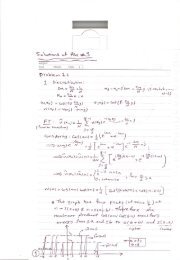
Solutions I

MAE294B/SIO203B: Methods in Applied Mechanics Winter Quarter 2011
http://maecourses.ucsd.edu/mae294b
Solutions I
1 The fixed points are solutions of 2/(x 2 + 1) − x 2 = 0, which gives the biquadratic x 4 + x 2 − 2 =
(x 2 + 2)(x 2 − 1) = 0. The imaginary roots are not relevant so the fixed points are at −1 and 1.
Calculate f ′ (x) = −4x(x 2 + 1) −1 − 2x, so that f ′ (−1) = −3 and f ′ (1) = 3. Hence −1 is unstable
and 1 is stable. The exact solution can be found by separating variables:
x2 + 1
(x2 + 1)(x2 dx = dt.
− 1)
This integrates to
t = 1
3 √
tan
2
−1 (x0/ √ 2) − tan −1 (x/ √
2) + 1
3 log (x + 1)(x0 − 1)
(x − 1)(x0 + 1) ,
where x(0) = x0. It is clear that t → ∞ corresponds to x → 1 while t → −∞ corresponds to x → −1.
2 Transforming to polar coordinates gives
Hence we need to solve the system
r˙r = x ˙x + y ˙y = r 2 − r 4 , r 2 ˙θ = x ˙y − y ˙x = r 2 .
˙r = r(1 − r 2 ),
˙θ = 1.
The equations decouple. The angle θ increases linearly with time: θ = θ0 + t. The modulus r
satisfies a nonlinear equation. A phase line analysis shows that 0 is unstable and 1 is stable. Hence
(0,0) is a fixed point, which must be an unstable anticlockwise focus from the form of the r- and
θ-equations, and any other initial condition tends to a periodic orbit with r = 1. The solution to the
r-equation has the solution r = [1 + (r −2
0 − 1)e−t/2 )] −1/2 .
3 (a) The fixed points are at (0,0), (1,0), (0,2) and ( 1 2 , 1 2 ). The matrix of derivatives is
1 − 2y1 − y2 −y1
D =
− 3 4y2 1
2 − 1 2y2 − 3 4y1
.
For the fixed point at (0,0),
1 0
D =
0 1 2
This is an unstable node. For the fixed point at (1,0),
−1 −1
D =
0 − 1
4
with eigenvalues/vectors 1, 1 2 and (1,0)T ,(0,1) T .
with eigenvalues/vectors −1,− 1 4 and (1,0)T ,(4,−3) T .
1

This is a stable node. For the fixed point at (0,2),
−1
D =
−
0
3 2 − 1 2
This is a stable node. For the fixed point at ( 1 2 , 1 2 ),
1 −
D = 2 − 1 2
− 3 8 − 1
8
with eigenvalues/vectors −1,− 1 2 and (1,3)T ,(0,1) T .
with eigenvalues − 5
16 ±
√
57
16 .
This is a saddle.
(b) The fixed point is at (0,0). The matrix of derivatives is
0 1
D =
∓2a2y1y2 − 1 ±a2 (1 − y2 1 )
=
0 1
−1 ±a 2
For |a| < √ 2, the fixed point is a clockwise focus, unstable for + and stable for −. For |a| > √ 2,
the fixed point is an unstable node for + and stable for −.
(c) There are fixed points at (0,0) and at (−1.19,−1.48). The second corresponds to y∗ 2 = − 1 6 (270+
6 √ 2019) 1/3 − (270 + 6 √ 2019) −1/3 and y∗ 1 = 2y∗2 /(1 − y∗2 ). The matrix of derivatives is
For the fixed point at (0,0),
2 1
D =
1 −2
D =
This is a saddle. For the other fixed point,
−1.24 −6.84
D =
2.48 −0.81
2 + y 3 2 1 + 3y1y 2 2
1 − y2 −2 − y1
.
.
with √ 5,− √ 5 and (1, √ 5 − 2) T ,(2 − √ 5,1) T .
with eigenvalues −1.02 ± 4.11i.
This is an anticlockwise stable focus.
(d) The question in the book has changed from edition to edition. In the old one, the set of equations
is
˙y1 = y2, ˙y2 = siny2 − y1.
The fixed point is (0,0). The matrix of derivatives is
0
D =
−1
1
cosy2
=
This is a clockwise unstable focus.
In the new one, the set of equations is
0 1
−1 1
˙y1 = y2, ˙y2 = siny1 − y2.
2
.

The fixed points are at (nπ,0). The matrix of derivatives is
0 1
D =
cosy1 −1
For even n, these are saddles with λ = − 1 2 ±
√ 3
2 .
λ = − 1 2 ± i
(e) The fixed point is (0,0). The matrix of derivatives is
2 − 6y2 D =
1 − 2y2 2 1 − 4y1y2
−1 0
√ 5
2 . For odd n, these are anticlockwise stable foci with
=
2 1
−1 0
This is a degenerate unstable node with eigenvalue/eigenvector 1 and (1,−1) T .
2.5
2
1.5
1
0.5
0
−0.5
3
2
1
0
−1
−2
−3
3
2
1
0
−1
−2
−3
3
2
1
0
−1
−2
−3
(a)
0 1 2
(b) −3
−2 0 2
(d) old
−2 0 2
(e)
−2 0 2
3
2
1
0
−1
−2
−3
0.5
0
−0.5
−1
−1.5
−2
−2.5
10
5
0
−5
(b) +1
−2 0 2
(c)
−2 −1 0
(d) new
.
−10
−10 0 10
0.5
Figure 1: Phase planes for 3.
3
0
(e)
−0.5
−0.5 0 0.5