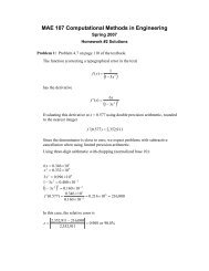
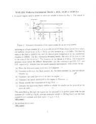
solution

ω = 100 . For low frequency ( ω ω 10 ), it’s a straight line with a slope of 0 at
p
p
phase equals 0. For high frequency ( ω 10ω p ), it’s a straight line with a slope of 0 at
phase equals − π . Then for frequencies between them ( ω 10 < ω < 10ω
), the
p p
straight line (reference to log10 ω ) achieves the − π phase change, as shown (dotted
line). Then, get the phase asymptote by applying composition rules: dashed line plus
dotted line, as shown (solid line).
phase factor
phase factor
Code:
2
0
-2
-4
10 0
2
1
0
-1
-2
10 0
10 1
10 1
clear all
omg = 1:1:10000;
asym_z = 20*log10(omg/500); % get the magnitude asymptote from zero
figure(2),subplot(2,1,1),semilogx(omg,asym_z,'--'),hold on
xlabel('\omega'),ylabel('gain factor')
asym_z_ph = pi/2*ones(size(omg)); % get the phase asymptote from zero
figure(3),subplot(2,1,1),semilogx(omg,asym_z_ph,'--'),hold on
xlabel('\omega'),ylabel('phase factor')
omg_p = 100;
omg1 = 1:1:omg_p;
10 2
ω
10 2
ω
10 3
10 3
10 4
10 4