solution

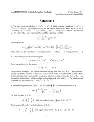
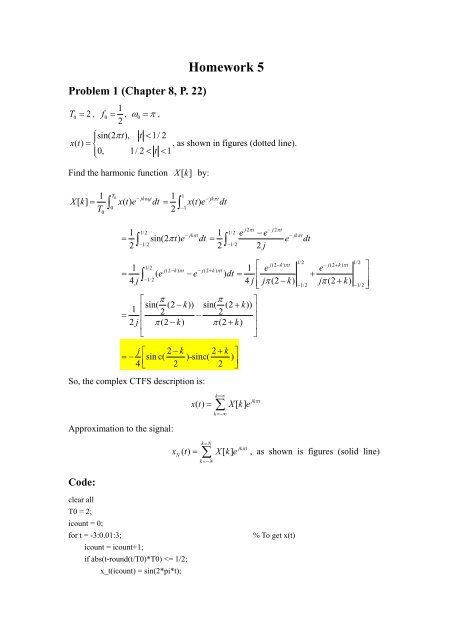
Problem 1 (Chapter 8, P. 22)
T 0 = 2 , 0
1
f = , ω0 = π ,
2
Homework 5
⎧ ⎪sin(2
πt),
t < 1/ 2
xt () = ⎨
, as shown in figures (dotted line).
⎪⎩ 0, 1/ 2 < t < 1
Find the harmonic function X[ k ] by:
1
T0
− jkω0t X[ k] = x( t) e dt
T ∫0
0
1
=
2 ∫
1/2
−1/2
1
=
2 ∫
1
−1
− jkπt x() te dt
− jkπt 1
sin(2 πte
) dt=
∫
e − e
j
j2πt − j2πt 1/2
− jkπ t
e dt
2 −1/2
2
(2 )
1/2
(2 )
1/2
1 1/2
j(2 −k) πt − j(2 + k) πt
1 ⎡ j −k πt − j + k πt
e e ⎤
= ( e −e
) dt
4 j ∫
= ⎢ +
⎥
−1/2
4 j ⎢ jπ(2 − k) jπ(2 + k)
⎣ −1/2 −1/2⎥⎦
⎡ π π ⎤
sin( (2 )) sin( (2 ))
1 ⎢
− k + k
2 2 ⎥
= ⎢ −
⎥
2 j
⎢ π(2 − k) π(2
+ k)
⎥
⎣ ⎦
j ⎡ 2− k 2+
k ⎤
=− sin c( )-sinc( )
4⎢ ⎣ 2 2 ⎥
⎦
So, the complex CTFS description is:
Approximation to the signal:
Code:
k =∞
jk t
x() t X[ k] e π
= ∑
k= N
k =−∞
jk t
xN () t X[ k] e π
= ∑ , as shown is figures (solid line)
k=−N clear all
T0 = 2;
icount = 0;
for t = -3:0.01:3; % To get x(t)
icount = icount+1;
if abs(t-round(t/T0)*T0)

else x_t(icount) = 0;
end
end
tt = -3:0.01:3;
figure(1);subplot(2,1,1),plot(tt,x_t,':');hold on
x_Nt = zeros(size(t)); % To get x[k]
N = 1; % N=1,2,3
for k = 1:N;
X_k1(k) = -j/4*(sinc((2-k)/2)-sinc((2+k)/2));
X_k2(k) = -j/4*(sinc((2+k)/2)-sinc((2-k)/2));
x_Nt = x_Nt+X_k1(k)*exp(j*2*pi*k*1/T0*tt)++X_k2(k)*exp(-j*2*pi*k*1/T0*tt);
end
figure(1);subplot(2,1,1),plot(tt,x_Nt);hold off
N=1
1
x(t)
x(t)
x(t)
0.5
0
-0.5
-1
-3 -2 -1 0 1 2 3
1
0.5
0
-0.5
-1
-3 -2 -1 0 1 2 3
1
0.5
0
-0.5
t
N=2
-1
-3 -2 -1 0 1 2 3
t
N=3
t

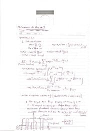
Problem 2 (Chapter 8, P. 23)
From (a) to (d), we got
x () t = x () t + 2cos(2 Nπt) N N−1
= x ( t) + 2cos(2( N − 1) πt) + 2cos(2 Nπt)
N −2
= x ( t) + 2cos(2 πt) + 2cos(4 πt) + + 2cos(2 Nπt)
0
N
= 1+∑ 2 cos(2 nπt) = ∑ e
n=
1
N
n=−N j2nπt Signals for N = 0,1,2,20 are shown as follow over the time range − 3< t < 3.
By
numerically calculate the area of the signal over − 1/2 < t < 1/2,
we got:
( a) N = 0, area=
1,
( b) N = 1, area=
1,
() c N = 2, area=
1,
( d) N = 20, area=
1
As N become lager, for case N = ∞ ,
j2nπt x () t = ∑ e tends to a function x() t
N
∞
n=−∞
with 0 1 T = and Xk [ ] = 1.
From the table we can find that, x() t is a unit period
impulse ( xt ( ) = δ ( t) ↔ Xk [ ] = 1).
Clearly see in plots, as N increases the figure
become more like the impulse train and the area within one period should be 1.
Code:
t = -3:0.01:3; x_Nt = zeros(size(t))+1; N0 = 20; % N0=0,1,2,20 for part a,b,c,d
for n = 1:N0;
x_Nt = x_Nt+2*cos(2*n*pi*t);
end
figure(2),subplot(2,1,1),plot(t,x_Nt);
num1 = find(t==-1/2);num2 = find(t==1/2);
Area = sum((x_Nt(num1:num2-1))*0.01, % Summation should end at num2-1
N=0
2
x 0 (t)
1.5
1
0.5
0
-3 -2 -1 0 1 2 3
t

x 1 (t)
x 2 (t)
x 20 (t)
3
2
1
0
N=1
-1
-3 -2 -1 0 1 2 3
6
4
2
0
-2
-3 -2 -1 0 1 2 3
60
40
20
0
t
N=2
-20
-3 -2 -1 0 1 2 3
Problem 3 (Chapter 8, P. 30)
t
N=20
(1) From the first figure in Figure E.30, the signal is even with T0 = 2, ω0 = π
So,
1
T0
− jkω0t X[ k] = x( t) e dt
T ∫0
0
1
=
2 ∫
1
−1
t
− jkπt x() te dt
1 1
= x( t)[cos( kπt) jsin( kπt)] dt
2 ∫ − + −
−1
1 1 j 1
= ()cos( ) ()sin( )
2∫ x t kπt dt− x t kπt dt
−1 2∫−1
even odd
j 1
()sin( ) 0
2 ∫ x t kπt dt = , the harmonic function X[ k ] have a purely real value
−1

for every value of k .
(2) From the second figure in Figure E.30, the signal is odd with T0 = 1, ω0 = 2π
1
T0
− jkω0t X[ k] = x( t) e dt
T ∫0
0
1/2
= ∫
1/2
2
1/2 ()
− jk πt
x te dt
−
1/2 1/2
∫ ∫
= x( t)cos(2 kπt) dt− j x( t)sin(2 kπt) dt
−1/2 −1/2
odd
even
So, x()cos(2 t k t) dt 0
1/2 π ∫ = , the harmonic function X[ k ] have a purely imaginary
−
value for every value of k .
Problem 4 (Chapter 8, P. 32)
Period of a sine wave is
1
6
10 ; period of a burst of “1” is 1
; period of a burst of “0”
5
10
1
is 5
10 ; period of a binary signal with alternating 1’s and 0’s is 1
T 0 = 2× and 5
10
ω π
5
0 = × 10 . The binary signal we want should be like:
x(t)
1
0.5
0
-0.5
-3 -2 -1 0 1 2 3
x 10 -5
-1
t
How can it come?
As we already know the basic sine wave is
x 1 (t)
1
0.5
0
-0.5
x t = × t , shown as
6
1 () sin(210 ) π
-3 -2 -1 0 1 2 3
x 10 -5
-1
t
In order to get the wanted signal, the signal shown above should multiply with a

square wave signal 2 () x t looks like:
x 2 (t)
1
0.5
0
-0.5
-3 -2 -1 0 1 2 3
x 10 -5
-1
t
How to get this square wave signal? It’s just from a similar and basic function 3 () x t ,
as shown below. Then x2() t = x3() t × 2− 1.
x 3 (t)
1
0.5
-3 -2 -1 0 1 2 3
x 10 -5
0
t
The expression for this x3 () t is just a convolution of a rectangle function and
impulse train:
⎛ t ⎞
x3() t = rect ⎜ δ 5 5 () t 21/10 × 1/10
⎟∗
⎝ ⎠
⎛ t ⎞
x () 2 x () t − 1= 2rect ∗ () t − 1
⎝1/10 ⎠
⇒ 2 t = 3 ⎜ δ 5 ⎟
5 21/10 ×
6 ⎛ ⎛ t ⎞
⎞
xt () = x1() t x2() t = sin(2× 10 πt) ×⎜2rect ⎜ 5 δ 5 () t 1
21/10 × ⎟
1/10
⎟∗
−
⎝ ⎝ ⎠
⎠
1
From Fourier Series Pairs table, with T 0 = 2× 5
10
,
1
rectangular function is T = 5
10
,
ω π
5
0 = × 10 , width of

5 5 5
⎡ ⎛ × kπ
× ⎞ ⎤
⎢ 5 ⎜ ⎟ ⎥
1 1/10 1/10 10
X[ k] = ⎡δ[ k 20 ] δ[ k 20] 2 sinc
δ[
k]
2j ⎣ − − + ⎤⎦∗
× −
⎣ 2/10 ⎝ 2 ⎠ ⎦
1
⎡ ⎛kπ⎞ ⎤
= ⎡δ[ k 20 ] δ[ k 20] ⎤ sinc δ[
k]
2j ⎣ − − + ⎦∗⎢⎜
⎟−
2
⎥
⎣ ⎝ ⎠ ⎦
j ⎡ ⎛( k− 20) π ⎞ ⎛( k+
20) π ⎞
⎤
=− sinc sinc δ[ k 20 ] δ[
k 20]
2
⎢ ⎜ ⎟−⎜ ⎟−−
+ +
2 2
⎥
⎣ ⎝ ⎠ ⎝ ⎠
⎦
The magnitude and phase of the harmonic function are shown as follow:
|X[k]|
Phase of X[k]
Code:
0.1
0.05
0
-30 -20 -10 0 10 20 30
2
1
0
-1
-2
-30 -20 -10 0 10 20 30
k = -30:30;
N_k = 1/(2*j).*(sinc(pi/2.*(k-20))-sinc(pi/2.*(k+20))-dirac(k-20)+dirac(k+20));
figure(1), subplot(2,1,1),stem(k,abs(N_k),'fill'),
figure(1), subplot(2,1,2),stem(k,angle(N_k),'fill'),
Problem 5 (Chapter 12, P. 32)
10 jω10 jω
jω+ 10 jω+ 10 ( jω) + 20 jω+
100
(b). H( jω)
= ⋅ = 2
Code:
k
k

omg = 0.1:0.1:1000;
num = [10,0];den = [1,20,100];
sys = tf(num,den);
figure(1),bode(omg,sys);grid on; % using "bode" to get the Bode diagram
Magnitude (dB)
Phase (deg)
0
-20
-40
-60
90
45
0
-45
-90
10 -1
Asymptote:
10 0
j10ω
H( jω)
=
( jω
+ 10)
2
10 1
10 2
10 jω
= ⋅
jω+ 10 jω+
10
From the expression, we see the frequency response have: zero at jω = 0 , pole at
jω =− 10 and pole at jω =− 10 .
(1). Magnitude asymptote
First consider the part
10
jω + 10
10
20log10 0
10 = . For high frequencies ( ω ω p
10 3
. For low frequencies ( ω ω p ), the dB-scale magnitude is
20log
), magnitude should be 10
10
, which
jω
is a straight line with the slope of -20dB and go through (10,0). The magnitude
asymptote from
10
jω + 10
is a pair of straight lines with corner frequency at ω p = 10 ,

as shown (dashed line).
Similarly, for part
jω
jω
+ 10
jω jω
20log ≈ 20log
jω
+ 10 10
, 10 10
at low frequencies
( ω ω p ), which is a straight line with the slope of 20dB and go through (10,0). At high
frequencies ( ω ω p
asymptote from
(dotted line).
jω jω
20log ≈ 20log = 0 . So, the magnitude
jω+ 10 jω
), 10 10
jω
jω
+ 10
is also a pair of straight lines intersect at ω = ω p , as shown
At last, applying compose the dashed line and dotted line to get the final magnitude
asymptote, as shown (solid line).
gain factor
gain factor
0
-10
-20
-30
-40
10 -1
0
-10
-20
-30
-40
10 -1
(2). Phase asymptote
The phase asymptote from
( ω ω 10 ) and
p
10 0
10 0
10
jω + 10
10 1
ω
10 1
ω
10 2
10 2
10 3
10 3
contains three segments: 0 for low frequencies
π
− for high frequencies ( ω 10ω p ), and at frequencies around
2

π
ω p = 10 , a straight line (reference to log10 ω ) achieves the − phase change, as
2
shown (dashed line).
jω
π
Similarly, for part , for low frequencies ( ω ω p 10 ) and 0 for high
jω
+ 10 2
π
frequencies ( ω 10ω p ), a straight line at ω p /10 < ω < 10ωp
gives the − phase
2
change, as shown (dotted line).
At last, applying composition rules to get the final phase asymptote, as shown (solid
line).
phase factor
phase factor
Code:
2
1
0
-1
-2
10 -1
2
1
0
-1
-2
10 -1
10 0
10 0
omg = 0.1:0.1:1000;
omg_p = 10;
omg1 = 0.1:0.1:omg_p;
omg2 = omg_p+0.1:0.1:1000;
ym = zeros(size(omg));
ym_1 = ones(size(omg1)); % get the magnitude asymptote for low frequency
ym_2 = omg_p./omg2; % get the magnitude asymptote for high frequency
ym(1:length(omg1)) = ym_1;
ym(length(omg1)+1:end)= ym_2;
10 1
ω
10 1
ω
10 2
10 2
10 3
10 3

asym_1 = 20*log10(ym);
figure(2),subplot(2,1,1),semilogx(omg,asym_1,'--'),hold on
xlabel('\omega'),ylabel('gain factor')
zm = zeros(size(omg));
zm_1 = omg1/omg_p; % get the magnitude asymptote from the pole for low frequency
zm_2 = ones(size(omg2)); % get the magnitude asymptote from the pole for high frequency
zm(1:length(omg1)) = zm_1;
zm(length(omg1)+1:end) = zm_2;
asym_2 = 20*log10(zm);
figure(2),subplot(2,1,1),semilogx(omg,asym_2,':'),hold off
omg3 = 0.1:0.1:omg_p/10;
omg4 = omg_p/10+0.1:0.1:omg_p*10;
omg5 = omg_p*10+0.1:0.1:1000;
yp = zeros(size(omg));
yp_1 = zeros(size(omg3)); % phase is zero for low frequency
yp_2 = -1*pi/2/2*(log10(omg4)-log10(omg_p/10));
% a -pi/2 phase change from omg_p/10 to omg_p*10
yp_3 = -1*pi/2*ones(size(omg5)); % phase is -pi/2 for high frequency
yp(1:length(omg3)) = yp_1;
yp(length(omg3)+1:length(omg3)+length(omg4))= yp_2;
yp(length(omg3)+length(omg4)+1:end)= yp_3;
asym_1_ph = yp;
figure(3),subplot(2,1,1),semilogx(omg,asym_1_ph,'--'),hold on
xlabel('\omega'),ylabel('phase factor')
zp = zeros(size(omg));
zp_1 = pi/2*ones(size(omg3)); % phase is pi/2 for low frequency
zp_2 = -1*pi/2/2*(log10(omg4)-log10(omg_p*10));
% a -pi/2 phase change from omg_p/10 to omg_p*10
zp_3 = zeros(size(omg5)); % phase is 0 for high frequency
zp(1:length(omg3)) = zp_1;
zp(length(omg3)+1:length(omg3)+length(omg4))= zp_2;
zp(length(omg3)+length(omg4)+1:end)= zp_3;
asym_2_ph = zp;
figure(3),subplot(2,1,1),semilogx(omg,asym_2_ph,':'),hold off
asym_m = asym_1+asym_2; % composition for magnitide
figure(2),subplot(2,1,2),semilogx(omg,asym_m),
xlabel('\omega'),ylabel('gain factor')
asym_ph = asym_1_ph+asym_2_ph; % composition for phase
figure(3),subplot(2,1,2),semilogx(omg,asym_ph),
xlabel('\omega'),ylabel('phase factor')
j20ω 20 jω
( )
10000 − ω + j20 ω ( jω) + 20 jω+
10000
(c). H jω=
=
2 2

Code:
omg = 0.01:0.01:10000;
num = [20,0];den = [1,20,10000];
sys = tf(num,den);
figure(1),bode(omg,sys);grid on
Magnitude (dB)
Phase (deg)
0
-10
-20
-30
-40
90
45
0
-45
-90
10 1
Asymptote:
Bode Diagram
10 2
Frequency (rad/sec)
j20ω
H( jω)
=
( jω+ 10 − j99.5)( jω+ 10 + j99.5)
ω
j
j20ω
=
= 500
2
2
⎡ ω ω ⎤
10000 ⎢1− + j
⎛ ω ⎞ ω
10000 500
⎥ 1−
⎜ ⎟ + j
⎣ ⎦ ⎝100 ⎠ 500
From the expression, we see the frequency response have: zero at jω = 0 , a pair of
complex conjugate poles at jω =− 10 + j99.5
and jω = −10 − j99.5
.
(1). Magnitude asymptote
10 3

The dB-scale magnitude asymptote from zero j
500
ω is a straight line with a slope of
20dB and go through (500,0), as shown (dashed line).
The dB-scale magnitude asymptote from pole
⎛ ω ⎞ ω
1−
⎜ ⎟ + j
⎝100 ⎠ 500
2
is a pair of straight
lines and ω p = 100 . For low frequency ( ω ω p ), it’s a straight line with a slope of
0dB. For high frequency ( ω ω p ), it’s a straight line with a slope of -40dB. These
two asymptotes intersect at ω = ω p , as shown (dotted line).
Then, applying composition rules to get the final magnitude asymptote: dashed line
plus dotted line, as shown (solid line).
gain factor
gain factor
50
0
-50
-100
-10
-20
-30
-40
-50
-60
10 0
10 0
(2). Phase asymptote
10 1
10 1
10 2
ω
10 2
The phase asymptote from zero j
500
ω is a straight line with a slope of 0 at phase
π
equals , as shown (dashed line).
2
The phase asymptote from pole
ω
⎛ ω ⎞ ω
1−
⎜ ⎟ + j
⎝100 ⎠ 500
2
10 3
10 3
10 4
10 4
contains three segments and

ω = 100 . For low frequency ( ω ω 10 ), it’s a straight line with a slope of 0 at
p
p
phase equals 0. For high frequency ( ω 10ω p ), it’s a straight line with a slope of 0 at
phase equals − π . Then for frequencies between them ( ω 10 < ω < 10ω
), the
p p
straight line (reference to log10 ω ) achieves the − π phase change, as shown (dotted
line). Then, get the phase asymptote by applying composition rules: dashed line plus
dotted line, as shown (solid line).
phase factor
phase factor
Code:
2
0
-2
-4
10 0
2
1
0
-1
-2
10 0
10 1
10 1
clear all
omg = 1:1:10000;
asym_z = 20*log10(omg/500); % get the magnitude asymptote from zero
figure(2),subplot(2,1,1),semilogx(omg,asym_z,'--'),hold on
xlabel('\omega'),ylabel('gain factor')
asym_z_ph = pi/2*ones(size(omg)); % get the phase asymptote from zero
figure(3),subplot(2,1,1),semilogx(omg,asym_z_ph,'--'),hold on
xlabel('\omega'),ylabel('phase factor')
omg_p = 100;
omg1 = 1:1:omg_p;
10 2
ω
10 2
ω
10 3
10 3
10 4
10 4

omg2 = omg_p+1:1:10000;
ym = zeros(size(omg)); % get the magnitude asymptote from the pole for low frequency
ym_1 = ones(size(omg1)); % get the magnitude asymptote from the pole for high frequency
ym_2 = omg2/omg_p;
ym(1:length(omg1)) = ym_1;
ym(length(omg1)+1:end)= ym_2;
asym_p = -40*log10(ym);
figure(2),subplot(2,1,1),semilogx(omg,asym_p,':'),hold off
omg3 = 1:1:omg_p/10;
omg4 = omg_p/10+1:1:omg_p*10;
omg5 = omg_p*10+1:1:10000;
yp = zeros(size(omg));
yp_1 = zeros(size(omg3));
yp_2 = -1*pi/2*(log10(omg4)-log10(omg_p/10));
% a -pi/2 phase change from omg_p/10 to omg_p*10
yp_3 = -1*pi*ones(size(omg5));
yp(1:length(omg3)) = yp_1;
yp(length(omg3)+1:length(omg3)+length(omg4))= yp_2;
yp(length(omg3)+length(omg4)+1:end)= yp_3;
asym_p_ph = yp;
figure(3),subplot(2,1,1),semilogx(omg,asym_p_ph,':'),hold off
asym_m = asym_z+asym_p; % composition for magnitude asymptote
figure(2),subplot(2,1,2),semilogx(omg,asym_m),
xlabel('\omega'),ylabel('gain factor')
asym_ph = asym_z_ph+asym_p_ph;
figure(3),subplot(2,1,2),semilogx(omg,asym_ph), % composition for phase asymptote
xlabel('\omega'),ylabel('phase factor')