Norm 3

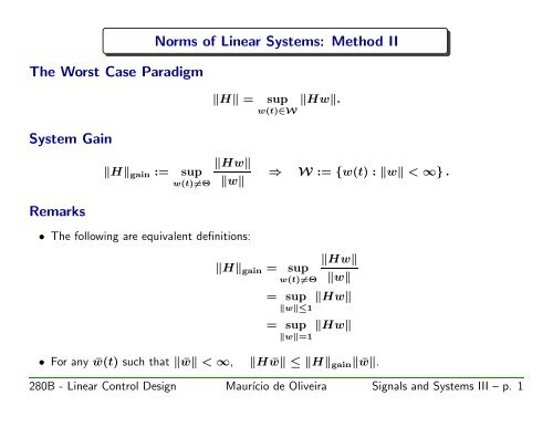
The Worst Case Paradigm
System Gain
Remarks
Norms of Linear Systems: Method II
Hgain := sup
w(t)=Θ
H = sup
w(t)∈W
Hw.
Hw
w
• The following are equivalent definitions:
Hgain = sup
w(t)=Θ
⇒ W := {w(t) : w < ∞} .
Hw
w
= sup Hw
w≤1
= sup Hw
w=1
• For any ¯w(t) such that ¯w < ∞, H ¯w ≤ Hgain ¯w.
280B - Linear Control Design Maurício de Oliveira Signals and Systems III – p. 1

Definition (SISO system)
Definition (MIMO system)
L2 − L2 Gain
H∞ := sup
ω
H∞ Norm
H∞ := sup
ω
|H(jω)|.
H(jω), H(jω) 2 = λmaxH(jω) ∗ H(jω).
HL2−L2 := sup
w(t)=Θ
Hw2
.
w2
Proposition For an asymptotically stable linear system HL2−L2 = H∞.
280B - Linear Control Design Maurício de Oliveira Signals and Systems III – p. 2

On the Frequency Domain:
Compute
On the Time Domain:
Compute
Computing the H∞ Norm
H 2
∞
= sup
ω
H(jω).
H∞ = Hwwc2, wwc := arg sup
w2=1
Hw2.
280B - Linear Control Design Maurício de Oliveira Signals and Systems III – p. 3

Bounded Real Lemma
Computing the H∞ Norm
Consider the asymptotically stable CTLTI system with minimal realization
H(s) = C (sI − A) −1 B + D and null initial conditions. There exists P ∈ Sn such that
⎡
⎤
if, and only if, H∞ < µ.
P ≻ Θ,
⎢
⎣
A T P + P A P B C T
⎥
⎦ ≺ Θ
C D −µI
B T P −µI D T
280B - Linear Control Design Maurício de Oliveira Signals and Systems III – p. 4

Computing the H∞ Norm
Proof (Sufficiency) Define the quadratic Lyapunov function V (x) := xT P x, P ∈ Sn and
its time-derivative
˙V (x) = 2x T P Ax + x T ⎛
P Bw = ⎝ x
⎞T
⎡
⎠ ⎣
w
AT P + P A P B
BT ⎤ ⎛
⎦ ⎝
P Θ
x
⎞
⎠ .
w
Assume that the BRL holds and apply Schur complement to obtain
⎡
⎣ AT P + P A + µ −1 C T C P B + µ −1 C T D
B T P + µ −1 D T C −µI + µ −1 D T D
⎤
⎦ ≺ Θ.
280B - Linear Control Design Maurício de Oliveira Signals and Systems III – p. 5

Notice that for all w(t) ∈ L2
⎡
⎡
Computing the H∞ Norm
⎣ AT P + P A + µ −1C T C P B + µ −1C T D
BT P + µ −1DT C −µI + µ −1DT D
⎣ AT P + P A P B
B T P Θ
⎤
⎦ ≺ µ
⎛
⎝
⇓
x
⎞T
⎡
⎠ ⎣
w
AT P + P A
B
P B
T P
⎤ ⎛
⎦ ⎝
Θ
x
⎞ ⎛
⎠ < µ ⎝
w
˙V (x)
x
⎞
⎠
w
⎡
⇕
⎤
⎦ ≺ Θ,
⎣ −µ−2C T C −µ −2C T D
−µ −2DT C I − µ −2DT D
T ⎡
⎤
⎦ ,
⎣ −µ−2C T C −µ −2C T D
−µ −2DT C I − µ −2DT D
⎤ ⎛
⎦ ⎝ x
⎞
⎠ .
w
w T w−µ −2 z T z
280B - Linear Control Design Maurício de Oliveira Signals and Systems III – p. 6

Integrating
on both sides
Computing the H∞ Norm
∞
0
˙V (x) < µ w T w − µ −2 z T z
˙V (x) dt < µ
V (x(∞)) − V (x(Θ)) < µ
∞
0
∞
0
w T w − µ −2 z T z dt,
w T w − µ −2 z T z dt.
280B - Linear Control Design Maurício de Oliveira Signals and Systems III – p. 7

Computing the H∞ Norm
Since the system is asymptotically stable, the output z(t) ∈ L2 for all w(t) ∈ L2. Using the
minimality of the realization
z(t) ∈ L2 ⇔ x(t) ∈ L2 ⇒ x(∞) = Θ ⇒ V (x(∞)) = 0.
From the null initial conditions V (0) = 0. Hence
∞
0
Consequently
w T w − µ −2 z T z dt > 0 ⇒
∞
w
0
T w dt > µ −2
∞
0
z2 < µw2, ∀w(t) ∈ L2 ⇒ µ > H∞
since z2 = Hw2 ≤ H∞w2 for all w(t) ∈ L2.
z T z dt.
280B - Linear Control Design Maurício de Oliveira Signals and Systems III – p. 8

Theorem
Small Gain Theorem
PSfrag replacements
If G∞ < 1 the unity feedback connection is asymptotically stable.
e w z
That is, z(t), w(t) ∈ L2 for all e(t) ∈ L2.
H(s) G(s)
Proof
Hence
z = Gw = G(z + e), ⇒ z2 ≤ G∞z + e2 ≤ G∞(z2 + e2)
(1 − G∞)z2 ≤ G∞e2 ⇒ z2 ≤
Finally, e(t), z(t) ∈ L2 ⇒ w(t) ∈ L2.
G∞
(1 − G∞) e2 < ∞ ⇒ z(t) ∈ L2
280B - Linear Control Design Maurício de Oliveira Signals and Systems III – p. 9

Theorem
Small Gain Theorem
PSfrag replacements
If G∞ < µ and H∞ < µ −1 the feedback
connection is asymptotically stable. That is,
z1(t), w1(t), z2(t), w2(t) ∈ L2 for all e1(t), e2(t) ∈ L2.
Remark If H(s) = ∆ then Small Gain ⇒ Robust Stability.
z2 H(s)
w2
e1 w1 z1
G(s)
280B - Linear Control Design Maurício de Oliveira Signals and Systems III – p. 10
e2

Proof
acements
Introduce scalings
PSfrag replacements
e1
and work with the modified connection
µe1
z2
w1
µ
G(s)
H(s)
Small Gain Theorem
H(s)
µ µ −1
PSfrag
G(s)
replacements
µ −1
w2
z1
e2
⇔
e2
z2 µH(s)
w2
µe1 w1 z1
µ −1 G(s)
280B - Linear Control Design Maurício de Oliveira Signals and Systems III – p. 11
e2

⎛
⎝ z1
z2
Small Gain Theorem
⎞ ⎡
⎠ = ⎣ µ−1 ⎤ ⎛
G Θ
⎦ ⎝
Θ µH
w1
⎞ ⎡
⎠ = ⎣
w2
µ−1 ⎤ ⎛⎛
G Θ
⎦ ⎝⎝
Θ µH
µe1
⎞ ⎛
⎠ + ⎝
e2
z2
⎞⎞
⎠⎠
,
z1
⎡
z1
⇒
≤ ⎣
z2
2
µ−1 ⎤
⎛
⎞
G Θ µe1
z2
⎦
⎝
+ ⎠
,
Θ µH e2 z1
∞
2
2
z1
⇒
≤ max{µ
z2
2
−1 ⎛
⎞
µe1
z1
G∞, µH∞} ⎝
+ ⎠
,
e2 z2
2
2
z1
⇒
≤
max{µ−1G∞, µH∞}
1 − max{µ −1
µe1
G∞, µH∞}
< ∞,
z2
2
⇒ z1(t), z2(t) ∈ L2.
Finally, e1(t), e2(t), z1(t), z2(t) ∈ L2 ⇒ w1(t), w2(t) ∈ L2.
280B - Linear Control Design Maurício de Oliveira Signals and Systems III – p. 12
e2
2

Hp Spaces
The set of (rational) matrix functionals H(s) : C → C m×n analytic in the open left semiplane
of the complex plane and equipped with the norm Hp, p = 2, ∞, is a normed vector space.
This space is denoted by the symbol Hp (RHp). If Hp < ∞ then H(s) ∈ Hp (RHp).
Remarks
• Analytic in the left part of the complex plane ⇒ continuous-time stability.
• If H(s) ∈ RHp, analytic in the left part of the complex plane ⇒ no “unstable”
continuous-time poles.
• H(s) ∈ RH2 ⇒ H(s) is asymptotically stable and strictly proper.
• H(s) ∈ RH∞ ⇒ H(s) is asymptotically stable.
280B - Linear Control Design Maurício de Oliveira Signals and Systems III – p. 13

Hp Spaces
The set of (rational) matrix functionals H(z) : C → C m×n analytic in the open unity circle and
equipped with the norm Hp, p = 2, ∞, is a normed vector space. This space is denoted by
the symbol Hp (RHp). If Hp < ∞ then H(z) ∈ Hp (RHp).
Remarks
• Analytic in the ⇒ discrete-time stability.
• If H(s) ∈ RHp, analytic in the plane ⇒ no “unstable” discrete-time poles.
• H(z) ∈ RH2 ⇒ H(z) is asymptotically stable.
• H(z) ∈ RH∞ ⇒ H(z) is asymptotically stable.
280B - Linear Control Design Maurício de Oliveira Signals and Systems III – p. 14