Frequency Response and Continuous-time Fourier Transform

Frequency Response and
Continuous-time Fourier Transform

Goals
Signals and Systems in the FD-part II
I. (Finite-energy) signals in the Frequency Domain
- The Fourier Transform of a signal
- Classification of signals according to their spectrum
(low-pass, high-pass, band-pass signals)
- Fourier Transform properties
II. LTI systems in the Frequency Domain
- Impulse Response and Frequency Response relation
- Computation of general system responses in the FD
III. Applications to audio signals
- A simple design of an equalizer

Objectives
How can we extend the Fourier Series method to other signals?
There are two main approaches:
The Fourier Transform (used in signal processing)
The Laplace Transform (used in linear control systems)
The Fourier Transform is a particular case of the Laplace
Transform, so the properties of Laplace transforms are
inherited by Fourier transforms. One can compute Fourier
transforms in the same way as Laplace transforms.

!
!
Fourier Transform
Generalization of Fourier Series to aperiodic functions
Recall, for a periodic function of period ,
$
%
x(t) = X[k]e jk" 0t
k =#$
For an aperiodic function, take
x(t) = 1
2" X( j#)e j#t %
& ! d#
1 4 4 4 4 $% 2 4 4 4 4 3
!
Requires x(t) to be absolutely integrable
!
!
x(t)
X[k] = 1
T0 !
T0 "#
$
%
T 0
2
$
" T0
2
T 0
x(t)e " jk# 0 t dt
X( j") = x(t)e # j"t dt
1 4 4 4 #$ 2 4 4 4 3
Inverse Fourier transform Fourier transform
# !
$ x(t) dt < #
"#
'
)
(
lim
1
T0 " # T0 $ d% *
,
2& +

General signals in the Frequency Domain
The signal representation in the Frequency Domain is the
graph of and of
One can classify signals into:
!
| F( j") |
!
"F( j#) = arctan(Im(F( j#) /Re(F( j#))
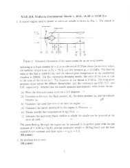
Low-pass signal: The energy of the signal is concentrated
at low frequencies (these signals have “slow transitions”
in the time domain and are smooth)
High-pass signal: The energy of the signal is concentrated
at high frequencies (these signals have zero mean and
rapidly changing values; e.g. noise)
Band-pass signal: The spectrum vanishes at low and high
frequencies and concentrates in an intermediate
frequency band (signals that look more like a pure
sinusoid with high frequency)

Graphical Interpretation TD versus FD
Examples using cyclic frequency:
Low-pass
Band-pass
High-pass

!
!
Examples: computation of FT
Let’s compute the FT of
$
Let’s compute the FT of
$
x(t)= e "a|t| , Re(a) > 0
X( j") = x(t)e
!
# j"t % dt = e
#$
#a|t| e # j"t % dt = e
#$
at # j"t % dt + e
#$
#at # j"t % dt
0
0
$
& 1 ) &
# j" )t 1 )
+ j" )t
= ( e(a + # ( e#(a +
' a # j" * a + j" #$ '
* 0
1
=
a # j" +
1
a + j" =
2a
a 2 +" 2
$
$
x(t)=1
X( j") = x(t)e
!
# j"t % dt = e
#$
# j"t % dt = ? Integral does not converge
#$
0
$

!
Computation of FT
What do we do? Calculate FT of and then take
Now,
Therefore,
X " ( j#) =
2"
" 2 +# 2
!
lim
" # 0 X " ( j$) = 0, if $ % 0
Similarly, one can also compute
!
!
X( j") = 2#$(")
!
x(t)e "#t , # > 0
lim
" # 0 X " ( j$) = %, if $ = 0
!
cos(at) " #($(% & a) +$(% + a))
sin(at) " j#($(% + a) &$(% & a))
!
&
'
%&
" #0
X " ( j#)d# = 2$

Graphical representation
Observe this is the same as the Fourier Series spectrum graphs!

TD and FD representation of a signal
The Time Domain and Frequency Domain representations are
used to emphasize different aspects
TD graph: you can see when something occurs and the
amplitude of occurrence. For example, this is good for
describing step or discontinuous signals
FD graph: the magnitude and phase gives you information
about what produces the oscillations present in the signal.
Good for describing audio signals
Example: sound from ringing a wine glass.
The harmonics, fundamental frequency, tells
us the nature of the material that produced
it. This information is not contained in a
single sample time of a TD description

TD versus FD: what to choose?
In general, the use of TD or FD signal representations depends
on the application you are working with
For ECG monitors, you want to emphasize time occurrences,
and produce filters that generate good step responses*. So
you study time domain representations of step responses
For a hearing aid, you want to emphasize certain frequency
ranges, so you want to optimize your filter with respect to
frequency responses. So you study frequency domain
representations of audio signals
Filters that perform well in terms of frequencies do not perform
well in terms of step responses, and the other way around
*a good step response should have a shape as close to a step as possible

Fourier Transform pairs Table
A few more examples of Fourier Transform pairs from the book
(Table 10.1, observe there are two columns, one for fand
one for )
!
!
!
!
!
"
!
!
1" 2#$(%)
u(t) " #$(%) + 1
j%
e "at u(t) # 1
j$ + a
cos(at) " #($(% & a) + $(% + a))
sin(at) " j#($(% + a) &$(% & a))
rect(t) " sinc(# /2$)
sinc(t) " rect(# /2$)
!

Fourier Transform properties (radian freq)
Linearity
Shift in time
Time scaling
Frequency scaling
Frequency shifting
Modulation
Differentiation
Integration
!
!
!
!
!
!
!
ax(t) + by(t) " aX( j#) + bY( j#)
" j$c
x(t " c) # X( j$)e
x(at) " 1 #
X( j
| a | a )
x(t)e j" 1 t
x( ) " X(aj#)
| a | a
0t
# X( j(" $"0))
x(t)sin" 0t # j
2 X( j" + j" [ 0) $ X( j" $ j" 0) ]
x(t)cos" 0t # 1
2 X( j" + j" [ 0) + X( j" $ j" 0) ]
t
%
#$
d n x(t)
dt n
" ( j# ) n
X( j#)
x ( " )d" & 1
X( j') + (X(0 )( j')
j'

Convolution property of Fourier transforms
Convolution/Multiplication duality:
h(t) " f (t) = h(t #$) f ($)d$ ' H( j()F( j()
#%
!
In particular we have
!
%
&
!
h(t) f (t) " 1
2# H( j$) * F( j$)
F
h(t) " $ # H( j%)

!
!
!
What are the implications?
For a stable linear system we can compute system responses as
( )
Y j" , X j" are signal Fourier transforms
H( j" )
is the system frequency response
Spectra
!
!
The Frequency Response contains all the information needed to
determine any system response
!
Deconvolutions can be computed by division in the FD:
y(t) = h(t) * x(t)
If , then
Y( j" ) = H( j" )X j"
(can be done for invertible systems)
!
( )
( )
Y( j") = H( j") X( j"), #Y( j") = #H( j") + #X( j")
x(t) = F "1 {Y( j#) /H( j#)}

Signals/systems in the FD
Similarly to the Fourier Series case, once the input signal and
system Fourier transforms are computed, the response
can be obtained through simple multiplication and sum
operations
Additionally, the FT/IFT can be approximated in a computer
through special routines: the FFT (Fast Fourier Transform)
and the IFFT (Inverse Fast Fourier Transform)
Overall, this makes the whole process in the FD much
faster than convolution in the TD. The only disadvantage
is that the FT only applies to finite energy signals

Goals
Signals/systems in the FD
I. (Finite-energy) signals in the Frequency Domain
- The Fourier Transform of a signal
- Classification of signals according to their spectrum (lowpass
signals, high-pass signals, band-pass signals)
- Fourier Transform properties
II. LTI systems in the Frequency Domain
- Impulse Response and Frequency Response relation
- Computation of general system responses in the FD
III. Applications to audio signals
- A simple design of an equalizer

A simple design of an equalizer
Applications of the Fourier Transform theory are many. One of
them is the design of equalizers to accomplish different
effects on audio signals:
-Bass volume or low frequencies in your audio system can
be implemented using a low-pass filter;
-Treble volume or high frequencies can be implemented
using a high-pass filter
!
H 1(") = " c
j" + " c
-The previous two filters can be combined together to
filter only those sounds with frequencies around a value of
!
!
H 2(") =
H 3 (") = " c
j" + " c
j"
j" + " c
#
j"
j" + " c
!
" c

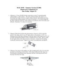
A simple design of an equalizer
Example graphs of these filters for a given values of
the cutoff frequencies " c#lowpass = 50000, " c#highpass =100
:
!
!

A simple design of an equalizer
Another example of band-pass filter centered at a
given frequency " 0 =1 and whose magnitude can
be adjusted is the following:
!
(Each color
corresponds to a different
choice of "
)
!
!
H1(") = ( j")2 + j2" 0" /10 # 2
+ " 0
( j") 2 + j2" 0" $10 # 2
+ " 0

A simple design of an equalizer
A simple equalizer can be built by “connecting in series” bandpass
filters like the previous one as follows:
The center frequencies of each band-pass filter are 20Hz, 30Hz,
40Hz,…. The Frequency Response of the equalizer is obtained
by summing all the band-pass filters’ FR. By choosing
different values of the parameters beta, one can emphasize
or de-emphasize any frequency range in an audio signal

Important points to remember:
Summary
A signal can be classified into a low-pass, high-pass or band-pass signal
depending on its magnitude and phase spectrum
In the time domain, low-pass signals correspond to signals with slow
transitions. High-pass signals correspond to signals with fast
transitions. Band-pass signals look like sinusoids/co-sinusoids.
The Fourier Transform theory allows us to extend the techniques and
advantages of Fourier Series to more general signals and systems
In particular we can compute the response of a system to a signal by
multiplying the system Frequency Response and the signal Fourier
Transform. (And we can avoid convolution)
The Fourier Transform of the Impulse Response of a system is precisely
the Frequency Response
The Fourier Transform theory can be used to accomplish different audio
effects, e.g. the design of equalizers