3+1 formalism and bases of numerical relativity - LUTh ...

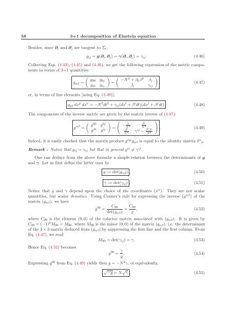
58 3+1 decomposition of Einstein equation
Besides, since ∂i and ∂j are tangent to Σt,
gij = g(∂i,∂j) = γ(∂i,∂j) = γij. (4.46)
Collecting Eqs. (4.43), (4.45) and (4.46), we get the following expression of the metric components
in terms of 3+1 quantities:
gαβ =
g00 g0j
gi0 gij
or, in terms of line elements [using Eq. (4.40)],
−N2 + βkβ
=
k βj
βi
γij
, (4.47)
gµν dx µ dx ν = −N 2 dt 2 + γij(dx i + β i dt)(dx j + β j dt) . (4.48)
The components of the inverse metric are given by the matrix inverse of (4.47):
g αβ
g00 g
=
0j
=
g i0 g ij
− 1
N2 βi N2 βj N2 γij − βiβj N2
. (4.49)
Indeed, it is easily checked that the matrix product g αµ gµβ is equal to the identity matrix δ α β .
Remark : Notice that gij = γij but that in general g ij = γ ij .
One can deduce from the above formulæ a simple relation between the determinants of g
and γ. Let us first define the latter ones by
g := det(gαβ) , (4.50)
γ := det(γij) . (4.51)
Notice that g and γ depend upon the choice of the coordinates (x α ). They are not scalar
quantities, but scalar densities. Using Cramer’s rule for expressing the inverse (g αβ ) of the
matrix (gαβ), we have
g 00 = C00
det(gαβ)
C00
= , (4.52)
g
where C00 is the element (0,0) of the cofactor matrix associated with (gαβ). It is given by
C00 = (−1) 0 M00 = M00, where M00 is the minor (0,0) of the matrix (gαβ), i.e. the determinant
of the 3 × 3 matrix deduced from (gαβ) by suppressing the first line and the first column. From
Eq. (4.47), we read
M00 = det(γij) = γ. (4.53)
Hence Eq. (4.52) becomes
g 00 = γ
. (4.54)
g
Expressing g 00 from Eq. (4.49) yields then g = −N 2 γ, or equivalently,
√ −g = N √ γ . (4.55)