3+1 formalism and bases of numerical relativity - LUTh ...

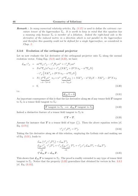
46 Geometry of foliations
Remark : In many numerical relativity articles, Eq. (3.27) is used to define the extrinsic curvature
tensor of the hypersurface Σt. It is worth to keep in mind that this equation has
a meaning only because Σt is member of a foliation. Indeed the right-hand side is the
derivative of the induced metric in a direction which is not parallel to the hypersurface
and therefore this quantity could not be defined for a single hypersurface, as considered in
Chap. 2.
3.3.6 Evolution of the orthogonal projector
Let us now evaluate the Lie derivative of the orthogonal projector onto Σt along the normal
evolution vector. Using Eqs. (A.8) and (3.22), we have
i.e.
Lmγ α β = mµ ∇µγ α β − γµ
β∇µm α + γ α µ
= Nn µ ∇µ(n α nβ) + γ µ
β
−γ α µ
= N( n µ ∇µn α
=N −1 D α N
µ
∇βm
α
NK µ + D α N nµ − n α ∇µN
NK µ
β + Dµ N nβ − n µ
∇βN
nβ + n α n µ ∇µnβ
=N −1 ) + NK
DβN
α β − nαDβN − NK α β − DαN nβ
= 0, (3.30)
Lmγ = 0 . (3.31)
An important consequence of this is that the Lie derivative along m of any tensor field T tangent
to Σt is a tensor field tangent to Σt:
T tangent to Σt =⇒ LmT tangent to Σt . (3.32)
Indeed a distinctive feature of a tensor field tangent to Σt is
γ ∗ T = T. (3.33)
Assume for instance that T is a tensor field of type 1 1 . Then the above equation writes [cf.
Eq. (2.71)]
γ α µ γνβT µ ν = T α β . (3.34)
Taking the Lie derivative along m of this relation, employing the Leibniz rule and making use
of Eq. (3.31), leads to
α
Lm γ µγ ν βT µ
ν = LmT α β
Lmγ α µ γ
=0
ν βT µ ν + γ α µ Lmγ ν β T
=0
µ ν + γ α µγ ν β LmT µ ν = LmT α β
γ ∗ LmT = LmT. (3.35)
This shows that LmT is tangent to Σt. The proof is readily extended to any type of tensor field
tangent to Σt. Notice that the property (3.32) generalizes that obtained for vectors in Sec. 3.3.2
[cf. Eq. (3.13)].