3+1 formalism and bases of numerical relativity - LUTh ...

3.3 Foliation kinematics 43
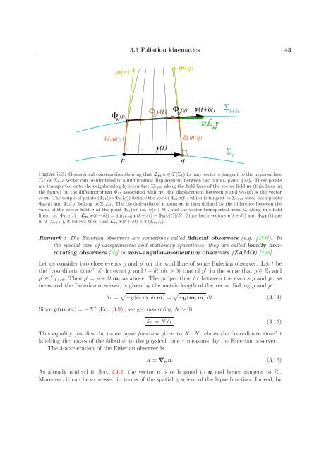
Figure 3.3: Geometrical construction showing that Lm v ∈ T (Σt) for any vector v tangent to the hypersurface
Σt: on Σt, a vector can be identified to a infinitesimal displacement between two points, p and q say. These points
are transported onto the neighbouring hypersurface Σt+δt along the field lines of the vector field m (thin lines on
the figure) by the diffeomorphism Φδt associated with m: the displacement between p and Φδt(p) is the vector
δtm. The couple of points (Φδt(p),Φδt(q)) defines the vector Φδtv(t), which is tangent to Σt+δt since both points
Φδt(p) and Φδt(q) belong to Σt+δt. The Lie derivative of v along m is then defined by the difference between the
value of the vector field v at the point Φδt(p), i.e. v(t + δt), and the vector transported from Σt along m’s field
lines, i.e. Φδtv(t) : Lm v(t + δt) = limδt→0[v(t + δt) − Φδtv(t)]/δt. Since both vectors v(t + δt) and Φδtv(t) are
in T (Σt+δt), it follows then that Lm v(t + δt) ∈ T (Σt+δt).
Remark : The Eulerian observers are sometimes called fiducial observers (e.g. [258]). In
the special case of axisymmetric and stationary spacetimes, they are called locally nonrotating
observers [34] or zero-angular-momentum observers (ZAMO) [258].
Let us consider two close events p and p ′ on the worldline of some Eulerian observer. Let t be
the “coordinate time” of the event p and t + δt (δt > 0) that of p ′ , in the sense that p ∈ Σt and
p ′ ∈ Σt+δt. Then p ′ = p + δt m, as above. The proper time δτ between the events p and p ′ , as
measured the Eulerian observer, is given by the metric length of the vector linking p and p ′ :
δτ = −g(δt m,δt m) = −g(m,m) δt. (3.14)
Since g(m,m) = −N 2 [Eq. (3.9)], we get (assuming N > 0)
δτ = N δt . (3.15)
This equality justifies the name lapse function given to N: N relates the “coordinate time” t
labelling the leaves of the foliation to the physical time τ measured by the Eulerian observer.
The 4-acceleration of the Eulerian observer is
a = ∇nn. (3.16)
As already noticed in Sec. 2.4.2, the vector a is orthogonal to n and hence tangent to Σt.
Moreover, it can be expressed in terms of the spatial gradient of the lapse function. Indeed, by