3+1 formalism and bases of numerical relativity - LUTh ...
3+1 formalism and bases of numerical relativity - LUTh ... 3+1 formalism and bases of numerical relativity - LUTh ...
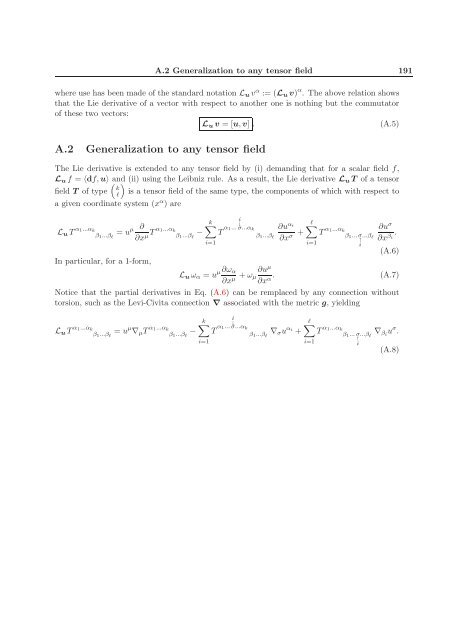
190 Lie derivative Figure A.1: Geometrical construction of the Lie derivative of a vector field: given a small parameter λ, each extremity of the arrow λv is dragged by some small parameter ε along u, to form the vector denoted by Φε(λv). The latter is then compared with the actual value of λv at the point q, the difference (divided by λε) defining the Lie derivative Lu v. Φε(p) of the point p by the transport by an infinitesimal “distance” ε along the field lines of u as Φε(p) = q, where q is the point close to p such that −→ pq = εu(p). Besides, if we multiply the vector v(p) by some infinitesimal parameter λ, it becomes an infinitesimal vector at p. Then there exists a unique point p ′ close to p such that λv(p) = −→ pp ′ . We may transport the point p ′ to a point q ′ along the field lines of u by the same “distance” ε as that used to transport p to q: q ′ = Φε(p ′ ) (see Fig. A.1). −→ qq ′ is then an infinitesimal vector at q and we define the transport by the distance ε of the vector v(p) along the field lines of u according to Φε(v(p)) := 1 −→ qq λ ′ . (A.1) Φε(v(p)) is vector in Tq(M). We may then subtract it from the actual value of the field v at q and define the Lie derivative of v along u by 1 Lu v := lim ε→0 ε [v(q) − Φε(v(p))] . (A.2) If we consider a coordinate system (xα ) adapted to the field u in the sense that u = e0 where e0 is the first vector of the natural basis associated with the coordinates (xα ), then the Lie derivative is simply given by the partial derivative of the vector components with respect to x0 : (Lu v) α = ∂vα . (A.3) ∂x0 In an arbitrary coordinate system, this formula is generalized to Lu v α = u µ∂vα − vµ∂uα , (A.4) ∂x µ ∂x µ
A.2 Generalization to any tensor field 191 where use has been made of the standard notation Lu v α := (Lu v) α . The above relation shows that the Lie derivative of a vector with respect to another one is nothing but the commutator of these two vectors: Lu v = [u,v] . (A.5) A.2 Generalization to any tensor field The Lie derivative is extended to any tensor field by (i) demanding that for a scalar field f, Lu f = 〈df,u〉 and (ii) using the Leibniz rule. As a result, the Lie derivative Lu T of a tensor k field T of type ℓ is a tensor field of the same type, the components of which with respect to a given coordinate system (x α ) are Lu T α1...αk β1...βℓ ∂ α1...αk = uµ ∂x µT β1...βℓ − k T α1... i=1 i ↓ σ...αk β1...βℓ ∂uαi + ∂xσ ℓ T α1...αk i=1 β1... σ...βℓ ↑ i ∂uσ . βi ∂x (A.6) In particular, for a 1-form, Luωα = u µ∂ωα ∂u + ωµ ∂x µ µ ∂xα. (A.7) Notice that the partial derivatives in Eq. (A.6) can be remplaced by any connection without torsion, such as the Levi-Civita connection ∇ associated with the metric g, yielding LuT α1...αk β1...βℓ = uµ ∇µT α1...αk β1...βℓ − k T α1... i=1 i ↓ σ...αk β1...βℓ ∇σu αi + ℓ T α1...αk i=1 β1... σ...βℓ ↑ i ∇βiuσ . (A.8)
- Page 140 and 141: 140 The initial data problem Accord
- Page 142 and 143: 142 The initial data problem Remark
- Page 144 and 145: 144 The initial data problem Remark
- Page 146 and 147: 146 The initial data problem 8.4.1
- Page 148 and 149: 148 The initial data problem Since
- Page 150 and 151: 150 The initial data problem • fo
- Page 152 and 153: 152 Choice of foliation and spatial
- Page 154 and 155: 154 Choice of foliation and spatial
- Page 156 and 157: 156 Choice of foliation and spatial
- Page 158 and 159: 158 Choice of foliation and spatial
- Page 160 and 161: 160 Choice of foliation and spatial
- Page 162 and 163: 162 Choice of foliation and spatial
- Page 164 and 165: 164 Choice of foliation and spatial
- Page 166 and 167: 166 Choice of foliation and spatial
- Page 168 and 169: 168 Choice of foliation and spatial
- Page 170 and 171: 170 Choice of foliation and spatial
- Page 172 and 173: 172 Choice of foliation and spatial
- Page 174 and 175: 174 Choice of foliation and spatial
- Page 176 and 177: 176 Evolution schemes been used by
- Page 178 and 179: 178 Evolution schemes Comparing wit
- Page 180 and 181: 180 Evolution schemes Now the ∇-d
- Page 182 and 183: 182 Evolution schemes coordinates (
- Page 184 and 185: 184 Evolution schemes = 1 2 −∆
- Page 186 and 187: 186 Evolution schemes corresponds t
- Page 188 and 189: 188 Evolution schemes
- Page 192 and 193: 192 Lie derivative
- Page 194 and 195: 194 Conformal Killing operator and
- Page 196 and 197: 196 Conformal Killing operator and
- Page 198 and 199: 198 Conformal Killing operator and
- Page 200 and 201: 200 BIBLIOGRAPHY [13] A. Anderson a
- Page 202 and 203: 202 BIBLIOGRAPHY [43] T.W. Baumgart
- Page 204 and 205: 204 BIBLIOGRAPHY [75] M. Campanelli
- Page 206 and 207: 206 BIBLIOGRAPHY [105] G. Darmois :
- Page 208 and 209: 208 BIBLIOGRAPHY [135] H. Friedrich
- Page 210 and 211: 210 BIBLIOGRAPHY [163] J. Isenberg
- Page 212 and 213: 212 BIBLIOGRAPHY [195] S. Nissanke
- Page 214 and 215: 214 BIBLIOGRAPHY [226] M. Shibata :
- Page 216 and 217: 216 BIBLIOGRAPHY [255] K. Taniguchi
- Page 218 and 219: Index 1+log slicing, 161 3+1 formal
- Page 220: 220 INDEX Ricci identity, 18 Ricci
A.2 Generalization to any tensor field 191<br />
where use has been made <strong>of</strong> the st<strong>and</strong>ard notation Lu v α := (Lu v) α . The above relation shows<br />
that the Lie derivative <strong>of</strong> a vector with respect to another one is nothing but the commutator<br />
<strong>of</strong> these two vectors:<br />
Lu v = [u,v] . (A.5)<br />
A.2 Generalization to any tensor field<br />
The Lie derivative is extended to any tensor field by (i) dem<strong>and</strong>ing that for a scalar field f,<br />
Lu f = 〈df,u〉 <strong>and</strong> (ii) using the Leibniz rule. As a result, the Lie derivative Lu <br />
T <strong>of</strong> a tensor<br />
k<br />
field T <strong>of</strong> type ℓ is a tensor field <strong>of</strong> the same type, the components <strong>of</strong> which with respect to<br />
a given coordinate system (x α ) are<br />
Lu T α1...αk<br />
β1...βℓ<br />
∂ α1...αk<br />
= uµ<br />
∂x µT β1...βℓ −<br />
k<br />
T α1...<br />
i=1<br />
i<br />
↓<br />
σ...αk<br />
β1...βℓ<br />
∂uαi +<br />
∂xσ ℓ<br />
T α1...αk<br />
i=1<br />
β1... σ...βℓ ↑<br />
i<br />
∂uσ . βi ∂x<br />
(A.6)<br />
In particular, for a 1-form,<br />
Luωα = u µ∂ωα ∂u<br />
+ ωµ<br />
∂x µ µ<br />
∂xα. (A.7)<br />
Notice that the partial derivatives in Eq. (A.6) can be remplaced by any connection without<br />
torsion, such as the Levi-Civita connection ∇ associated with the metric g, yielding<br />
LuT α1...αk<br />
β1...βℓ = uµ ∇µT α1...αk<br />
β1...βℓ −<br />
k<br />
T α1...<br />
i=1<br />
i<br />
↓<br />
σ...αk<br />
β1...βℓ ∇σu αi +<br />
ℓ<br />
T α1...αk<br />
i=1<br />
β1... σ...βℓ ↑<br />
i<br />
∇βiuσ .<br />
(A.8)


