3+1 formalism and bases of numerical relativity - LUTh ...

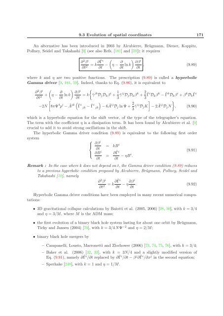
9.3 Evolution of spatial coordinates 171
An alternative has been introduced in 2003 by Alcubierre, Brügmann, Diener, Koppitz,
Pollney, Seidel and Takahashi [9] (see also Refs. [181] and [59]); it requires
∂2βi ∂t2 = k∂˜ Γi ∂t −
η − ∂
∂βi ln k
∂t ∂t
, (9.89)
where k and η are two positive functions. The prescription (9.89) is called a hyperbolic
Gamma driver [9, 181, 59]. Indeed, thanks to Eq. (9.86), it is equivalent to
∂2βi
+ η −
∂t2 ∂
∂βi ln k = k ˜γ
∂t ∂t jk DjDkβ i + 1
3 ˜γij DjDkβ k + 2
3 ˜ Γ i Dkβ k − ˜ Γ k Dkβ i + β k Dk ˜ Γ i
−2N 8πΨ 4 p i − Ãjk Γ˜ i
jk − ¯ Γ i
jk − 6ÃijDj ln Ψ + 2
3 ˜γij
DjK − 2Ãij
DjN , (9.90)
which is a hyperbolic equation for the shift vector, of the type of the telegrapher’s equation.
The term with the coefficient η is a dissipation term. It has been found by Alcubierre et al. [9]
crucial to add it to avoid strong oscillations in the shift.
The hyperbolic Gamma driver condition (9.89) is equivalent to the following first order
system
⎧
⎪⎨
⎪⎩
∂βi ∂t
= kBi
∂B i
∂t = ∂˜ Γ i
∂t − ηBi .
(9.91)
Remark : In the case where k does not depend on t, the Gamma driver condition (9.89) reduces
to a previous hyperbolic condition proposed by Alcubierre, Brügmann, Pollney, Seidel and
Takahashi [10], namely
∂2βi ∂t2 = k∂˜ Γi ∂t
− η∂βi . (9.92)
∂t
Hyperbolic Gamma driver conditions have been employed in many recent numerical computations:
• 3D gravitational collapse calculations by Baiotti et al. (2005, 2006) [28, 30], with k = 3/4
and η = 3/M, where M is the ADM mass;
• the first evolution of a binary black hole system lasting for about one orbit by Brügmann,
Tichy and Jansen (2004) [70], with k = 3/4NΨ −2 and η = 2/M;
• binary black hole mergers by
– Campanelli, Lousto, Marronetti and Zlochower (2006) [73, 74, 75, 76], with k = 3/4;
– Baker et al. (2006) [32, 33], with k = 3N/4 and a slightly modified version of
Eq. (9.91), namely ∂˜Γ i /∂t replaced by ∂˜Γ i /∂t − β j ∂˜Γ i /∂x j in the second equation;
– Sperhake [248], with k = 1 and η = 1/M.