3+1 formalism and bases of numerical relativity - LUTh ...
3+1 formalism and bases of numerical relativity - LUTh ... 3+1 formalism and bases of numerical relativity - LUTh ...
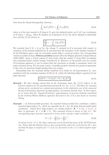
154 Choice of foliation and spatial coordinates Figure 9.2: Deformation of a volume V delimited by the surface S in the hypersurface Σ0. these coordinates does not depend upon t. The vector ∂t associated to these coordinates is then related to the displacement vector v by v = δt ∂t. (9.6) Introducing the lapse function N and shift vector β associated with the coordinates (t,x i ), the above relation becomes [cf. Eq. (4.31)] v = δt (Nn + β). Accordingly, the condition v| S = 0 implies N| S = 0 and β| S = 0. (9.7) Let us define V (t) as the volume of the domain Vt delimited by S in Σt. It is given by a formula identical to Eq. (9.5), except of course that the integration domain has to be replaced by Vt. Moreover, the domains Vt lying at fixed values of the coordinates (x i ), we have dV dt = Now, contracting Eq. (4.63) with γ ij and using Eq. (4.62), we get From the general rule (6.64) for the variation of a determinant, so that Eq. (9.9) becomes Vt ∂ √ γ ∂t d3 x. (9.8) ij ∂ γ ∂t γij = −2NK + 2Diβ i . (9.9) ij ∂ γ ∂t γij = ∂ 2 (ln γ) = √ ∂t γ ∂ √ γ , (9.10) ∂t 1 ∂ √ γ √ γ ∂t = −NK + Diβ i . (9.11) Let us use this relation to express Eq. (9.8) as dV dt = −NK + Diβ i √ 3 γ d x. (9.12) Vt
Now from the Gauss-Ostrogradsky theorem, Diβ i√ γ d 3 x = Vt 9.2 Choice of foliation 155 S β i √ 2 si q d y, (9.13) where s is the unit normal to S lying in Σt, q is the induced metric on S, (ya ) are coordinates on S and q = detqab. Since β vanishes on S [property (9.7)], the above integral is identically zero and Eq. (9.12) reduces to dV dt = − Vt NK √ γ d 3 x . (9.14) We conclude that if K = 0 on Σ0, the volume V enclosed in S is extremal with respect to variations of the domain delimited by S, provided that the boundary of the domain remains S. In the Euclidean space, such an extremum would define a minimal surface, the corresponding variation problem being a Plateau problem [named after the Belgian physicist Joseph Plateau (1801-1883)]: given a closed contour S (wire loop), find the surface V (soap film) of minimal area (minimal surface tension energy) bounded by S. However, in the present case of a metric of Lorentzian signature, it can be shown that the extremum is actually a maximum, hence the name maximal slicing. For the same reason, a timelike geodesic between two points in spacetime is the curve of maximum length joining these two points. Demanding that the maximal slicing condition (9.4) holds for all hypersurfaces Σt, once combined with the evolution equation (6.90) for K, yields the following elliptic equation for the lapse function: DiD i N = N 4π(E + S) + KijK ij . (9.15) Remark : We have already noticed that at the Newtonian limit, Eq. (9.15) reduces to the Poisson equation for the gravitational potential Φ (cf. Sec. 6.5.1). Therefore the maximal slicing can be considered as a natural generalization to the relativistic case of the canonical slicing of Newtonian spacetime by hypersurfaces of constant absolute time. In this respect, let us notice that the “beyond Newtonian” approximation of general relativity constituted by the Isenberg-Wilson-Mathews approach discussed in Sec. 6.6 is also based on maximal slicing. Example : In Schwarzschild spacetime, the standard Schwarzschild time coordinate t defines maximal hypersurfaces Σt, which are spacelike for R > 2m (R being Schwarzschild radial coordinate). Indeed these hypersurfaces are totally geodesic: K = 0 (cf. § 2.4.3), so that, in particular, K = trγK = 0. This maximal slicing is shown in Fig. 9.3. The corresponding lapse function expressed in terms of the isotropic radial coordinate r is N = 1 − m 1 + 2r m −1 . (9.16) 2r As shown in Sec. 8.3.3, the above expression can be derived by means of the XCTS formalism. Notice that the foliation (Σt)t∈R does not penetrate under the event horizon (R = 2m) and that the lapse is negative for r < m/2 (cf. discussion in Sec. 8.3.3 about negative lapse values).
- Page 104 and 105: 104 Asymptotic flatness and global
- Page 106 and 107: 106 Asymptotic flatness and global
- Page 108 and 109: 108 Asymptotic flatness and global
- Page 110 and 111: 110 Asymptotic flatness and global
- Page 112 and 113: 112 Asymptotic flatness and global
- Page 114 and 115: 114 Asymptotic flatness and global
- Page 116 and 117: 116 Asymptotic flatness and global
- Page 118 and 119: 118 Asymptotic flatness and global
- Page 120 and 121: 120 Asymptotic flatness and global
- Page 122 and 123: 122 Asymptotic flatness and global
- Page 124 and 125: 124 Asymptotic flatness and global
- Page 126 and 127: 126 The initial data problem Notice
- Page 128 and 129: 128 The initial data problem where
- Page 130 and 131: 130 The initial data problem 8.2.3
- Page 132 and 133: 132 The initial data problem where
- Page 134 and 135: 134 The initial data problem Figure
- Page 136 and 137: 136 The initial data problem Figure
- Page 138 and 139: 138 The initial data problem In par
- Page 140 and 141: 140 The initial data problem Accord
- Page 142 and 143: 142 The initial data problem Remark
- Page 144 and 145: 144 The initial data problem Remark
- Page 146 and 147: 146 The initial data problem 8.4.1
- Page 148 and 149: 148 The initial data problem Since
- Page 150 and 151: 150 The initial data problem • fo
- Page 152 and 153: 152 Choice of foliation and spatial
- Page 156 and 157: 156 Choice of foliation and spatial
- Page 158 and 159: 158 Choice of foliation and spatial
- Page 160 and 161: 160 Choice of foliation and spatial
- Page 162 and 163: 162 Choice of foliation and spatial
- Page 164 and 165: 164 Choice of foliation and spatial
- Page 166 and 167: 166 Choice of foliation and spatial
- Page 168 and 169: 168 Choice of foliation and spatial
- Page 170 and 171: 170 Choice of foliation and spatial
- Page 172 and 173: 172 Choice of foliation and spatial
- Page 174 and 175: 174 Choice of foliation and spatial
- Page 176 and 177: 176 Evolution schemes been used by
- Page 178 and 179: 178 Evolution schemes Comparing wit
- Page 180 and 181: 180 Evolution schemes Now the ∇-d
- Page 182 and 183: 182 Evolution schemes coordinates (
- Page 184 and 185: 184 Evolution schemes = 1 2 −∆
- Page 186 and 187: 186 Evolution schemes corresponds t
- Page 188 and 189: 188 Evolution schemes
- Page 190 and 191: 190 Lie derivative Figure A.1: Geom
- Page 192 and 193: 192 Lie derivative
- Page 194 and 195: 194 Conformal Killing operator and
- Page 196 and 197: 196 Conformal Killing operator and
- Page 198 and 199: 198 Conformal Killing operator and
- Page 200 and 201: 200 BIBLIOGRAPHY [13] A. Anderson a
- Page 202 and 203: 202 BIBLIOGRAPHY [43] T.W. Baumgart
Now from the Gauss-Ostrogradsky theorem,<br />
<br />
Diβ i√ γ d 3 <br />
x =<br />
Vt<br />
9.2 Choice <strong>of</strong> foliation 155<br />
S<br />
β i √ 2<br />
si q d y, (9.13)<br />
where s is the unit normal to S lying in Σt, q is the induced metric on S, (ya ) are coordinates<br />
on S <strong>and</strong> q = detqab. Since β vanishes on S [property (9.7)], the above integral is identically<br />
zero <strong>and</strong> Eq. (9.12) reduces to<br />
dV<br />
dt<br />
<br />
= −<br />
Vt<br />
NK √ γ d 3 x . (9.14)<br />
We conclude that if K = 0 on Σ0, the volume V enclosed in S is extremal with respect to<br />
variations <strong>of</strong> the domain delimited by S, provided that the boundary <strong>of</strong> the domain remains S.<br />
In the Euclidean space, such an extremum would define a minimal surface, the corresponding<br />
variation problem being a Plateau problem [named after the Belgian physicist Joseph Plateau<br />
(1801-1883)]: given a closed contour S (wire loop), find the surface V (soap film) <strong>of</strong> minimal<br />
area (minimal surface tension energy) bounded by S. However, in the present case <strong>of</strong> a metric<br />
<strong>of</strong> Lorentzian signature, it can be shown that the extremum is actually a maximum, hence the<br />
name maximal slicing. For the same reason, a timelike geodesic between two points in spacetime<br />
is the curve <strong>of</strong> maximum length joining these two points.<br />
Dem<strong>and</strong>ing that the maximal slicing condition (9.4) holds for all hypersurfaces Σt, once<br />
combined with the evolution equation (6.90) for K, yields the following elliptic equation for the<br />
lapse function:<br />
DiD i N = N 4π(E + S) + KijK ij . (9.15)<br />
Remark : We have already noticed that at the Newtonian limit, Eq. (9.15) reduces to the<br />
Poisson equation for the gravitational potential Φ (cf. Sec. 6.5.1). Therefore the maximal<br />
slicing can be considered as a natural generalization to the relativistic case <strong>of</strong> the canonical<br />
slicing <strong>of</strong> Newtonian spacetime by hypersurfaces <strong>of</strong> constant absolute time. In this respect,<br />
let us notice that the “beyond Newtonian” approximation <strong>of</strong> general <strong>relativity</strong> constituted<br />
by the Isenberg-Wilson-Mathews approach discussed in Sec. 6.6 is also based on maximal<br />
slicing.<br />
Example : In Schwarzschild spacetime, the st<strong>and</strong>ard Schwarzschild time coordinate t defines<br />
maximal hypersurfaces Σt, which are spacelike for R > 2m (R being Schwarzschild radial<br />
coordinate). Indeed these hypersurfaces are totally geodesic: K = 0 (cf. § 2.4.3), so<br />
that, in particular, K = trγK = 0. This maximal slicing is shown in Fig. 9.3. The<br />
corresponding lapse function expressed in terms <strong>of</strong> the isotropic radial coordinate r is<br />
<br />
N = 1 − m<br />
<br />
1 +<br />
2r<br />
m<br />
−1 . (9.16)<br />
2r<br />
As shown in Sec. 8.3.3, the above expression can be derived by means <strong>of</strong> the XCTS <strong>formalism</strong>.<br />
Notice that the foliation (Σt)t∈R does not penetrate under the event horizon (R = 2m)<br />
<strong>and</strong> that the lapse is negative for r < m/2 (cf. discussion in Sec. 8.3.3 about negative lapse<br />
values).


