3+1 formalism and bases of numerical relativity - LUTh ...

More documents

Recommendations

Info

142 The initial data problem Remark : The XCTS system (8.99)-(8.101) is a coupled system. Contrary to the CTT system (8.20)-(8.21), the assumption of constant mean curvature, and in particular of maximal slicing, does not allow to decouple it. 8.3.3 XCTS at work: static black hole example Let us illustrate the extended conformal thin sandwich method on a simple example. Take for the hypersurface Σ0 the punctured manifold considered in Sec. 8.2.6, namely For the free data, let us perform the simplest choice: Σ0 = R 3 \{O}. (8.102) ˜γij = fij, ˙˜γ ij = 0, K = 0, ˙ K = 0, ˜ E = 0, ˜ S = 0, and ˜p i = 0, (8.103) i.e. we are searching for vacuum initial data on a maximal and conformally flat hypersurface with all the freely specifiable time derivatives set to zero. Thanks to (8.103), the XCTS system (8.99)-(8.101) reduces to Aiming at finding the simplest solution, we notice that ∆Ψ + 1 8 Âij Âij Ψ −7 = 0 (8.104) 1 Dj Ñ (Lβ)ij = 0 (8.105) ∆( ÑΨ7 ) − 7 8 Âij Âij Ψ −1 Ñ = 0. (8.106) β = 0 (8.107) is a solution of Eq. (8.105). Together with ˙˜γ ij = 0, it leads to [cf. Eq. (8.90)] The system (8.104)-(8.106) reduces then further: Â ij = 0. (8.108) ∆Ψ = 0 (8.109) ∆( ÑΨ7 ) = 0. (8.110) Hence we have only two Laplace equations to solve. Moreover Eq. (8.109) decouples from Eq. (8.110). For simplicity, let us assume spherical symmetry around the puncture O. We introduce an adapted spherical coordinate system (xi ) = (r,θ,ϕ) on Σ0. The puncture O is then at r = 0. The simplest non-trivial solution of (8.109) which obeys the asymptotic flatness condition Ψ → 1 as r → +∞ is Ψ = 1 + m , (8.111) 2r where as in Sec. 8.2.5, the constant m is the ADM mass of Σ0 [cf. Eq. (8.61)]. Notice that since r = 0 is excluded from Σ0, Ψ is a perfectly regular solution on the entire manifold Σ0. Let us
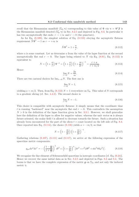
8.3 Conformal thin sandwich method 143 recall that the Riemannian manifold (Σ0,γ) corresponding to this value of Ψ via γ = Ψ4f is the Riemannian manifold denoted (Σ ′ 0 ,γ) in Sec. 8.2.5 and depicted in Fig. 8.3. In particular it has two asymptotically flat ends: r → +∞ and r → 0 (the puncture). As for Eq. (8.109), the simplest solution of Eq. (8.110) obeying the asymptotic flatness requirement ÑΨ7 → 1 as r → +∞ is ÑΨ 7 = 1 + a , (8.112) r where a is some constant. Let us determine a from the value of the lapse function at the second asymptotically flat end r → 0. The lapse being related to Ñ via Eq. (8.91), Eq. (8.112) is equivalent to N = 1 + a Ψ r −1 = 1 + a 1 + r m −1 = 2r r + a . (8.113) r + m/2 Hence 2a lim N = . r→0 m (8.114) There are two natural choices for limr→0 N. The first one is lim N = 1, (8.115) r→0 yielding a = m/2. Then, from Eq. (8.113) N = 1 everywhere on Σ0. This value of N corresponds to a geodesic slicing (cf. Sec. 4.4.2). The second choice is lim N = −1. (8.116) r→0 This choice is compatible with asymptotic flatness: it simply means that the coordinate time t is running “backward” near the asymptotic flat end r → 0. This contradicts the assumption N > 0 in the definition of the lapse function given in Sec. 3.3.1. However, we shall generalize here the definition of the lapse to allow for negative values: whereas the unit vector n is always future-oriented, the scalar field t is allowed to decrease towards the future. Such a situation has already been encountered for the part of the slices t = const located on the left side of Fig. 8.4. Once reported into Eq. (8.114), the choice (8.116) yields a = −m/2, so that N = 1 − m 1 + 2r m −1 . (8.117) 2r Gathering relations (8.107), (8.111) and (8.117), we arrive at the following expression of the spacetime metric components: gµνdx µ dx ν m 1 − 2r = − 1 + m 2 dt 2r 2 + 1 + m 4 dr 2 2 2 2 2 + r (dθ + sin θdϕ ) . (8.118) 2r We recognize the line element of Schwarzschild spacetime in isotropic coordinates [cf. Eq. (6.24)]. Hence we recover the same initial data as in Sec. 8.2.5 and depicted in Figs. 8.3 and 8.4. The bonus is that we have the complete expression of the metric g on Σ0, and not only the induced metric γ.
Page 1:
arXiv:gr-qc/0703035v1 6 Mar 2007 3+
Page 4 and 5:
4 CONTENTS 3.3.6 Evolution of the o
Page 6 and 7:
6 CONTENTS 8 The initial data probl
Page 8 and 9:
8 CONTENTS
Page 10 and 11:
10 CONTENTS
Page 12 and 13:
12 Introduction 3D (no symmetry at
Page 14 and 15:
14 Introduction
Page 16 and 17:
16 Geometry of hypersurfaces in two
Page 18 and 19:
18 Geometry of hypersurfaces 2.2.3
Page 20 and 21:
20 Geometry of hypersurfaces Figure
Page 22 and 23:
22 Geometry of hypersurfaces •
Page 24 and 25:
24 Geometry of hypersurfaces The ei
Page 26 and 27:
26 Geometry of hypersurfaces Figure
Page 28 and 29:
28 Geometry of hypersurfaces The no
Page 30 and 31:
30 Geometry of hypersurfaces Since
Page 32 and 33:
32 Geometry of hypersurfaces 2.4.3
Page 34 and 35:
34 Geometry of hypersurfaces 2.5 Ga
Page 36 and 37:
36 Geometry of hypersurfaces Exampl
Page 38 and 39:
38 Geometry of hypersurfaces
Page 40 and 41:
40 Geometry of foliations Figure 3.
Page 42 and 43:
42 Geometry of foliations 3.3.2 Nor
Page 44 and 45:
44 Geometry of foliations means Eq.
Page 46 and 47:
46 Geometry of foliations Remark :
Page 48 and 49:
48 Geometry of foliations Note that
Page 50 and 51:
50 Geometry of foliations
Page 52 and 53:
52 3+1 decomposition of Einstein eq
Page 54 and 55:
Page 56 and 57:
Page 58 and 59:
Page 60 and 61:
Page 62 and 63:
Page 64 and 65:
Page 66 and 67:
Page 68 and 69:
Page 70 and 71:
Page 72 and 73:
72 3+1 equations for matter and ele
Page 74 and 75:
Page 76 and 77:
Page 78 and 79:
Page 80 and 81:
Page 82 and 83:
Page 84 and 85:
84 Conformal decomposition equivale
Page 86 and 87:
86 Conformal decomposition As an ex
Page 88 and 89:
88 Conformal decomposition 6.2.4 Co
Page 90 and 91:
90 Conformal decomposition 6.3.1 Ge
Page 92 and 93: 92 Conformal decomposition where K
Page 94 and 95: 94 Conformal decomposition to write
Page 96 and 97: 96 Conformal decomposition hence Lm
Page 98 and 99: 98 Conformal decomposition 6.5.2 Ha
Page 100 and 101: 100 Conformal decomposition discuss
Page 102 and 103: 102 Conformal decomposition Remark
Page 104 and 105: 104 Asymptotic flatness and global
Page 126 and 127: 126 The initial data problem Notice
Page 128 and 129: 128 The initial data problem where
Page 130 and 131: 130 The initial data problem 8.2.3
Page 132 and 133: 132 The initial data problem where
Page 134 and 135: 134 The initial data problem Figure
Page 136 and 137: 136 The initial data problem Figure
Page 138 and 139: 138 The initial data problem In par
Page 140 and 141: 140 The initial data problem Accord
Page 144 and 145: 144 The initial data problem Remark
Page 146 and 147: 146 The initial data problem 8.4.1
Page 148 and 149: 148 The initial data problem Since
Page 150 and 151: 150 The initial data problem • fo
Page 152 and 153: 152 Choice of foliation and spatial
Page 176 and 177: 176 Evolution schemes been used by
Page 178 and 179: 178 Evolution schemes Comparing wit
Page 180 and 181: 180 Evolution schemes Now the ∇-d
Page 182 and 183: 182 Evolution schemes coordinates (
Page 184 and 185: 184 Evolution schemes = 1 2 −∆
Page 186 and 187: 186 Evolution schemes corresponds t
Page 188 and 189: 188 Evolution schemes
Page 190 and 191: 190 Lie derivative Figure A.1: Geom
Page 192 and 193:
192 Lie derivative
Page 194 and 195:
194 Conformal Killing operator and
Page 196 and 197:
Page 198 and 199:
Page 200 and 201:
200 BIBLIOGRAPHY [13] A. Anderson a
Page 202 and 203:
202 BIBLIOGRAPHY [43] T.W. Baumgart
Page 204 and 205:
204 BIBLIOGRAPHY [75] M. Campanelli
Page 206 and 207:
206 BIBLIOGRAPHY [105] G. Darmois :
Page 208 and 209:
208 BIBLIOGRAPHY [135] H. Friedrich
Page 210 and 211:
210 BIBLIOGRAPHY [163] J. Isenberg
Page 212 and 213:
212 BIBLIOGRAPHY [195] S. Nissanke
Page 214 and 215:
214 BIBLIOGRAPHY [226] M. Shibata :
Page 216 and 217:
216 BIBLIOGRAPHY [255] K. Taniguchi
Page 218 and 219:
Index 1+log slicing, 161 3+1 formal
Page 220:
220 INDEX Ricci identity, 18 Ricci
show all

3+1 formalism and bases of numerical relativity - LUTh ...

Create successful ePaper yourself

Delete template?

Save as template?