3+1 formalism and bases of numerical relativity - LUTh ...
3+1 formalism and bases of numerical relativity - LUTh ... 3+1 formalism and bases of numerical relativity - LUTh ...
114 Asymptotic flatness and global quantities turns out to be true in practice, as we shall see on the specific example of Kerr spacetime in Sec. 7.6.3. 7.5.2 The “cure” In view of the above coordinate dependence problem, one may define the angular momentum as a quantity which remains invariant only with respect to a subclass of the coordinate changes (7.7). This is made by imposing decay conditions stronger than (7.1)-(7.4). For instance, York [276] has proposed the following conditions 3 on the flat divergence of the conformal metric and the trace of the extrinsic curvature: ∂˜γij ∂x j = O(r−3 ), (7.64) K = O(r −3 ). (7.65) Clearly these conditions are stronger than respectively (7.35) and (7.3). Actually they are so severe that they exclude some well known coordinates that one would like to use to describe asymptotically flat spacetimes, for instance the standard Schwarzschild coordinates (7.16) for the Schwarzschild solution. For this reason, conditions (7.64) and (7.65) are considered as asymptotic gauge conditions, i.e. conditions restricting the choice of coordinates, rather than conditions on the nature of spacetime at spatial infinity. Condition (7.64) is called the quasi-isotropic gauge. The isotropic coordinates (6.24) of the Schwarzschild solution trivially belong to this gauge (since ˜γij = fij for them). Condition (7.65) is called the asymptotically maximal gauge, since for maximal hypersurfaces K vanishes identically. York has shown that in the gauge (7.64)-(7.65), the angular momentum as defined by the integral (7.63) is carried by the O(r −3 ) piece of K (the O(r −2 ) piece carrying the linear momentum Pi) and is invariant (i.e. behaves as a vector) for any coordinate change within this gauge. Alternative decay requirements have been proposed by other authors to fix the ambiguities in the angular momentum definition (see e.g. [92] and references therein). For instance, Regge and Teitelboim [209] impose a specific form and some parity conditions on the coefficient of the O(r −1 ) term in Eq. (7.1) and on the coefficient of the O(r −2 ) term in Eq. (7.3) (cf. also M. Henneaux’ lecture [157]). As we shall see in Sec. 7.6.3, in the particular case of an axisymmetric spacetime, there exists a unique definition of the angular momentum, which is independent of any coordinate system. Remark : In the literature, there is often mention of the “ADM angular momentum”, on the same footing as the ADM mass and ADM linear momentum. But as discussed above, there is no such thing as the “ADM angular momentum”. One has to specify a gauge first and define the angular momentum within that gauge. In particular, there is no mention whatsoever of angular momentum in the original ADM article [23]. 3 Actually the first condition proposed by York, Eq. (90) of Ref. [276], is not exactly (7.64) but can be shown to be equivalent to it; see also Sec. V of Ref. [246].
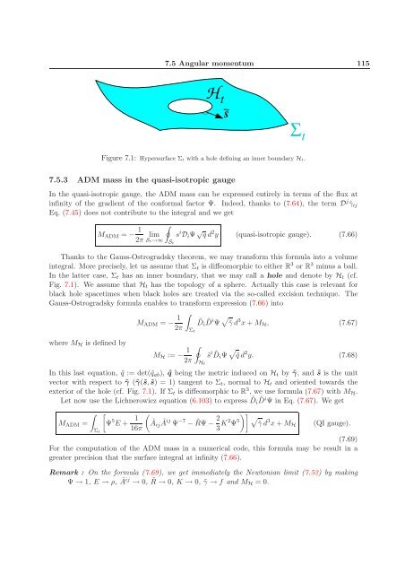
7.5 Angular momentum 115 Figure 7.1: Hypersurface Σt with a hole defining an inner boundary Ht. 7.5.3 ADM mass in the quasi-isotropic gauge In the quasi-isotropic gauge, the ADM mass can be expressed entirely in terms of the flux at infinity of the gradient of the conformal factor Ψ. Indeed, thanks to (7.64), the term D j ˜γij Eq. (7.45) does not contribute to the integral and we get MADM = − 1 2π lim s St→∞ St i DiΨ √ q d 2 y (quasi-isotropic gauge). (7.66) Thanks to the Gauss-Ostrogradsky theorem, we may transform this formula into a volume integral. More precisely, let us assume that Σt is diffeomorphic to either R 3 or R 3 minus a ball. In the latter case, Σt has an inner boundary, that we may call a hole and denote by Ht (cf. Fig. 7.1). We assume that Ht has the topology of a sphere. Actually this case is relevant for black hole spacetimes when black holes are treated via the so-called excision technique. The Gauss-Ostrogradsky formula enables to transform expression (7.66) into MADM = − 1 2π ˜Di ˜ D i Ψ ˜γ d 3 x + MH, (7.67) where MH is defined by Σt MH := − 1 ˜s 2π Ht i DiΨ ˜ ˜q d 2 y. (7.68) In this last equation, ˜q := det(˜qab), ˜q being the metric induced on Ht by ˜γ, and ˜s is the unit vector with respect to ˜γ (˜γ(˜s, ˜s) = 1) tangent to Σt, normal to Ht and oriented towards the exterior of the hole (cf. Fig. 7.1). If Σt is diffeomorphic to R 3 , we use formula (7.67) with MH. Let now use the Lichnerowicz equation (6.103) to express ˜ Di ˜ D i Ψ in Eq. (7.67). We get MADM = Σt Ψ 5 E + 1 Âij 16π Âij Ψ −7 − ˜ RΨ − 2 3 K2Ψ 5 ˜γ 3 d x + MH (QI gauge). (7.69) For the computation of the ADM mass in a numerical code, this formula may be result in a greater precision that the surface integral at infinity (7.66). Remark : On the formula (7.69), we get immediately the Newtonian limit (7.52) by making Ψ → 1, E → ρ, Âij → 0, ˜ R → 0, K → 0, ˜γ → f and MH = 0.
- Page 64 and 65: 64 3+1 decomposition of Einstein eq
- Page 66 and 67: 66 3+1 decomposition of Einstein eq
- Page 68 and 69: 68 3+1 decomposition of Einstein eq
- Page 70 and 71: 70 3+1 decomposition of Einstein eq
- Page 72 and 73: 72 3+1 equations for matter and ele
- Page 74 and 75: 74 3+1 equations for matter and ele
- Page 76 and 77: 76 3+1 equations for matter and ele
- Page 78 and 79: 78 3+1 equations for matter and ele
- Page 80 and 81: 80 3+1 equations for matter and ele
- Page 82 and 83: 82 3+1 equations for matter and ele
- Page 84 and 85: 84 Conformal decomposition equivale
- Page 86 and 87: 86 Conformal decomposition As an ex
- Page 88 and 89: 88 Conformal decomposition 6.2.4 Co
- Page 90 and 91: 90 Conformal decomposition 6.3.1 Ge
- Page 92 and 93: 92 Conformal decomposition where K
- Page 94 and 95: 94 Conformal decomposition to write
- Page 96 and 97: 96 Conformal decomposition hence Lm
- Page 98 and 99: 98 Conformal decomposition 6.5.2 Ha
- Page 100 and 101: 100 Conformal decomposition discuss
- Page 102 and 103: 102 Conformal decomposition Remark
- Page 104 and 105: 104 Asymptotic flatness and global
- Page 106 and 107: 106 Asymptotic flatness and global
- Page 108 and 109: 108 Asymptotic flatness and global
- Page 110 and 111: 110 Asymptotic flatness and global
- Page 112 and 113: 112 Asymptotic flatness and global
- Page 116 and 117: 116 Asymptotic flatness and global
- Page 118 and 119: 118 Asymptotic flatness and global
- Page 120 and 121: 120 Asymptotic flatness and global
- Page 122 and 123: 122 Asymptotic flatness and global
- Page 124 and 125: 124 Asymptotic flatness and global
- Page 126 and 127: 126 The initial data problem Notice
- Page 128 and 129: 128 The initial data problem where
- Page 130 and 131: 130 The initial data problem 8.2.3
- Page 132 and 133: 132 The initial data problem where
- Page 134 and 135: 134 The initial data problem Figure
- Page 136 and 137: 136 The initial data problem Figure
- Page 138 and 139: 138 The initial data problem In par
- Page 140 and 141: 140 The initial data problem Accord
- Page 142 and 143: 142 The initial data problem Remark
- Page 144 and 145: 144 The initial data problem Remark
- Page 146 and 147: 146 The initial data problem 8.4.1
- Page 148 and 149: 148 The initial data problem Since
- Page 150 and 151: 150 The initial data problem • fo
- Page 152 and 153: 152 Choice of foliation and spatial
- Page 154 and 155: 154 Choice of foliation and spatial
- Page 156 and 157: 156 Choice of foliation and spatial
- Page 158 and 159: 158 Choice of foliation and spatial
- Page 160 and 161: 160 Choice of foliation and spatial
- Page 162 and 163: 162 Choice of foliation and spatial
7.5 Angular momentum 115<br />
Figure 7.1: Hypersurface Σt with a hole defining an inner boundary Ht.<br />
7.5.3 ADM mass in the quasi-isotropic gauge<br />
In the quasi-isotropic gauge, the ADM mass can be expressed entirely in terms <strong>of</strong> the flux at<br />
infinity <strong>of</strong> the gradient <strong>of</strong> the conformal factor Ψ. Indeed, thanks to (7.64), the term D j ˜γij<br />
Eq. (7.45) does not contribute to the integral <strong>and</strong> we get<br />
MADM = − 1<br />
2π lim<br />
<br />
s<br />
St→∞ St<br />
i DiΨ √ q d 2 y (quasi-isotropic gauge). (7.66)<br />
Thanks to the Gauss-Ostrogradsky theorem, we may transform this formula into a volume<br />
integral. More precisely, let us assume that Σt is diffeomorphic to either R 3 or R 3 minus a ball.<br />
In the latter case, Σt has an inner boundary, that we may call a hole <strong>and</strong> denote by Ht (cf.<br />
Fig. 7.1). We assume that Ht has the topology <strong>of</strong> a sphere. Actually this case is relevant for<br />
black hole spacetimes when black holes are treated via the so-called excision technique. The<br />
Gauss-Ostrogradsky formula enables to transform expression (7.66) into<br />
MADM = − 1<br />
<br />
2π<br />
˜Di ˜ D i Ψ ˜γ d 3 x + MH, (7.67)<br />
where MH is defined by<br />
Σt<br />
MH := − 1<br />
<br />
˜s<br />
2π Ht<br />
i DiΨ ˜ ˜q d 2 y. (7.68)<br />
In this last equation, ˜q := det(˜qab), ˜q being the metric induced on Ht by ˜γ, <strong>and</strong> ˜s is the unit<br />
vector with respect to ˜γ (˜γ(˜s, ˜s) = 1) tangent to Σt, normal to Ht <strong>and</strong> oriented towards the<br />
exterior <strong>of</strong> the hole (cf. Fig. 7.1). If Σt is diffeomorphic to R 3 , we use formula (7.67) with MH.<br />
Let now use the Lichnerowicz equation (6.103) to express ˜ Di ˜ D i Ψ in Eq. (7.67). We get<br />
<br />
MADM =<br />
Σt<br />
<br />
Ψ 5 E + 1<br />
<br />
Âij<br />
16π<br />
Âij Ψ −7 − ˜ RΨ − 2<br />
3 K2Ψ 5<br />
<br />
˜γ<br />
3<br />
d x + MH<br />
(QI gauge).<br />
(7.69)<br />
For the computation <strong>of</strong> the ADM mass in a <strong>numerical</strong> code, this formula may be result in a<br />
greater precision that the surface integral at infinity (7.66).<br />
Remark : On the formula (7.69), we get immediately the Newtonian limit (7.52) by making<br />
Ψ → 1, E → ρ, Âij → 0, ˜ R → 0, K → 0, ˜γ → f <strong>and</strong> MH = 0.


