Gravitational Waves from Inspiralling Compact Binaries in ... - LUTH

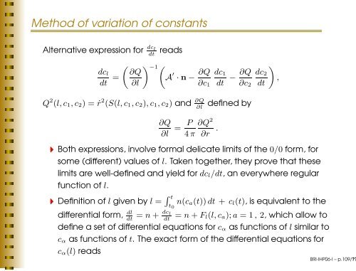
Method of variation of constants
Alternative expression for dc l
dt reads
dcl
dt =
∂Q
∂l
−1
A ′ · n − ∂Q
Q 2 (l, c1, c2) = ˙r 2 (S(l, c1, c2), c1, c2) and ∂Q
∂l
∂Q
∂l
= P
4 π
∂c1
dc1
dt
− ∂Q
∂c2
defined by
∂Q 2
∂r .
Both expressions, involve formal delicate limits of the 0/0 form, for
some (different) values of l. Taken together, they prove that these
limits are well-defined and yield for dcl/dt, an everywhere regular
function of l.
Definition of l given by l = t
t0 n(ca(t)) dt + cl(t), is equivalent to the
differential form, dl
dt = n + dcl dt = n + Fl(l, ca); a = 1 , 2, which allow to
define a set of differential equations for cα as functions of l similar to
cα as functions of t. The exact form of the differential equations for
cα(l) reads
dc2
dt
,
BRI-IHP06-I – p.109/??