- Page 1 and 2:
SENSORLESS FIELD ORIENTED CONTROL O
- Page 3 and 4:
Table of Contents List of Figures..
- Page 5 and 6:
CHAPTER 5 - Field Oriented Control
- Page 7 and 8:
List of Figures Figure 2.1 - Radial
- Page 9 and 10:
Figure 3.29 - Arbitrary space vecto
- Page 11 and 12:
Figure 4.44 - ZS components of some
- Page 13 and 14:
Figure C.13 - Single-turn full-pitc
- Page 15 and 16:
List of Symbols Symbol Meaning Unit
- Page 17 and 18:
Abbreviations ACIM AC induction mot
- Page 19 and 20:
Superscripts * commanded value ref
- Page 21 and 22:
CHAPTER 1 - Introduction Historical
- Page 23 and 24:
vector theory to model a machine, w
- Page 25 and 26:
publications and magazines, and Int
- Page 27 and 28:
elationship between SVM and other P
- Page 29 and 30:
CHAPTER 2 - Fundamentals of Electri
- Page 31 and 32:
Preliminaries In reading the litera
- Page 33 and 34:
Taxonomy of Motors There is any num
- Page 35 and 36:
characteristics (the DC load curren
- Page 37 and 38:
torque component, sturdily construc
- Page 39 and 40:
Figure 2.7 - Cross sections of some
- Page 41 and 42:
draw the line between the solenoida
- Page 43 and 44:
These texts generally attribute the
- Page 45 and 46:
N B A B Y x(t) (2.6) The induc
- Page 47 and 48:
extended to the rotational case lat
- Page 49 and 50:
present analysis). When this is tru
- Page 51 and 52:
Figure 2.16 - Components of total f
- Page 53 and 54:
As aforementioned a spatial analysi
- Page 55 and 56:
clear the meaning, but the reader i
- Page 57 and 58:
Figure 2.20 - Elementary brushless
- Page 59 and 60:
called the per-phase torque functio
- Page 61 and 62:
Expressing bEMF in terms of the bEM
- Page 63 and 64:
Equation (2.44) is the component of
- Page 65 and 66:
d R( r) ke( r) kt( r) sin( r) (2.
- Page 67 and 68:
General Electromechanical Models Th
- Page 69 and 70:
Figure 2.28 - Phase-variable simula
- Page 71 and 72:
Trapezoidal and Sinusoidal BPMS Mot
- Page 73 and 74:
Figure 2.29 - Back-EMF and drive cu
- Page 75 and 76: Figure 2.31 - Back-EMF and drive cu
- Page 77 and 78: 3 KT Ke 2 (sinusoidal) K 2 K (tra
- Page 79 and 80: control scheme must keep sinusoidal
- Page 81 and 82: with misconceptions. The primary is
- Page 83 and 84: Part I - Sinusoidal BPMS Motors wit
- Page 85 and 86: grounded-neutral wye or delta conne
- Page 87 and 88: N e f A ( ) i 2 N e f B ( ) i 2
- Page 89 and 90: Figure 3.7 - Developed view at zero
- Page 91 and 92: Figure 3.9 - Developed view showing
- Page 93 and 94: Although Equations (3.6) or (3.7) a
- Page 95 and 96: direction. The contributions always
- Page 97 and 98: sinusoidal electrical variable will
- Page 99 and 100: Figure 3.14 - Cross section of two
- Page 101 and 102: 3 N e (3.6): f ( , t) I p cos(
- Page 103 and 104: In the previous chapter the per-pha
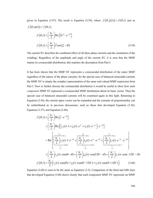
- Page 105 and 106: peak value is represented as an upp
- Page 107 and 108: Figure 3.21 - Time relationship bet
- Page 109 and 110: another and thus could be placed in
- Page 111 and 112: more widely understood theory (such
- Page 113 and 114: other methods, although it has clos
- Page 115 and 116: The SV as a Vector The first facet
- Page 117 and 118: j0 j0 j0 aˆ 1 0 1 bˆ j e e e
- Page 119 and 120: j j ee 1 cos( ) (3.45) 2 3 j t x
- Page 121 and 122: Notice that the amplitude of the MM
- Page 123 and 124: Figure 3.27 - Equivalent MMF produc
- Page 125: Ne 1 jj f , t i e i * e 2 2
- Page 129 and 130: 3 Ne j t f Ie p 2 2 . This
- Page 131 and 132: j set θ to anything. Taking the re
- Page 133 and 134: epresent any physically-distributed
- Page 135 and 136: lumped-parameter model in this repo
- Page 137 and 138: x kCx (3.75) abc The set of varia
- Page 139 and 140: phase variable axes; three axes in
- Page 141 and 142: The component MMFs act away from th
- Page 143 and 144: common choice is to force the power
- Page 145 and 146: As an example, find the SV that cor
- Page 147 and 148: the same magnitude, the projection
- Page 149 and 150: Figure 3.32 - Arbitrary SV referenc
- Page 151 and 152: universal and the choice of convent
- Page 153 and 154: stator’s perspective and at R fr
- Page 155 and 156: The potential discrepancy (p.108) w
- Page 157 and 158: x cos( r) sin( r) xd x sin(
- Page 159 and 160: It must be emphasized that we have
- Page 161 and 162: in relative time like an oscillogra
- Page 163 and 164: Part III - SV Theory Applied to Sin
- Page 165 and 166: In Equation (3.135) Z has elements
- Page 167 and 168: to use SV theory. It may be helpful
- Page 169 and 170: Figure 3.42 - Coupling between d- a
- Page 171 and 172: R R d R R v Ri Li j Li dt s
- Page 173 and 174: current does not influence the valu
- Page 175 and 176: d v Ri L i e dt d v Ri L i e
- Page 177 and 178:
Figure 3.47 - Simulation diagram fo
- Page 179 and 180:
e je ), and (2) it was demonstrate
- Page 181 and 182:
Overview of Voltage Source Inverter
- Page 183 and 184:
In addition to measuring voltages w
- Page 185 and 186:
then there would be periods during
- Page 187 and 188:
Figure 4.9 - Gating and POLE voltag
- Page 189 and 190:
Figure 4.11 - Ideal voltage wavefor
- Page 191 and 192:
inverter is called sine-triangle co
- Page 193 and 194:
and it offers the fastest dynamic r
- Page 195 and 196:
Figure 4.18 - Fundamental gain and
- Page 197 and 198:
In the literature this is called th
- Page 199 and 200:
voltage will be below (above) the b
- Page 201 and 202:
Figure 4.24 - Instantaneous phase-A
- Page 203 and 204:
Figure 4.26 - Base SVs showing the
- Page 205 and 206:
Figure 4.27 - Transformed voltage w
- Page 207 and 208:
also correspond to six-step squarew
- Page 209 and 210:
was fed to the SVM inverter as a SV
- Page 211 and 212:
Figure 4.31 - Temporal limit of inv
- Page 213 and 214:
Figure 4.34 - SVM overmodulation re
- Page 215 and 216:
Checking sextant s 23 again for thi
- Page 217 and 218:
SVM Implementation The block diagra
- Page 219 and 220:
has been made of using THI in the S
- Page 221 and 222:
different triplen signal would be i
- Page 223 and 224:
Similarly, when the modulation inde
- Page 225 and 226:
Summary and Conclusion The two-leve
- Page 227 and 228:
CHAPTER 5 - Field Oriented Control
- Page 229 and 230:
torque production; this is called d
- Page 231 and 232:
Figure 5.3 - Torque control of sinu
- Page 233 and 234:
obviously a change in perspective.
- Page 235 and 236:
Figure 5.9 - Comparison of referenc
- Page 237 and 238:
variables to the stationary referen
- Page 239 and 240:
Figure 5.13 - Torque control of sin
- Page 241 and 242:
To analyze a salient machine one mu
- Page 243 and 244:
Figure 5.16 - Torque functions: (a)
- Page 245 and 246:
Figure 5.19 - Buried permanent magn
- Page 247 and 248:
Figure 5.21 - Flux weakening in the
- Page 249 and 250:
appears that this is very much rela
- Page 251 and 252:
Stationary and Synchronous Regulato
- Page 253 and 254:
stationary regulator had. For compl
- Page 255 and 256:
This coupling can be mitigated by m
- Page 257 and 258:
educes to two independent circuits,
- Page 259 and 260:
D, some of the 120° methods are ap
- Page 261 and 262:
d d v Ri Ls i R dt dt The r
- Page 263 and 264:
section a state-space model for the
- Page 265 and 266:
Figure 6.6 - Full state feedback (o
- Page 267 and 268:
State-Space Model of BPMS Motor A s
- Page 269 and 270:
Figure 6.9 - FOC block diagram. The
- Page 271 and 272:
loop). A second way to implement th
- Page 273 and 274:
knowing the rotor position from ini
- Page 275 and 276:
[11] E. Clarke, Circuit analysis of
- Page 277 and 278:
Control Systems, Linear Analysis [4
- Page 279 and 280:
[77] J.M.D. Murphy, F.G. Turnbull,
- Page 281 and 282:
Machine Modeling, Analysis [103] J.
- Page 283 and 284:
THI, SVM, SPWM [127] J.A. Houldswor
- Page 285 and 286:
Wisconsin-Madison. [Online]. Availa
- Page 287 and 288:
Angle Tracking [175] D. Morgan, “
- Page 289 and 290:
Appendix A - Elementary Electromagn
- Page 291 and 292:
L i (A.8) S SS S SR S SS SR (A.9
- Page 293 and 294:
First the self-flux-linkage of an i
- Page 295 and 296:
vAN R iA LM iA eA d v R i
- Page 297 and 298:
Figure B.3 - One-half of the flux p
- Page 299 and 300:
Equations (B.27) and (B.28) are for
- Page 301 and 302:
Fundamental Relationships Figure C.
- Page 303 and 304:
Figure C.3 - Sinusoidal winding den
- Page 305 and 306:
manufactured compared to the steppe
- Page 307 and 308:
phase winding of Figure C.4 will ha
- Page 309 and 310:
Distributed N Fp i 2 (C.5) Figu
- Page 311 and 312:
alanced machine only odd harmonics
- Page 313 and 314:
sinusoidal windings with a sinusoid
- Page 315 and 316:
0, and since the direction of inte
- Page 317 and 318:
That the rotor-stator flux linkage
- Page 319 and 320:
Figure C.17 - Summary of rotor-stat
- Page 321 and 322:
Figure C.19 - Amplitudes of harmoni
- Page 323 and 324:
triangle with an amplitude whose nu
- Page 325 and 326:
Returning to Figure C.18 it is clea
- Page 327 and 328:
torque will describe the torque pro
- Page 329 and 330:
However, Equation (D.2) is incorrec
- Page 331 and 332:
the same order as the PS set (arran
- Page 333 and 334:
Implications of the ZS Component Th
- Page 335 and 336:
Figure D.6 - Neutral voltage of loa
- Page 337 and 338:
3v 3e 3v v v v v v v 3v AM BM CM A
- Page 339 and 340:
components of source voltage sum to
- Page 341 and 342:
Equation (D.25) and instantaneous q
- Page 343 and 344:
If a ZS component could possibly be
- Page 345 and 346:
xA X1cos( t) X3cos(3 t) X5cos(5 t)
- Page 347 and 348:
Figure D.11 - 3-D base vectors of 1
- Page 349 and 350:
the Clarke transform is used. Howev
- Page 351 and 352:
Appendix E - Park Transforms This a
- Page 353 and 354:
Appendix F - Useful Mathematical Re
- Page 355:
335