Status of inflation - KICP Workshops

Status of inflation 



Marco Peloso, 

Marco Peloso, University of Minnesota 

Gumrukcuoglu, Contaldi, MP, JCAP ’07 

Marco Peloso, University Universityof of Minnesota 

University of Minnesota 

Gumrukcuoglu, Kofman, MP, JCAP ’08 

• Basics 

Gumrukcuoglu, Contaldi, MP, JCAP ’07 

Himmetoglu, Contaldi, MP, PRL ’09; PRD ’09; PRD ’09 

Gumrukcuoglu, Himmetoglu, MP, PRD ’10 

• Models Gumrukcuoglu, ↔ Observations Kofman, MP, JCAP ’08 

Monday, June 21, 2010 

Himmetoglu, Contaldi, MP, PRL ’09; PRD 

Gumrukcuoglu, Himmetoglu, MP, PRD ’10

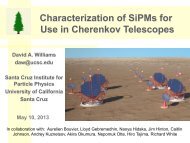
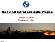
Homogeneous / isotropic / flat universe is a very unnatural stat 

Homogeneous / isotropic / flat universe is a very unnatural state 

for the universe. Problem of initial conditions Guth ’80 


Monday, June 21, 2010







Matter / radiation universe 

Faster (accelerated) expansion 

at t ≪ 1 s 

An accelerated expansion also 

Flattens the universe (explaining why Ωk,0 < 1%) 






Homogeneous / isotropic / flat universe is a very for the unnatural universe. state Problem of initial conditions 





at t ≪ 1 s 


Homogeneous / isotropic / flat universe is 

for Homogeneous the universe. / isotropic Problem/ flat of initial universe conditi is a v 


Big-bang cosmology 

Faster (accelerated) expansio 


at t ≪ 1 s 

at t ≪ 1 s 


Flattens the universe (explaining w 

Flattens the universe (explaining why 

Dilutes away unwanted relics ( 

Dilutes away unwanted relics (gr 







Homogeneous / isotropic / flat universe is a very for the unnatural universe. state Problem of initial conditions 




An accelerated expansion also An accelerated expansion also 

at t ≪ 1 s 

Homogeneous / isotropic / flat universe is 

for Homogeneous the universe. / isotropic Problem/ flat of initial universe conditi is a v 


Big-bang cosmology 

Faster (accelerated) expansio 

Homogeneous / isotropic / / flat flat universe is is a very a very unnatural state state 

for the universe. Problem Problemofof initial conditions conditionsGuth Guth ’80 ’80 



at t ≪ 1 s 

at t ≪ 1 s 



Flattens the universe (explaining w 

Flattens the universe (explaining why 

Dilutes away unwanted relics (gravitinos, monopoles,...) 

An accelerated expansion also Dilutes away unwanted relics ( 

Allows for large entropy (generated at reheating) 

Dilutes away unwanted relics (gr 



∼ 

6000 

180 

θ 

TT /2! [µK 2 ] 

5000 

4000 

ce: for any given k 

3000 

l(l+1)C l 

2000 

1000 illate in phase 

0 

10 50 

100 500 1000 

Multipole moment l 

. The 7-year temperature (TT) power spectrum from WMAP. The third acoustic peak and the onset of the Silk damping tail 

well measured by WMAP. The curve is the ΛCDM model best fit to the 7-year WMAP data: Ωbh2 = 0.02270, Ωch2 = 0.1107, 

38, τ= 0.086, ns= 0.969, ∆2 R = 2.38 × 10−9 , and ASZ= 0.52. The plotted errors include instrument noise, but not the small, 

d contribution due to beam and point source subtraction uncertainty. The gray band represents cosmic variance. A complete error 

t is incorporated in the WMAP likelihood code. The points are binned in progressively larger multipole bins with increasing l; 

anges are included in the 7-year data release. 

LSS 

. The high-l TT spectrum measured by WMAP, showing 

ovement with 7 years of data. The points with errors use 

ata set while the boxes show the 5-year results with the 

ning. The TT measurement is improved by >30% in the 

f the third acoustic peak (at l ≈ 800), while the 2 bins 

1000–1200 are new with the 7-year data analysis. 

(Most of the cosmological parameters reported 

paper were fit using a preliminary source correc- 

10 3 Aps = 11 ± 1 µK 2 sr. We have checked that 

ting the final result has a negligible effect on the 

ter fits.) After this source model is subtracted 

ch band, the spectra are combined to form our 

imate of the CMB signal, shown in Figure 1. 

-year power spectrum is cosmic variance limited, 

mic variance exceeds the instrument noise, up to 

. (This limit is slightly model dependent and can 

a few multipoles.) The spectrum has a signal- 

! 

, m ≡ orientation 

to-noise ratio greater than one per l-mode up to l = 919, 

and in band-powers of width ∆l = 10, the signal-to-noise 

ratio exceeds unity up to l = 1060. The largest improvement 

in the 7-year spectrum occurs at multipoles l > 600 

where the uncertainty is still dominated by instrument 

noise. The instrument noise level in the 7-year spectrum 

is 39% smaller than with the 5-year data, which makes it 

worthwhile to extend the WMAP spectrum estimate up 

to l = 1200 for the first time. See Figure 2 for a comparison 

of the 7-year error bars to the 5-year error bars. The 

third acoustic peak is now well measured and the onset 

of the Silk damping tail is also clearly seen by WMAP. 

As we show in §4, this leads to a better measurement 

of Ωmh 2 and the epoch of matter-radiation equality, zeq, 

which, in turn, leads to better constraints on the effective 

! 

T = 

WMAP 7 

 

∆TCMB with high coherence 

aℓm Yℓm ℓm 

T = 

number of relativistic species, Neff, and on the primor- 

dial helium abundance, YHe. The improved sensitivity 

at high l is also important for higher-resolution CMB 

experiments that use WMAP as a primary calibration 

source. 

2.4. Temperature-Polarization (TE, TB) Cross Spectra 

The 7-year temperature-polarization cross power spectra 

were formed using the same methodology as the 5year 

spectrum (Page et al. 2007; Nolta et al. 2009). For 

l ≤ 23 the cosmological model likelihood is estimated di- 

rectly from low-resolution temperature and polarization 

maps. The temperature input is a template-cleaned, coadded 

V+W band map, while the polarization input is a 

template-cleaned, co-added Ka+Q+V band map (Gold 

〈a ∗ ℓm aℓ ′ m ′〉 = C ℓ ∼ 

ℓ δℓℓ ′ δmm ′ 

1800 

ℓm, 

m ≡ orientation 

θ 

ℓ 

Coherence: for Cℓ ∝any 

given |aℓm| k2 

m=−ℓ 

all δ k oscillate in phase 

ax / min at same t) Acoustic peaks 


aℓm Yℓm 

(reach max ℓ ∼ / min at same t) Acoustic pe 

1800 


θ 

Acoustic peaks 

Peebles and Yu, ’70 Sunyaev, and Zel’dovich ’70 

Coherence: All δ k with the 

same k but = orientations

∼ 

6000 

180 

θ 

TT /2! [µK 2 ] 

5000 

4000 


3000 

l(l+1)C l 

2000 


0 

10 50 

100 500 1000 








LSS 


















! 










to l = 1200 for the first time. See Figure 2 for a compari- 

son of the 7-year error bars to the 5-year error bars. The 




of Ωmh2 and the epoch of matter-radiation equality, zeq, 


number of relativistic species, Neff, and on the primor- 

dial helium abundance, YHe. The improved sensitivity 



source. 





l ≤ 23 the cosmological model likelihood is estimated di- 

rectly from low-resolution temperature and polarization 

maps. The temperature input is a template-cleaned, coadded 

V+W band map, while the polarization input is a 


.5 Monday, June 21, 2010 

0 0.5 1 

! 

T = 

WMAP 7 

 



T = 

〈a ∗ ℓm aℓ ′ m ′〉 = Cℓ δℓℓ ′ 

ℓ ∼ 1800 

〈a 

, m ≡ orie 

θ 

∗ ℓm aℓ ′ m ′〉 = C ℓ ∼ 


1800 

ℓm, 

m ≡ orientation 

θ 

ℓ 

Coherence: for Cℓ ∝any 

given |aℓm| k2 

m=−ℓ 

all δk oscillate Acoustic in peaks phase 


aℓm Yℓm 

Peebles and Yu, ’70 Sunyaev, an 

(reach max / min at same t) Acoustic pe 


ℓ ∼ 1800 

θ 



same k but = orientations 

Peebles and Yu, ’70 Sunyaev, and Zel’dovich ’70 

must oscillate in phase 


same k but = orientations

∼ 

6000 

180 

θ 

TT /2! [µK 2 ] 

5000 

4000 


3000 

l(l+1)C l 

2000 


0 

10 50 

100 500 1000 








LSS 


















! 










to l = 1200 for the first time. See Figure 2 for a comparison 

of the 7-year error bars to the 5-year error bars. The 




of Ωmh2 and the epoch of matter-radiation equality, zeq, 


number! of relativistic species, Neff, and on the primordial 

helium abundance, YHe. The improved sensitivity 



source. 





l ≤ 23 the cosmological model likelihood is estimated directly 

from low-resolution temperature and polarization 

maps. The temperature input is a template-cleaned, co- 

added V+W band map, while the polarization input is a 


.5 Monday, June 21, 2010 

0 0.5 1 

WMAP 7 

〈a ∗ ℓm aℓ ′ m ′〉 = Cℓ δℓℓ ′ 

ℓ ∼ 1800 

T = 

, m ≡ orie 

θ 

 


〈a ∗ ℓm aℓ ′ m ′〉 = C ℓ ∼ 


1800 


T = 


θ 

Coherence: for any given k 

 

aℓm Yℓm 

ℓm 

ℓ 

Cℓ ∝ |aℓm| 2 

ℓm 

ℓ 

Cℓ ∝ |aℓm| 

m=−ℓ 

2 

ℓ ∼ 1800 

Cℓ ∝ |aℓm| 

m=−ℓ 


θ 

2 

ℓ ∼ 1800 


θ 


m=−ℓ 

all δk oscillate Acoustic in peaks phase 


Peebles and Yu, ’70 Sunyaev, an 

(reach max ℓ ∼ / min at same t) Acoustic pe 

Coherence: All δ with the 

k 1800 Coherence: All δk with the 


Coherence: θ All δk with the 



Acoustic Peebles, peaks Yu, ’70; Sunyaev, Zel’dovich ’7 

Peebles, Yu, ’70; Sunyaev, Zel’dovich ’70 

same kkbut but = = orientations 

Peebles and Yu, must ’70oscillate Sunyaev, inand phase Zel’dovich ’70 



No acoustic peaks if perturbation 

Coherence: All δk with the 

No acoustic peaks if perturbations 

actively sourced by defects 


actively sourced by defects

CMB gets polarized during scatterings; direct probe of what 

present on the LSS (ignore reionization) 


Hu and White ’97 


Net polarization in the direction 


from which fewer photons arrived 




CMB gets polarized on 


Any correlation at θ > 10 No appreciable perturbations expected at θ > 1 

is a cor 

scales on the LSS. Prediction 〈T E 

Coulson, Crittenden, Turok ’94 

0 No appreciable perturbations expected at θ > 1 

(the size of the 

horizon on the LSS) in models active models. If present, signal 

that “something” has caused super-horizon perturbations 



horizon on the LSS) in active models. If present, signal that 

“something” has caused super-horizon perturbations 

0 present on the LSS (ignore reionization) 









WMAP 

WMAP 7, 

stacked 

images 

of of of 

hot hot hot 

spots spots 

≡ ≡ horizon 

horizon today 

Spergel, Zaldarriaga ’97 


(• from ≡ horizon whichsize fewer at earlier photons times) Net arrived polarization in the 

(• ≡ horizon size at earlier times) 

Any correlation at θ > 10 Any correlation at θ > 1 is a correlation on super-horizon 

0 Any correlation at θ > 1 is a correlation on super-horizon 

0 is a correlation on super-horizon 

from which fewer photo 

scales scales on the LSS. Negligible signal from active models 

No appreciable correlation at θ > 10 No appreciable correlation at θ > 1 in defect models 

0 No appreciable correlation at θ > 1 in defect models 

0 in defect models 

for for which which no correlation on on super-horizon scales scales 

Coulson, Coulson, Crittenden, Turok Turok ’94 ’94 


Photons are reaching your eyes from it 


More γ 

— E < 0 E > 0 

Negative correlation on 

scales first acoustic peak 

WMAP Net polarization 

WMAP 7, stacked images in the 

of of direction 

hot hotspots spots 

atsu et al. 

Komatsu et al. 

WMAP 7, stacked images of hot spots 

WMAP 7, stacked images of hot Spergel, spots Zaldarriaga ’97 

WMAP SEVEN-YEAR OBSERVATIONS: POWER 

Active sources Seljak, Pen, Turok, 2.0 ’97 ℓ 

(• 1.5 

(• from ≡ ≡ horizon horizon which size fewer at earlier photons times) arrived 

scales on the LSS. Negligible signal from 0.0 active models 

-0.5 

No appreciable correlation at θ > 10 in defect models 

TE 2 

(l+1)Cl /2! [µK ] 

CMB gets polarized on 


Any correlation at θ > 10 No appreciable perturbations expected at θ > 1 

is a cor 

scales on the LSS. Prediction 〈T E 

Coulson, Crittenden, Turok ’94 



horizon on the LSS) in models active models. If present, signal 

that “something” has caused super-horizon perturbations 





0 present on the LSS (ignore reionization) 








≡ ≡ horizon 

horizon today 


Net polarization in the 


0 Any correlation at θ > 1 is a correlation on super-horizon 


1.0 

from which fewer photo 

scales on the LSS. Negligible signal from active models 

No appreciable correlation at θ > 10 No appreciable correlation at θ > 1in defect models 

0 in defect models 

for for which which no correlation on on super-horizon scales scales 

Coulson, Coulson, Crittenden, Turok Turok ’94 ’94 


0.5 

-1.0 

10 50 100 500 1000 


Figure 3. The 7-year temperature-polarization (TE) cross-power 

spectrum measured by WMAP. The second trough (TE

• Super-horizon correlations on the LSS 

• Inflation provides a causal mechanism for them 

• Alternative to inflation exist, but less complete 


• Super-horizon • Super-horizon correlations correlations on the on the LSS LSS 


Inflation 

• Inflation 

gives 

provides gives 

a causal 

a causal 

mechanism 

a causal mechanism 

for the 

mechanism for 

formation 

for thethem formation 

of perturbations leading to these correlations 

• Alternative of perturbations to inflation leading exist, to but these less correlations 

complete 

quantum fluctuations 


! 




d H 

Matter / Radiation 

Inflation 

! 

d 

H 

Matter / Radiation



Inflation 

• Inflation 

gives 


a causal 

a causal 

mechanism 


for the 

mechanism for 

formation 




complete 



! 




d H 


• Super-horizon correlations on the L 

Inflation 

• Inflation gives a causal mechanism for their form 


! 

• Alternative to inflation exist, but less com 

d 

H 

Matter / Radiation



Inflation 

• Inflation 

gives 


a causal 

a causal 

mechanism 


for the 

mechanism for 

formation 




complete 



! 



d H 



• Super-horizon correlations on the L 

Inflation 

• Inflation gives a causal mechanism for their form 


Inflation gives a causal mechanism for their formation 

• Alternative to inflation exist, but less com 



! 

d 

H 

Matter / Radiation

Slow 

Slow 

roll 

roll 

inflation 


Slow roll inflation 


Linde 

Linde 

’82 

’82 

Albrecht 

Albrecht 

and 

and 

Steinhradt 

Steinhradt 

’82 

’82 


Linde ’82 Albrecht and Steinh 

Linde ’82 Albrecht and Steinhradt ’82 

Scalar field slowly rolling due to Hubble friction 

Scalar Slowfield rollslowly inflation rolling due to Hubble friction 

ll inflation 

Potential energy slowly changes → a ≈ eH t 

Potential Linde ’82 energy Albrecht slowlyand changes Steinhradt → a ≈’82 eH t 

82 Albrecht and Steinhradt ’82 

Scalar field slowly rolling due to Hubble friction 

ld slowly rolling due to Hubble friction 

¨φ + 3 H ˙φ + dV 

¨φ + 3 H ˙φ + 

dφ dV 

H t 

dφ 

Potential energy slowly changes → a ≈ e 

l energy slowly changes → a ≈ e 

H t 

1/2 

= 0 1/2 

0 

, H ∝ V ¨φ + 3 H ˙φ + dV ¨φ + 3 H ˙φ + 1/2 

= 0 , H ∝ V 

dφ dV 

1/2 

= 0 , H ∝ V 

dφ 


Requires ɛ ≡ M 2 p 

2 

 

V ′ 2 

V 

≪ 1 , η ≡ M 2 p 

V ′′ 

V 

V 

≪ 1 

!

Requires ɛ ≡ M 2 p 

2 

 

V ′ 2 

V 

(Mp 10 GeV) 

≪ 1 , η ≡ M 2 p 

V ′′ 

V 

≪ 1 

1 

Pscalar = 

24 π2 M 4 V 

p ɛ | hor. cross. ∼ 5 · 10 −52 Ptensor = 2 

3 π2 V 

M 4 (Mp 10 

| hor. cross. unmeasured 

p 

• Small 

• Nearly scale invariant 

18 GeV) 

1 

Pscalar = 

24 π2 M 4 V 

p ɛ | hor. cross. ∼ 5 · 10 −52 Ptensor = 2 

3 π2 V 

M 4 • • Small 

• Small 

| hor. cross. unmeasured 

• Small Nearly scale invariant p 

• Nearly scale invariant • Nearly scale invariant 

• Nearly scale invariant 

• Suppressed tensor (to be rigorous, enhanced scalar) 

Ps ∝ k ns 

Ps ∝ k 

, ns 1 + 2η − 6ɛ 

ns , ns 1 + 2η − 6ɛ Ps ∝ k ns , ns 1 

Ps ∝ k ns−1 

, ns − 1 2η − 6ɛ 

• Suppressed tensor Enhanced (to bescalar rigorous, •power Suppressed enhanced tensor scalar) (to be rig 


• • Unknown scale scaleof of inflation ! (the ! • (the Unknown smaller smaller scale the scale, of inflation 

• 

the 

Unknown 

scale, 

scale of inflation ! (the smaller the scale, 

the flatter V ) 



• the Suppressed flatter V tensors ) (actually, enhanced • Suppressed scalars) tensors (actuall 


V 

!

Pscalar = 

1 

24 π2 M 4 p 

Ptensor = 2 

3 π2 V 

Ps ∝ k , ns 1 + 2η − 6ɛ 

M 4 p 

V 

ɛ | hor. cross. 

| hor. cross. 

∼ 5 · 10 −5 2 


ɛ ≡ 

V ′ 

unmeasured 

• Unknown scale of inflation ! Need to detect tensors 

• Suppressed tensors (actually, enhanced scalars) 

mall 

early scale invariant 

uppressed tensor V(to be rigorous, enhanced scalar) 

1/4 = 10 16 r ≡ Pt/Ps 

Larger r → larger V →• Larger larger ɛr → lar Infl 

• Scale of inflation from tensors (GW). Scalar > Tensor 

 

r 

 

r ≡ Pt/Ps 

1/4 

• Larger r → larger ɛ → Inflaton GeV moves more 

∆φ 

• Suppressed tensors (actually, 0.01 enhanced sc 

• Larger r → larger ɛ → Inflaton moves more 

Enhanced scalar power 

∆φ > ∼ Mp 

Large field models 

∆φ > ∼ Mp 


r 

V 

2 

V 1/4 = 10 16 GeV 

Measure GW, know V 


0.01 

r 

0.01 

1/2 

1/2 

≪ 1 

r 

0.01 

ɛ ∝ 

V ′ 

r ≡ Pt/Ps 

Lyth ’96 

1/4 

V 

2 

0.01 

≪ 1 

• Scale of inflation from tensors (GW). Scala 

• Suppressed tensors (actually, e 

Large field mod 

Measure GW, kn 

Small field mode

Pscalar = 

1 

24 π2 M 4 p 

Ptensor = 2 

3 π2 V 

Ps ∝ k , ns 1 + 2η − 6ɛ 

M 4 p 

V 

ɛ | hor. cross. 

| hor. cross. 

∼ 5 · 10 −5 2 


ɛ ≡ 

V ′ 

unmeasured 

r ≡ Pt/Ps 



V 

2 

≪ 1 

0.01 

mall 




1/4 = 10 16 r ≡ Pt/Ps 

Larger r → larger V →• Larger larger ɛr → lar Infl 

• Scale Larger • Larger of inflation r → larger from ɛ →ɛtensors Inflaton → Inflaton (GW). moves Scalar more moves > Tensor more 

 

r 

 

r ≡ Pt/Ps 

1/4 

• Larger r → larger ɛ → Inflaton GeV moves more 

• Suppressed tensors (actually, 0.01 enhanced∆φ sc 

r 1/2 

∆φ > 

• Larger r → larger∼ Mp ɛ → Inflaton 0.01 moves more 

r 1/2 

Lyth ’96 

Lyth ’96 

∆φ > ∼ Mp 

∆φ > 

∼ Mp 



∆φ > ∼ Mp 

r 


Large Measure field models GW, know V 

V 1/4 = 10 16 GeV 


r ≡ Pt/Ps 

0.01 

r 



r ≡ Pt/Ps 

0.01 

1/2 

1/2 

0.01 

r 

0.01 

ɛ ∝ 

V ′ 

1/4 

V 

2 

≪ 1 



Large field mod 


Small field mode

Pscalar = 

1 

24 π2 M 4 p 

Ptensor = 2 

3 π2 V 

Ps ∝ k , ns 1 + 2η − 6ɛ 

M 4 p 

V 

ɛ | hor. cross. • Larger r →ɛ ∝larger 

ɛ≪ →1 I 

• Suppressed tensor (to be rigorous, enhanced scalar) V 

ɛ ≡ 

| hor. cross. 

V ′ 

∼ 5 · 10 −5 2 

unmeasured 

r ≡ Pt/Ps 


V 

0.01 

• Larger r → larger ɛ → 

2 ≪ 1 


mall 




1/4 = 10 16 Larger r → larger V → larger ɛ → Infl 

• Scale of inflation from tensors (GW). Scalar > Tensor 

 

r 

1/4 GeV 

• Suppressed tensors (actually, 0.01 enhanced sc 

V 1/4 = 10 16 ∆φ > 

r ≡ Pt/Ps 

• Larger ∼ Mp 

r → lar 

• Larger • Larger r → larger ɛ →ɛInflaton → Inflaton moves more ∆φ > 0 

moves more ∼ Mp 

• Larger r → larger r ≡ Pt/Ps 

Lyth ’96 

ɛ → Inflaton moves more 

∆φ 

r 1/2 Large field models 

∆φ > 

• Larger r → larger∼ Mp ɛ → Inflaton moves Large field models 

0.01 more 

r 1/2 

∆φ > 

r 1/2 

Lyth ’96 

∆φ > ∼ Mp 

∼ Mp 0.01 Measure GW, know V 

Lyth ’96 

0.01 

 

r 1/2 r Large 1/4field 

mod 

∆φ > 

∼ Mp GeV 

Large 0.01 

Large 

Largefield field 

field 

models 

models 

Small field models 

models Small field 0.01models 


Large Measure field models GW, know V 




r ≡ Pt/Ps 

r ≡ Pt/Ps 

 


Bad luck ! 

Bad luck ! 

V ′ 

2 


 

Small field mode

Examples 

Examples Examplesof of of large 

large field 

field field models 

models 

Examples of large field models 


(Mathematically) simplest, single field / single scale models 


Chaotic inflation: 

V = 1 

2 m2 φ 2 , λ 

4 φ4 Chaotic inflation: 

, . . . 

V = 1 

2 m2 φ 2 , λ 

4 φ4 Chaotic inflation: 

, . . . 

V = 1 

2 m2 φ 2 , λ 

4 φ4 , . . . 

V = 1 


V = 1 

2 m2 φ 2 , λ 

4 φ4 Examples of large field models 


, . . . 


2 m2 φ 2 , λ 

4 φ4 , . . . 


Natural inflation: 

Natural inflation: V = 1 


V = V0 


 

1 − cos φ 

f 

2 

 

m2 φ 2 , λ 

4 φ4 , . . . 

V = V0 

V = V0 

V = V0 

1 − cos φ 

1 − cos f 

φ 

 

f 

Hill-top (symm. breaking): 

Hill-top (symm. breaking): 

pφ V = V0 1 −φ 

V = V0 1 − f 


 

1 − cos φ 

f 

f 

p 

+ . . . 

 

+ . . .

Examples of small field models 



Hybrid Examples inflation: of large field models 

Hybrid inflation: 


id inflation: 

 

σ 2 − v 22 g 

+ 2 

2 φ2 σ 2 



V = λ 

4 

V = λ 

σ 

4 

2 − v 22 g 

+ 2 

2 φ2 σ 2 

V = λ 

σ 

4 

2 − v 22 g 

+ 2 

2 φ2 σ 2 


V = 1 

2 m2 φ 2 , λ 

4 φ4 V = Supergravity: , . . . 

λ 

σ 

4 

2 − v 22 g 

+ 2 

2 φ2 σ 2 

V = λ 

σ 

4 

2 − v 22 g 

+ 2 

2 φ2 σ 2 



Natural inflation: 4 

 

 

φ4 Realized in supergravity (no large 

, . . . 

exp K = exp ∂φi 

φ2 

M 2 Realized in supergravity (no large exp K = exp 

terms) 

p 

and in D−brane inflation (string theory) 

φ2 

M 2 terms) 

p 

and in D−brane inflation (string theory) 


Supergravity: 

V = 1 

2 m2 φ 2 , λ 

Supergravity: V = V0 

V = V0 

 



1 − cos φ 

f 

V = λ 

σ 

4 

2 − v 22 g 

+ 2 

2 φ2 σ 2 

K = φi φ ∗ i ⇒ V = VD+VF , VF = e K 

M 2 p 

∂W 

1 − cos φ 

K 

M 

e f2 

p 1 for φ ≪ Mp , Vhybrid typical VD+VF ! 

+ φ ∗ 

 

i W 

 

2 

− 

" 

 

3|W |2 



p 

p 

K = φi φ φ φ 

V = V0 V = 1 −V0 

1 −+ 

. . . + . . f. ≪ Mp 

f f 

∗ i ⇒ V = VD+VF , VF = e K 

M2 ∂W 

p + φ 

∂φi 

∗ 

2 

i W 

3|W |2 

− 

M 2 

K = φi φ 

p 

∗ i ⇒ V = VD+VF , VF = e K 

M2 ∂W 

p + φ 

∂φi 

∗ 

2 

i W 

3|W | 

− 

M 2 p 


M 2 p

−2.7 

σ8 0.801 ± 0.030 0.796 ± 0.036 

Ωb 0.0449 ± 0.0028 0.0441 ± 0.0030 

Ωc 0.222 ± 0.026 0.214 ± 0.027 

3196 +134 

3176 +151 

Where we stand 

zeq 

−133 

WMAP 7 

−150 

zreion 10.5 ± 1.2 11.0 ± 1.4 

a Models fit to WMAP data only. See Komatsu et al. (2010) 

for additional constraints. 

WMAP only 

WMAP7 + ACBAR + QUaD: ns = 0.979±0.018 , r < 0.33 (95% CL) 

WMAP only 

WMAP7 + ACBAR + QUaD: ns = 0.979±0.0 

WMAP7 + BAO + H0 : ns = 0.973±0.014 , r < 0.24 (95% CL) 

WMAP7 + BAO + H0 : ns = 0.973±0.0 

e 10. Gravitational wave constraints from the 7-year WMAP data, expressed in terms of the tens 

rs show the 68% and 95% confidence regions for r compared to each of the 6 ΛCDM parameters us 

rs are 

WMAP7 WMAP the corresponding 

+ ACBAR 7 5-year results. We do not detect gravitational waves with the new data; w 

parameters the 7-year limit is + r QUaD: < 0.36 (95% ns CL), = 0.979±0.018 compared to the 5-year , r < limit 0.33 of(95% r < 0.43 CL) (95% C 

P data are combined with H0 and BAO constraints (Komatsu et al. 2010). 

n etWMAP7 al. 2006; Komatsu + BAO + etH0 al. : 2009). ns = The 0.973±0.014 relative , the r < curvaton 0.24 (95% model. CL) For the 

itude of its power spectrum is parameterized by α, vention in which anticorrelati 

WMAP7 + BAO + H0 : ns = 0.973±0.014 low, multipoles r < 0.24 (95% (Komatsu CL) et al 

α PS(k0) 


≡ , (14) The constraints on both typ 

constraints from the 7-year WMAP data, expressed in terms of the tensor-to-scalar ratio, r. The red

Quest for r 

v = ∇φ + ∇ × A = electric + magnetic 

v = ∇φ + ∇ × A = elec 


Scalar perturbations 

Tensor perturbations 

E−mode polarization 

B−mode polarization 

WMAP 5 

r < 0.36 WMAP7, r < 0.33 WMAP7 

r < 0.24 WMAP7 + BAO + H0, r

v = ∇φ + ∇ × v = A = electric + magnetic 

∇φ + ∇ × A = electric + magnetic Tensor perturbations 

v = ∇φ + ∇ × A = elec 






Quest for rScalar 

perturbations 

Scalar perturbations E−mode polarization 





WMAP 5 

r < 0.36 WMAP7, r < 0.33 WMAP7 

r < 0.24 WMAP7 + BAO + H0, r


∇φ + ∇ × v = 

A = electric + magnetic Tensor perturbations 




v = 



∇φ + ∇ × A = elec 











perturbations 






WMAP 5 

r < 0.36 WMAP7, r < 0.33 WMAP7 

r < 0.24 WMAP7 + BAO + H0, r


∇φ + ∇ × v = 

A = electric + magnetic Tensor perturbations 




v = 



∇φ + ∇ × A = elec 










perturbations 

v = ∇φ + ∇ × A = elec 





12 Komatsu et al. 



WMAP 5 




WMAP 5 

r < 0.36 WMAP7, r < 0.33 WMAP7 

r < 0.24 WMAP7 + BAO + H0, r < 

Fig. 2.— How the WMAP temperature and polarization data constrain the tensor-to-scalar ratio, r. (Left) The con 

95% CL. The gray region is derived from the low-l polarization data (TE/EE/BB at l ≤ 23) only, the red region from t 


plus the high-l TE data at l ≤ 450, and the blue region from the low-l polarization, the high-l TE, and the low-l

Planck (bluebook) 



• Launched 

Launched 5/2009 

5/2009 

• Launched 5/2009 


•Planck • 

First 

First sky 

sky 

survey 

survey 

1/2010 

1/2010 

• First sky survey 1/2010 


• Second 

Second sky 

sky 

survey 

survey 

7/2010 

7/2010 

•Launched Second sky survey 5/2009 7/2010 

• Second sky survey 7/2010 First sky survey 1/2010 

•Second • First-year sky release survey 7/2012 7/2010 Release first-year 

• First-year release 7/2012 


res. 7/2012 

DT 

DT DT cosmic-variance cosmic-variance 

l l 

2000 2000 

for for for 

polarization: 

polarization: 

DT small cosmic-variance l 2000 for polarization: 

small scales 

only only 

slight slight 

help help 

with with 

parameters, 

parameters, 

but allows important consistency cross-check 

but (lessallows important consistency cross-check 

(less SZ 

in in 

EE) 

(less SZ in EE) 

small but PLOT allows scales SPECTRA important only slightconsistency helpFROM with parameters, cross-check BLUE BOOK 

DT cosmic-variance l 2000 for polarization: 

r 0.1 

0.1 in 

14 

months 

r r 

0.05 

in in 

28 28 

months 

r 0.1 in 14 months r 0.05 in 28 months 

(Efstathiou, (Efstathiou, small (Efstathiou, scales Gratton only 09) slight help with parameters, 

(Efstathiou, Gratton 09) 







• Launched 


5/2009 


• •Launched Launched 5/2009 

•Planck • 

First 

First sky 

sky 

survey 

survey 

1/2010 

1/2010 


• •First First sky skysurvey survey 1/2010 

• Second 

Second sky 

sky 

survey 

survey 

7/2010 

7/2010 

• Second sky survey 7/2010 

2.3 Cosmological Parameters from Planck 33 

0 


10 50 





the bin ranges are included in the 7-year data release. 


res. 7/2012 


DT 


l l 

2000 2000 

for for for 

polarization: 

polarization: 

TT DT small cosmic-variance l 2000 for polarization: 

small scales 

only only 

slight slight limited 

help help ℓ < 

∼ 

with with 2000 

parameters, 

parameters, 


for but polarization: allows important small scales consistency only slight 

(less cross-check help 

(less SZ 

in in 

EE) 

with (lessparameters, SZ in EE) but allows important consistency 

cross-check (less SZ in EE) 


(small anisotropy 

For simplicity, take unive 

WMAP 5 years ( 

100 500 1000 

Groeneboom and Erikse 

Planck 2012 

mask. (Most of the cosmological parameters reported 


in this paper were fit using a preliminary source correc- 

r 0.1 

0.1 in 

14 

months 

r r 

0.05 

in in 

28 28 

months 

tion of 10 





and angular resolution of Planck. 


3Aps = 11 ± 1 µK2 sr. We have checked that 

substituting the final result has a negligible effect on the 

parameter fits.) After this source model is subtracted 

from each band, the spectra are combined to form our 

best estimate of the CMB signal, shown in Figure 1. 

The 7-year power spectrum is cosmic variance limited, 

i.e., cosmic variance exceeds the instrument noise, up to 

l = 548. (This limit is slightly model dependent and can 

vary by a few multipoles.) The spectrum has a signal- 

TT 2 

l(l+1)Cl /2! [µK ] 

FIG 2.8.—The left panel shows a realisation of the CMB power spectrum of the concordance ΛCDM model (red 

line) after 4 years of WMAP observations. The right panel shows the same realisation observed with the sensitivity 

since the fluctuations could not, according to this naive argument, have been in causal contact 

6000 

5000 

4000 

3000 

2000 

1000 

Figure 1. The 7-year temperature (TT) power spectrum from WMAP. The third acoustic peak and the onset of the Silk dam 

are now well measured by WMAP. The curve is the ΛCDM model best fit to the 7-year WMAP data: Ωbh2 = 0.02270, Ωch2 ΩΛ= 0.738, τ= 0.086, ns= 0.969, ∆2 R = 2.38 × 10−9 , and ASZ= 0.52. The plotted errors include instrument noise, but not 

correlated contribution due to beam and point source subtraction uncertainty. The gray band represents cosmic variance. A comp 

treatment is incorporated in the WMAP likelihood code. The points are binned in progressively larger multipole bins with inc 

Figure 2. The high-l TT spectrum measured by WMAP, showing 

the improvement with 7 years of data. The points with errors use 

the full data set while the boxes show the 5-year results with the 

same binning. The TT measurement is improved by >30% in the 

vicinity of the third acoustic peak (at l ≈ 800), while the 2 bins 

from l = 1000–1200 are new with the 7-year data analysis. 




WMAP 2010 Pla 

to-noise ratio greater than one per l-mode up to 

and in band-powers of width ∆l = 10, the signal 

ratio exceeds unity up to l = 1060. The largest 

ment in the 7-year spectrum occurs at multipoles 

where the uncertainty is still dominated by ins 

noise. The instrument noise level in the 7-year s 

is 39% smaller than with the 5-year data, which 

worthwhile to extend the WMAP spectrum esti 

to l = 1200 for the first time. See Figure 2 for a c 

son of the 7-year error bars to the 5-year error b 

third acoustic peak is now well measured and t 

of the Silk damping tail is also clearly seen by 

As we show in §4, this leads to a better meas 

of Ωmh 2 and the epoch of matter-radiation equa 

which, in turn, leads to better constraints on the 

number of relativistic species, Neff, and on the 

dial helium abundance, YHe. The improved se 

at high l is also important for higher-resolutio 

experiments that use WMAP as a primary ca 

source. 

2.4. Temperature-Polarization (TE, TB) Cross 

The 7-year temperature-polarization cross pow 

tra were formed using the same methodology a 

year spectrum (Page et al. 2007; Nolta et al. 20 

l ≤ 23 the cosmological model likelihood is estim 

rectly from low-resolution temperature and pola 

maps. The temperature input is a template-clea 

added V+W band map, while the polarization in 

template-cleaned, co-added Ka+Q+V band ma



6000 


•• • 

Launched 


5/2009 

5000 



4000 

• •Launched Launched 5/2009 

3000 

• •Planck First 

•First First sky 

Firstsky sky 

skysurvey survey survey1/2010 1/2010 

1/2010 

2000 


• •First First sky skysurvey survey 1/2010 

1000 

• •Second •Second Second sky 

Second sky skysurvey survey survey7/2010 7/2010 

7/2010 

• Second sky survey 7/2010 




TT DTcosmic-variance DT DT cosmic-variance cosmic-variance cosmic-variancelimited l l 

2000 2000 2000ℓ < 

TT cosmic-variance limited 

∼ 

for for for 2000 

ℓ < 

polarization: 

polarization: 

TT DT small cosmic-variance l 2000 for polarization: 

small scales 

only only 

slight slight limited 

help help ℓ < 

∼ 

with with 2000 ∼ 2000 

parameters, 

parameters, 

EE and TE c.v. lim. ℓ < 

but allows important consistency ∼ 1000 

cross-check 

for EE 

but polarization: and TE c.v. 

(lessallows important small lim. scales ℓ < 

consistency ∼ 1000 only slight cross-check help 

(less SZ 

in in 

EE) 

with 

(less parameters, 

SZ in EE) 

but allows important consistency 

(less SZcross-check in EE) (less SZ in EE) 


0 


10 50 







res. 7/2012 





100 500 1000 


Planck 2012 




r 0.1 

0.1 in 

14 

months 

r r 

0.05 

in in 

28 28 

months 








3Aps = 11 ± 1 µK2 sr. We have checked that 



from each band, the spectra are combined to form our 

best estimate of the CMB signal, shown in Figure 1. 

The 7-year power spectrum is cosmic variance limited, 

i.e., cosmic variance exceeds the instrument noise, up to 

l = 548. (This limit is slightly model dependent and can 

vary by a few multipoles.) The spectrum has a signal- 

TT 2 

l(l+1)Cl /2! [µK ] 











for polarization: small scales only slight help 


with parameters, but allows important con- 


sistency cross-check (less SZ in EE) 

for polarization: small scales only slight help 

with parameters, but allows important consistency 

cross-check (less SZ in EE) 


WMAP 2010 Pla 




















source. 









template-cleaned, co-added Ka+Q+V band ma 



since the fluctuations could not, according to this naive argument, have been in causal contact



6000 


• Launched 


5/2009 

5000 


4000 


3000 

•Planck • 

First 

First sky 

sky 

survey 

survey 

1/2010 

1/2010 

2000 



1000 

• Second 

Second sky 

sky 

survey 

survey 

7/2010 

7/2010 

0 

• Launched Second sky survey 

Second sky survey 5/2009 7/2010 

10 50 

7/2010 First sky survey 1/2010 






res. 7/2012 

DT 


l l 

2000 2000 

for for for 

polarization: 

polarization: 

DT small cosmic-variance l 2000 for polarization: 

small scales 

only only 

slight slight 

help help 

with with 

parameters, 

parameters, 

small but PLOT scales SPECTRA only slight helpFROM with parameters, BLUE BOOK 

but allows 

important 

consistency 

cross-check 

but (lessallows important consistency cross-check 

(less SZ 

in in 

EE) 











r 0.1 

0.1 in 

14 

months 

r r 

0.05 

in in 

28 28 

months 








3Aps = 11 ± 1 µK2 • Launched 5/2009 

09 

/2010 


• •Launched Launched Second sky 5/2009 

survey• First 7/2010 sky survey 1/2010 

1/2010 

y 7/2010 

• Launched 5/2009 • Second sky survey 7/2010 

vey• • 7/2010 

•First First First-year sky survey release 1/2010 

7/2012 

7/2012 • First sky survey 1/2010 • First-year release 7/2012 

se • 7/2012 TT Second cosmic-variance sky 

sky 

survey 

survey 

7/2010 

7/2010 

limited ℓ < 

∼ 2000 

e limited • Secondℓ < 

∼sky 2000 survey 7/2010 TT cosmic-variance limited ℓ < 

∼ 2000 

nce• limited EE First-year andℓ < 

• First-year ∼TE 2000 release c.v. lim. 7/2012 ℓ < 

release 7/2012 ∼ 1000 

. •ℓ First-year < 

∼ 1000 release 7/2012 EE and TE c.v. lim. ℓ < 

∼ 1000 

lim. TT (less ℓ < 

∼cosmic-variance 1000 SZ in EE) limited ℓ < 

TT cosmic-variance limited 

∼ 2000 

(less SZ ℓ < 

TT cosmic-variance limited ℓ < in 

∼ 2000 ∼EE) 2000 

EE forand polarization: TE c.v. lim. small ℓ < 

∼ 1000 

for EEpolarization: and TE c.v. small lim. for 

scales ℓ < polarization: scales only 

∼ 1000 small slight scales helponly 

slight help 

with parameters, but allows 

only slight 

important 

help 

con- 

small 

all scales 

withscales only 

parameters, only 

slight 

slight 

help with parameters, but allows important con- 


but help allows important con- 

ut sistency cross-check (less SZ in EE) 

but allows 

sistency (less allowsimportant SZcross-check important consistency cross-check (less SZ in EE) 

in EE) (less con- SZ in EE) 

keck (less (lessSZ SZinin EE) 

sr. We have checked that 



for r > polarization: smallr scales 

> 

only from each slight band, the spectra help are combined to form our 

r 0.1 ∼ 0.1 in 14 months∼ 0.1 

r > in 14 months r > 

in 14 months r 0.05 ∼ 0.05 in 28 months ∼ 0.05 in 28 months 

in 28 best estimate months 

of the CMB signal, shown in Figure 1. 

for polarization: small scales only The 7-year power slight spectrum is cosmic help variance limited, 

with parameters, but allows important i.e., cosmic variance exceeds con- the instrument noise, up to 

nths s l = 548. (This limit is slightly model dependent and can 

(Efstathiou, r > r > 

∼ 0.05 inGratton 28 months 09) 

vary by a few multipoles.) The spectrum has a signalsistency 

with 

∼ 0.05 in 28 months 

Efstathiou, 

parameters, cross-check Gratton 

butEfstathiou, (less 09 

allows SZ inimportant Gratton 09 

EE) con- 

Monday, sistency June 21, 2010cross-check 


TT 2 

l(l+1)Cl /2! [µK ] 

WMAP 2010 Pla 





100 500 1000 






Planck 2012 




















source. 









template-cleaned, co-added Ka+Q+V band ma 



since the fluctuations could not, according to this naive argument, have been in causal contact

Ω c h 2 

n run 

τ 

n s 

log[10 10 A s ] 

H 0 

0.12 

0.0210.0230.025 

0.1 

0.15 

0.1 

0.05 

0.0210.0230.025 

0.0210.0230.025 

1.1 

1.1 

1 

0.9 

0.05 

0.0210.0230.025 

0 

−0.05 −0.05 

0.0210.0230.025 

3.2 

3.2 

3.1 

3 

0.0210.0230.025 

0.15 

0.1 

0.05 

1 

0.9 

0.05 

0 

3.1 

3 

Ω h 

b 2 

85 

85 

80 

80 

75 

75 

70 

70 

65 

65 

0.0210.0230.025 

0.1 0.12 

0.1 0.12 0.05 0.1 0.15 

1.1 

0.1 0.12 

0.9 1 1.1 

−0.05 −0.05 

0.1 0.12 0.05 0.1 0.15 0.9 1 1.1−0.05 

0 0.05 

3.2 

3.2 

3.2 

0.1 0.12 

Ω h 

c 2 

0.1 0.12 

1 

0.9 

0.05 

0 

3.1 

3 

0.05 0.1 0.15 

0.05 0.1 0.15 

0.05 

0 

3.1 

3 

0.9 1 1.1−0.05 

0 0.05 

85 

85 

85 

80 

80 

80 

75 

75 

75 

70 

70 

70 

65 

65 

65 

0.05 0.1 0.15 

τ 

0.9 1 1.1−0.05 

0 0.05 

n s 

3.1 

3 

Efstathiou, Gratton 09 

WMAP4 vs. Planck1 

n run 

85 

80 

75 

70 

65 

3 3.1 3.2 

3 3.1 3.2 

log[10 10 A s ] 

65 75 85 

H 0 

Monday, 

FIG 2.18.—Forecasts June 21, 2010 

of 1 and 2σ contour regions for various cosmological parameters when the spectral index

Non-gaussianity 

R ∼ 10−5 single field slow roll inflation (potential Models extremely with flat) mu 


flation, 

Noninteracting inflaton → gaussianity. At Models least with gravity. multiple Tiny fields (∼ 10(many fie 

⇒ fNL ∼ 10 means nongaussianity at 0.01% level 

flation, 

Salopek, Bond ’9 

Komatsu, Spergel Salopek, ’00 Bond ’90 Maldacena ’02 

Gaussian prediction forMaldacena nonintercting ’02 inflaton All models at least 

−6 ) 

non-gaussianity for single field slow roll inflation (flat potential) 

R ∼ 10−5 Noninteracting inflaton → gaussianity. At least gravity. Tiny (∼ 10 


−6 ) 


R ∼ 10−5 ⇒ fNL ∼ 10 means nongaussianity at 0.01% level 



gravitational interaction. Nongaussianity is small (fNL∼0.05) for 

Komatsu, Spergel ’00 


single field slow roll inflation (potential extremely flat) 

Gaussian prediction for nonintercting inflaton All models at least 



Models with multiple fields (multiple fields inflation, curvaton, 

modulated perturbations) have isocurvature → curvature pertur- 



bations conversion outside horizon, where gradients are irrele- 

vant. Predicted nongaussianity of the local type. 



Inflaton with nonstandard kinetic term: k − 


Models 

modulated 

with 

perturbations) 

multiple fields 

have 

(multiple 

isocurvature 

fields 

→ 

inflation, 

curvature 

curvaton, 

pertur- 

modulated 

bations conversion 


outside 

have 

horizon, 

isocurvature 

where gradients 

→ curvature 

are 

perturirrele- 

bationsvant. Predicted conversion nongaussianity outside horizon, of thewhere local type. gradients are irrele- 


vant. Predicted nongaussianity of the local type.





flation, 



flation, 



Gaussian prediction forMaldacena nonintercting ’02 inflaton All models at least 





−6 ) 


R ∼ 10−5 Noninteracting inflaton → gaussianity. At least gravity. Tiny (∼ 10 




−6 ) 


R ∼ 10−5 ⇒ fNL ∼ 10 means nongaussianity R ∼at 10 0.01% level 




−5 Non-gaussianity 

aussianity for single field slow roll inflation (flat potential) 

〈 Rk1 

Rk2 

Rk3 〉 = (2π) 

⇒ fNL ∼ 10 means nongaussian 


3 δ (3) (k1 + k2 + k3) BR (k1, k2, k3) 

Phenomenological parametrization 

R ∼ 10−5 non-gaussianity for single field slow roll inflation (flat potential) 

〈 Rk1 

Rk2 

Rk3 〉 = (2π) 







3 δ (3) (k1 + k2 + k3) BR (k1, k2, k3) 


R (x) = Rg (x)+ 3 

local 

fNL Rg (x) 

5 2 − 〈Rg (x) 2 〉 


R ∼ 10−5 Phenomenological parametrization 

R (x) = Rg (x)+ 



3 

local 

fNL Rg (x) 

5 2 − 〈Rg (x) 2 〉 


Since local in space, called local non-gaussianity 

R ∼ 10−5 R (x) = Rg (x)+ 


3 

local 

fNL Rg (x) 

5 2 − 〈Rg (x) 2 〉 



( since R ∼ 10−5 , ⇒ fNL ∼ 10 means nongaussianity at 0.01% level ) 

nteracting inflaton → gaussianity. At least gravity. Tiny (∼ 10 −6 ) 


modulated Gaussian prediction perturbations) for nonintercting have isocurvature inflaton → curvature All models pertur- at least 


bationssingle conversion single field slow outside field roll inflation horizon, slow(potential where roll inflation extremely gradientsflat) (potential extremely flat) 

gravitational Gaussian interaction. prediction Nongaussianity for nonintercting is small (fNL∼0.05) 

are irrele- for inflaton All models at least 

vant. Predicted single nongaussianity field slow of the vant. roll localPredicted inflation type. nongaussianity (potential extremely of the local flat) type. 

single Models field with multiple fields (multiple fields inflation, curvaton, 

gravitational slow roll inflation interaction. (potential extremely Nongaussianity flat) 

is small (fNL∼0.05) for 




bations single conversion fieldoutside slowhorizon, roll inflation where gradients (potential are irrele- extremely flat) 

inflationModels 

modulated 

with 



have 

(multiple 

isocurvature 

fields 

→ 


curvature 

curvaton, 


pertur- 




Salopek, modulated 

bations Bond ’90 conversion 


outside 

have 

horizon, 

isocurvature 


→ curvature 

are 

perturirrele- 

Maldacena bationsvant. ’02Predicted 

conversion nongaussianity outside horizon, of thewhere local type. gradients are irrele- 








flation, 



flation, 


−6 Noninteracting inflaton → gaussianity. At least gravity. Tiny (∼ 10 

) 


nteracting inflaton → gaussianity. At least gravity. Tiny (∼ 10 

) 

−6 ) 


〈 Rk1 

Rk2 

Rk3 〉 = (2π) 3 δ (3) non-gaussianity for single field slow roll inflation (flat potential) 

〈 Rk1 

Rk2 

Rk3 〉 = (2π) 

(k1 + k2 + k3) BR (k1, k2, k3) 

3 δ (3) Phenomenological parametrization 

(k1 + k2 + k3) BR (k1, k2, k3) 

R (x) = Rg (x)+ 3 

local 

f Rg (x) 2 − 〈Rg (x) 2 〉 


R (x) = Rg (x)+ 


3 

f 

local 

NL Rg (x) 

5 2 



R ∼ 10−5 R (x) = Rg (x)+ ⇒ fNL ∼ 10 means nongaussian 

3 


Since local in space, called local no 


R ∼ 10 Gaussian prediction forMaldacena nonintercting ’02 inflaton All models at least 



−5 R ∼ 10 



−5 Phenomenological ⇒parametrization fNL ∼ 10 means nongaussianity at 0.01% level 

R ∼ 10 



−5 Phenomenological parametrization 


R (x) = Rg (x)+ 



3 

local 

fNL Rg (x) 

5 2 − 〈Rg (x) 2 〉 

R (x) = Rg (x)+ 


3 

local 

fNL Rg (x) 

5 2 − 〈Rg (x) 2 〉 

 

local 

fNL Rg (x) 

Komatsu, 5 Spergel ’00 



2 − 〈Rg (x) 2 〉 

〈 Rk1 

Rk2 

Rk3 〉 = (2π) 3 δ (3) (k1 + k2 + k3) 




single field 

R ∼ 10 

slow roll inflation (potential extremely flat) 



−5 Since local in space, called local non-gaussianity 


R ∼ 10−5 ( since R⇒ fNL ∼ 10 ∼ 10 means nongaussianity at 0.01% level 


, ⇒ fNL ∼ 10 means nongaussianity at 0.01% level ) 


RModels ∼ 10Gaussian with multiple prediction fields for nonintercting (multiple modulated fields inflaton inflation, All perturbations) models curvaton, at least have isocurvature → curvature pertur- 

−5 , ⇒ fNL ∼ 10 means nongaussianity at 0.01% level ) 

modulated Gaussian gravitational prediction perturbations) interaction. for nonintercting have Nongaussianity isocurvature inflaton →is curvature small All models (fNL∼0.05) pertur- at least for 

5 

NL 


bations conversion outside horizon, where gradients are irrelebationssingle 

conversion single field slow outside field roll inflation horizon, slow(potential where roll inflation extremely gradientsflat) are(potential irrele- extremely flat) 

gravitational Gaussian interaction. prediction Nongaussianity for nonintercting is small (fNL∼0.05) for inflaton All models at least 

〈 Rk1 

Rk2 

Rk3 〉 = (2π) vant. Predicted nongaussianity of the local type. 

3 δ (3) 

 

(k1 + k2 + k3) BR (k1, k2, k3) T (x) T (y) T (z) 

vant. Predicted single nongaussianity field slow of theroll local inflation type. 

single Models field with multiple fields (multiple fields inflation, curvaton, (potential extremely flat) 






bations single conversion fieldoutside slowhorizon, roll inflation where gradients (potential are irrele- extremely flat) 


modulated 

with 



have 

(multiple 

isocurvature 

fields 

→ 


curvature 

curvaton, 

From vant. *, and Predicted from nongaussianity scale invariant of the local type. power spectrum, 

pertur- 






outside 

have 

horizon, 

isocurvature 


→ curvature 

are 

perturirrele- 








( since R ∼ 10 −5 , ⇒ fNL ∼ 10 means nongaussianity at 







flation, 



flation, 


Salopek, Bond ’90 Maldacena ’02 


) 




) 


−6 ) 


〈 Rk1 

Rk2 


〈 Rk1 

Rk2 

Rk3 〉 = (2π) 

(k1 + k2 + k3) BR (k1, k2, k3) 


(k1 + k2 + k3) BR (k1, k2, k3) 

R (x) = Rg (x)+ 3 

local 

fNL Rg (x) 

5 2 − 〈Rg (x) 2 〉 


R (x) = Rg (x)+ 


3 

f 

local 

NL Rg (x) 

5 2 

Since local in space, called local non-gaussianit 




R 

Phenomenological 

(x) = Rg (x)+ ⇒parametrization fNL ∼ 10 means nongaussianity at 0.01% level 

3 

local 

fNL Rg (x) 

5 2 − 〈Rg (x) 2 〉 

R (x) = Rg (x)+ 3 

local 

fNL Rg (x) 

5 2 − 〈Rg (x) 2 〉 

e R ∼ 10−5 , ⇒ fNL ∼ 10 means nongaussianity at 0.01% level ) 

R ∼ 10−5 R ∼ 10 


−5 Since local in⇒ space, fNL ∼ 10called means nongaussian local no 



gravitational interaction. Nongaussianity Komatsu, is Spergel small (fNL∼0.05) ’00 for 




−5 ⇒ fNL ∼ 10 means nongaussianity at 0.01% level 

R (x) = Rg (x)+ 



3 

local 

fNL Rg (x) 

5 2 − 〈Rg (x) 2 〉 


Komatsu, SinceSpergel local’00 in space, called local 〈 non-gaussianity 

Rk1 

Rk2 

Rk3 〉 = (2π) 3 δ (3) From *, and from scale invariant power spectrum, 


(k1 + k2 + k3) 




single field 

R ∼ 10 








, ⇒ fNL ∼ 10 means nongaussianity at 0.01% level ) 


RModels ∼ 10Gaussian with multiple prediction fields for nonintercting (multiple modulated fields inflaton inflation, All perturbations) models curvaton, at least have isocurvature → curvature pertur- 

−5 , ⇒ fNL ∼ 10 means nongaussianity at shape 0.01% level ) 



bations conversion outside horizon, where gradients are irrelebationssingle 



〈 Rk1 

Rk2 

Rk3 〉 = (2π) vant. Predicted nongaussianity of the local type. 

3 δ (3) From *, and from scale invariant power spectrum, 

 

 










single field slow roll inflation (potential extremely 

1 

flat) 



modulated 

with 


multiple Inflatonfields with have 

(multiple nonstandard BR ∝ 

isocurvature 

fields 

→ 

inflation, + kinetic curvature 

curvaton, 

From vant. *, and Predicted from nongaussianity scale invariant of the local type. power spectrum, (k1 k2) 

3 term: pertur- k − 


1 

+ 

(k1 k2) 

3 1 

(k1 k2) 3 

From *, and from scale invariance 




outside 

have 

horizon, 

isocurvature 


→ curvature 

are 

perturirrele- 










shape 

B ∝ 


1 + 1 + 1 

Models with multiple fields (multiple fields inflation, curvaton 

modulated perturbations) have isocurvature → curvature pertur 

bations conversion outside horizon, where gradients are irrele 








flation, 



flation, 


Salopek, Bond ’90 Maldacena ’02 


) 




) 


−6 ) 


〈 Rk1 

Rk2 


〈 Rk1 

Rk2 

Rk3 〉 = (2π) 

(k1 + k2 + k3) BR (k1, k2, k3) 


(k1 + k2 + k3) BR (k1, k2, k3) 

R (x) = Rg (x)+ 3 

local 

fNL Rg (x) 

5 2 − 〈Rg (x) 2 〉 


R (x) = Rg (x)+ 


3 

f 

local 

NL Rg (x) 

5 2 

3.5 

Since local in space, called local non-gaussianit 1.0 


0.75 



R 

Phenomenological 

(x) = Rg (x)+ ⇒parametrization fNL ∼ 10 means nongaussianity at 0.01% level 

3 

local 

fNL Rg (x) 

5 2 − 〈Rg (x) 2 〉 

R (x) = Rg (x)+ 3 

local 

fNL Rg (x) 

5 2 − 〈Rg (x) 2 〉 

e R ∼ 10−5 , ⇒ fNL ∼ 10 means nongaussianity at 0.01% level ) 

0 

R ∼ 10−5 R ∼ 10 


−5 Since local in⇒ space, fNL ∼ 10called means nongaussian local no 



gravitational interaction. Nongaussianity Komatsu, is Spergel small (fNL∼0.05) ’00 for 




−5 ⇒ fNL ∼ 10 means nongaussianity at 0.01% level 

R (x) = Rg (x)+ 



3 

local 

fNL Rg (x) 

5 2 − 〈Rg (x) 2 〉 


Komatsu, SinceSpergel local’00 in space, called local 〈 non-gaussianity 

Rk1 

Rk2 

Rk3 〉 = (2π) 3 δ (3) 0.0 

From *, and from scale invariant power 0.5 spectrum, 1.0 


(k1 + k2 + k3) 

0.5 

x3 




single field 

R ∼ 10 







, ⇒ fNL ∼ 10 means shapenongaussianity 

at 0.01% level ) 


RModels ∼ 10Gaussian withgravitational multiple prediction fields for nonintercting (multiple interaction. modulated fields inflaton inflation, All perturbations) models Nongaussianity curvaton, at least have isocurvature is small (fNL∼0.05) → curvaturefor pertur- 


gravitational interaction. bations conversion Nongaussianity outside horizon, is small where gradients (fNL∼0.05) arefor irrelebationssingle 




−5 , ⇒ fNL ∼ 10 means nongaussianity at 0.01% level ) 

〈 Rk1 

Rk2 

Rk3 〉 = (2π) 3 δ (3) shape 



From *, and from scale invariant power spectrum, 

 

 









Inflaton with nonstandard kinetic term: k − 1 

single field slow roll inflation (potential extremely 

1 

BR ∝ + flat) 

3 1 

+ 

3 1 



with multiple Inflatonfields with(multiple nonstandard BR ∝ fields inflation, + 

modulated perturbations) have isocurvature → kinetic curvature 

curvaton, 

From vant. *, and Predicted from nongaussianity scale invariant of the local type. power spectrum, (k1 k2) 

3 term: pertur- k − 

modulated perturbations) inflation 

Salopek, bations Bond ’90 conversion outside 

have 

horizon, 

isocurvature 


→ curvature 

are 

pertur- 


irrele- 

1 

+ 

(k1 k2) 

3 1 

(k1 k2) 3 


(k1 k2) (k1 k2) (k1 k2) 

squeezed 

3 

Enhanced for k1 ≪ k2 k3 







shape 

Models with multiple fields (multiple fields inflation, curvaton 

modulated perturbations) have isocurvature → curvature pertur 

bations conversion outside horizon, where gradients are irrele 

bations conversion outside horizon, where Models gradients with multiple are irrele- fields (multiple fields inflation, curvaton, 

B ∝ 


Figure 29: 3D plots of the local and equ 

rescaled momenta k2/k1 and 

x2 < 1 and satsify the triangle 

1 + 1 + 1 


1.0 


Models with multiple fields (multiple fields inflation, curvaton) 



have 

have 

isocurvature 

isocurvature 

→ 

curvature 

curvature 

perturbations 

perturbations 

conversion 

conversion 

outside 

outside 

have isocurvature → curvature perturbations conversion outside 

horizon, where wheregradients gradientsare areirrelevant irrelevant →→local local nongaussianity 

nongaussianity 

horizon, where gradients are irrelevant → local nongaussianity 

Gaussian prediction predictionfor for nonintercting noninterctinginflaton inflaton All All models models at at least least 


gravitational interaction. Nongaussianity Nongaussianityis issmall small (fNL∼0.05) for for 


single field slow roll inflation (potential extremely flat) flat) 


Inflaton 

Inflaton 

Inflaton with 

with 

withnonstandard nonstandard 

nonstandardkinetic kinetic 

kineticterm: k − 

term: 

term: 

k 

k 

− 

− 



Salopek, 


Bond ’90 ’90 

Maldacena 

Maldacena 

’02 

’02 





have 

have 

have 

have 

isocurvature 

isocurvature 

isocurvature 

isocurvature 

→ → 

curvature 

curvature 

perturbations 

perturbations 

conversion 

conversion 

outside 

outside 


horizon, where where where gradients gradients are are irrelevant irrelevant → → local local nongaussianity 

nongaussianity 


Gaussian Detection prediction of f for for nonintercting noninterctinginflaton inflaton All All models models at at least least 






local 

Detection of f 

NL > 1 in the squeeze limit would rule out all 

single field models of inflation 

local 




Creminelli, Zaldarriaga ’04 


Inflaton 

Inflaton 


with 

with 

nonstandard 

nonstandard 

kinetic 

kinetic 

term: 

term: 

k 

k 

− 

− 





Gaussian prediction for nonintercting inflaton InflatonAll with models nonstandard at least kineti 

gravitational interaction. Nongaussianity Nongaussianityisis small (fNL∼0.05) for for 

single field slow roll inflation (potential (potentialextremely Salopek, extremely Bond flat) flat) ’90 

Salopek, 


Bond ’90 ’90 

Models with multiple fields (multiple fields infl 

have isocurvature → curvature perturbations c 

horizon, where gradients are irrelevant → local 

Detection of f local 

Maldacena 

Inflaton with ’02 

nonstandard kinetic term: kk− − 

Maldacena ’02 



NL 

> 1 in the squeeze limit w 

Gaussian prediction for nonintercting inflaton A 

gravitational interaction. Nongaussianity is sm 

single field slow roll inflation (potential extrem 

Maldacena ’02

.0 0.5 

1.0 

Models 

Models 

with 

with multiple 

multiple 

fields 

fields 

(multiple 

(multiple 

fields 

fields 



curvaton) 

curvaton) 


have 

have 

haveisocurvature isocurvature 

isocurvature → curvature 

curvature 

perturbations 

perturbations 

conversion 

conversion 

outside 

outside 


horizon, where where gradients are are irrelevant → local local nongaussianity 








local 








local 





local 

1.0 

0.75 Detection x2 of f x2 

0.75 

0.0 

0.0 

0.5 

0.5 

1.0 NL 

x3 



local 


horizon, where gradients NL are irrelevant → local nongaussianity 




local 






Nonstandard kinetic term (k−, ghost, DBI inflation), or potential 

local 





Inflaton 

Inflaton 


with 

with 

some 

some 

specific 

specific 

with 

with 

nonstandard features, nonstandard features, 

maximal 

maximal 

kinetic non-gaussianity kinetic non-gaussianity 

term: 

term: when 

when 

k 

k 

− 

− 




k1 ∼ k2 ∼ k3 


Gaussian prediction for nonintercting inflaton InflatonAll with models nonstandard at least kineti 

d gravitational k1 ∼ k2 ∼ k3 interaction. Nongaussianity equilateral is is small (fNL∼0.05) for for 


Moral: Non-gaussianty allows to to discriminate between between different different 

Salopek, 


Bond ’90 ’90 





d equilateral bispectra. The coordinates x2 and x3 are the 

and k3/k1, respectively. Momenta are order such that x3 < 

Nonstandard kinetic term (k−, ghost, Gaussian DBI prediction inflation), for nonintercting or poten 

inflaton A 

iangle inequality x2 + x3 > 1. 



Maldacena ’02 

models (→ different level, and shape), and to rule out models 

Maldacena 



Maldacena that ’02 


that have havean an acceptable acceptable2 2point point function function 


elongat 

x3 

> 1 in the squeeze limit would rule out 

with some specific feature, maximal non-gaussianity when 

k1 ∼ k2 ∼ k3 



celes

Models 

Models 

with 

with multiple 

multiple 

fields 

fields 

(multiple 

(multiple 

fields 

fields 



curvaton) 

curvaton) 


have 

have 

haveisocurvature isocurvature 

isocurvature → curvature 

curvature 

perturbations 

perturbations 

conversion 

conversion 

outside 

outside 


horizon, where where gradients are are irrelevant → local local nongaussianity 









Inflaton 

Inflaton 

with 

with 

nonstandard 

nonstandard 

kinetic 

kinetic 

term: 

term: 

k 

k 

− 

− 



local 










local 









local 

.0 NL 




Inflaton with nonstandard kineti 


0.5 

1.0 

1.0 

0.75 Detection x2 of f x2 

0.75 

0.0 

0.0 

0.5 

0.5 

1.0 

x3 

d equilateral bispectra. The coordinates x2 and x3 are the 

and k3/k1, respectively. Momenta are order such that x3 < 

iangle inequality x2 + x3 > 1. 

d equilateral 

local 


NL > 1 in the squeeze limit would rule out 






k1 ∼ k2 ∼ k3 

local 







with some specific features, maximal non-gaussianity when 

local 









k1 ∼ k2 ∼ k3 

local 








local 









local 








Nonstandard kinetic term (k−, ghost, Gaussian DBI prediction inflation), for nonintercting or poten 

inflaton A 

k1 k1 ∼ k2 k2 ∼ k3 

k1 ∼ k2 ∼ k3 

k1 ∼ k2 ∼ k3 




Salopek, Moral: Non-gaussianty Bond ’90 ’90 allows to to discriminate between between different different 

Moral: 

Moral: 

Non-gaussianty 

Non-gaussianty 

allows 

allows 

to 

to 

discriminate 

discriminate 

between 

between 

different 

different 

Moral: Non-gaussianty allows to discriminate Maldacena between ’02 different 

models (→ different level, and and shape), and and to rule to rule out out models models 

models models (→ (→ different differentlevel, level, and andshape), shape), and andtoto rule ruleout outmodels models 


Maldacena 



Maldacena that ’02 


that have havean an acceptable acceptable2 2point point function function 

that inflation have an an acceptable acceptable22point pointfunction function 

elongat 

x3 

that have an acceptable 2 point function 


celes

048 

! f NL 

WMAP7 : −10 < f local 

10 

10 equil 

< 74 −254 < f 

NL 

LSS − SDSS : − 29 < f local 

CMBPol 

! f NL 

100 

! f NL 

10 

1 

1 

100 

Planck 

Local 

Local 

NL 

256 512 1024 2048 

CMBPol 

Equilateral 

l max 

T+E combined T+E combined 

TTT NL TTT 

EEE EEE 

10 

256 512 512 1024 2048 2048 

l max 

l max 

! f NL 

NL 

Planck 

< 70 at 95% C.L. 

17 

! f NL 

1 

100 

Local 

LSS − SDSS : − 29 < f 

< 306 at 95% C.L. 

Slosar et al ’08 

256 512 1024 2048 

l max 

Planck 

Equilateral 

10 

512 1024 2048 

l max 

Yadav, Wandelt ’10 

T+E combined 

TTT 

EEE 

m detectable fNL (at 1 σ) as a function of maximum multipole ℓmax. Upper panels are for the local 

uilateral model. Left panels shows an ideal experiment, middle panels are for CMBPol like experiment 

cmin and beam FWHM σ = 4 ′ and right panels are for Planck like satellite with and noise sensitivity 

σ = 5 ′ T+E combined 

Yadav, Wandelt ’10TTT 

EEE 

100 

Secondary . In all the panels, astrophysical the solid lines non-gaussianity: represent temperature and ∆polarization f combined analysis; 

y analysis; dot-dashed lines represent polarization only analysis. 

local 

Yadav, Wandelt ’10 

Secondary astrophysical non-gaussianity: ∆ fNL ∼ 10 

local 

NL ∼ 10 

! f NL 

WMAP7 : −10 < f local 

equil 

WMAP7 : −10 < f < 74 −254 < f < 306 at 95% C.L. 

local 

equil 

< 74 −254 < f < 306 at 95% C.L. 

Planck 

ordial bispectrum Equilateral in consideration, some secondary bispectra are more dangerous than others. 

κ peaks10at the “local” configurations, hence is more dangerous for local primordial shape 

512 1024 2048 

ape. Monday, For June example 21, 2010 

for the Planck satellite local if the secondary local bispectrum is not incorporated 

l 

NL 

LSS − SDSS : − 29 < f local 

LSS − SDSS : − 29 < f < 70 at 95% C.L. 

local 

< 70 at 95% C.L. 

Slosar et al ’08 

NL 

Second order Boltzmann ∆ f local 

Second order Boltzmann ∆ fNL ∼ 5 local ∼ 5 

NL

Conclusions 

Conclusions 

• Inflation most complete paradigm 

Conclusions 

• Inflation most complete paradigm for the very early universe 

• Makes falsifiable predictions be 

acoustic peaks, large scale T E, EE 

• Inflation most complete paradigm for the very early universe 

•Conclusions Makes • Inflation falsifiable most predictions complete paradigm beyond its fororiginal the very motivation: early unive 

acoustic • 

Conclusions 

Conclusions 

Makes peaks, falsifiable largepredictions scale T E, beyond EE its original motivations: 

• Inflation • Makesmost falsifiable complete predictions paradigm for beyond the very itsearly original universe motivat 


• Most • •acoustic Inflation likely, peaks, most very complete high largeenergy scale paradigm paradigm Tscale, E, for EE atthe for which very the very early we do early universe notuniverse have 

other • Makes 

• Most tests falsifiable 

likely, of very physics. predictions 

high energy Hard to beyond 

scale, find at what its original 

which thewe right motivations: 

do not model have of 

inflation acoustic • Makes 

other • Most peaks, falsifiable 

tests is, likely, and large predictions 

of physics. not very unlimited scale highT E, 

Hardenergy number EE beyond its original motivations: 

• Makes falsifiable predictions to find beyond scale, what of observations, 

its at theoriginal which right model we motivation do of not 


inflation acoustic other is, tests peaks, andof not large physics. unlimited scaleHard number T E, EE to of find observations, what the right mod 

• Most likely, very high energy scale, at which we do not have 

inflation is, and not unlimited number of observations, 

other 

• Most 

tests 

likely, 

of physics. 

very high 

Hard 

energy 

to 

scale, 

find what 

at which 

the 

we 

right 

do not 

model 

have 

of 


other • Most tests likely, 

is, and 


not 

physics. very high 

unlimited 

Hard energy 

number 

to find scale, 


what at 

observations, 

the which rightwe model do not of ha 

inflation other tests is, and of not physics. unlimited Hard number to find of observations, 

what the right model 

inflation is, and not unlimited number of observations, 


• Most likely, very high energy sc 

other tests of physics. Hard to 

inflation is, and not unlimited num


Horizon problem 


dt 

dH (t) = a (t) 

0 

• Light travels finite distance in finite time 


′ 

a (t ′ Guth ’80 

∼ H−1 

) 

Horizon pbm. rephrased 

Scales > dH (t) cannot be causally connected. 

t 

t dt 

dH (t) = a (t) 

0 

′ 

a (t ′ ∼ H−1 

) 


• Since a/H−1 dt 

dH (t) = a (t) 

0 

= a H decreases, physical distances 

(∝ a) increase more slowly than dH. ⇒ the sky we observe now consists of several 

regions which were still not communicating 

in the past (1100 such regions in CMB) 

t 0 

t rec 

′ 

a (t ′ ∼ H−1 

) 


• Since a/H−1 • Since a/H 





t 0 

t rec 

−1 δρλ causally generated when λ ≪ dH. = a H decreases, physical distances 

(∝ a) increase more slowly than dH. ⇒ the sky we observe 

Q. 

now 

M. origin 

consists 

→ classical 

of sev- 

statistics as λ ≫ dH eral regions which were still not communicating 

in the past (1100Polarski, such regions Starobinsky in CMB) ’95 

t 0 

t rec 

> 


d h (t 0) 

> 

t 

> 

(a r/ 

a 0) 

d (t r) 

d (t r) 

h 

h 

d (t r) 

h 

d h (t 0) 

d H (t) ∼ t




t dt 

dH (t) = a (t) 

0 

′ 

a (t ′ ∼ H−1 

) 


• Since a/H−1 • Light travels finite distance in finite time 

t dt 

dH (t) = a (t) 

0 





t 0 

t rec 

′ 

a (t ′ ∼ H−1 

) 



dH (t) = a (t) 

0 





t 0 

t rec 

′ 

a (t ′ ∼ H−1 

) 


• Since a/H−1 dH (t) ∼ t 

dH (t) ∼ t 

In a matter + radiation = a H decreases, universe, horizon physical∝dis t grows faster 

tances (∝ a) increase more slowly than dH. than ⇒ physical the sky scales we observe ∝ a (∝now t consists of several 



t 0 

t rec 

> 

2/3 , t1/2 dH (t) ∼ t 

In a matter + radiation universe, horizon ∝ t grows faster 

than physical scales ∝ a (∝ t 

) 

2/3 , t1/2 Guth ’80 


δρλ causally generated when λ ≪ dH. ) 

Q. M. origin → classical statistics as λ ≫ dH Polarski, Starobinsky ’95 


d h (t 0) 

> 

t 

> 

(a r/ 

a 0) 

d (t r) 

d (t r) 

h 

h 

d (t r) 

h 

d h (t 0)




t dt 

dH (t) = a (t) 

0 

′ 

a (t ′ ∼ H−1 

) 



t dt 

dH (t) = a (t) 

0 





t 0 

t rec 

′ 

a (t ′ ∼ H−1 

) 



dH (t) = a (t) 

0 





t 0 

t rec 

′ 

a (t ′ ∼ H−1 

) 



dH (t) ∼ t 


tances (∝ a) increase more slowly than dH. Region we see 

than ⇒ physical the sky scales we observe ∝ a (∝now t consists of sev- 

today 

eral regions which were still not communicating 


t 0 

t rec 

d H 

> 

2/3 , t1/2 dH (t) ∼ t 



) 

2/3 , t1/2 Guth ’80 





d h (t 0) 

> 

t 

> 

(a r/ 

a 0) 

d (t r) 

d (t r) 

h 

h 

d (t r) 

h 

d h (t 0)




t dt 

dH (t) = a (t) 

0 

′ 

a (t ′ ∼ H−1 

) 



t dt 

dH (t) = a (t) 

0 





t 0 

t rec 

′ 

a (t ′ ∼ H−1 

) 



dH (t) = a (t) 

0 





t 0 

t rec 

′ 

a (t ′ ∼ H−1 

) 



dH (t) ∼ t 


tances (∝ a) increase more slowly than dH. Region we see 

than ⇒ physical the sky scales we observe ∝ a (∝now t consists of sev- 

today 


in the past (1100 d such regions in CMB) 

H 

t 0 

t rec 

d H 

Same region at earlier times 

> 

2/3 , t1/2 dH (t) ∼ t 



) 

2/3 , t1/2 Guth ’80 





d h (t 0) 

> 

t 

> 

(a r/ 

a 0) 

d (t r) 

d (t r) 

h 

h 

d (t r) 

h 

d h (t 0)




t dt 

dH (t) = a (t) 

0 

′ 

a (t ′ ∼ H−1 

) 



t dt 

dH (t) = a (t) 

0 





t 0 

t rec 

′ 

a (t ′ ∼ H−1 

) 



dH (t) = a (t) 

0 





t 0 

t rec 

′ 

a (t ′ ∼ H−1 

) 


• Since a/H−1 = a H decreases, physical distances 

(∝ a) increase more slowly than dH. Region we see 

⇒ the sky we observe now consists of sev- 

today 


in the past (1100 d such regions in CMB) 

H 

t 0 

t rec 

d H 

In a matter + radiation Same region universe, at earlier times 

horizon ∝ H 

> 

−1 grows faster 

In a matter + radiation universe, horizon ∝ H 

than physical scales ∝ a 

−1 dH (t) ∼ t 

dH (t) ∼ t 



grows faster 


2/3 , t1/2 dH (t) ∼ t 



) 

2/3 , t1/2 Guth ’80 




Earlier time 

Earlier time 

d h (t 0) 

t CMB 380, 000 yrs 

t CMB 380, 000 yrs 


> 

t 

> 

(a r/ 

a 0) 

d (t r) 

d (t r) 

h 

h 

d (t r) 

h 

d h (t 0)


t 



t dt 

dH (t) = a (t) 

0 

′ 

a (t ′ ∼ H−1 

) 



t dt 

dH (t) = a (t) 

0 





t 0 

t rec 

> 

′ 

a (t ′ ∼ H−1 

) 



dH (t) = a (t) 

0 





t 0 

t rec 

> 

′ 

a (t ′ ∼ H−1 

) 


• Since a/H−1 = a H decreases, physical distances 

(∝ a) increase more slowly than dH. Region we see 

⇒ the sky we observe now consists of sev- 

today 

eral regions which were still not communicatthan 

physical scales ∝ a 


ing in the past (1100 d such regions in CMB) 

H 

t 0 

t rec 

than physical scales ∝ a d H 

Earlier time 

Earlier time 

Earlier time 

In a matter + radiation Same region universe, at earlier times 

horizon ∝ H 

tCMB 380, 000 yrs 

> 

tCMB 380, 000 yrs 

tSharp CMB contrast 380, 000with yrs the 

d (t r) 

h Sharp contrast with the 

Sharp observed contrast T0 2.73K with the 

d h (t 0) 

(a r/ 

a 0) 

d h (t 0) 

observed T0 2.73K 

observed everywhere T0 2.73K 

−1 grows faster 

In a matter + radiation universe, horizon ∝ H 


Earlier time 

−1 dH (t) ∼ t 

dH (t) ∼ t 



grows faster 


Earlier time 

tCMB 380, 000 yrs 

2/3 , t1/2 dH (t) ∼ t 



) 

2/3 , t1/2 Guth ’80 




t CMB 380, 000 yrs 


d (t r) 

d (t r) 

h 

h 

In a matter + radiation universe, horizo 

In a matter + radiation universe, hor 

In a matter + radiation universe, horiz 

everywhere 

everywhere

Solved by a period in which physical scales 

Solved if physical scales (a) grew faster 

grow much faster than the horizon 

than horizon (t) 


Need ä > 0, acceleration ≡ inflation 


Solved if bywhich a period physical in which scales physical (a) grow scales faster 

than horizon (a/˙a) 

than Solved 

grow horizon if physical 

much faster (a/˙a) scales (a) grew faster 

than the horizon 



Flatness problem 



Need ä > 0, acceleration acceleration≡ ≡ inflation 



˙a 2 

a 

˙a 2 8π 

= 

2 

3M 2 p 

8π 

= 

a2 3M 2 p 

ρM 

 

ρM 

a3 + ρR a4 a3 + ρR a4 

− k 

− k 

a 2 

a 2 

Curvature ≤ 1% today. Must have been ≤ 10 −18 at BBN. 




than Solved 


much dfaster (a/˙a) scales (a) grew faster 

H (t) ∼than t the horizon 



Solved dH (t) ∼if t physical scales (a) grew faster 





than horizon (t) (t) 




2/3 , t1/2 than physical scales ∝ a (∝ t 

) 


2/3 , t1/2 ) 


d H (t) ∼ t 

Idea: than Flatness horizon what (t) problem if, in the past, 

˙a 2 

˙a 2 


8π 

= 

2 

8π 

than physical scales a ∝ a (∝ t = 

a2 2/3 , t1/2 Idea: what if, in the past, ) 

ρM 



 

ρM 

a3 + ρR a4 3M 2 3M 

p 

2 Idea: what p if, in the past, 

a3 + ρR a4 

− k 

− k 

a 2 

a 2 

Curvature ≤ 1% today. Must have been ≤ 10−18 at BBN. 

˙a 2 8π 

= 

a2 3M 2 ρX − 

p 

k 

a2 than horizon (t) 

a 3M 

Idea: what if, in the past, 

2 p a2 ˙a 2 8π 

= 

a2 3M 2 ρX − 

p 

k 

a2 ˙a 2 

˙a 2 

8π 

= ρ 

a2 X − k 

a2 Universe “flattens out” while X dominates 

3M 2 p 

2 = 8π 

with ρX decreasing slower than a −2 , and then X → M, R 

ρ X − k 





than Solved 


much dfaster (a/˙a) scales (a) grew faster 

H (t) ∼than t the horizon 



Solved dH (t) ∼if t physical scales (a) grew faster 






than horizon (t) (t) 




2/3 , t1/2 than physical scales ∝ a (∝ t 

) 


2/3 , t1/2 ) 


d H (t) ∼ t 

Idea: than Flatness horizon what (t) problem if, in the past, 

˙a 2 

˙a 2 

3M 2 

ρM 

p a3 + ρR a4 8π 

 

= 

2 3M 2 than horizon (t) 

8π 

= 

p2 

8π 

than physical scales a ∝ a (∝ t = 

a2 2/3 , t1/2 Idea: what if, in the past, ) 

ρM 



a3 + ρR a4 3M 2 p 

 

− k 


− k 

˙a 2 

ρX − k 

with ρX decreasing slower than a−2 , and then X → M, R 

a 2 

a 2 

Curvature ≤ 1% today. Must have been ≤ 10−18 at BBN. 

˙a 2 8π 

= 

a2 3M 2 ρX − 

p 

k 

a2 than horizon (t) 

a 3M 


2 p a2 ˙a 2 8π 

= 

a2 3M 2 ρX − 

p 

k 

a2 ˙a 2 

8π 

= ρ 

a2 X − k 

a2 Universe “flattens out” while X dominates 

3M 2 p 

˙a 2 

2 = 8π 


a 

ρ X − k 

a 2 


Universe “flattens out” while X dominate 

This ⇒ a 2 ρX is growing ⇒ ä > 0, inflation 


Most immediate idea is that perturbations are actively sourced, 

Most 

Most 

immediate 

immediate idea 

idea 

is 

is 

that 

that 

perturbations 

perturbations 

are 

are 

actively 

actively 

sourced, 

sourced, 

e.g. by topological defects. Some uncertainty in the evolution 

e.g. 

e.g. 

by 

by 

topological 

topological defects. 

defects. 

Some 

Some 

uncertainty 

uncertainty 

in 

in 

the 

the 

evolution 

evolution 

(numerical simulations), but most likely incoherent 

(numerical simulations), but but most most likely likelyincoherent incoherent 

No acoustic peaks 


Pen, Seljak, Turok ’97 


portance of vector and tensor modes will be described 

elsewhere [4].) The large amplitude of vector modes and 

Alternative: No perturbations on L 

network of defects. Causal, active, 


Counter-example: One can mathematically construct a coherent 

active 

Counter-example: source that reproduces One can mathematically 

acoustic peaks, construct 

Turok ’97 aa coherent 

active source that reproduces acoustic peaks, Turok ’97 ’97 

≡ horizon today 




CMB gets polarized on the LSS 


FIG. 3. Comparison of defect model predictions to current 

Huexperimental and White data. All ’97 models were COBE normalised at 

l = 10. Hu and White ’97 

Alternative: No perturbations on LSS. Later 


network of defects. Causal, active, most like 



FIG. 4. Matter power spectra computed fro 

mann code summed over the eigenmodes. The 

shows the standard cold dark matter (sCDM) 

trum. The defects generally have more power o 

than large scales relative to the adiabatic sCDM 

data points show the mass power spectrum as 


0 Any correlation at θ > 1 

is a correlation on super-horizon 



Most immediate idea is that perturbations are actively sourced, 

Most 

Most 

immediate 

immediate idea 

idea 

is 

is 

that 

that 

perturbations 

perturbations 

are 

are 

actively 

actively 

sourced, 

sourced, 

e.g. by topological defects. Some uncertainty in the evolution 

e.g. 

e.g. 

by 

by 

topological 

topological defects. 

defects. 

Some 

Some 

uncertainty 

uncertainty 

in 

in 

the 

the 

evolution 

evolution 

(numerical simulations), but most likely incoherent 

(numerical simulations), but but most most likely likelyincoherent incoherent 





portance of vector and tensor modes will be described 

elsewhere [4].) The large amplitude of vector modes and 

Alternative: No perturbations on L 

network of defects. Causal, active, 

Alternative: No perturbations on LSS. Later generation by 


topological defects. Causal, active, most likely incoherent 


active 

Counter-example: source that reproduces One can mathematically 

acoustic peaks, construct 

Turok ’97 aa coherent 

active source that reproduces acoustic peaks, Turok ’97 ’97 





(• Pen, ≡ horizon Seljak, size Turok at earlier ’97 times) 



FIG. 3. Comparison of defect model predictions to current 

Huexperimental and White data. All ’97 models were COBE normalised at 

l = 10. Hu and White ’97 

Alternative: No perturbations on LSS. Later 


network of defects. Causal, active, most like 



FIG. 4. Matter power spectra computed fro 

mann code summed over the eigenmodes. The 

shows the standard cold dark matter (sCDM) 

trum. The defects generally have more power o 

than large scales relative to the adiabatic sCDM 

data points show the mass power spectrum as 


active source that reproduces acoustic peaks, Turok ’97 


0 Any correlation at θ > 1 

is a correlation on super-horizon 



Cosmic strings 



May form at the end of hybrid, and D−brane inflation 

Can give < 

∼ 10% contribution to anisotropies: G µ < 

∼ few × 10−7 Cosmic strings 

Cosmic 

Cosmic 

strings 

strings 

May 

May Cosmic form 

formstrings at the end of hybrid, and D− 

at the end of hybrid, and D− 

May form at the end of hybrid, and D− 

Can give < 

Can Maygive form< ∼ 

Can give < ∼ 

at 

10% 

10% the 

contribution 

contribution end of hybrid, 

to anisotr 

to anisotro and D 

∼ 10% contribution to anisotro 

Wyman, Pogosian, Wasserman ’06 

Wyman, Can give Pogosian, < Wasserman ’06 

Wyman, Pogosian, ∼ 10% contribution to aniso 

Wasserman ’06 

Seljak, Slosar, McDonald ’06 

Cosmic 

Seljak, Wyman, strings 

Slosar, Pogosian, McDonald Wasserman ’06 ’06 

Bevis, Hindmarsh, Kunz, Urrestilla ’07 

May form Seljak, at the Slosar, end McDonald of hybrid, and ’06 D−bran 

May form at the end of hybrid, and D−brane inflation 

Can give a subdominant, < 10%, contribution to anisotropies: 

G µ < 

∼ few × 10−7 parison of the B-mode polarization generated by tensor modes during inflation 


Can give Bevis, < 

∼ 10% Hindmarsh, contribution Kunz, toUrrestilla anisotropie ’0 

Wyman, Characteristic Pogosian, Wasserman and efficient ’06 

Seljak, B-mode Slosar, McDonald polarization’06 

Bevis, from Hindmarsh, vector Kunz, perturbations Urrestilla ’07 

Characteristic (1% contribution B-mode polarization detectable by fromCMB vec 

(1% contribution detectable by CMBPol)

COLD 

Quadrupole 

Anisotropy 

HOT 

e – 

Thomson 

Scattering 

Linear 

Polarization 

mson scattering of radiation with a quadrupole anisotropy generates linear polariza- 

[52]. Red colors (thick lines) represent hot radiation, and blue colors (thin lines) 

radiation. 


Region with 

23 

!T > 0 

e 



Seljak, Pen, Turok, ’97 


If present, quadrupole ∆T distributions on LSS polarizes CMB 



LSS 


from which fewer photons arrived

COLD 

Quadrupole 

Anisotropy 

HOT 

e – 

Thomson 

Scattering 

This page represents a portion of the LSS. 

Linear 

Polarization 



radiation. 


Photons areLSS reaching your eyes from it 

Region with 

23 

More γ 

!T > 0 

— e 



More γ 










This page represents a portion 

rep 

COLD 

Photons are rea 

This page 

More 

Photons are reaching your eye 

Quadrupole 

Anisotropy 

ons are reachin 

More γ 

More γ 

— 


More γ 



This page represents a portio 

— 

— 

Region with 

More γ 

!T > 0 

— e 

— 

Photons are reaching your eyes fro 

— 

HOT 

e – 

More γ 

Thomson 

Scattering 

Linear 

Polarization 



radiation. 


23 


More γ 


More γ 










— 

More γ 

— 

— E < 0 




rep 

COLD 

Photons are rea 

This page 

More 


Quadrupole 

Anisotropy 


More γ 

More γ 

— 


More γ 




— 

— 

Region with 

More γ 

!T > 0 

— e 

— 


— 

HOT 

e – 

More γ 

Thomson 

Scattering 

Linear 

Polarization 



radiation. 


23 


More γ 


More γ 










— 

More γ 

— 

— E < 0 



! T < 0 

e

More 

This page 

— Photons are rea 

presents This a page portion represents of the LSS. a portion of 

More γ 

ns are reaching Photons your eyes are reaching from it your eyes from it 

— 

More γ More γ 

— 

— 


rep 

COLD 


Quadrupole 

Anisotropy 


More γ 


More γ 

This page represents 

Photons 

a portion 

are 


reaching 

the LSS. 

Phot y 



— 

— 


— 

HOT 

e – 

More γ 

Thomson 

Scattering 

Linear 

Polarization 

Region with 

More γ 

!T > 0 

— e 


More γ 


More γ 


Photons This are page reaching represents your eyes a portion from itof 

the LSS. 

— 

More γ 

More γ 

— E < 0 

— 

This page represents Thisapage portion represents of the LS a 

Photons are reaching Photons your are eyesreaching from it y 



radiation. 


23 






This page represents This a 




More γ 


More γ 

— 

More γ 

— 

This page represents Thisa page portion rep 

! T < 0 


— E < 0 E > 0 

— 

e 

Mo 

Photons are reaching Photons your are eyesreachin from 

More γ More γ 

— 

— 

—



id inflation: 



Supergravity: 

V = λ 

4 

 

σ 2 − v 2 2 + g 2 

2 φ2 σ 2 

V = λ 

σ 

4 

2 − v 22 g 

+ 2 

2 φ2 σ 2 

V = λ 

σ 

4 

2 − v 22 g 

+ 2 

2 φ2 σ 2 

Supergravity: 

K = φi φ ∗ i ⇒ V = V K 

M 

D+e 

2 ⎡ 

 

p ⎣∂W 

+ φ 

∂φi 

∗ i W 

 

2 

3|W |2 

− 

M 2 Supergravity: 

K = φi φ 

⎤ 

⎦ 

p 

∗ i ⇒ V = VD+VF , VF = e K 

M2 ∂W 

p + φ 

∂φi 

∗ 

2 

i W 

3|W |2 

− 

M 2 

p 

∂W 

+ φ 

∂φi 

∗ 

2 

i W 

3|W |2 

− 

M 2 K 

M 

e 

 

p 

2 K = φi φ 

p 1 for φ ≪ Mp , V 

∗ i ⇒ V = VD+VF , VF = e K 

M2 p + φ 

∂φi 

∗ 2 

i W 

− 

M 2 p 

K 

M 

e 

2 p 1 for φ ≪ Mp , Vhybrid typical VD+VF +VF , VF = e K 

M 2 p 

K 

M 

e 

2 p 1 for φ ≪ Mp , Vhybrid typical VD+VF Mp , V hybrid typical V D+V F 


Supergravity: 

K = φi φ ∗ i ⇒ V = VD+VF , VF 

 

∂W 

3|W |2 

! 

"

me of the compactified space, σ → ∞. The lifetime of metastable 

ually is much greater than the lifetime of the universe. 

Inflation in string theory 

V 

1.2 

1 

0.8 

0.6 

0.4 

0.2 

! 

100 150 200 250 300 350 400 

T potential as a function of the volume of extra dimensions σ = T + ¯ Inflation in string theory 

Kachru, Kallosh, Linde, Trivedi ’03 

ON INFLATION IN STRING THEORY 5 

K = −3 ln(T + 

T 

. 2 

e numerous ways to find flux vacua in string theory, with all 

es of the cosmological constant. This is known as the landscape 

ua [8, 6, 9]. The concept of the landscape has already changed 

settings in particle physics phenomenology. The first and most 

ple is that of the split supersymmetry [44] where the new ideas 

metry breaking where consistently realized without a requirement 

mmetry has to protect the smallness of the Higgs mass. 

s of particle phenomenology in the context of supergravity and 

lization were developed in [45, 46, 47, 48, 49, 3, 50, 51, 52], leading 

ew predictions for the spectrum of particles to be detected in the 

rogress in dS vacuum stabilization in string theory influenced 

nomenology by demonstrating that metastable vacua are quite 

his triggered a significant new trend in supersymmetric model 

rting with the work [53]. The long-standing prejudice, that the 

namical supersymmetry breaking must have no supersymmetric 

¯ T ) , W = W0 + Ae −aT . (1) 

Here W0 in the superpotential originating from fluxes stabilizing the axiondilaton 

and complex structure moduli. The exponential term comes from 

gaugino condensation or wrapped brane instantons. This scenario requires 

in addition some mechanism of uplifting of the AdS vacua to a de Sitter space 

C 

with a positive CC of the form δV = (T + ¯ T ) n . In all known cases this procedure 

always leads to metastable de Sitter vacua, see Fig. 1 for the simplest 

case of the original KKLT model. In addition to the dS minimum at some 

finite value of the volume modulus σ = T + ¯ Inflation in string theory Inflation in string theory uplift from gaugino conde 

Inflation in string Kachru, theory Kallosh, Linde, Trivedi ’03 

or wrapped brane instanto 


Inflation in string theory Kachru, Kallosh, Linde, Trivedi ’03 



(σ theory = T + ¯T volume modul 

Inflation 

Kachru, Inflation Kachru, in string Moduli stabilization from fluxes (W0) → AdS vacuum 

Kachru, Kallosh, in inKallosh, string theory 

Kachru, Kallosh, Linde, theory Linde, Trivedi ’03 

Kallosh, Linde, Trivedi 

Linde, Trivedi ’03 


Trivedi ’03 Moduli stabilization from fluxes (W0) → 

’03 

Kachru, Kallosh, Models tuned: 

Kallosh, Linde, explicitly 

Linde, Trivedi deal 

Trivedi ’03with 

Kachru, ’03 

Kachru, Moduli Kallosh, 

Kallosh, stabilization Kallosh, Linde, 

Linde, Trivedi from Trivedi ’03 fluxes ’03 (W0) → AdS vacuum Kachru, Kallosh, Linde, T 

Moduli Moduli stabilization stabilization Moduli stabilization from from fluxes from fluxes (W0) fluxes (W0) uplift (W0) → → →AdS from AdS vacuum 

Moduli 

AdS vacuum gaugino vacuum 

stabilization condensation 

(1) Brane-(anti)brane infl 

Moduli stabilization 

from 

from 

fluxes 

fluxes 

(W0) 

Moduli stabilization stabilization from (W0) 

uplift from from fluxes 

gaugino fluxes (W0) 

condensation (W0) → →AdS → AdS vacuum vacuum Moduli stabilization from 

uplift from gaugino condensation 

(2) Modular inflation 

uplift from upliftgaugino from gaugino condensation 

or wrapped upliftbrane from gaugino instantons 

uplift condensation 

uplift uplift from from gaugino gaugino or wrapped condensation condensation 

brane instantons uplift from gaugino uplift condensation 

from gaugino conde 

or wrapped brane instantons 

(1) Kachru, Kallosh, Lind 

or wrapped or wrapped brane brane instantons 

or wrapped brane(σ instantons 

= instantons 

T + ¯T volume modulus) (σ = T or + wrapped ¯T volumebrane modulus) or wrapped instantons brane instanto 

or wrapped brane instantons 

or wrapped braneDBI instantons 

(relativistic motion) A 

(σ = T + ¯T volume 

(σ = T + ¯T 

modulus) 

volume modulus) 

(σ = (σ T = + T ¯T ¯T + volume ¯T modulus) 

(σ = T + ¯T 

(σ = T + ¯T volume modulus) Models tuned: explicitly deal with Volume QFT of internal volume 

assumptio space modu 

odels 

els 

Models tuned: tuned: explicitly explicitly deal deal with with QFT QFTassumption assumptionUV UVisis Models under under control tuned: control 

Models ls tuned: tuned: explicitly explicitly deal 

deal with 

with QFT QFT QFT assumption assumption (1) UVBrane-(anti)brane UV isUV under is UV is under is 

control Monodromy explicitly (= potential deal with 

under control control inflation 

(1) Brane-(anti)brane inflation 

T (1) Silverstein, Brane-(anti)brane Westphal ’08 infl 

(1) Brane-(anti)brane (1) Brane-(anti)brane inflation inflation 

2 , there is always a Dine-Seiberg 

(1) Brane-(anti)brane Minkowski inflation vacuum corresponding 

(2) Modular 

to an infinite 


ten-dimensional space with an 

(2) Modular (2) 

(2) 

(2) Modular 

Modular 

Modular inflation inflation 


(2) Blanco-Pillado Modular inflation et al ’04 

infinite inflationvolume 

of the compactified space, σ → ∞. The lifetime of metastable 

(2) Modular inflation 

(1) Kachru, Kallosh, Lind 

(1) Kachru, (1) Kachru, Kallosh, Kallosh, dS vacua Linde, Linde, usually Maldacena, is muchMcAllister, greater McAllister, than Trivedi the Trivedi lifetime ’03 ’03 of the universe. 

(1) 

(1) 

Kachru, 

Kachru, 

Kallosh, 

Kallosh, 

Linde, 

Linde, 

Maldacena, 

Maldacena, 

McAllister, 

McAllister, 

Trivedi 

Trivedi 

’03 

’03 

DBI (relativistic motion) 

DBI (relativistic motion) motion) Alishahiha, Alishahiha, Silverstein, Silverstein, Tong Tong ’04 Tong ’04 ’04 

V 

Volume of internal space 

Silverstein, Volume Volumeof ofinternal Tong internal ’03 space limits limits φ ≪φMp ≪ (small Mp (small r) r) 

1.2 

Monodromy (= potential 

Monodromy Silverstein, (= potential Westphal after 1 ’08 a closed circular motion) Silverstein, Westphal ’08 

0.8 

Monday, June Silverstein, 21, 2010 

Westphal ’08 

0.6 

Kachru, Kallosh, Linde, T 

Moduli stabilization from

dns/d ln k = −0.041 We give a summary tion of state, of ourw limits (Spero 

rameters in Table WMAP+BAO+H0, 4. 

we 

5.1. Constant Equationw of= State: −1.1 

In a flat universe, which improves Ωk = 0, to an wac 

Spatial curvature vs. equation of st 

Spatial curvature tion ofvs. H0equation helps improve of state adark limit energ on 

Spatial curvature vs. equation we add of state the dark time-delay energy 

tion of state, B1608+656 w (Spergel et (Suyu al. 2003; et a 

Flat: 

WMAP+BAO+H0, limits are we find independent 

WMAP + BAO + H0 w 

The 

= −1.10 

high-z 

± 0.14 

superno 

WMAP + BAO + H0 

(68% 

gent limit on w. Us 

Spatial WMAP curvature + BAO which vs. + improves SNequation 

w = to−0.980±0.053 w of= state −1.08 dar (68 ± 

we add the time-delay systematicdistance errors in outsu 

Flat: 

B1608+656 (Suyu to the etstatistical al. 2009a, see error Se 

limits are independent 2009b); of thus, high-z theType erro 

The high-zissupernova about a data half provid of t 

WMAP + BAO gent + H0 limit onWMAP+BAO+H0+D w. Using WMAP+B 

w = −0.980±0.053 The(68% cluster CL). abundan The err 

WMAP + BAO systematic + SN errors 

comoving 

in supernovae, 

volume elem 

whi 

to the statistical error (Kessler et al. 

and growth of matter d 

2009b); thus, the error in w from W 

c.c.: 

2001). By combining 

is about a half of that from WM 

WMAP+BAO+H0+D∆t. 

the 5-year WMAP dat 

The cluster 

w 

abundance 

= −1.08±0.15 

data are 

(stat) 

sen 

comoving volume universe. element, By adding angularBA 

and growth of matter density fluctuat 

2001). By combining the cluster ab 

the 5-year WMAP data, Vikhlinin et 

w = −1.08±0.15 (stat)±0.025 (syst) 

+0.022 

−0.023 . 

dns/d ln k: improvements in a goodness-of-fit relative 

to a power-law model (equation (29)) are 

∆χ2 = −2 ln(Lrunning/Lpower−law) = −1.2, −2.6, and 

−0.72 for the WMAP-only, WMAP+ACBAR+QUaD, 

and WMAP+BAO+H0, respectively. See Table 7 for 

the case where both r and dns/d ln k are allowed to vary. 

A simple power-law primordial power spectrum without 

tensor modes continues to be an excellent fit to the 

data. While we have not done a non-parametric study 

of the shape of the power spectrum, recent studies after 

the 5-year data release continue to show that there is no 

convincing deviation from a simple power-law spectrum 

(Peiris & Verde 2009; Ichiki et al. 2009; Hamann et al. 

2009). 

4.3. Spatial Curvature 

While the WMAP data alone cannot constrain the spatial 

curvature parameter of the observable universe, Ωk, 

very well, combining the WMAP data with other distance 

indicators such as H0, BAO, or supernovae can 

constrain Ωk (e.g., Spergel et al. 2007). 

Assuming a ΛCDM model (w = −1), we find 

−0.0133 < Ωk < 0.0084 (95% CL), 

from WMAP+BAO+H0. 20 α0 < 0.077 (95% CL) an 

while with WMAP+BA 

0.064 (95% CL) and α−1 < 

The limit on α0 has an 

ion dark matter. In partic 

to a limit on the tensor-t 

Beltran et al. 2007; Sikivie 

2008). The explicit formul 

Komatsu et al. (2009b) as 

4.7 × 10−12 

r = 

θ 

However, the limit weakens 

significantly if dark energy is allowed to be dynamical, 

w = −1, as this data combination, WMAP+BAO+H0, 

cannot constrain w very well. We need additional infor- 

10/7 

 

Ωch 

γ 

a 

where Ωa ≤ Ωc is the axio 

phase of the Pecci-Quinn fi 

verse, and γ ≤ 1 is a “dilu 

amount by which the axi 

would have been diluted d 

tropy production by, e.g., 

heavy particles, between 2 

cleosynthesis, 1 MeV. 

Where does this formula 

text of the “misalignment” 

there are two observables 

the axion properties: the 

They are given by (e.g., Ka 

references therein) 

α0(k) 

1 − α0(k) = Ω2a Ω2 c θ2 Flat 

Closed 

Spatial curvature vs. equation of state dark energy 

Early 

WMAP + BAO + H0 Open 

ISW Late 

Flat 

Observer 

Wayne Hu 

a(f 

Spatial Nonecurvature of these vs. data equation combinations of state require dark energy 

ical Interpretation 23 

Fig. 12.— Joint two-dimensional marginalized constraint on the 

time-independent (constant) dark energy Flat: equation of state, w, and 

the curvature parameter, Ωk. The contours show the 68% and 

95% CL from WMAP+BAO+H0 (red), WMAP+BAO+H0+D∆t 

(black), and WMAP+BAO+SN (purple). 

the supernova data of Davis et al. (2007), they found 

w = −0.991 ± 0.045 (stat) ± 0.039 (syst) (68% CL). 

These results using the cluster abundance data (also see 

Mantz et al. 2009c) agree well with our corresponding 

WMAP+BAO+H0 and WMAP+BAO+SN limits. 

5.2. Constant Equation of State: Curved Universe 


Last Scattering Surface 

sound horizon

R 

ns 

r a slight neghe 

joint cons 

significantly 

he 7-year conspectrum 

Linear combinations de- 

of fluctuations of = species that do not create δR 

a Models fit to 7-year WMAP data only. See Komatsu et al. (2010) for additional constraints. 

Sc,γ ≡ δρc 

− 

ρc 

3δργ 

Isocurvature perturbations 

Isocurvature perturbations 

combinations of fluctuations of = species that do not create δR 

ear combinations of fluctuations of = species that do not create δR 

Multi fields during inflation 

Multi fields during inflation 

α PS(k0) 

For CDM and photons, 

(13) ≡ 

4ργ 

1 − α PR(k0) , 

amplitude of its power spectrum is pa 

α PS(k0) 

≡ 

1 − α PR(k0) , 

0.982 +0.020 

−0.019 

1.027 +0.050 

−0.051 

1.076 ± 0.065 

τ 0.091 ± 0.015 0.092 ± 0.015 0.096 ± 0.016 

r < 0.36 (95% CL) · · · < 0.49 (95% CL) 

dns/d ln k · · · −0.034 ± 0.026 −0.048 ± 0.029 

Derived parameters 

t0 13.63 ± 0.16 Gyr 13.87 +0.17 

−0.16 Gyr 13.79 ± 0.18 Gyr 

H0 73.5 ± 3.2 km/s/Mpc 67.5 ± 3.8 km/s/Mpc 69.1 +4.0 

−4.1 km/s/Mpc 

ducing a curvature. These entropy, Figure or10. isocurvature Gravitational perwave 

constraints from the 7-ye 

turbations 

Isocurvature Isocurvature have a measurable 

perturbations perturbations 

effect contours on the showCMB theFigure 68% by shift- and 10. 95% Gravitational confidencewave regions constraint for r c 

ing the acoustic peaks in the power contours spectrum. are the corresponding contours For cold show the 5-year 68% results. and 95% We confidence do not d 

dark matter and photons, we define ΛCDMthe parameters field contours the 7-year are the limit corresponding is r < 0.36 (95% 5-yearCL), resul 

WMAP data are ΛCDM combined parameters with H0 the and7-year BAOlimit constraints is r < 0( 

WMAP data are combined with H0 and BA 

(Bean et al. 2006; Komatsu et al. 2009). The re 

amplitude of its (Bean power etspectrum al. 2006; is Komatsu parameterized et al. 20 

σ8 0.787 ± 0.033 0.818 ± 0.033 0.808 ± 0.035 

Table 5 

Constraints on Isocurvature Modes a 

with k0 = 0.002 Mpc−1 . 

Parameter ΛCDM b ΛCDM+anti-correlated c ΛCDM+uncorrelated d 

Fit parameters 

Ωbh 2 0.02258 +0.00057 

−0.00056 

0.02293 +0.00060 

−0.00061 

Ωch 2 0.1109 ± 0.0056 0.1058 +0.0057 

−0.0058 

0.02315 +0.00071 

−0.00072 

0.1069 +0.0059 

−0.0060 

ΩΛ 0.734 ± 0.029 0.766 ± 0.028 0.758 ± 0.030 

∆ 2 R (2.43 ± 0.11) × 10 −9 (2.24 ± 0.13) × 10 −9 (2.38 ± 0.11) × 10 −9 

ns 0.963 ± 0.014 0.984 ± 0.017 0.982 ± 0.020 

τ 0.088 ± 0.015 0.088 ± 0.015 0.089 ± 0.015 

α−1 · · · < 0.011 (95% CL) · · · 

α0 · · · · · · < 0.13 (95% CL) 

Derived parameters 

with k0 = 0.002 Mpc −1 . 

We consider two 

We 

types 

consider 

of isocurvature 

two types of 

modes: 

isocurva 

which are completely which are uncorrelated completely with uncorrelated the curv w 

modes (with amplitude modes (with α0), amplitude motivated α0), with motivat the 

model, and those model, which andare those anti-correlated which are anti-corre with th 

curvature modes curvature (with amplitude modes (with α−1), amplitude motivated α− 

t0 13.75 ± 0.13 Gyr 13.58 ± 0.15 Gyr 13.62 ± 0.16 Gyr 

H0 71.0 ± 2.5 km/s/Mpc 74.5 +3.1 

−3.0 km/s/Mpc 73.6 ± 3.2 km/s/Mpc 

σ8 0.801 ± 0.030 0.784 +0.033 

−0.032 

0.785 ± 0.032 

a Models fit to 7-year WMAP data only. See Komatsu et al. (2010) for additional constraints. 

b Repeated from Table 3 for comparison.

Status of inflation - KICP Workshops

You also want an ePaper? Increase the reach of your titles

Delete template?

Save as template?