Introduction to Digital Speech Processing - Electrical and Computer ...
Introduction to Digital Speech Processing - Electrical and Computer ...
Introduction to Digital Speech Processing - Electrical and Computer ...

Create successful ePaper yourself
Turn your PDF publications into a flip-book with our unique Google optimized e-Paper software.
Foundations <strong>and</strong> Trends R○ in<br />
Signal <strong>Processing</strong><br />
Vol. 1, Nos. 1–2 (2007) 1–194<br />
c○ 2007 L. R. Rabiner <strong>and</strong> R. W. Schafer<br />
DOI: 10.1561/2000000001<br />
<strong>Introduction</strong> <strong>to</strong> <strong>Digital</strong> <strong>Speech</strong> <strong>Processing</strong><br />
Lawrence R. Rabiner 1 <strong>and</strong> Ronald W. Schafer 2<br />
1 Rutgers University <strong>and</strong> University of California, Santa Barbara, USA,<br />
rabiner@ece.ucsb.edu<br />
2 Hewlett-Packard Labora<strong>to</strong>ries, Palo Al<strong>to</strong>, CA, USA<br />
Abstract<br />
Since even before the time of Alex<strong>and</strong>er Graham Bell’s revolutionary<br />
invention, engineers <strong>and</strong> scientists have studied the phenomenon<br />
of speech communication with an eye on creating more efficient <strong>and</strong><br />
effective systems of human-<strong>to</strong>-human <strong>and</strong> human-<strong>to</strong>-machine communication.<br />
Starting in the 1960s, digital signal processing (DSP), assumed<br />
a central role in speech studies, <strong>and</strong> <strong>to</strong>day DSP is the key <strong>to</strong> realizing<br />
the fruits of the knowledge that has been gained through decades of<br />
research. Concomitant advances in integrated circuit technology <strong>and</strong><br />
computer architecture have aligned <strong>to</strong> create a technological environment<br />
with virtually limitless opportunities for innovation in speech<br />
communication applications. In this text, we highlight the central role<br />
of DSP techniques in modern speech communication research <strong>and</strong> applications.<br />
We present a comprehensive overview of digital speech processing<br />
that ranges from the basic nature of the speech signal, through a<br />
variety of methods of representing speech in digital form, <strong>to</strong> applications<br />
in voice communication <strong>and</strong> au<strong>to</strong>matic synthesis <strong>and</strong> recognition<br />
of speech. The breadth of this subject does not allow us <strong>to</strong> discuss any
aspect of speech processing <strong>to</strong> great depth; hence our goal is <strong>to</strong> provide<br />
a useful introduction <strong>to</strong> the wide range of important concepts that<br />
comprise the field of digital speech processing. A more comprehensive<br />
treatment will appear in the forthcoming book, Theory <strong>and</strong> Application<br />
of <strong>Digital</strong> <strong>Speech</strong> <strong>Processing</strong> [101].
1<br />
<strong>Introduction</strong><br />
The fundamental purpose of speech is communication, i.e., the transmission<br />
of messages. According <strong>to</strong> Shannon’s information theory [116],<br />
a message represented as a sequence of discrete symbols can be quantified<br />
by its information content in bits, <strong>and</strong> the rate of transmission of<br />
information is measured in bits/second (bps). In speech production, as<br />
well as in many human-engineered electronic communication systems,<br />
the information <strong>to</strong> be transmitted is encoded in the form of a continuously<br />
varying (analog) waveform that can be transmitted, recorded,<br />
manipulated, <strong>and</strong> ultimately decoded by a human listener. In the case<br />
of speech, the fundamental analog form of the message is an acoustic<br />
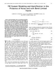
waveform, which we call the speech signal. <strong>Speech</strong> signals, as illustrated<br />
in Figure 1.1, can be converted <strong>to</strong> an electrical waveform by<br />
a microphone, further manipulated by both analog <strong>and</strong> digital signal<br />
processing, <strong>and</strong> then converted back <strong>to</strong> acoustic form by a loudspeaker,<br />
a telephone h<strong>and</strong>set or headphone, as desired. This form of speech processing<br />
is, of course, the basis for Bell’s telephone invention as well as<br />
<strong>to</strong>day’s multitude of devices for recording, transmitting, <strong>and</strong> manipulating<br />
speech <strong>and</strong> audio signals. Although Bell made his invention<br />
without knowing the fundamentals of information theory, these ideas<br />
3
4 <strong>Introduction</strong><br />
0<br />
0.12<br />
0.24<br />
0.36<br />
0.48<br />
SH<br />
0 0.02 0.04 0.06<br />
time in seconds<br />
0.08 0.1 0.12<br />
UH<br />
D W IY<br />
Fig. 1.1 A speech waveform with phonetic labels for the text message “Should we chase.”<br />
have assumed great importance in the design of sophisticated modern<br />
communications systems. Therefore, even though our main focus will<br />
be mostly on the speech waveform <strong>and</strong> its representation in the form of<br />
parametric models, it is nevertheless useful <strong>to</strong> begin with a discussion<br />
of how information is encoded in the speech waveform.<br />
1.1 The <strong>Speech</strong> Chain<br />
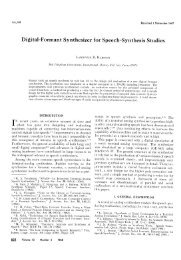
Figure 1.2 shows the complete process of producing <strong>and</strong> perceiving<br />
speech from the formulation of a message in the brain of a talker, <strong>to</strong><br />
the creation of the speech signal, <strong>and</strong> finally <strong>to</strong> the underst<strong>and</strong>ing of<br />
the message by a listener. In their classic introduction <strong>to</strong> speech science,<br />
Denes <strong>and</strong> Pinson aptly referred <strong>to</strong> this process as the “speech<br />
chain” [29]. The process starts in the upper left as a message represented<br />
somehow in the brain of the speaker. The message information<br />
can be thought of as having a number of different representations during<br />
the process of speech production (the upper path in Figure 1.2).<br />
S<br />
EY<br />
CH
text<br />
Message<br />
Formulation<br />
semantics<br />
Message<br />
Underst<strong>and</strong>ing<br />
phonemes,<br />
prosody<br />
Language<br />
Code<br />
phonemes, words<br />
sentences<br />
Language<br />
Translation<br />
<strong>Speech</strong> Production<br />
Neuro-Muscular<br />
Controls<br />
discrete input continuous input<br />
discrete output<br />
articula<strong>to</strong>ry motions<br />
feature<br />
extraction<br />
Neural<br />
Transduction<br />
continuous output<br />
<strong>Speech</strong> Perception<br />
1.1 The <strong>Speech</strong> Chain 5<br />
excitation,<br />
formants<br />
Vocal Tract<br />
System<br />
50 bps 200 bps 2000 bps 64-700 Kbps<br />
information rate<br />
spectrum<br />
analysis<br />
Basilar<br />
Membrane<br />
Motion<br />
acoustic<br />
waveform<br />
Transmission<br />
Channel<br />
acoustic<br />
waveform<br />
Fig. 1.2 The <strong>Speech</strong> Chain: from message, <strong>to</strong> speech signal, <strong>to</strong> underst<strong>and</strong>ing.<br />
For example the message could be represented initially as English text.<br />
In order <strong>to</strong> “speak” the message, the talker implicitly converts the text<br />
in<strong>to</strong> a symbolic representation of the sequence of sounds corresponding<br />
<strong>to</strong> the spoken version of the text. This step, called the language code<br />
genera<strong>to</strong>r in Figure 1.2, converts text symbols <strong>to</strong> phonetic symbols<br />
(along with stress <strong>and</strong> durational information) that describe the basic<br />
sounds of a spoken version of the message <strong>and</strong> the manner (i.e., the<br />
speed <strong>and</strong> emphasis) in which the sounds are intended <strong>to</strong> be produced.<br />
As an example, the segments of the waveform of Figure 1.1 are labeled<br />
with phonetic symbols using a computer-keyboard-friendly code called<br />
ARPAbet. 1 Thus, the text “should we chase” is represented phonetically<br />
(in ARPAbet symbols) as [SH UH D — W IY — CH EY S]. (See<br />
Chapter 2 for more discussion of phonetic transcription.) The third step<br />
in the speech production process is the conversion <strong>to</strong> “neuro-muscular<br />
controls,” i.e., the set of control signals that direct the neuro-muscular<br />
system <strong>to</strong> move the speech articula<strong>to</strong>rs, namely the <strong>to</strong>ngue, lips, teeth,<br />
1 The International Phonetic Association (IPA) provides a set of rules for phonetic transcription<br />
using an equivalent set of specialized symbols. The ARPAbet code does not<br />
require special fonts <strong>and</strong> is thus more convenient for computer applications.
6 <strong>Introduction</strong><br />
jaw <strong>and</strong> velum, in a manner that is consistent with the sounds of the<br />
desired spoken message <strong>and</strong> with the desired degree of emphasis. The<br />
end result of the neuro-muscular controls step is a set of articula<strong>to</strong>ry<br />
motions (continuous control) that cause the vocal tract articula<strong>to</strong>rs <strong>to</strong><br />
move in a prescribed manner in order <strong>to</strong> create the desired sounds.<br />
Finally the last step in the <strong>Speech</strong> Production process is the “vocal<br />
tract system” that physically creates the necessary sound sources <strong>and</strong><br />
the appropriate vocal tract shapes over time so as <strong>to</strong> create an acoustic<br />
waveform, such as the one shown in Figure 1.1, that encodes the information<br />
in the desired message in<strong>to</strong> the speech signal.<br />
To determine the rate of information flow during speech production,<br />
assume that there are about 32 symbols (letters) in the language<br />
(in English there are 26 letters, but if we include simple punctuation<br />
we get a count closer <strong>to</strong> 32 = 2 5 symbols). Furthermore, the rate of<br />
speaking for most people is about 10 symbols per second (somewhat<br />
on the high side, but still acceptable for a rough information rate estimate).<br />
Hence, assuming independent letters as a simple approximation,<br />
we estimate the base information rate of the text message as about<br />
50 bps (5 bits per symbol times 10 symbols per second). At the second<br />
stage of the process, where the text representation is converted in<strong>to</strong><br />
phonemes <strong>and</strong> prosody (e.g., pitch <strong>and</strong> stress) markers, the information<br />
rate is estimated <strong>to</strong> increase by a fac<strong>to</strong>r of 4 <strong>to</strong> about 200 bps. For<br />
example, the ARBAbet phonetic symbol set used <strong>to</strong> label the speech<br />
sounds in Figure 1.1 contains approximately 64 = 2 6 symbols, or about<br />
6 bits/phoneme (again a rough approximation assuming independence<br />
of phonemes). In Figure 1.1, there are 8 phonemes in approximately<br />
600 ms. This leads <strong>to</strong> an estimate of 8 × 6/0.6 = 80 bps. Additional<br />
information required <strong>to</strong> describe prosodic features of the signal (e.g.,<br />
duration, pitch, loudness) could easily add 100 bps <strong>to</strong> the <strong>to</strong>tal information<br />
rate for a message encoded as a speech signal.<br />
The information representations for the first two stages in the speech<br />
chain are discrete so we can readily estimate the rate of information<br />
flow with some simple assumptions. For the next stage in the speech<br />
production part of the speech chain, the representation becomes continuous<br />
(in the form of control signals for articula<strong>to</strong>ry motion). If they<br />
could be measured, we could estimate the spectral b<strong>and</strong>width of these
1.1 The <strong>Speech</strong> Chain 7<br />
control signals <strong>and</strong> appropriately sample <strong>and</strong> quantize these signals <strong>to</strong><br />
obtain equivalent digital signals for which the data rate could be estimated.<br />
The articula<strong>to</strong>rs move relatively slowly compared <strong>to</strong> the time<br />
variation of the resulting acoustic waveform. Estimates of b<strong>and</strong>width<br />
<strong>and</strong> required accuracy suggest that the <strong>to</strong>tal data rate of the sampled<br />
articula<strong>to</strong>ry control signals is about 2000 bps [34]. Thus, the original<br />
text message is represented by a set of continuously varying signals<br />
whose digital representation requires a much higher data rate than<br />
the information rate that we estimated for transmission of the message<br />
as a speech signal. 2 Finally, as we will see later, the data rate<br />
of the digitized speech waveform at the end of the speech production<br />
part of the speech chain can be anywhere from 64,000 <strong>to</strong> more than<br />
700,000 bps. We arrive at such numbers by examining the sampling<br />
rate <strong>and</strong> quantization required <strong>to</strong> represent the speech signal with a<br />
desired perceptual fidelity. For example, “telephone quality” requires<br />
that a b<strong>and</strong>width of 0–4 kHz be preserved, implying a sampling rate of<br />
8000 samples/s. Each sample can be quantized with 8 bits on a log scale,<br />
resulting in a bit rate of 64,000 bps. This representation is highly intelligible<br />
(i.e., humans can readily extract the message from it) but <strong>to</strong> most<br />
listeners, it will sound different from the original speech signal uttered<br />
by the talker. On the other h<strong>and</strong>, the speech waveform can be represented<br />
with “CD quality” using a sampling rate of 44,100 samples/s<br />
with 16 bit samples, or a data rate of 705,600 bps. In this case, the<br />
reproduced acoustic signal will be virtually indistinguishable from the<br />
original speech signal.<br />
As we move from text <strong>to</strong> speech waveform through the speech chain,<br />
the result is an encoding of the message that can be effectively transmitted<br />
by acoustic wave propagation <strong>and</strong> robustly decoded by the hearing<br />
mechanism of a listener. The above analysis of data rates shows<br />
that as we move from text <strong>to</strong> sampled speech waveform, the data rate<br />
can increase by a fac<strong>to</strong>r of 10,000. Part of this extra information represents<br />
characteristics of the talker such as emotional state, speech<br />
mannerisms, accent, etc., but much of it is due <strong>to</strong> the inefficiency<br />
2 Note that we introduce the term data rate for digital representations <strong>to</strong> distinguish from<br />
the inherent information content of the message represented by the speech signal.
8 <strong>Introduction</strong><br />
of simply sampling <strong>and</strong> finely quantizing analog signals. Thus, motivated<br />
by an awareness of the low intrinsic information rate of speech,<br />
a central theme of much of digital speech processing is <strong>to</strong> obtain a<br />
digital representation with lower data rate than that of the sampled<br />
waveform.<br />
The complete speech chain consists of a speech production/<br />
generation model, of the type discussed above, as well as a speech<br />
perception/recognition model, as shown progressing <strong>to</strong> the left in the<br />
bot<strong>to</strong>m half of Figure 1.2. The speech perception model shows the series<br />
of steps from capturing speech at the ear <strong>to</strong> underst<strong>and</strong>ing the message<br />
encoded in the speech signal. The first step is the effective conversion<br />
of the acoustic waveform <strong>to</strong> a spectral representation. This is<br />
done within the inner ear by the basilar membrane, which acts as a<br />
non-uniform spectrum analyzer by spatially separating the spectral<br />
components of the incoming speech signal <strong>and</strong> thereby analyzing them<br />
by what amounts <strong>to</strong> a non-uniform filter bank. The next step in the<br />
speech perception process is a neural transduction of the spectral features<br />
in<strong>to</strong> a set of sound features (or distinctive features as they are<br />
referred <strong>to</strong> in the area of linguistics) that can be decoded <strong>and</strong> processed<br />
by the brain. The next step in the process is a conversion of the sound<br />
features in<strong>to</strong> the set of phonemes, words, <strong>and</strong> sentences associated with<br />
the in-coming message by a language translation process in the human<br />
brain. Finally, the last step in the speech perception model is the conversion<br />
of the phonemes, words <strong>and</strong> sentences of the message in<strong>to</strong> an<br />
underst<strong>and</strong>ing of the meaning of the basic message in order <strong>to</strong> be able<br />
<strong>to</strong> respond <strong>to</strong> or take some appropriate action. Our fundamental underst<strong>and</strong>ing<br />
of the processes in most of the speech perception modules in<br />
Figure 1.2 is rudimentary at best, but it is generally agreed that some<br />
physical correlate of each of the steps in the speech perception model<br />
occur within the human brain, <strong>and</strong> thus the entire model is useful for<br />
thinking about the processes that occur.<br />
There is one additional process shown in the diagram of the complete<br />
speech chain in Figure 1.2 that we have not discussed — namely<br />
the transmission channel between the speech generation <strong>and</strong> speech<br />
perception parts of the model. In its simplest embodiment, this transmission<br />
channel consists of just the acoustic wave connection between
1.2 Applications of <strong>Digital</strong> <strong>Speech</strong> <strong>Processing</strong> 9<br />
a speaker <strong>and</strong> a listener who are in a common space. It is essential<br />
<strong>to</strong> include this transmission channel in our model for the speech<br />
chain since it includes real world noise <strong>and</strong> channel dis<strong>to</strong>rtions that<br />
make speech <strong>and</strong> message underst<strong>and</strong>ing more difficult in real communication<br />
environments. More interestingly for our purpose here —<br />
it is in this domain that we find the applications of digital speech<br />
processing.<br />
1.2 Applications of <strong>Digital</strong> <strong>Speech</strong> <strong>Processing</strong><br />
The first step in most applications of digital speech processing is <strong>to</strong><br />
convert the acoustic waveform <strong>to</strong> a sequence of numbers. Most modern<br />
A-<strong>to</strong>-D converters operate by sampling at a very high rate, applying a<br />
digital lowpass filter with cu<strong>to</strong>ff set <strong>to</strong> preserve a prescribed b<strong>and</strong>width,<br />
<strong>and</strong> then reducing the sampling rate <strong>to</strong> the desired sampling rate, which<br />
can be as low as twice the cu<strong>to</strong>ff frequency of the sharp-cu<strong>to</strong>ff digital<br />
filter. This discrete-time representation is the starting point for most<br />
applications. From this point, other representations are obtained by<br />
digital processing. For the most part, these alternative representations<br />
are based on incorporating knowledge about the workings of the speech<br />
chain as depicted in Figure 1.2. As we will see, it is possible <strong>to</strong> incorporate<br />
aspects of both the speech production <strong>and</strong> speech perception<br />
process in<strong>to</strong> the digital representation <strong>and</strong> processing. It is not an oversimplification<br />
<strong>to</strong> assert that digital speech processing is grounded in a<br />
set of techniques that have the goal of pushing the data rate of the<br />
speech representation <strong>to</strong> the left along either the upper or lower path<br />
in Figure 1.2.<br />
The remainder of this chapter is devoted <strong>to</strong> a brief summary of the<br />
applications of digital speech processing, i.e., the systems that people<br />
interact with daily. Our discussion will confirm the importance of the<br />
digital representation in all application areas.<br />
1.2.1 <strong>Speech</strong> Coding<br />
Perhaps the most widespread applications of digital speech processing<br />
technology occur in the areas of digital transmission <strong>and</strong> s<strong>to</strong>rage
10 <strong>Introduction</strong><br />
speech<br />
signal<br />
xc (t)<br />
A-<strong>to</strong>-D<br />
Converter<br />
samples<br />
x [n]<br />
Analysis/<br />
Encoding<br />
data<br />
y[n]<br />
decoded<br />
signal<br />
xc (t)<br />
D-<strong>to</strong>-A<br />
Converter<br />
samples data<br />
Synthesis/<br />
x[n]<br />
Decoding y[n]<br />
Fig. 1.3 <strong>Speech</strong> coding block diagram — encoder <strong>and</strong> decoder.<br />
Channel or<br />
Medium<br />
of speech signals. In these areas the centrality of the digital representation<br />
is obvious, since the goal is <strong>to</strong> compress the digital waveform<br />
representation of speech in<strong>to</strong> a lower bit-rate representation. It<br />
is common <strong>to</strong> refer <strong>to</strong> this activity as “speech coding” or “speech<br />
compression.”<br />
Figure 1.3 shows a block diagram of a generic speech encoding/decoding<br />
(or compression) system. In the upper part of the figure,<br />
the A-<strong>to</strong>-D converter converts the analog speech signal xc(t) <strong>to</strong> a sampled<br />
waveform representation x[n]. The digital signal x[n] is analyzed<br />
<strong>and</strong> coded by digital computation algorithms <strong>to</strong> produce a new digital<br />
signal y[n] that can be transmitted over a digital communication channel<br />
or s<strong>to</strong>red in a digital s<strong>to</strong>rage medium as ˆy[n]. As we will see, there<br />
are a myriad of ways <strong>to</strong> do the encoding so as <strong>to</strong> reduce the data rate<br />
over that of the sampled <strong>and</strong> quantized speech waveform x[n]. Because<br />
the digital representation at this point is often not directly related <strong>to</strong><br />
the sampled speech waveform, y[n] <strong>and</strong> ˆy[n] are appropriately referred<br />
<strong>to</strong> as data signals that represent the speech signal. The lower path in<br />
Figure 1.3 shows the decoder associated with the speech coder. The<br />
received data signal ˆy[n] is decoded using the inverse of the analysis<br />
processing, giving the sequence of samples ˆx[n] which is then converted<br />
(using a D-<strong>to</strong>-A Converter) back <strong>to</strong> an analog signal ˆxc(t) for human<br />
listening. The decoder is often called a synthesizer because it must<br />
reconstitute the speech waveform from data that may bear no direct<br />
relationship <strong>to</strong> the waveform.
1.2 Applications of <strong>Digital</strong> <strong>Speech</strong> <strong>Processing</strong> 11<br />
With carefully designed error protection coding of the digital<br />
representation, the transmitted (y[n]) <strong>and</strong> received (ˆy[n]) data can be<br />
essentially identical. This is the quintessential feature of digital coding.<br />
In theory, perfect transmission of the coded digital representation is<br />
possible even under very noisy channel conditions, <strong>and</strong> in the case of<br />
digital s<strong>to</strong>rage, it is possible <strong>to</strong> s<strong>to</strong>re a perfect copy of the digital representation<br />
in perpetuity if sufficient care is taken <strong>to</strong> update the s<strong>to</strong>rage<br />
medium as s<strong>to</strong>rage technology advances. This means that the speech<br />
signal can be reconstructed <strong>to</strong> within the accuracy of the original coding<br />
for as long as the digital representation is retained. In either case,<br />
the goal of the speech coder is <strong>to</strong> start with samples of the speech signal<br />
<strong>and</strong> reduce (compress) the data rate required <strong>to</strong> represent the speech<br />
signal while maintaining a desired perceptual fidelity. The compressed<br />
representation can be more efficiently transmitted or s<strong>to</strong>red, or the bits<br />
saved can be devoted <strong>to</strong> error protection.<br />
<strong>Speech</strong> coders enable a broad range of applications including narrowb<strong>and</strong><br />
<strong>and</strong> broadb<strong>and</strong> wired telephony, cellular communications,<br />
voice over internet pro<strong>to</strong>col (VoIP) (which utilizes the internet as<br />
a real-time communications medium), secure voice for privacy <strong>and</strong><br />
encryption (for national security applications), extremely narrowb<strong>and</strong><br />
communications channels (such as battlefield applications using high<br />
frequency (HF) radio), <strong>and</strong> for s<strong>to</strong>rage of speech for telephone answering<br />
machines, interactive voice response (IVR) systems, <strong>and</strong> prerecorded<br />
messages. <strong>Speech</strong> coders often utilize many aspects of both<br />
the speech production <strong>and</strong> speech perception processes, <strong>and</strong> hence may<br />
not be useful for more general audio signals such as music. Coders that<br />
are based on incorporating only aspects of sound perception generally<br />
do not achieve as much compression as those based on speech production,<br />
but they are more general <strong>and</strong> can be used for all types of audio<br />
signals. These coders are widely deployed in MP3 <strong>and</strong> AAC players <strong>and</strong><br />
for audio in digital television systems [120].<br />
1.2.2 Text-<strong>to</strong>-<strong>Speech</strong> Synthesis<br />
For many years, scientists <strong>and</strong> engineers have studied the speech production<br />
process with the goal of building a system that can start with
12 <strong>Introduction</strong><br />
text<br />
Linguistic<br />
Rules<br />
Synthesis<br />
Algorithm<br />
Fig. 1.4 Text-<strong>to</strong>-speech synthesis system block diagram.<br />
D-<strong>to</strong>-A<br />
Converter<br />
speech<br />
text <strong>and</strong> produce speech au<strong>to</strong>matically. In a sense, a text-<strong>to</strong>-speech<br />
synthesizer such as depicted in Figure 1.4 is a digital simulation of the<br />
entire upper part of the speech chain diagram. The input <strong>to</strong> the system<br />
is ordinary text such as an email message or an article from a newspaper<br />
or magazine. The first block in the text-<strong>to</strong>-speech synthesis system,<br />
labeled linguistic rules, has the job of converting the printed text input<br />
in<strong>to</strong> a set of sounds that the machine must synthesize. The conversion<br />
from text <strong>to</strong> sounds involves a set of linguistic rules that must determine<br />
the appropriate set of sounds (perhaps including things like emphasis,<br />
pauses, rates of speaking, etc.) so that the resulting synthetic speech<br />
will express the words <strong>and</strong> intent of the text message in what passes<br />
for a natural voice that can be decoded accurately by human speech<br />
perception. This is more difficult than simply looking up the words in<br />
a pronouncing dictionary because the linguistic rules must determine<br />
how <strong>to</strong> pronounce acronyms, how <strong>to</strong> pronounce ambiguous words like<br />
read, bass, object, how <strong>to</strong> pronounce abbreviations like St. (street or<br />
Saint), Dr. (Doc<strong>to</strong>r or drive), <strong>and</strong> how <strong>to</strong> properly pronounce proper<br />
names, specialized terms, etc. Once the proper pronunciation of the<br />
text has been determined, the role of the synthesis algorithm is <strong>to</strong> create<br />
the appropriate sound sequence <strong>to</strong> represent the text message in<br />
the form of speech. In essence, the synthesis algorithm must simulate<br />
the action of the vocal tract system in creating the sounds of speech.<br />
There are many procedures for assembling the speech sounds <strong>and</strong> compiling<br />
them in<strong>to</strong> a proper sentence, but the most promising one <strong>to</strong>day is<br />
called “unit selection <strong>and</strong> concatenation.” In this method, the computer<br />
s<strong>to</strong>res multiple versions of each of the basic units of speech (phones, half<br />
phones, syllables, etc.), <strong>and</strong> then decides which sequence of speech units<br />
sounds best for the particular text message that is being produced. The<br />
basic digital representation is not generally the sampled speech wave.<br />
Instead, some sort of compressed representation is normally used <strong>to</strong>
1.2 Applications of <strong>Digital</strong> <strong>Speech</strong> <strong>Processing</strong> 13<br />
save memory <strong>and</strong>, more importantly, <strong>to</strong> allow convenient manipulation<br />
of durations <strong>and</strong> blending of adjacent sounds. Thus, the speech synthesis<br />
algorithm would include an appropriate decoder, as discussed in<br />
Section 1.2.1, whose output is converted <strong>to</strong> an analog representation<br />
via the D-<strong>to</strong>-A converter.<br />
Text-<strong>to</strong>-speech synthesis systems are an essential component of<br />
modern human–machine communications systems <strong>and</strong> are used <strong>to</strong> do<br />
things like read email messages over a telephone, provide voice output<br />
from GPS systems in au<strong>to</strong>mobiles, provide the voices for talking<br />
agents for completion of transactions over the internet, h<strong>and</strong>le call center<br />
help desks <strong>and</strong> cus<strong>to</strong>mer care applications, serve as the voice for<br />
providing information from h<strong>and</strong>held devices such as foreign language<br />
phrasebooks, dictionaries, crossword puzzle helpers, <strong>and</strong> as the voice of<br />
announcement machines that provide information such as s<strong>to</strong>ck quotes,<br />
airline schedules, updates on arrivals <strong>and</strong> departures of flights, etc.<br />
Another important application is in reading machines for the blind,<br />
where an optical character recognition system provides the text input<br />
<strong>to</strong> a speech synthesis system.<br />
1.2.3 <strong>Speech</strong> Recognition <strong>and</strong> Other Pattern<br />
Matching Problems<br />
Another large class of digital speech processing applications is concerned<br />
with the au<strong>to</strong>matic extraction of information from the speech<br />
signal. Most such systems involve some sort of pattern matching.<br />
Figure 1.5 shows a block diagram of a generic approach <strong>to</strong> pattern<br />
matching problems in speech processing. Such problems include the<br />
following: speech recognition, where the object is <strong>to</strong> extract the message<br />
from the speech signal; speaker recognition, where the goal is<br />
<strong>to</strong> identify who is speaking; speaker verification, where the goal is<br />
<strong>to</strong> verify a speaker’s claimed identity from analysis of their speech<br />
speech<br />
A-<strong>to</strong>-D<br />
Converter<br />
Feature<br />
Analysis<br />
Pattern<br />
Matching<br />
Fig. 1.5 Block diagram of general pattern matching system for speech signals.<br />
symbols
14 <strong>Introduction</strong><br />
signal; word spotting, which involves moni<strong>to</strong>ring a speech signal for<br />
the occurrence of specified words or phrases; <strong>and</strong> au<strong>to</strong>matic indexing<br />
of speech recordings based on recognition (or spotting) of spoken<br />
keywords.<br />
The first block in the pattern matching system converts the analog<br />
speech waveform <strong>to</strong> digital form using an A-<strong>to</strong>-D converter. The<br />
feature analysis module converts the sampled speech signal <strong>to</strong> a set<br />
of feature vec<strong>to</strong>rs. Often, the same analysis techniques that are used<br />
in speech coding are also used <strong>to</strong> derive the feature vec<strong>to</strong>rs. The final<br />
block in the system, namely the pattern matching block, dynamically<br />
time aligns the set of feature vec<strong>to</strong>rs representing the speech signal with<br />
a concatenated set of s<strong>to</strong>red patterns, <strong>and</strong> chooses the identity associated<br />
with the pattern which is the closest match <strong>to</strong> the time-aligned set<br />
of feature vec<strong>to</strong>rs of the speech signal. The symbolic output consists<br />
of a set of recognized words, in the case of speech recognition, or the<br />
identity of the best matching talker, in the case of speaker recognition,<br />
or a decision as <strong>to</strong> whether <strong>to</strong> accept or reject the identity claim of a<br />
speaker in the case of speaker verification.<br />
Although the block diagram of Figure 1.5 represents a wide range<br />
of speech pattern matching problems, the biggest use has been in the<br />
area of recognition <strong>and</strong> underst<strong>and</strong>ing of speech in support of human–<br />
machine communication by voice. The major areas where such a system<br />
finds applications include comm<strong>and</strong> <strong>and</strong> control of computer software,<br />
voice dictation <strong>to</strong> create letters, memos, <strong>and</strong> other documents, natural<br />
language voice dialogues with machines <strong>to</strong> enable help desks <strong>and</strong><br />
call centers, <strong>and</strong> for agent services such as calendar entry <strong>and</strong> update,<br />
address list modification <strong>and</strong> entry, etc.<br />
Pattern recognition applications often occur in conjunction with<br />
other digital speech processing applications. For example, one of the<br />
preeminent uses of speech technology is in portable communication<br />
devices. <strong>Speech</strong> coding at bit rates on the order of 8 Kbps enables normal<br />
voice conversations in cell phones. Spoken name speech recognition<br />
in cellphones enables voice dialing capability that can au<strong>to</strong>matically<br />
dial the number associated with the recognized name. Names from<br />
direc<strong>to</strong>ries with upwards of several hundred names can readily be recognized<br />
<strong>and</strong> dialed using simple speech recognition technology.
1.2 Applications of <strong>Digital</strong> <strong>Speech</strong> <strong>Processing</strong> 15<br />
Another major speech application that has long been a dream<br />
of speech researchers is au<strong>to</strong>matic language translation. The goal of<br />
language translation systems is <strong>to</strong> convert spoken words in one language<br />
<strong>to</strong> spoken words in another language so as <strong>to</strong> facilitate natural<br />
language voice dialogues between people speaking different languages.<br />
Language translation technology requires speech synthesis systems that<br />
work in both languages, along with speech recognition (<strong>and</strong> generally<br />
natural language underst<strong>and</strong>ing) that also works for both languages;<br />
hence it is a very difficult task <strong>and</strong> one for which only limited progress<br />
has been made. When such systems exist, it will be possible for people<br />
speaking different languages <strong>to</strong> communicate at data rates on the order<br />
of that of printed text reading!<br />
1.2.4 Other <strong>Speech</strong> Applications<br />
The range of speech communication applications is illustrated in<br />
Figure 1.6. As seen in this figure, the techniques of digital speech<br />
processing are a key ingredient of a wide range of applications that<br />
include the three areas of transmission/s<strong>to</strong>rage, speech synthesis, <strong>and</strong><br />
speech recognition as well as many others such as speaker identification,<br />
speech signal quality enhancement, <strong>and</strong> aids for the hearing- or visuallyimpaired.<br />
The block diagram in Figure 1.7 represents any system where time<br />
signals such as speech are processed by the techniques of DSP. This<br />
figure simply depicts the notion that once the speech signal is sampled,<br />
it can be manipulated in virtually limitless ways by DSP techniques.<br />
Here again, manipulations <strong>and</strong> modifications of the speech signal are<br />
<strong>Digital</strong><br />
Transmission<br />
& S<strong>to</strong>rage<br />
<strong>Speech</strong><br />
Synthesis<br />
<strong>Digital</strong> <strong>Speech</strong> <strong>Processing</strong><br />
Techniques<br />
<strong>Speech</strong><br />
Recognition<br />
Speaker<br />
Verification/<br />
Identification<br />
Fig. 1.6 Range of speech communication applications.<br />
Enhancement<br />
of <strong>Speech</strong><br />
Quality<br />
Aids for the<br />
H<strong>and</strong>icapped
16 <strong>Introduction</strong><br />
speech<br />
A-<strong>to</strong>-D<br />
Converter<br />
<strong>Computer</strong><br />
Algorithm<br />
D-<strong>to</strong>-A<br />
Converter<br />
speech<br />
Fig. 1.7 General block diagram for application of digital signal processing <strong>to</strong> speech signals.<br />
usually achieved by transforming the speech signal in<strong>to</strong> an alternative<br />
representation (that is motivated by our underst<strong>and</strong>ing of speech production<br />
<strong>and</strong> speech perception), operating on that representation by<br />
further digital computation, <strong>and</strong> then transforming back <strong>to</strong> the waveform<br />
domain, using a D-<strong>to</strong>-A converter.<br />
One important application area is speech enhancement, where the<br />
goal is <strong>to</strong> remove or suppress noise or echo or reverberation picked up by<br />
a microphone along with the desired speech signal. In human-<strong>to</strong>-human<br />
communication, the goal of speech enhancement systems is <strong>to</strong> make the<br />
speech more intelligible <strong>and</strong> more natural; however, in reality the best<br />
that has been achieved so far is less perceptually annoying speech that<br />
essentially maintains, but does not improve, the intelligibility of the<br />
noisy speech. Success has been achieved, however, in making dis<strong>to</strong>rted<br />
speech signals more useful for further processing as part of a speech<br />
coder, synthesizer, or recognizer. An excellent reference in this area is<br />
the recent textbook by Loizou [72].<br />
Other examples of manipulation of the speech signal include<br />
timescale modification <strong>to</strong> align voices with video segments, <strong>to</strong> modify<br />
voice qualities, <strong>and</strong> <strong>to</strong> speed-up or slow-down prerecorded speech<br />
(e.g., for talking books, rapid review of voice mail messages, or careful<br />
scrutinizing of spoken material).<br />
1.3 Our Goal for this Text<br />
We have discussed the speech signal <strong>and</strong> how it encodes information<br />
for human communication. We have given a brief overview of the way<br />
in which digital speech processing is being applied <strong>to</strong>day, <strong>and</strong> we have<br />
hinted at some of the possibilities that exist for the future. These <strong>and</strong><br />
many more examples all rely on the basic principles of digital speech<br />
processing, which we will discuss in the remainder of this text. We<br />
make no pretense of exhaustive coverage. The subject is <strong>to</strong>o broad <strong>and</strong>
1.3 Our Goal for this Text 17<br />
<strong>to</strong>o deep. Our goal is only <strong>to</strong> provide an up-<strong>to</strong>-date introduction <strong>to</strong> this<br />
fascinating field. We will not be able <strong>to</strong> go in<strong>to</strong> great depth, <strong>and</strong> we will<br />
not be able <strong>to</strong> cover all the possible applications of digital speech processing<br />
techniques. Instead our focus is on the fundamentals of digital<br />
speech processing <strong>and</strong> their application <strong>to</strong> coding, synthesis, <strong>and</strong> recognition.<br />
This means that some of the latest algorithmic innovations <strong>and</strong><br />
applications will not be discussed — not because they are not interesting,<br />
but simply because there are so many fundamental tried-<strong>and</strong>-true<br />
techniques that remain at the core of digital speech processing. We<br />
hope that this text will stimulate readers <strong>to</strong> investigate the subject in<br />
greater depth using the extensive set of references provided.
2<br />
The <strong>Speech</strong> Signal<br />
As the discussion in Chapter 1 shows, the goal in many applications of<br />
digital speech processing techniques is <strong>to</strong> move the digital representation<br />
of the speech signal from the waveform samples back up the speech<br />
chain <strong>to</strong>ward the message. To gain a better idea of what this means,<br />
this chapter provides a brief overview of the phonetic representation of<br />
speech <strong>and</strong> an introduction <strong>to</strong> models for the production of the speech<br />
signal.<br />
2.1 Phonetic Representation of <strong>Speech</strong><br />
<strong>Speech</strong> can be represented phonetically by a finite set of symbols called<br />
the phonemes of the language, the number of which depends upon the<br />
language <strong>and</strong> the refinement of the analysis. For most languages the<br />
number of phonemes is between 32 <strong>and</strong> 64. A condensed inven<strong>to</strong>ry of<br />
the sounds of speech in the English language is given in Table 2.1,<br />
where the phonemes are denoted by a set of ASCII symbols called the<br />
ARPAbet. Table 2.1 also includes some simple examples of ARPAbet<br />
transcriptions of words containing each of the phonemes of English.<br />
Additional phonemes can be added <strong>to</strong> Table 2.1 <strong>to</strong> account for allophonic<br />
variations <strong>and</strong> events such as glottal s<strong>to</strong>ps <strong>and</strong> pauses.<br />
18
2.1 Phonetic Representation of <strong>Speech</strong> 19<br />
Table 2.1 Condensed list of ARPAbet phonetic symbols for North American English.<br />
Class ARPAbet Example Transcription<br />
Vowels <strong>and</strong> IY beet [BIYT]<br />
diphthongs IH bit [BIHT]<br />
EY bait [BEYT]<br />
EH bet [BEHT]<br />
AE bat [BAET]<br />
AA bob [BAAB]<br />
AO born [B AO R N]<br />
UH book [BUHK]<br />
OW boat [BOWT]<br />
UW boot [BUWT]<br />
AH but [BAHT]<br />
ER bird [BERD]<br />
AY buy [B AY]<br />
AW down [DAWN]<br />
OY boy [B OY]<br />
Glides Y you [Y UH]<br />
R rent [REHNT]<br />
Liquids W wit [W IH T]<br />
L let [L EH T]<br />
Nasals M met [M EH T]<br />
N net [N EH T]<br />
NG sing [S IH NG]<br />
S<strong>to</strong>ps P pat [P AE T]<br />
B bet [B EH T]<br />
T ten [T EH N]<br />
D debt [D EH T]<br />
K kit [K IH T]<br />
G get [G EH T]<br />
Fricatives HH hat [HH AE T]<br />
F f at [F AE T]<br />
V vat [V AE T]<br />
TH thing [TH IH NG]<br />
DH that [DH AE T]<br />
S sat [S AE T]<br />
Z z oo [Z UW]<br />
SH shut [SH AH T]<br />
ZH az ure [AE ZH ER]<br />
Affricates CH chase [CH EY S]<br />
JH j udge [JH AH JH ]<br />
a This set of 39 phonemes is used in the CMU Pronouncing Dictionary available on-line at<br />
http://www.speech.cs.cmu.edu/cgi-bin/cmudict.<br />
Figure 1.1 on p. 4 shows how the sounds corresponding <strong>to</strong> the text<br />
“should we chase” are encoded in<strong>to</strong> a speech waveform. We see that, for<br />
the most part, phonemes have a distinctive appearance in the speech<br />
waveform. Thus sounds like /SH/ <strong>and</strong> /S/ look like (spectrally shaped)
20 The <strong>Speech</strong> Signal<br />
r<strong>and</strong>om noise, while the vowel sounds /UH/, /IY/, <strong>and</strong> /EY/ are highly<br />
structured <strong>and</strong> quasi-periodic. These differences result from the distinctively<br />
different ways that these sounds are produced.<br />
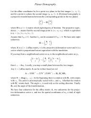
2.2 Models for <strong>Speech</strong> Production<br />
A schematic longitudinal cross-sectional drawing of the human vocal<br />
tract mechanism is given in Figure 2.1 [35]. This diagram highlights<br />
the essential physical features of human ana<strong>to</strong>my that enter in<strong>to</strong> the<br />
final stages of the speech production process. It shows the vocal tract<br />
as a tube of nonuniform cross-sectional area that is bounded at one end<br />
by the vocal cords <strong>and</strong> at the other by the mouth opening. This tube<br />
serves as an acoustic transmission system for sounds generated inside<br />
the vocal tract. For creating nasal sounds like /M/, /N/, or /NG/,<br />
a side-branch tube, called the nasal tract, is connected <strong>to</strong> the main<br />
acoustic branch by the trapdoor action of the velum. This branch path<br />
radiates sound at the nostrils. The shape (variation of cross-section<br />
along the axis) of the vocal tract varies with time due <strong>to</strong> motions of<br />
the lips, jaw, <strong>to</strong>ngue, <strong>and</strong> velum. Although the actual human vocal<br />
tract is not laid out along a straight line as in Figure 2.1, this type of<br />
model is a reasonable approximation for wavelengths of the sounds in<br />
speech.<br />
The sounds of speech are generated in the system of Figure 2.1 in<br />
several ways. Voiced sounds (vowels, liquids, glides, nasals in Table 2.1)<br />
Fig. 2.1 Schematic model of the vocal tract system. (After Flanagan et al. [35].)
2.2 Models for <strong>Speech</strong> Production 21<br />
are produced when the vocal tract tube is excited by pulses of air pressure<br />
resulting from quasi-periodic opening <strong>and</strong> closing of the glottal<br />
orifice (opening between the vocal cords). Examples in Figure 1.1 are<br />
the vowels /UH/, /IY/, <strong>and</strong> /EY/, <strong>and</strong> the liquid consonant /W/.<br />
Unvoiced sounds are produced by creating a constriction somewhere in<br />
the vocal tract tube <strong>and</strong> forcing air through that constriction, thereby<br />
creating turbulent air flow, which acts as a r<strong>and</strong>om noise excitation of<br />
the vocal tract tube. Examples are the unvoiced fricative sounds such as<br />
/SH/ <strong>and</strong> /S/. A third sound production mechanism is when the vocal<br />
tract is partially closed off causing turbulent flow due <strong>to</strong> the constriction,<br />
at the same time allowing quasi-periodic flow due <strong>to</strong> vocal cord<br />
vibrations. Sounds produced in this manner include the voiced fricatives<br />
/V/, /DH/, /Z/, <strong>and</strong> /ZH/. Finally, plosive sounds such as /P/,<br />
/T/, <strong>and</strong> /K/ <strong>and</strong> affricates such as /CH/ are formed by momentarily<br />
closing off air flow, allowing pressure <strong>to</strong> build up behind the closure, <strong>and</strong><br />
then abruptly releasing the pressure. All these excitation sources create<br />
a wide-b<strong>and</strong> excitation signal <strong>to</strong> the vocal tract tube, which acts as<br />
an acoustic transmission line with certain vocal tract shape-dependent<br />
resonances that tend <strong>to</strong> emphasize some frequencies of the excitation<br />
relative <strong>to</strong> others.<br />
As discussed in Chapter 1 <strong>and</strong> illustrated by the waveform in<br />
Figure 1.1, the general character of the speech signal varies at the<br />
phoneme rate, which is on the order of 10 phonemes per second, while<br />
the detailed time variations of the speech waveform are at a much higher<br />
rate. That is, the changes in vocal tract configuration occur relatively<br />
slowly compared <strong>to</strong> the detailed time variation of the speech signal. The<br />
sounds created in the vocal tract are shaped in the frequency domain<br />
by the frequency response of the vocal tract. The resonance frequencies<br />
resulting from a particular configuration of the articula<strong>to</strong>rs are instrumental<br />
in forming the sound corresponding <strong>to</strong> a given phoneme. These<br />
resonance frequencies are called the formant frequencies of the sound<br />
[32, 34]. In summary, the fine structure of the time waveform is created<br />
by the sound sources in the vocal tract, <strong>and</strong> the resonances of the vocal<br />
tract tube shape these sound sources in<strong>to</strong> the phonemes.<br />
The system of Figure 2.1 can be described by acoustic theory,<br />
<strong>and</strong> numerical techniques can be used <strong>to</strong> create a complete physical
22 The <strong>Speech</strong> Signal<br />
Excitation<br />
Parameters<br />
Vocal Tract<br />
Parameters<br />
Excitation<br />
Linear<br />
Genera<strong>to</strong>r excitation signal System speech signal<br />
Fig. 2.2 Source/system model for a speech signal.<br />
simulation of sound generation <strong>and</strong> transmission in the vocal tract<br />
[36, 93], but, for the most part, it is sufficient <strong>to</strong> model the production<br />
of a sampled speech signal by a discrete-time system model such<br />
as the one depicted in Figure 2.2. The discrete-time time-varying linear<br />
system on the right in Figure 2.2 simulates the frequency shaping of<br />
the vocal tract tube. The excitation genera<strong>to</strong>r on the left simulates the<br />
different modes of sound generation in the vocal tract. Samples of a<br />
speech signal are assumed <strong>to</strong> be the output of the time-varying linear<br />
system.<br />
In general such a model is called a source/system model of speech<br />
production. The short-time frequency response of the linear system<br />
simulates the frequency shaping of the vocal tract system, <strong>and</strong> since the<br />
vocal tract changes shape relatively slowly, it is reasonable <strong>to</strong> assume<br />
that the linear system response does not vary over time intervals on the<br />
order of 10 ms or so. Thus, it is common <strong>to</strong> characterize the discretetime<br />
linear system by a system function of the form:<br />
H(z)=<br />
1 −<br />
M<br />
k=0<br />
bkz −k<br />
N<br />
k=1<br />
akz −k<br />
=<br />
b0<br />
M<br />
(1 − dkz −1 )<br />
k=1<br />
N<br />
(1 − ckz −1 )<br />
k=1<br />
, (2.1)<br />
where the filter coefficients ak <strong>and</strong> bk (labeled as vocal tract parameters<br />
in Figure 2.2) change at a rate on the order of 50–100 times/s. Some<br />
of the poles (ck) of the system function lie close <strong>to</strong> the unit circle<br />
<strong>and</strong> create resonances <strong>to</strong> model the formant frequencies. In detailed<br />
modeling of speech production [32, 34, 64], it is sometimes useful <strong>to</strong><br />
employ zeros (dk) of the system function <strong>to</strong> model nasal <strong>and</strong> fricative
2.2 Models for <strong>Speech</strong> Production 23<br />
sounds. However, as we discuss further in Chapter 4, many applications<br />
of the source/system model only include poles in the model because this<br />
simplifies the analysis required <strong>to</strong> estimate the parameters of the model<br />
from the speech signal.<br />
The box labeled excitation genera<strong>to</strong>r in Figure 2.2 creates an appropriate<br />
excitation for the type of sound being produced. For voiced<br />
speech the excitation <strong>to</strong> the linear system is a quasi-periodic sequence<br />
of discrete (glottal) pulses that look very much like those shown in the<br />
righth<strong>and</strong> half of the excitation signal waveform in Figure 2.2. The fundamental<br />
frequency of the glottal excitation determines the perceived<br />
pitch of the voice. The individual finite-duration glottal pulses have a<br />
lowpass spectrum that depends on a number of fac<strong>to</strong>rs [105]. Therefore,<br />
the periodic sequence of smooth glottal pulses has a harmonic line<br />
spectrum with components that decrease in amplitude with increasing<br />
frequency. Often it is convenient <strong>to</strong> absorb the glottal pulse spectrum<br />
contribution in<strong>to</strong> the vocal tract system model of (2.1). This can be<br />
achieved by a small increase in the order of the denomina<strong>to</strong>r over what<br />
would be needed <strong>to</strong> represent the formant resonances. For unvoiced<br />
speech, the linear system is excited by a r<strong>and</strong>om number genera<strong>to</strong>r<br />
that produces a discrete-time noise signal with flat spectrum as shown<br />
in the left-h<strong>and</strong> half of the excitation signal. The excitation in Figure<br />
2.2 switches from unvoiced <strong>to</strong> voiced leading <strong>to</strong> the speech signal<br />
output as shown in the figure. In either case, the linear system imposes<br />
its frequency response on the spectrum <strong>to</strong> create the speech sounds.<br />
This model of speech as the output of a slowly time-varying digital<br />
filter with an excitation that captures the nature of the voiced/unvoiced<br />
distinction in speech production is the basis for thinking about the<br />
speech signal, <strong>and</strong> a wide variety of digital representations of the speech<br />
signal are based on it. That is, the speech signal is represented by the<br />
parameters of the model instead of the sampled waveform. By assuming<br />
that the properties of the speech signal (<strong>and</strong> the model) are constant<br />
over short time intervals, it is possible <strong>to</strong> compute/measure/estimate<br />
the parameters of the model by analyzing short blocks of samples of<br />
the speech signal. It is through such models <strong>and</strong> analysis techniques<br />
that we are able <strong>to</strong> build properties of the speech production process<br />
in<strong>to</strong> digital representations of the speech signal.
24 The <strong>Speech</strong> Signal<br />
2.3 More Refined Models<br />
Source/system models as shown in Figure 2.2 with the system characterized<br />
by a time-sequence of time-invariant systems are quite sufficient<br />
for most applications in speech processing, <strong>and</strong> we shall rely on<br />
such models throughout this text. However, such models are based on<br />
many approximations including the assumption that the source <strong>and</strong> the<br />
system do not interact, the assumption of linearity, <strong>and</strong> the assumption<br />
that the distributed continuous-time vocal tract transmission system<br />
can be modeled by a discrete linear time-invariant system. Fluid<br />
mechanics <strong>and</strong> acoustic wave propagation theory are fundamental physical<br />
principles that must be applied for detailed modeling of speech<br />
production. Since the early work of Flanagan <strong>and</strong> Ishizaka [34, 36, 51]<br />
much work has been devoted <strong>to</strong> creating detailed simulations of glottal<br />
flow, the interaction of the glottal source <strong>and</strong> the vocal tract in speech<br />
production, <strong>and</strong> the nonlinearities that enter in<strong>to</strong> sound generation <strong>and</strong><br />
transmission in the vocal tract. Stevens [121] <strong>and</strong> Quatieri [94] provide<br />
useful discussions of these effects. For many years, researchers have<br />
sought <strong>to</strong> measure the physical dimensions of the human vocal tract<br />
during speech production. This information is essential for detailed simulations<br />
based on acoustic theory. Early efforts <strong>to</strong> measure vocal tract<br />
area functions involved h<strong>and</strong> tracing on X-ray pictures [32]. Recent<br />
advances in MRI imaging <strong>and</strong> computer image analysis have provided<br />
significant advances in this area of speech science [17].
3<br />
Hearing <strong>and</strong> Audi<strong>to</strong>ry Perception<br />
In Chapter 2, we introduced the speech production process <strong>and</strong> showed<br />
how we could model speech production using discrete-time systems.<br />
In this chapter we turn <strong>to</strong> the perception side of the speech chain <strong>to</strong><br />
discuss properties of human sound perception that can be employed <strong>to</strong><br />
create digital representations of the speech signal that are perceptually<br />
robust.<br />
3.1 The Human Ear<br />
Figure 3.1 shows a schematic view of the human ear showing the three<br />
distinct sound processing sections, namely: the outer ear consisting of<br />
the pinna, which gathers sound <strong>and</strong> conducts it through the external<br />
canal <strong>to</strong> the middle ear; the middle ear beginning at the tympanic<br />
membrane, or eardrum, <strong>and</strong> including three small bones, the malleus<br />
(also called the hammer), the incus (also called the anvil) <strong>and</strong> the stapes<br />
(also called the stirrup), which perform a transduction from acoustic<br />
waves <strong>to</strong> mechanical pressure waves; <strong>and</strong> finally, the inner ear, which<br />
consists of the cochlea <strong>and</strong> the set of neural connections <strong>to</strong> the audi<strong>to</strong>ry<br />
nerve, which conducts the neural signals <strong>to</strong> the brain.<br />
25
26 Hearing <strong>and</strong> Audi<strong>to</strong>ry Perception<br />
Fig. 3.1 Schematic view of the human ear (inner <strong>and</strong> middle structures enlarged). (After<br />
Flanagan [34].)<br />
Figure 3.2 [107] depicts a block diagram abstraction of the audi<strong>to</strong>ry<br />
system. The acoustic wave is transmitted from the outer ear <strong>to</strong> the<br />
inner ear where the ear drum <strong>and</strong> bone structures convert the sound<br />
wave <strong>to</strong> mechanical vibrations which ultimately are transferred <strong>to</strong> the<br />
basilar membrane inside the cochlea. The basilar membrane vibrates in<br />
a frequency-selective manner along its extent <strong>and</strong> thereby performs a<br />
rough (non-uniform) spectral analysis of the sound. Distributed along<br />
Fig. 3.2 Schematic model of the audi<strong>to</strong>ry mechanism. (After Sachs et al. [107].)
3.2 Perception of Loudness 27<br />
the basilar membrane are a set of inner hair cells that serve <strong>to</strong> convert<br />
motion along the basilar membrane <strong>to</strong> neural activity. This produces<br />
an audi<strong>to</strong>ry nerve representation in both time <strong>and</strong> frequency. The processing<br />
at higher levels in the brain, shown in Figure 3.2 as a sequence<br />
of central processing with multiple representations followed by some<br />
type of pattern recognition, is not well unders<strong>to</strong>od <strong>and</strong> we can only<br />
postulate the mechanisms used by the human brain <strong>to</strong> perceive sound<br />
or speech. Even so, a wealth of knowledge about how sounds are perceived<br />
has been discovered by careful experiments that use <strong>to</strong>nes <strong>and</strong><br />
noise signals <strong>to</strong> stimulate the audi<strong>to</strong>ry system of human observers in<br />
very specific <strong>and</strong> controlled ways. These experiments have yielded much<br />
valuable knowledge about the sensitivity of the human audi<strong>to</strong>ry system<br />
<strong>to</strong> acoustic properties such as intensity <strong>and</strong> frequency.<br />
3.2 Perception of Loudness<br />
A key fac<strong>to</strong>r in the perception of speech <strong>and</strong> other sounds is loudness.<br />
Loudness is a perceptual quality that is related <strong>to</strong> the physical property<br />
of sound pressure level. Loudness is quantified by relating the actual<br />
sound pressure level of a pure <strong>to</strong>ne (in dB relative <strong>to</strong> a st<strong>and</strong>ard reference<br />
level) <strong>to</strong> the perceived loudness of the same <strong>to</strong>ne (in a unit called<br />
phons) over the range of human hearing (20 Hz–20 kHz). This relationship<br />
is shown in Figure 3.3 [37, 103]. These loudness curves show that<br />
the perception of loudness is frequency-dependent. Specifically, the dotted<br />
curve at the bot<strong>to</strong>m of the figure labeled “threshold of audibility”<br />
shows the sound pressure level that is required for a sound of a given<br />
frequency <strong>to</strong> be just audible (by a person with normal hearing). It can<br />
be seen that low frequencies must be significantly more intense than<br />
frequencies in the mid-range in order that they be perceived at all. The<br />
solid curves are equal-loudness-level con<strong>to</strong>urs measured by comparing<br />
sounds at various frequencies with a pure <strong>to</strong>ne of frequency 1000 Hz <strong>and</strong><br />
known sound pressure level. For example, the point at frequency 100 Hz<br />
on the curve labeled 50 (phons) is obtained by adjusting the power of<br />
the 100 Hz <strong>to</strong>ne until it sounds as loud as a 1000 Hz <strong>to</strong>ne having a sound<br />
pressure level of 50 dB. Careful measurements of this kind show that a<br />
100 Hz <strong>to</strong>ne must have a sound pressure level of about 60 dB in order
28 Hearing <strong>and</strong> Audi<strong>to</strong>ry Perception<br />
Fig. 3.3 Loudness level for human hearing. (After Fletcher <strong>and</strong> Munson [37].)<br />
<strong>to</strong> be perceived <strong>to</strong> be equal in loudness <strong>to</strong> the 1000 Hz <strong>to</strong>ne of sound<br />
pressure level 50 dB. By convention, both the 50 dB 1000 Hz <strong>to</strong>ne <strong>and</strong><br />
the 60 dB 100 Hz <strong>to</strong>ne are said <strong>to</strong> have a loudness level of 50 phons<br />
(pronounced as /F OW N Z/).<br />
The equal-loudness-level curves show that the audi<strong>to</strong>ry system is<br />
most sensitive for frequencies ranging from about 100 Hz up <strong>to</strong> about<br />
6 kHz with the greatest sensitivity at around 3 <strong>to</strong> 4 kHz. This is almost<br />
precisely the range of frequencies occupied by most of the sounds of<br />
speech.<br />
3.3 Critical B<strong>and</strong>s<br />
The non-uniform frequency analysis performed by the basilar membrane<br />
can be thought of as equivalent <strong>to</strong> that of a set of b<strong>and</strong>pass filters<br />
whose frequency responses become increasingly broad with increasing<br />
frequency. An idealized version of such a filter bank is depicted<br />
schematically in Figure 3.4. In reality, the b<strong>and</strong>pass filters are not ideal
amplitude<br />
3.4 Pitch Perception 29<br />
Fig. 3.4 Schematic representation of b<strong>and</strong>pass filters according <strong>to</strong> the critical b<strong>and</strong> theory<br />
of hearing.<br />
as shown in Figure 3.4, but their frequency responses overlap significantly<br />
since points on the basilar membrane cannot vibrate independently<br />
of each other. Even so, the concept of b<strong>and</strong>pass filter analysis<br />
in the cochlea is well established, <strong>and</strong> the critical b<strong>and</strong>widths have<br />
been defined <strong>and</strong> measured using a variety of methods, showing that<br />
the effective b<strong>and</strong>widths are constant at about 100 Hz for center frequencies<br />
below 500 Hz, <strong>and</strong> with a relative b<strong>and</strong>width of about 20%<br />
of the center frequency above 500 Hz. An equation that fits empirical<br />
measurements over the audi<strong>to</strong>ry range is<br />
∆fc =25+75[1+1.4(fc/1000) 2 ] 0.69 , (3.1)<br />
where ∆fc is the critical b<strong>and</strong>width associated with center frequency<br />
fc [134]. Approximately 25 critical b<strong>and</strong> filters span the range from<br />
0 <strong>to</strong> 20 kHz. The concept of critical b<strong>and</strong>s is very important in underst<strong>and</strong>ing<br />
such phenomena as loudness perception, pitch perception, <strong>and</strong><br />
masking, <strong>and</strong> it therefore provides motivation for digital representations<br />
of the speech signal that are based on a frequency decomposition.<br />
3.4 Pitch Perception<br />
Most musical sounds as well as voiced speech sounds have a periodic<br />
structure when viewed over short time intervals, <strong>and</strong> such sounds are<br />
perceived by the audi<strong>to</strong>ry system as having a quality known as pitch.<br />
Like loudness, pitch is a subjective attribute of sound that is related <strong>to</strong><br />
the fundamental frequency of the sound, which is a physical attribute of<br />
the acoustic waveform [122]. The relationship between pitch (measured
30 Hearing <strong>and</strong> Audi<strong>to</strong>ry Perception<br />
Fig. 3.5 Relation between subjective pitch <strong>and</strong> frequency of a pure <strong>to</strong>ne.<br />
on a nonlinear frequency scale called the mel-scale) <strong>and</strong> frequency of a<br />
pure <strong>to</strong>ne is approximated by the equation [122]:<br />
Pitch in mels = 1127log e(1 + f/700), (3.2)<br />
which is plotted in Figure 3.5. This expression is calibrated so that a<br />
frequency of 1000 Hz corresponds <strong>to</strong> a pitch of 1000 mels. This empirical<br />
scale describes the results of experiments where subjects were asked <strong>to</strong><br />
adjust the pitch of a measurement <strong>to</strong>ne <strong>to</strong> half the pitch of a reference<br />
<strong>to</strong>ne. To calibrate the scale, a <strong>to</strong>ne of frequency 1000 Hz is given a<br />
pitch of 1000 mels. Below 1000 Hz, the relationship between pitch <strong>and</strong><br />
frequency is nearly proportional. For higher frequencies, however, the<br />
relationship is nonlinear. For example, (3.2) shows that a frequency of<br />
f = 5000 Hz corresponds <strong>to</strong> a pitch of 2364 mels.<br />
The psychophysical phenomenon of pitch, as quantified by the melscale,<br />
can be related <strong>to</strong> the concept of critical b<strong>and</strong>s [134]. It turns out<br />
that more or less independently of the center frequency of the b<strong>and</strong>, one<br />
critical b<strong>and</strong>width corresponds <strong>to</strong> about 100 mels on the pitch scale.<br />
This is shown in Figure 3.5, where a critical b<strong>and</strong> of width ∆fc = 160 Hz<br />
centered on fc = 1000 Hz maps in<strong>to</strong> a b<strong>and</strong> of width 106 mels <strong>and</strong> a<br />
critical b<strong>and</strong> of width 100 Hz centered on 350 Hz maps in<strong>to</strong> a b<strong>and</strong> of<br />
width 107 mels. Thus, what we know about pitch perception reinforces<br />
the notion that the audi<strong>to</strong>ry system performs a frequency analysis that<br />
can be simulated with a bank of b<strong>and</strong>pass filters whose b<strong>and</strong>widths<br />
increase as center frequency increases.
3.5 Audi<strong>to</strong>ry Masking 31<br />
Voiced speech is quasi-periodic, but contains many frequencies. Nevertheless,<br />
many of the results obtained with pure <strong>to</strong>nes are relevant <strong>to</strong><br />
the perception of voice pitch as well. Often the term pitch period is used<br />
for the fundamental period of the voiced speech signal even though its<br />
usage in this way is somewhat imprecise.<br />
3.5 Audi<strong>to</strong>ry Masking<br />
The phenomenon of critical b<strong>and</strong> audi<strong>to</strong>ry analysis can be explained<br />
intuitively in terms of vibrations of the basilar membrane. A related<br />
phenomenon, called masking, is also attributable <strong>to</strong> the mechanical<br />
vibrations of the basilar membrane. Masking occurs when one sound<br />
makes a second superimposed sound inaudible. Loud <strong>to</strong>nes causing<br />
strong vibrations at a point on the basilar membrane can swamp out<br />
vibrations that occur nearby. Pure <strong>to</strong>nes can mask other pure <strong>to</strong>nes,<br />
<strong>and</strong> noise can mask pure <strong>to</strong>nes as well. A detailed discussion of masking<br />
can be found in [134].<br />
Figure 3.6 illustrates masking of <strong>to</strong>nes by <strong>to</strong>nes. The notion that a<br />
sound becomes inaudible can be quantified with respect <strong>to</strong> the threshold<br />
of audibility. As shown in Figure 3.6, an intense <strong>to</strong>ne (called the<br />
masker) tends <strong>to</strong> raise the threshold of audibility around its location on<br />
the frequency axis as shown by the solid line. All spectral components<br />
whose level is below this raised threshold are masked <strong>and</strong> therefore do<br />
amplitude<br />
Unmasked<br />
signal<br />
Masker<br />
Masked<br />
signals<br />
(dashed)<br />
Fig. 3.6 Illustration of effects of masking.<br />
Shifted<br />
threshold<br />
Threshold<br />
of hearing<br />
log frequency
32 Hearing <strong>and</strong> Audi<strong>to</strong>ry Perception<br />
not need <strong>to</strong> be reproduced in a speech (or audio) processing system<br />
because they would not be heard. Similarly, any spectral component<br />
whose level is above the raised threshold is not masked, <strong>and</strong> therefore<br />
will be heard. It has been shown that the masking effect is greater for<br />
frequencies above the masking frequency than below. This is shown in<br />
Figure 3.6 where the falloff of the shifted threshold is less abrupt above<br />
than below the masker.<br />
Masking is widely employed in digital representations of speech (<strong>and</strong><br />
audio) signals by “hiding” errors in the representation in areas where<br />
the threshold of hearing is elevated by strong frequency components in<br />
the signal [120]. In this way, it is possible <strong>to</strong> achieve lower data rate<br />
representations while maintaining a high degree of perceptual fidelity.<br />
3.6 Complete Model of Audi<strong>to</strong>ry <strong>Processing</strong><br />
In Chapter 2, we described elements of a generative model of speech<br />
production which could, in theory, completely describe <strong>and</strong> model the<br />
ways in which speech is produced by humans. In this chapter, we<br />
described elements of a model of speech perception. However, the<br />
problem that arises is that our detailed knowledge of how speech is<br />
perceived <strong>and</strong> unders<strong>to</strong>od, beyond the basilar membrane processing<br />
of the inner ear, is rudimentary at best, <strong>and</strong> thus we rely on psychophysical<br />
experimentation <strong>to</strong> underst<strong>and</strong> the role of loudness, critical<br />
b<strong>and</strong>s, pitch perception, <strong>and</strong> audi<strong>to</strong>ry masking in speech perception in<br />
humans. Although some excellent audi<strong>to</strong>ry models have been proposed<br />
[41, 48, 73, 115] <strong>and</strong> used in a range of speech processing systems, all<br />
such models are incomplete representations of our knowledge about<br />
how speech is unders<strong>to</strong>od.
4<br />
Short-Time Analysis of <strong>Speech</strong><br />
In Figure 2.2 of Chapter 2, we presented a model for speech production<br />
in which an excitation source provides the basic temporal fine<br />
structure while a slowly varying filter provides spectral shaping (often<br />
referred <strong>to</strong> as the spectrum envelope) <strong>to</strong> create the various sounds of<br />
speech. In Figure 2.2, the source/system separation was presented at<br />
an abstract level, <strong>and</strong> few details of the excitation or the linear system<br />
were given. Both the excitation <strong>and</strong> the linear system were defined<br />
implicitly by the assertion that the sampled speech signal was the output<br />
of the overall system. Clearly, this is not sufficient <strong>to</strong> uniquely<br />
specify either the excitation or the system. Since our goal is <strong>to</strong> extract<br />
parameters of the model by analysis of the speech signal, it is common<br />
<strong>to</strong> assume structures (or representations) for both the excitation<br />
genera<strong>to</strong>r <strong>and</strong> the linear system. One such model uses a more detailed<br />
representation of the excitation in terms of separate source genera<strong>to</strong>rs<br />
for voiced <strong>and</strong> unvoiced speech as shown in Figure 4.1. In this model<br />
the unvoiced excitation is assumed <strong>to</strong> be a r<strong>and</strong>om noise sequence,<br />
<strong>and</strong> the voiced excitation is assumed <strong>to</strong> be a periodic impulse train<br />
with impulses spaced by the pitch period (P0) rounded <strong>to</strong> the nearest<br />
33
34 Short-Time Analysis of <strong>Speech</strong><br />
Fig. 4.1 Voiced/unvoiced/system model for a speech signal.<br />
sample. 1 The pulses needed <strong>to</strong> model the glottal flow waveform during<br />
voiced speech are assumed <strong>to</strong> be combined (by convolution) with<br />
the impulse response of the linear system, which is assumed <strong>to</strong> be<br />
slowly-time-varying (changing every 50–100 ms or so). By this we mean<br />
that over the timescale of phonemes, the impulse response, frequency<br />
response, <strong>and</strong> system function of the system remains relatively constant.<br />
For example over time intervals of tens of milliseconds, the system<br />
can be described by the convolution expression<br />
sˆn[n] =<br />
∞<br />
hˆn[m]eˆn[n − m], (4.1)<br />
m=0<br />
where the subscript ˆn denotes the time index pointing <strong>to</strong> the block of<br />
samples of the entire speech signal s[n] wherein the impulse response<br />
hˆn[m] applies. We use n for the time index within that interval, <strong>and</strong> m is<br />
the index of summation in the convolution sum. In this model, the gain<br />
Gˆn is absorbed in<strong>to</strong> hˆn[m] for convenience. As discussed in Chapter 2,<br />
the most general linear time-invariant system would be characterized<br />
by a rational system function as given in (2.1). However, <strong>to</strong> simplify<br />
analysis, it is often assumed that the system is an all-pole system with<br />
1 As mentioned in Chapter 3, the period of voiced speech is related <strong>to</strong> the fundamental<br />
frequency (perceived as pitch) of the voice.
system function of the form:<br />
H(z) =<br />
1 −<br />
G<br />
p<br />
k=1<br />
akz −k<br />
35<br />
. (4.2)<br />
The coefficients G <strong>and</strong> ak in (4.2) change with time, <strong>and</strong> should therefore<br />
be indexed with the subscript ˆn as in (4.1) <strong>and</strong> Figure 4.1, but<br />
this complication of notation is not generally necessary since it is usually<br />
clear that the system function or difference equation only applies<br />
over a short time interval. 2 Although the linear system is assumed <strong>to</strong><br />
model the composite spectrum effects of radiation, vocal tract tube,<br />
<strong>and</strong> glottal excitation pulse shape (for voiced speech only) over a short<br />
time interval, the linear system in the model is commonly referred<br />
<strong>to</strong> as simply the “vocal tract” system <strong>and</strong> the corresponding impulse<br />
response is called the “vocal tract impulse response.” For all-pole linear<br />
systems, as represented by (4.2), the input <strong>and</strong> output are related by<br />
a difference equation of the form:<br />
s[n]=<br />
p<br />
aks[n − k] +Ge[n], (4.3)<br />
k=1<br />
where as discussed above, we have suppressed the indication of the time<br />
at which the difference equation applies.<br />
With such a model as the basis, common practice is <strong>to</strong> partition<br />
the analysis of the speech signal in<strong>to</strong> techniques for extracting<br />
the parameters of the excitation model, such as the pitch period <strong>and</strong><br />
voiced/unvoiced classification, <strong>and</strong> techniques for extracting the linear<br />
system model (which imparts the spectrum envelope or spectrum<br />
shaping).<br />
Because of the slowly varying nature of the speech signal, it is common<br />
<strong>to</strong> process speech in blocks (also called “frames”) over which the<br />
properties of the speech waveform can be assumed <strong>to</strong> remain relatively<br />
constant. This leads <strong>to</strong> the basic principle of short-time analysis, which<br />
2 In general, we use n <strong>and</strong> m for discrete indices for sequences, but whenever we want <strong>to</strong><br />
indicate a specific analysis time, we use ˆn.
36 Short-Time Analysis of <strong>Speech</strong><br />
is represented in a general form by the equation:<br />
Xˆn =<br />
∞<br />
m=−∞<br />
T {x[m]w[ˆn − m]}, (4.4)<br />
where Xˆn represents the short-time analysis parameter (or vec<strong>to</strong>r of<br />
parameters) at analysis time ˆn. 3 The opera<strong>to</strong>r T {}defines the nature<br />
of the short-time analysis function, <strong>and</strong> w[ˆn − m] represents a timeshifted<br />
window sequence, whose purpose is <strong>to</strong> select a segment of the<br />
sequence x[m] in the neighborhood of sample m =ˆn. We will see several<br />
examples of such opera<strong>to</strong>rs that are designed <strong>to</strong> extract or highlight<br />
certain features of the speech signal. The infinite limits in (4.4) imply<br />
summation over all nonzero values of the windowed segment xˆn[m] =<br />
x[m]w[ˆn − m]; i.e., for all m in the region of support of the window.<br />
For example, a finite-duration 4 window might be a Hamming window<br />
defined by<br />
wH[m]=<br />
0.54+0.46cos(πm/M) −M ≤ m ≤ M<br />
0 otherwise.<br />
(4.5)<br />
Figure 4.2 shows a discrete-time Hamming window <strong>and</strong> its discrete-time<br />
Fourier transform, as used throughout this chapter. 5 It can be shown<br />
that a (2M + 1) sample Hamming window has a frequency main lobe<br />
(full) b<strong>and</strong>width of 4π/M. Other windows will have similar properties,<br />
i.e., they will be concentrated in time <strong>and</strong> frequency, <strong>and</strong> the frequency<br />
width will be inversely proportional <strong>to</strong> the time width [89].<br />
Figure 4.3 shows a 125 ms segment of a speech waveform that<br />
includes both unvoiced (0–50 ms) <strong>and</strong> voiced speech (50–125 ms). Also<br />
shown is a sequence of data windows of duration 40 ms <strong>and</strong> shifted by<br />
15 ms (320 samples at 16 kHz sampling rate) between windows. This<br />
illustrates how short-time analysis is implemented.<br />
3 Sometimes (4.4) is normalized by dividing by the effective window length, i.e.,<br />
∞<br />
m=−∞ w[m], so that Xˆn is a weighted average.<br />
4 An example of an infinite-duration window is w[n] =na n for n ≥ 0. Such a window can<br />
lead <strong>to</strong> recursive implementations of short-time analysis functions [9].<br />
5 We have assumed the time origin at the center of a symmetric interval of 2M + 1 samples.<br />
A causal window would be shifted <strong>to</strong> the right by M samples.
(a)<br />
(b)<br />
4.1 Short-Time Energy <strong>and</strong> Zero-Crossing Rate 37<br />
Fig. 4.2 Hamming window (a) <strong>and</strong> its discrete-time Fourier transform (b).<br />
0 20 40 60 80 100 120<br />
time in ms<br />
Fig. 4.3 Section of speech waveform with short-time analysis windows.<br />
4.1 Short-Time Energy <strong>and</strong> Zero-Crossing Rate<br />
Two basic short-time analysis functions useful for speech signals are the<br />
short-time energy <strong>and</strong> the short-time zero-crossing rate. These functions<br />
are simple <strong>to</strong> compute, <strong>and</strong> they are useful for estimating properties<br />
of the excitation function in the model.<br />
The short-time energy is defined as<br />
Eˆn =<br />
∞<br />
m=−∞<br />
(x[m]w[ˆn − m]) 2 =<br />
∞<br />
m=−∞<br />
x 2 [m]w 2 [ˆn − m]. (4.6)
38 Short-Time Analysis of <strong>Speech</strong><br />
In this case the opera<strong>to</strong>r T {}is simply squaring the windowed samples.<br />
As shown in (4.6), it is often possible <strong>to</strong> express short-time analysis<br />
opera<strong>to</strong>rs as a convolution or linear filtering operation. In this case,<br />
Eˆn = x2 [n] ∗ he[n] , where the impulse response of the linear filter<br />
n=ˆn<br />
is he[n]=w2 [n].<br />
Similarly, the short-time zero crossing rate is defined as the weighted<br />
average of the number of times the speech signal changes sign within<br />
the time window. Representing this opera<strong>to</strong>r in terms of linear filtering<br />
leads <strong>to</strong><br />
∞<br />
Zˆn = 0.5|sgn{x[m]} −sgn{x[m − 1]}|w[ˆn − m], (4.7)<br />
where<br />
m=−∞<br />
sgn{x} =<br />
1 x ≥ 0<br />
−1 x
4.1 Short-Time Energy <strong>and</strong> Zero-Crossing Rate 39<br />
0 20 40 60 80 100 120<br />
time in ms<br />
Fig. 4.4 Section of speech waveform with short-time energy <strong>and</strong> zero-crossing rate<br />
superimposed.<br />
energy <strong>and</strong> zero-crossing rate functions are slowly varying compared<br />
<strong>to</strong> the time variations of the speech signal, <strong>and</strong> therefore, they can be<br />
sampled at a much lower rate than that of the original speech signal.<br />
For finite-length windows like the Hamming window, this reduction of<br />
the sampling rate is accomplished by moving the window position ˆn in<br />
jumps of more than one sample as shown in Figure 4.3.<br />
Note that during the unvoiced interval, the zero-crossing rate is relatively<br />
high compared <strong>to</strong> the zero-crossing rate in the voiced interval.<br />
Conversely, the energy is relatively low in the unvoiced region compared<br />
<strong>to</strong> the energy in the voiced region. Note also that there is a small<br />
shift of the two curves relative <strong>to</strong> events in the time waveform. This is<br />
due <strong>to</strong> the time delay of M samples (equivalent <strong>to</strong> 12.5 ms) added <strong>to</strong><br />
make the analysis window filter causal.<br />
The short-time energy <strong>and</strong> short-time zero-crossing rate are important<br />
because they abstract valuable information about the speech signal,<br />
<strong>and</strong> they are simple <strong>to</strong> compute. The short-time energy is an indication<br />
of the amplitude of the signal in the interval around time ˆn. From<br />
our model, we expect unvoiced regions <strong>to</strong> have lower short-time energy<br />
than voiced regions. Similarly, the short-time zero-crossing rate is a<br />
crude frequency analyzer. Voiced signals have a high frequency (HF)<br />
falloff due <strong>to</strong> the lowpass nature of the glottal pulses, while unvoiced<br />
sounds have much more HF energy. Thus, the short-time energy <strong>and</strong><br />
short-time zero-crossing rate can be the basis for an algorithm for making<br />
a decision as <strong>to</strong> whether the speech signal is voiced or unvoiced at
40 Short-Time Analysis of <strong>Speech</strong><br />
any particular time ˆn. A complete algorithm would involve measurements<br />
of the statistical distributions of the energy <strong>and</strong> zero-crossing<br />
rate for both voiced <strong>and</strong> unvoiced speech segments (<strong>and</strong> also background<br />
noise distributions). These distributions can be used <strong>to</strong> derive<br />
thresholds used in voiced/unvoiced decision [100].<br />
4.2 Short-Time Au<strong>to</strong>correlation Function (STACF)<br />
The au<strong>to</strong>correlation function is often used as a means of detecting<br />
periodicity in signals, <strong>and</strong> it is also the basis for many spectrum analysis<br />
methods. This makes it a useful <strong>to</strong>ol for short-time speech analysis. The<br />
STACF is defined as the deterministic au<strong>to</strong>correlation function of the<br />
sequence xˆn[m]=x[m]w[ˆn − m] that is selected by the window shifted<br />
<strong>to</strong> time ˆn, i.e.,<br />
φˆn[ℓ] =<br />
=<br />
∞<br />
m=−∞<br />
∞<br />
m=−∞<br />
xˆn[m]xˆn[m + ℓ]<br />
x[m]w[ˆn − m]x[m + ℓ]w[ˆn − m − ℓ]. (4.9)<br />
Using the familiar even-symmetric property of the au<strong>to</strong>correlation,<br />
φˆn[−ℓ]=φˆn[ℓ], (4.9) can be expressed in terms of linear time-invariant<br />
(LTI) filtering as<br />
φˆn[ℓ]=<br />
∞<br />
m=−∞<br />
x[m]x[m − ℓ]˜wℓ[ˆn − m], (4.10)<br />
where ˜wℓ[m]=w[m]w[m + ℓ]. Note that the STACF is a twodimensional<br />
function of the discrete-time index ˆn (the window position)<br />
<strong>and</strong> the discrete-lag index ℓ. If the window has finite duration, (4.9) can<br />
be evaluated directly or using FFT techniques (see Section 4.6). For<br />
infinite-duration decaying exponential windows, the short-time au<strong>to</strong>correlation<br />
of (4.10) can be computed recursively at time ˆn by using a<br />
different filter ˜wℓ[m] for each lag value ℓ [8, 9].<br />
To see how the short-time au<strong>to</strong>correlation can be used in speech<br />
analysis, assume that a segment of the sampled speech signal is a segment<br />
of the output of the discrete-time model shown in Figure 4.1 where
4.2 Short-Time Au<strong>to</strong>correlation Function (STACF) 41<br />
the system is characterized at a particular analysis time by an impulse<br />
response h[n], <strong>and</strong> the input is either a periodic impulse train or r<strong>and</strong>om<br />
white noise. (Note that we have suppressed the indication of analysis<br />
time.) Different segments of the speech signal will have the same form<br />
of model with different excitation <strong>and</strong> system impulse response. That<br />
is, assume that s[n]=e[n] ∗ h[n], where e[n] is the excitation <strong>to</strong> the<br />
linear system with impulse response h[n]. A well known, <strong>and</strong> easily<br />
proved, property of the au<strong>to</strong>correlation function is that<br />
φ (s) [ℓ] =φ (e) [ℓ] ∗ φ (h) [ℓ], (4.11)<br />
i.e., the au<strong>to</strong>correlation function of s[n] =e[n] ∗ h[n] is the convolution<br />
of the au<strong>to</strong>correlation functions of e[n] <strong>and</strong> h[n]. In the case of the<br />
speech signal, h[n] represents the combined (by convolution) effects<br />
of the glottal pulse shape (for voiced speech), vocal tract shape, <strong>and</strong><br />
radiation at the lips. For voiced speech, the au<strong>to</strong>correlation of a periodic<br />
impulse train excitation with period P0 is a periodic impulse train<br />
sequence with the same period. In this case, therefore, the au<strong>to</strong>correlation<br />
of voiced speech is the periodic au<strong>to</strong>correlation function<br />
φ (s) [ℓ] =<br />
∞<br />
m=−∞<br />
φ (h) [ℓ − mP0]. (4.12)<br />
In the case of unvoiced speech, the excitation can be assumed <strong>to</strong> be r<strong>and</strong>om<br />
white noise, whose s<strong>to</strong>chastic au<strong>to</strong>correlation function would be<br />
an impulse sequence at ℓ = 0. Therefore, the au<strong>to</strong>correlation function<br />
of unvoiced speech computed using averaging would be simply<br />
φ (s) [ℓ] =φ (h) [ℓ]. (4.13)<br />
Equation (4.12) assumes periodic computation of an infinite periodic<br />
signal, <strong>and</strong> (4.13) assumes probability average or averaging over an<br />
infinite time interval (for stationary r<strong>and</strong>om signals). However, the<br />
deterministic au<strong>to</strong>correlation function of a finite-length segment of the<br />
speech waveform will have properties similar <strong>to</strong> those of (4.12) <strong>and</strong><br />
(4.13) except that the correlation values will taper off with lag ℓ due<br />
<strong>to</strong> the tapering of the window <strong>and</strong> the fact that less <strong>and</strong> less data is<br />
involved in the computation of the short-time au<strong>to</strong>correlation for longer
42 Short-Time Analysis of <strong>Speech</strong><br />
0.2<br />
0.1<br />
0<br />
−0.1<br />
−0.2<br />
0 10 20 30 40<br />
0.2<br />
0.1<br />
0<br />
−0.1<br />
(a) Voiced Segment (b) Voiced Au<strong>to</strong>correlation<br />
1<br />
−0.2<br />
0 10 20 30 40<br />
0.5<br />
0<br />
−0.5<br />
0 10 20 30 40<br />
(c) Unvoiced Segment (d) Unvoiced Au<strong>to</strong>correlation<br />
1<br />
0.5<br />
0<br />
−0.5<br />
0 20 40<br />
time in ms time in ms<br />
Fig. 4.5 Voiced <strong>and</strong> unvoiced segments of speech <strong>and</strong> their corresponding STACF.<br />
lag values. This tapering off in level is depicted in Figure 4.5 for both a<br />
voiced <strong>and</strong> an unvoiced speech segment. Note the peak in the au<strong>to</strong>correlation<br />
function for the voiced segment at the pitch period <strong>and</strong> twice<br />
the pitch period, <strong>and</strong> note the absence of such peaks in the au<strong>to</strong>correlation<br />
function for the unvoiced segment. This suggests that the STACF<br />
could be the basis for an algorithm for estimating/detecting the pitch<br />
period of speech. Usually such algorithms involve the au<strong>to</strong>correlation<br />
function <strong>and</strong> other short-time measurements such as zero-crossings <strong>and</strong><br />
energy <strong>to</strong> aid in making the voiced/unvoiced decision.<br />
Finally, observe that the STACF implicitly contains the short-time<br />
energy since<br />
Eˆn =<br />
∞<br />
m=−∞<br />
(x[m]w[ˆn − m]) 2 = φˆn[0]. (4.14)<br />
4.3 Short-Time Fourier Transform (STFT)<br />
The short-time analysis functions discussed so far are examples of<br />
the general short-time analysis principle that is the basis for most
4.3 Short-Time Fourier Transform (STFT) 43<br />
algorithms for speech processing. We now turn our attention <strong>to</strong> what is<br />
perhaps the most important basic concept in digital speech processing.<br />
In subsequent chapters, we will find that the STFT defined as<br />
Xˆn(e j ˆω )=<br />
∞<br />
m=−∞<br />
x[m]w[ˆn − m]e −j ˆωm , (4.15)<br />
is the basis for a wide range of speech analysis, coding <strong>and</strong> synthesis systems.<br />
By definition, for fixed analysis time ˆn, the STFT is the discretetime<br />
Fourier transform (DTFT) of the signal xˆn[m] =x[m]w[ˆn − m],<br />
i.e., the DTFT of the (usually finite-duration) signal selected <strong>and</strong><br />
amplitude-weighted by the sliding window w[ˆn − m] [24, 89, 129]. Thus,<br />
the STFT is a function of two variables; ˆn the discrete-time index denoting<br />
the window position, <strong>and</strong> ˆω representing the analysis frequency. 7<br />
Since (4.15) is a sequence of DTFTs, the two-dimensional function<br />
Xˆn(e j ˆω ) at discrete-time ˆn is a periodic function of continuous radian<br />
frequency ˆω with period 2π [89].<br />
As in the case of the other short-time analysis functions discussed<br />
in this chapter, the STFT can be expressed in terms of a linear filtering<br />
operation. For example, (4.15) can be expressed as the discrete<br />
convolution<br />
or, alternatively,<br />
Xˆn(e j ˆω )=(x[n]e −j ˆωn ) ∗ w[n]<br />
Xˆn(e j ˆω )= x[n] ∗ (w[n]e j ˆωn ) e<br />
<br />
<br />
, (4.16)<br />
n=ˆn<br />
−j ˆωn<br />
<br />
<br />
. (4.17)<br />
n=ˆn<br />
Recall that a typical window like a Hamming window, when viewed<br />
as a linear filter impulse response, has a lowpass frequency response<br />
with the cu<strong>to</strong>ff frequency varying inversely with the window length.<br />
(See Figure 4.2(b).) This means that for a fixed value of ˆω, Xˆn(e j ˆω )<br />
is slowly varying as ˆn varies. Equation (4.16) can be interpreted as<br />
follows: the amplitude modulation x[n]e −j ˆωn shifts the spectrum of<br />
7 As before, we use ˆn <strong>to</strong> specify the analysis time, <strong>and</strong> ˆω is used <strong>to</strong> distinguish the STFT<br />
analysis frequency from the frequency variable of the non-time-dependent Fourier transform<br />
frequency variable ω.
44 Short-Time Analysis of <strong>Speech</strong><br />
x[n] downbyˆω, <strong>and</strong> the window (lowpass) filter selects the resulting<br />
b<strong>and</strong> of frequencies around zero frequency. This is, of course, the<br />
b<strong>and</strong> of frequencies of x[n] that were originally centered on analysis<br />
frequency ˆω. An identical conclusion follows from (4.17): x[n] isthe<br />
input <strong>to</strong> a b<strong>and</strong>pass filter with impulse response w[n]e j ˆωn , which selects<br />
the b<strong>and</strong> of frequencies centered on ˆω. Then that b<strong>and</strong> of frequencies is<br />
shifted down by the amplitude modulation with e −j ˆωn , resulting again<br />
in the same lowpass signal [89].<br />
In summary, the STFT has three interpretations: (1) It is a sequence<br />
of discrete-time Fourier transforms of windowed signal segments, i.e., a<br />
periodic function of ˆω at each window position ˆn. (2) For each frequency<br />
ˆω with ˆn varying, it is the time sequence output of a lowpass filter that<br />
follows frequency down-shifting by ˆω. (3) For each frequency ˆω, itis<br />
the time sequence output resulting from frequency down-shifting the<br />
output of a b<strong>and</strong>pass filter.<br />
4.4 Sampling the STFT in Time <strong>and</strong> Frequency<br />
As defined in (4.15), the STFT is a function of a continuous analysis<br />
frequency ˆω. The STFT becomes a practical <strong>to</strong>ol for both analysis<br />
<strong>and</strong> applications when it is implemented with a finite-duration window<br />
moved in steps of R>1 samples in time <strong>and</strong> computed at a discrete<br />
set of frequencies as in<br />
XrR[k]=<br />
rR<br />
m=rR−L+1<br />
x[m]w[rR − m]e −j(2πk/N)m k =0,1,...,N − 1,<br />
(4.18)<br />
where N is the number of uniformly spaced frequencies across the<br />
interval 0 ≤ ˆω
where<br />
4.4 Sampling the STFT in Time <strong>and</strong> Frequency 45<br />
L−1 <br />
˜XrR[k]= x[rR − m]w[m]e j(2πk/N)m k =0,1,...,N − 1. (4.20)<br />
m=0<br />
Since we have assumed, for specificity, that w[m] = 0 only in the range<br />
0 ≤ m ≤ L − 1, the alternative form, ˜ XrR[k], has the interpretation of<br />
an N-point DFT of the sequence x[rR − m]w[m], which, due <strong>to</strong> the<br />
definition of the window, is nonzero in the interval 0 ≤ m ≤ L − 1. 8 In<br />
(4.20), the analysis time rR is shifted <strong>to</strong> the time origin of the DFT<br />
computation, <strong>and</strong> the segment of the speech signal is the time-reversed<br />
sequence of L samples that precedes the analysis time. The complex<br />
exponential fac<strong>to</strong>r e −j(2πk/N)rR in (4.19) results from the shift of the<br />
time origin.<br />
For a discrete-time Fourier transform interpretation, it follows that<br />
˜XrR[k] can be computed by the following process:<br />
(1) Form the sequence xrR[m] =x[rR − m]w[m], for m =<br />
0,1,...,L − 1.<br />
(2) Compute the complex conjugate of the N-point DFT of<br />
the sequence xrR[m]. (This can be done efficiently with an<br />
N-point FFT algorithm.)<br />
(3) The multiplication by e −j(2πk/N)rR can be done if necessary,<br />
but often can be omitted (as in computing a sound spectrogram<br />
or spectrographic display).<br />
(4) Move the time origin by R samples (i.e., r → r + 1) <strong>and</strong><br />
repeat steps (1), (2), <strong>and</strong> (3), etc.<br />
The remaining issue for complete specification of the sampled STFT<br />
is specification of the temporal sampling period, R, <strong>and</strong> the number of<br />
uniform frequencies, N. It can easily be shown that both R <strong>and</strong> N<br />
are determined entirely by the time width <strong>and</strong> frequency b<strong>and</strong>width of<br />
the lowpass window, w[m], used <strong>to</strong> compute the STFT [1], giving the<br />
8 The DFT is normally defined with a negative exponent. Thus, since x[rR − m]w[m] is<br />
real, (4.20) is the complex conjugate of the DFT of the windowed sequence [89].
46 Short-Time Analysis of <strong>Speech</strong><br />
following constraints on R <strong>and</strong> N:<br />
(1) R ≤ L/(2C) where C is a constant that is dependent on the<br />
window frequency b<strong>and</strong>width; C = 2 for a Hamming window,<br />
C = 1 for a rectangular window.<br />
(2) N ≥ L, where L is the window length in samples.<br />
Constraint (1) above is related <strong>to</strong> sampling the STFT in time at a<br />
rate of twice the window b<strong>and</strong>width in frequency in order <strong>to</strong> eliminate<br />
aliasing in frequency of the STFT, <strong>and</strong> constraint (2) above is related<br />
<strong>to</strong> sampling in frequency at a rate of twice the equivalent time width<br />
of the window <strong>to</strong> ensure that there is no aliasing in time of the STFT.<br />
4.5 The <strong>Speech</strong> Spectrogram<br />
Since the 1940s, the sound spectrogram has been a basic <strong>to</strong>ol for gaining<br />
underst<strong>and</strong>ing of how the sounds of speech are produced <strong>and</strong> how<br />
phonetic information is encoded in the speech signal. Up until the<br />
1970s, spectrograms were made by an ingenious device comprised of<br />
an audio tape loop, variable analog b<strong>and</strong>pass filter, <strong>and</strong> electrically<br />
sensitive paper [66]. Today spectrograms like those in Figure 4.6 are<br />
made by DSP techniques [87] <strong>and</strong> displayed as either pseudo-color or<br />
gray-scale images on computer screens.<br />
Sound spectrograms like those in Figure 4.6 are simply a display of<br />
the magnitude of the STFT. Specifically, the images in Figure 4.6 are<br />
plots of<br />
S(tr,fk)=20log 10 | ˜ XrR[k]| = 20log 10 |XrR[k]|, (4.21)<br />
where the plot axes are labeled in terms of analog time <strong>and</strong> frequency<br />
through the relations tr = rRT <strong>and</strong> fk = k/(NT), where T is<br />
the sampling period of the discrete-time signal x[n] =xa(nT ). In order<br />
<strong>to</strong> make smooth looking plots like those in Figure 4.6, R is usually<br />
quite small compared <strong>to</strong> both the window length L <strong>and</strong> the number<br />
of samples in the frequency dimension, N, which may be much<br />
larger than the window length L. Such a function of two variables<br />
can be plotted on a two dimensional surface (such as this text) as<br />
either a gray-scale or a color-mapped image. Figure 4.6 shows the time
frequency in kHz<br />
frequency in kHz<br />
1<br />
0<br />
−1<br />
5<br />
4<br />
3<br />
2<br />
1<br />
4.5 The <strong>Speech</strong> Spectrogram 47<br />
SH UH D W IY CH EY S<br />
0<br />
0<br />
5<br />
100 200 300 400 500 600<br />
4<br />
3<br />
2<br />
1<br />
0<br />
0 100 200 300<br />
time in ms<br />
400 500 600<br />
Fig. 4.6 Spectrogram for speech signal of Figure 1.1.<br />
waveform at the <strong>to</strong>p <strong>and</strong> two spectrograms computed with different<br />
length analysis windows. The bars on the right calibrate the color<br />
map (in dB).<br />
A careful interpretation of (4.20) <strong>and</strong> the corresponding spectrogram<br />
images leads <strong>to</strong> valuable insight in<strong>to</strong> the nature of the speech<br />
signal. First note that the window sequence w[m] is nonzero only over<br />
the interval 0 ≤ m ≤ L − 1. The length of the window has a major<br />
effect on the spectrogram image. The upper spectrogram in Figure 4.6<br />
was computed with a window length of 101 samples, corresponding <strong>to</strong><br />
10 ms time duration. This window length is on the order of the length<br />
of a pitch period of the waveform during voiced intervals. As a result,<br />
in voiced intervals, the spectrogram displays vertically oriented striations<br />
corresponding <strong>to</strong> the fact that the sliding window sometimes<br />
includes mostly large amplitude samples, then mostly small amplitude<br />
0<br />
−50<br />
−100<br />
0<br />
−20<br />
−40<br />
−60<br />
−80<br />
−100<br />
−120
48 Short-Time Analysis of <strong>Speech</strong><br />
samples, etc. As a result of the short analysis window, each individual<br />
pitch period is resolved in the time dimension, but the resolution<br />
in the frequency dimension is poor. For this reason, if the analysis<br />
window is short, the spectrogram is called a wide-b<strong>and</strong> spectrogram.<br />
This is consistent with the linear filtering interpretation of the STFT,<br />
since a short analysis filter has a wide passb<strong>and</strong>. Conversely, when the<br />
window length is long, the spectrogram is a narrow-b<strong>and</strong> spectrogram,<br />
which is characterized by good frequency resolution <strong>and</strong> poor time<br />
resolution.<br />
The upper plot in Figure 4.7, for example, shows S(tr,fk) asa<br />
function of fk at time tr = 430 ms. This vertical slice through the<br />
spectrogram is at the position of the black vertical line in the upper<br />
spectrogram of Figure 4.6. Note the three broad peaks in the spectrum<br />
slice at time tr = 430 ms, <strong>and</strong> observe that similar slices would<br />
log magnitude (dB)<br />
log magnitude (dB)<br />
0<br />
−20<br />
−40<br />
−60<br />
−80<br />
0 0.5 1 1.5 2 2.5 3 3.5 4 4.5 5<br />
0<br />
−20<br />
−40<br />
−60<br />
−80<br />
0 0.5 1 1.5 2 2.5 3 3.5 4 4.5 5<br />
frequency in kHz<br />
Fig. 4.7 Short-time spectrum at time 430 ms (dark vertical line in Figure 4.6) with Hamming<br />
window of length M = 101 in upper plot <strong>and</strong> M = 401 in lower plot.
4.6 Relation of STFT <strong>to</strong> STACF 49<br />
be obtained at other times around tr = 430 ms. These large peaks are<br />
representative of the underlying resonances of the vocal tract at the<br />
corresponding time in the production of the speech signal.<br />
The lower spectrogram in Figure 4.6 was computed with a window<br />
length of 401 samples, corresponding <strong>to</strong> 40 ms time duration. This<br />
window length is on the order of several pitch periods of the waveform<br />
during voiced intervals. As a result, the spectrogram no longer displays<br />
vertically oriented striations since several periods are included in the<br />
window no matter where it is placed on the waveform in the vicinity<br />
of the analysis time tr. As a result, the spectrogram is not as sensitive<br />
<strong>to</strong> rapid time variations, but the resolution in the frequency dimension<br />
is much better. Therefore, the striations tend <strong>to</strong> be horizontally oriented<br />
in the narrow-b<strong>and</strong> case since the fundamental frequency <strong>and</strong> its<br />
harmonics are all resolved. The lower plot in Figure 4.7, for example,<br />
shows S(tr,fk) as a function of fk at time tr = 430 ms. In this case,<br />
the signal is voiced at the position of the window, so over the analysis<br />
window interval it acts very much like a periodic signal. Periodic<br />
signals have Fourier spectra that are composed of impulses at the fundamental<br />
frequency, f0, <strong>and</strong> at integer multiples (harmonics) of the<br />
fundamental frequency [89]. Multiplying by the analysis window in the<br />
time-domain results in convolution of the Fourier transform of the window<br />
with the impulses in the spectrum of the periodic signal [89]. This<br />
is evident in the lower plot of Figure 4.7, where the local maxima of the<br />
curve are spaced at multiples of the fundamental frequency f0 =1/T0,<br />
where T0 is the fundamental period (pitch period) of the signal. 9<br />
4.6 Relation of STFT <strong>to</strong> STACF<br />
A basic property of Fourier transforms is that the inverse Fourier transform<br />
of the magnitude-squared of the Fourier transform of a signal is the<br />
au<strong>to</strong>correlation function for that signal [89]. Since the STFT defined in<br />
(4.15) is a discrete-time Fourier transform for fixed window position,<br />
it follows that φˆn[ℓ] given by (4.9) is related <strong>to</strong> the STFT given by<br />
9 Each “ripple” in the lower plot is essentially a frequency-shifted copy of the Fourier transform<br />
of the Hamming window used in the analysis.
50 Short-Time Analysis of <strong>Speech</strong><br />
(4.15) as<br />
φˆn[ℓ]= 1<br />
π<br />
|Xˆn(e<br />
2π −π<br />
j ˆω )| 2 e j ˆωℓ dˆω. (4.22)<br />
The STACF can also be computed from the sampled STFT. In particular,<br />
an inverse DFT can be used <strong>to</strong> compute<br />
˜φrR[ℓ]= 1<br />
N−1 <br />
N<br />
k=0<br />
| ˜ XrR(e j(2πk/N) )| 2 e j(2πk/N)ℓ<br />
(4.23)<br />
<strong>and</strong> ˜ φrR[ℓ]=φrR[ℓ] for ℓ =0,1,...,L − 1 if N ≥ 2L. If L
4.7 Short-Time Fourier Synthesis 51<br />
the au<strong>to</strong>correlation function of the voiced segment imply a fundamental<br />
frequency at this time of approximately 1000/9 = 111 Hz. Similarly,<br />
note in the STFT on the right in Figure 4.8(b) that there are approximately<br />
18 local regularly spaced peaks in the range 0–2000 Hz. Thus,<br />
we can estimate the fundamental frequency <strong>to</strong> be 2000/18 = 111 Hz as<br />
before.<br />
4.7 Short-Time Fourier Synthesis<br />
From the linear filtering point of view of the STFT, (4.19) <strong>and</strong> (4.20)<br />
represent the downsampled (by the fac<strong>to</strong>r R) output of the process<br />
of b<strong>and</strong>pass filtering with impulse response w[n]e j(2πk/N)n followed<br />
by frequency-down-shifting by (2πk/N). Alternatively, (4.18) shows<br />
that XrR[k] is a downsampled output of the lowpass window filter<br />
with frequency-down-shifted input x[n]e −j(2πk/N)n . The left half of Figure<br />
4.9 shows a block diagram representation of the STFT as a combination<br />
of modulation, followed by lowpass filtering, followed by a<br />
downsampler by R. This structure is often called a filter bank, <strong>and</strong><br />
the outputs of the individual filters are called the channel signals. The<br />
x[n]<br />
e<br />
e<br />
x w[n]<br />
2π<br />
− j ( 1)<br />
n<br />
N<br />
e<br />
2π<br />
− j ( 0)<br />
n<br />
N<br />
x<br />
2<br />
− j ( N −1)<br />
n<br />
N<br />
π<br />
Xn[k ]<br />
w[n]<br />
XrR [k]<br />
R<br />
R<br />
Short Time Modifications<br />
YrR[k ]<br />
x w[n] R<br />
R f [n] x<br />
R<br />
R<br />
f [n]<br />
f [n]<br />
e<br />
e<br />
2π<br />
j ( 0)<br />
n<br />
N<br />
x<br />
2π<br />
j ( 1)<br />
n<br />
e N<br />
x<br />
2π<br />
j ( N −1)<br />
n<br />
N<br />
Fig. 4.9 Filterbank interpretation of short-time Fourier analysis <strong>and</strong> synthesis.<br />
+<br />
y[n]
52 Short-Time Analysis of <strong>Speech</strong><br />
spectrogram is comprised of the set of outputs of the filter bank with<br />
each channel signal corresponding <strong>to</strong> a horizontal line in the spectrogram.<br />
If we want <strong>to</strong> use the STFT for other types of speech processing,<br />
we may need <strong>to</strong> consider if <strong>and</strong> how it is possible <strong>to</strong> reconstruct<br />
the speech signal from the STFT, i.e., from the channel signals. The<br />
remainder of Figure 4.9 shows how this can be done.<br />
First, the diagram shows the possibility that the STFT might be<br />
modified by some sort of processing. An example might be quantization<br />
of the channel signals for data compression. The modified STFT is<br />
denoted as YrR[k]. The remaining parts of the structure on the right in<br />
Figure 4.9 implement the synthesis of a new time sequence y[n] from<br />
the STFT. This part of the diagram represents the synthesis equation<br />
y[n]=<br />
N−1 <br />
k=0<br />
∞<br />
r=−∞<br />
<br />
YrR[k]f[n − rR] e j(2πk/N)n . (4.24)<br />
The steps represented by (4.24) <strong>and</strong> the right half of Figure 4.9 involve<br />
first upsampling by R followed by linear filtering with f[n] (called<br />
the synthesis window). This operation, defined by the part within the<br />
parenthesis in (4.24), interpolates the STFT YrR[k] <strong>to</strong> the time sampling<br />
rate of the speech signal for each channel k. 10 Then, synthesis<br />
is achieved by modulation with e j(2πk/N)n , which up-shifts the lowpass<br />
interpolated channel signals back <strong>to</strong> their original frequency b<strong>and</strong>s centered<br />
on frequencies (2πk/N). The sum of the up-shifted signals is the<br />
synthesized output.<br />
There are many variations on the short-time Fourier analysis/synthesis<br />
paradigm. The FFT algorithm can be used <strong>to</strong> implement<br />
both analysis <strong>and</strong> synthesis; special efficiencies result when L>R= N,<br />
<strong>and</strong> the analysis <strong>and</strong> synthesis can be accomplished using only real filtering<br />
<strong>and</strong> with modulation operations being implicitly achieved by<br />
the downsampling [24, 129]. However, it is most important <strong>to</strong> note<br />
that with careful choice of the parameters L, R, <strong>and</strong> N <strong>and</strong> careful<br />
design of the analysis window w[m] <strong>to</strong>gether with the synthesis window<br />
f[n], it is possible <strong>to</strong> reconstruct the signal x[n] with negligible<br />
10 The sequence f[n] is the impulse response of a LTI filter with gain R/N <strong>and</strong> normalized<br />
cu<strong>to</strong>ff frequency π/R. It is often a scaled version of w[n].
4.8 Short-Time Analysis is Fundamental <strong>to</strong> our Thinking 53<br />
error (y[n]=x[n]) from the unmodified STFT YrR[k] =XrR[k]. One<br />
condition that guarantees exact reconstruction is [24, 129].<br />
∞<br />
<br />
1 q =0<br />
w[rR − n + qN]f[n − rR] =<br />
(4.25)<br />
0 q = 0.<br />
r=−∞<br />
Short-time Fourier analysis <strong>and</strong> synthesis is generally formulated<br />
with equally spaced channels with equal b<strong>and</strong>widths. However, we<br />
have seen that models for audi<strong>to</strong>ry processing involve nonuniform filter<br />
banks. Such filter banks can be implemented as tree structures where<br />
frequency b<strong>and</strong>s are successively divided in<strong>to</strong> low- <strong>and</strong> HF b<strong>and</strong>s. Such<br />
structures are essentially the same as wavelet decompositions, a <strong>to</strong>pic<br />
beyond the scope of this text, but one for which a large body of literature<br />
exists. See, for example [18, 125, 129].<br />
4.8 Short-Time Analysis is Fundamental <strong>to</strong> our Thinking<br />
It can be argued that the short-time analysis principle, <strong>and</strong> particularly<br />
the short-time Fourier representation of speech, is fundamental <strong>to</strong><br />
our thinking about the speech signal <strong>and</strong> it leads us <strong>to</strong> a wide variety<br />
of techniques for achieving our goal of moving from the sampled time<br />
waveform back along the speech chain <strong>to</strong>ward the implicit message.<br />
The fact that almost perfect reconstruction can be achieved from the<br />
filter bank channel signals gives the short-time Fourier representation<br />
major credibility in the digital speech processing <strong>to</strong>ol kit. This importance<br />
is strengthened by the fact that, as discussed briefly in Chapter 3,<br />
models for audi<strong>to</strong>ry processing are based on a filter bank as the first<br />
stage of processing. Much of our knowledge of perceptual effects is<br />
framed in terms of frequency analysis, <strong>and</strong> thus, the STFT representation<br />
provides a natural framework within which this knowledge can be<br />
represented <strong>and</strong> exploited <strong>to</strong> obtain efficient representations of speech<br />
<strong>and</strong> more general audio signals. We will have more <strong>to</strong> say about this<br />
in Chapter 7, but first we will consider (in Chapter 5) the technique<br />
of cepstrum analysis, which is based directly on the STFT, <strong>and</strong> the<br />
technique of linear predictive analysis (in Chapter 6), which is based<br />
on the STACF <strong>and</strong> thus equivalently on the STFT.
5<br />
Homomorphic <strong>Speech</strong> Analysis<br />
The STFT provides a useful framework for thinking about almost all<br />
the important techniques for analysis of speech that have been developed<br />
so far. An important concept that flows directly from the STFT<br />
is the cepstrum, more specifically, the short-time cepstrum, of speech.<br />
In this chapter, we explore the use of the short-time cepstrum as a<br />
representation of speech <strong>and</strong> as a basis for estimating the parameters<br />
of the speech generation model. A more detailed discussion of the uses<br />
of the cepstrum in speech processing can be found in [110].<br />
5.1 Definition of the Cepstrum <strong>and</strong> Complex Cepstrum<br />
The cepstrum was defined by Bogert, Healy, <strong>and</strong> Tukey <strong>to</strong> be the inverse<br />
Fourier transform of the log magnitude spectrum of a signal [16]. Their<br />
original definition, loosely framed in terms of spectrum analysis of analog<br />
signals, was motivated by the fact that the logarithm of the Fourier<br />
spectrum of a signal containing an echo has an additive periodic component<br />
depending only on the echo size <strong>and</strong> delay, <strong>and</strong> that further<br />
Fourier analysis of the log spectrum can aid in detecting the presence<br />
54
5.1 Definition of the Cepstrum <strong>and</strong> Complex Cepstrum 55<br />
of that echo. Oppenheim, Schafer, <strong>and</strong> S<strong>to</strong>ckham showed that the cepstrum<br />
is related <strong>to</strong> the more general concept of homomorphic filtering<br />
of signals that are combined by convolution [85, 90, 109]. They gave a<br />
definition of the cepstrum of a discrete-time signal as<br />
c[n]= 1<br />
π<br />
log|X(e<br />
2π<br />
jω )|e jωn dω, (5.1a)<br />
−π<br />
where log |X(e jω )| is the logarithm of the magnitude of the DTFT<br />
of the signal, <strong>and</strong> they extended the concept by defining the complex<br />
cepstrum as<br />
ˆx[n]= 1<br />
π<br />
log{X(e<br />
2π −π<br />
jω )}e jωn dω, (5.1b)<br />
where log{X(ejω )} is the complex logarithm of X(ejω ) defined as<br />
ˆX(e jω ) = log{X(e jω )} = log|X(e jω )| + j arg[X(e jω )]. (5.1c)<br />
The transformation implied by (5.1b) is depicted as the block diagram<br />
in Figure 5.1. The same diagram represents the cepstrum if the complex<br />
logarithm is replaced by the logarithm of the magnitude of the DTFT.<br />
Since we restrict our attention <strong>to</strong> real sequences, x[n], it follows from<br />
the symmetry properties of Fourier transforms that the cepstrum is the<br />
even part of the complex cepstrum, i.e., c[n] =(ˆx[n] +ˆx[−n])/2 [89].<br />
As shown in Figure 5.1, the operation of computing the complex cepstrum<br />
from the input can be denoted as ˆx[n] =D∗{x[n]}. In the theory<br />
of homomorphic systems D∗{ }is called the characteristic system for<br />
convolution. The connection between the cepstrum concept <strong>and</strong> homomorphic<br />
filtering of convolved signals is that the complex cepstrum has<br />
the property that if x[n]=x1[n] ∗ x2[n], then<br />
ˆx[n]=D∗{x1[n] ∗ x2[n]} =ˆx1[n] +ˆx2[n]. (5.2)<br />
Fig. 5.1 Computing the complex cepstrum using the DTFT.
56 Homomorphic <strong>Speech</strong> Analysis<br />
Fig. 5.2 The inverse of the characteristic system for convolution (inverse complex cepstrum).<br />
That is, the complex cepstrum opera<strong>to</strong>r transforms convolution in<strong>to</strong><br />
addition. This property, which is true for both the cepstrum <strong>and</strong> the<br />
complex cepstrum, is what makes the cepstrum <strong>and</strong> the complex cepstrum<br />
useful for speech analysis, since our model for speech production<br />
involves convolution of the excitation with the vocal tract impulse<br />
response, <strong>and</strong> our goal is often <strong>to</strong> separate the excitation signal from<br />
the vocal tract signal. In the case of the complex cepstrum, the inverse<br />
of the characteristic system exists as in Figure 5.2, which shows the<br />
reverse cascade of the inverses of the opera<strong>to</strong>rs in Figure 5.1. Homomorphic<br />
filtering of convolved signals is achieved by forming a modified<br />
complex cepstrum<br />
ˆy[n] =g[n]ˆx[n], (5.3)<br />
where g[n] is a window (a “lifter” in the terminology of Bogert et al.)<br />
which selects a portion of the complex cepstrum for inverse processing.<br />
A modified output signal y[n] can then be obtained as the output of<br />
Figure 5.2 with ˆy[n] given by (5.3) as input. Observe that (5.3) defines<br />
a linear opera<strong>to</strong>r in the conventional sense, i.e., if ˆx[n] =ˆx1[n] +ˆx2[n]<br />
then ˆy[n]=g[n]ˆx1[n] +g[n]ˆx2[n]. Therefore, the output of the inverse<br />
characteristic system will have the form y[n] =y1[n] ∗ y2[n], where<br />
ˆy1[n]=g[n]ˆx1[n] is the complex cepstrum of y1[n], etc. Examples of<br />
lifters used in homomorphic filtering of speech are given in Sections 5.4<br />
<strong>and</strong> 5.6.2.<br />
The key issue in the definition <strong>and</strong> computation of the complex cepstrum<br />
is the computation of the complex logarithm; more specifically,<br />
the computation of the phase angle arg[X(e jω )], which must be done<br />
so as <strong>to</strong> preserve an additive combination of phases for two signals<br />
combined by convolution [90, 109].
5.2 The Short-Time Cepstrum 57<br />
The independent variable of the cepstrum <strong>and</strong> complex cepstrum<br />
is nominally time. The crucial observation leading <strong>to</strong> the cepstrum<br />
concept is that the log spectrum can be treated as a waveform <strong>to</strong> be<br />
subjected <strong>to</strong> further Fourier analysis. To emphasize this interchanging<br />
of domains of reference, Bogert et al. [16] coined the word cepstrum<br />
by transposing some of the letters in the word spectrum. They created<br />
many other special terms in this way including quefrency as the name<br />
for the independent variable of the cepstrum <strong>and</strong> liftering for the operation<br />
of linear filtering the log magnitude spectrum by the operation<br />
of (5.3). Only the terms cepstrum, quefrency, <strong>and</strong> liftering are widely<br />
used <strong>to</strong>day.<br />
5.2 The Short-Time Cepstrum<br />
The application of these definitions <strong>to</strong> speech requires that the<br />
DTFT be replaced by the STFT. Thus the short-time cepstrum is<br />
defined as<br />
cˆn[m]= 1<br />
π<br />
log|Xˆn(e<br />
2π −π<br />
j ˆω )|e j ˆωm dˆω, (5.4)<br />
where Xˆn(e j ˆω ) is the STFT defined in (4.15), <strong>and</strong> the short-time<br />
complex cepstrum is likewise defined by replacing X(e j ˆω )byXˆn(e j ˆω )<br />
in (5.1b). 1 The similarity <strong>to</strong> the STACF defined by (4.9) should be<br />
clear. The short-time cepstrum is a sequence of cepstra of windowed<br />
finite-duration segments of the speech waveform. By analogy, a “cepstrogram”<br />
would be an image obtained by plotting the magnitude of<br />
the short-time cepstrum as a function of quefrency m <strong>and</strong> analysis<br />
time ˆn.<br />
5.3 Computation of the Cepstrum<br />
In (5.1a) <strong>and</strong> (5.1b), the cepstrum <strong>and</strong> complex cepstrum are defined<br />
in terms of the DTFT. This is useful in the basic definitions, but not<br />
1 In cases where we wish <strong>to</strong> explicitly indicate analysis-time dependence of the short-time<br />
cepstrum, we will use ˆn for the analysis time <strong>and</strong> m for quefrency as in (5.4), but as in<br />
other instances, we often suppress the subscript ˆn.
58 Homomorphic <strong>Speech</strong> Analysis<br />
for use in processing sampled speech signals. Fortunately, several computational<br />
options exist.<br />
5.3.1 Computation Using the DFT<br />
Since the DFT (computed with an FFT algorithm) is a sampled<br />
(in frequency) version of the DTFT of a finite-length sequence (i.e.,<br />
X[k]=X(e j2πk/N ) [89]), the DFT <strong>and</strong> inverse DFT can be substituted<br />
for the DTFT <strong>and</strong> its inverse in (5.1a) <strong>and</strong> (5.1b) as shown in<br />
Figure 5.3, which shows that the complex cepstrum can be computed<br />
approximately using the equations<br />
X[k] =<br />
N−1 <br />
n=0<br />
x[n]e −j(2πk/N)n<br />
(5.5a)<br />
ˆX[k] = log|X[k]| + j arg{X[k]} (5.5b)<br />
˜ˆx[n] = 1<br />
N−1 <br />
ˆX[k]e<br />
N<br />
k=0<br />
j(2πk/N)n . (5.5c)<br />
Note the “tilde” ˜ symbol above ˆx[n] in (5.5c) <strong>and</strong> in Figure 5.3. Its<br />
purpose is <strong>to</strong> emphasize that using the DFT instead of the DTFT<br />
results in an approximation <strong>to</strong> (5.1b) due <strong>to</strong> the time-domain aliasing<br />
resulting from the sampling of the log of the DTFT [89]. That is,<br />
˜ˆx[n] =<br />
∞<br />
ˆx[n + rN], (5.6)<br />
r=−∞<br />
where ˆx[n] is the complex cepstrum defined by (5.1b). An identical<br />
equation holds for the time-aliased cepstrum ˜c[n].<br />
The effect of time-domain aliasing can be made negligible by using a<br />
large value for N. A more serious problem in computation of the complex<br />
cepstrum is the computation of the complex logarithm. This is<br />
Fig. 5.3 Computing the cepstrum or complex cepstrum using the DFT.
5.3 Computation of the Cepstrum 59<br />
because the angle of a complex number is usually specified modulo<br />
2π, i.e., by the principal value. In order for the complex cepstrum<br />
<strong>to</strong> be evaluated properly, the phase of the sampled DTFT must be<br />
evaluated as samples of a continuous function of frequency. If the principal<br />
value phase is first computed at discrete frequencies, then it must be<br />
“unwrapped” modulo 2π in order <strong>to</strong> ensure that convolutions are transformed<br />
in<strong>to</strong> additions. A variety of algorithms have been developed for<br />
phase unwrapping [90, 109, 127]. While accurate phase unwrapping<br />
presents a challenge in computing the complex cepstrum, it is not a<br />
problem in computing the cepstrum, since the phase is not used. Furthermore,<br />
phase unwrapping can be avoided by using numerical computation<br />
of the poles <strong>and</strong> zeros of the z-transform.<br />
5.3.2 z-Transform Analysis<br />
The characteristic system for convolution can also be represented by<br />
the two-sided z-transform as depicted in Figure 5.4. This is very useful<br />
for theoretical investigations, <strong>and</strong> recent developments in polynomial<br />
root finding [117] have made the z-transform representation a viable<br />
computational basis as well. For this purpose, we assume that the input<br />
signal x[n] has a rational z-transform of the form:<br />
X(z)=Xmax(z)Xuc(z)Xmin(z), (5.7)<br />
where<br />
Xmax(z)=z Mo<br />
Mo <br />
(1 − akz −1 Mo Mo<br />
<br />
)= (−ak) (1 − a −1<br />
z), (5.8a)<br />
k=1<br />
Muc <br />
Xuc(z) =<br />
k=1<br />
k=1<br />
k=1<br />
(1 − e jθk z −1 ), (5.8b)<br />
Mi <br />
(1 − bkz −1 )<br />
k=1<br />
Xmin(z) =A<br />
Ni <br />
(1 − ckz −1 . (5.8c)<br />
)<br />
k=1<br />
The zeros of Xmax(z), i.e., zk = ak, are zeros of X(z) outside of the<br />
unit circle (|ak| > 1). Xmax(z) isthusthemaximum-phase part of X(z).<br />
k
60 Homomorphic <strong>Speech</strong> Analysis<br />
Fig. 5.4 z-transform representation of characteristic system for convolution.<br />
Xuc(z) contains all the zeros (with angles θk) on the unit circle. The<br />
minimum-phase part is Xmin(z), where bk <strong>and</strong> ck are zeros <strong>and</strong> poles,<br />
respectively, that are inside the unit circle (|bk| < 1 <strong>and</strong> |ck| < 1). The<br />
fac<strong>to</strong>r zMo implies a shift of Mo samples <strong>to</strong> the left. It is included <strong>to</strong><br />
simplify the results in (5.11).<br />
The complex cepstrum of x[n] is determined by assuming that the<br />
complex logarithm log{X(z)} results in the sum of logarithms of each<br />
of the product terms, i.e.,<br />
<br />
Mo<br />
ˆX(z)<br />
<br />
<br />
<br />
= log<br />
(−ak) <br />
+<br />
Mo <br />
k=1<br />
k=1<br />
<br />
log(1 − a −1<br />
k z)+<br />
Muc<br />
log(1 − e<br />
k=1<br />
jθk −1<br />
z )<br />
Mi <br />
+ log|A| + log(1 − bkz −1 Ni <br />
) − log(1 − ckz −1 ). (5.9)<br />
k=1<br />
k=1<br />
Applying the power series expansion<br />
∞ a<br />
log(1 − a) =−<br />
n=1<br />
n<br />
n<br />
|a| < 1 (5.10)<br />
<strong>to</strong> each of the terms in (5.9) <strong>and</strong> collecting the coefficients of the positive<br />
<strong>and</strong> negative powers of z gives<br />
⎧ Mo a<br />
k=1<br />
⎪⎨<br />
ˆx[n]=<br />
⎪⎩<br />
n k<br />
n<br />
<br />
mo<br />
<br />
<br />
<br />
log|A| + log<br />
(−ak) <br />
<br />
<br />
k=1<br />
Muc e<br />
−<br />
n0.<br />
(5.11)<br />
k=1<br />
b n k<br />
n +<br />
Given all the poles <strong>and</strong> zeros of a z-transform X(z), (5.11) allows<br />
us <strong>to</strong> compute the complex cepstrum with no approximation. This is<br />
k=1<br />
k=1<br />
c n k<br />
n
5.3 Computation of the Cepstrum 61<br />
the case in theoretical analysis where the poles <strong>and</strong> zeros are specified.<br />
However, (5.11) is also useful as the basis for computation. All that is<br />
needed is a process for obtaining the z-transform as a rational function<br />
<strong>and</strong> a process for finding the zeros of the numera<strong>to</strong>r <strong>and</strong> denomina<strong>to</strong>r.<br />
This has become more feasible with increasing computational power<br />
<strong>and</strong> with new advances in finding roots of large polynomials [117].<br />
One method of obtaining a z-transform is simply <strong>to</strong> select a finitelength<br />
sequence of samples of a signal. The z-transform is then simply<br />
a polynomial with the samples x[n] as coefficients, i.e.,<br />
X(z)=<br />
M<br />
x[n]z −n Mo <br />
= A (1 − akz −1 Mi <br />
) (1 − bkz −1 ). (5.12)<br />
n=0<br />
k=1<br />
A second method that yields a z-transform is the method of linear<br />
predictive analysis, <strong>to</strong> be discussed in Chapter 6.<br />
5.3.3 Recursive Computation of the Complex Cepstrum<br />
Another approach <strong>to</strong> computing the complex cepstrum applies only <strong>to</strong><br />
minimum-phase signals, i.e., signals having a z-transform whose poles<br />
<strong>and</strong> zeros are inside the unit circle. An example would be the impulse<br />
response of an all-pole vocal tract model with system function<br />
H(z)=<br />
1 −<br />
G<br />
p<br />
k=1<br />
αkz −k<br />
=<br />
k=1<br />
G<br />
p<br />
(1 − ckz −1 . (5.13)<br />
)<br />
Such models are implicit in the use of linear predictive analysis of speech<br />
(Chapter 6). In this case, all the poles ck must be inside the unit circle<br />
for stability of the system. From (5.11) it follows that the complex<br />
cepstrum of the impulse response h[n] corresponding <strong>to</strong> H(z) is<br />
k=1<br />
⎧<br />
0 n0.<br />
k=1<br />
c n k<br />
n<br />
(5.14)
62 Homomorphic <strong>Speech</strong> Analysis<br />
It can be shown [90] that the impulse response <strong>and</strong> its complex cepstrum<br />
are related by the recursion formula:<br />
⎧<br />
0 n
1<br />
0<br />
−1<br />
(a) Voiced Cepstrum<br />
0 10 20 30 40<br />
5.4 Short-Time Homomorphic Filtering of <strong>Speech</strong> 63<br />
(b) Voiced log STFT<br />
4<br />
2<br />
0<br />
−2<br />
−4<br />
−6<br />
−8<br />
0 2000 4000 6000 8000<br />
(c) Unvoiced Cepstrum<br />
(d) Unvoiced log STFT<br />
1<br />
4<br />
2<br />
0<br />
0<br />
−2<br />
−4<br />
−1<br />
−6<br />
0 10 20 30 40<br />
−8<br />
0 2000 4000 6000 8000<br />
time in ms frequency in kHz<br />
Fig. 5.5 Short-time cepstra <strong>and</strong> corresponding STFTs <strong>and</strong> homomorphically-smoothed<br />
spectra.<br />
high quefrency components would correspond <strong>to</strong> the more rapid fluctuations<br />
of the log spectrum. This is illustrated by the plots in Figure 5.5.<br />
The log magnitudes of the corresponding short-time spectra are shown<br />
on the right as Figures 5.5(b) <strong>and</strong> 5.5(d). Note that the spectrum for<br />
the voiced segment in Figure 5.5(b) has a structure of periodic ripples<br />
due <strong>to</strong> the harmonic structure of the quasi-periodic segment of voiced<br />
speech. This periodic structure in the log spectrum of Figure 5.5(b),<br />
manifests itself in the cepstrum peak at a quefrency of about 9 ms<br />
in Figure 5.5(a). The existence of this peak in the quefrency range of<br />
expected pitch periods strongly signals voiced speech. Furthermore, the<br />
quefrency of the peak is an accurate estimate of the pitch period during<br />
the corresponding speech interval. As shown in Figure 4.5(b), the<br />
au<strong>to</strong>correlation function also displays an indication of periodicity, but<br />
not nearly as unambiguously as does the cepstrum. On the other h<strong>and</strong>,<br />
note that the rapid variations of the unvoiced spectra appear r<strong>and</strong>om<br />
with no periodic structure. This is typical of Fourier transforms (periodograms)<br />
of short segments of r<strong>and</strong>om signals. As a result, there is no<br />
strong peak indicating periodicity as in the voiced case.
64 Homomorphic <strong>Speech</strong> Analysis<br />
To illustrate the effect of liftering, the quefrencies above 5 ms are<br />
multiplied by zero <strong>and</strong> the quefrencies below 5 ms are multiplied by 1<br />
(with a short transition taper as shown in Figures 5.5(a) <strong>and</strong> 5.5(c)).<br />
The DFT of the resulting modified cepstrum is plotted as the smooth<br />
curve that is superimposed on the short-time spectra in Figures 5.5(b)<br />
<strong>and</strong> 5.5(d), respectively. These slowly varying log spectra clearly retain<br />
the general spectral shape with peaks corresponding <strong>to</strong> the formant<br />
resonance structure for the segment of speech under analysis. Therefore,<br />
a useful perspective is that by liftering the cepstrum, it is possible<br />
<strong>to</strong> separate information about the vocal tract contributions from the<br />
short-time speech spectrum [88].<br />
5.5 Application <strong>to</strong> Pitch Detection<br />
The cepstrum was first applied in speech processing <strong>to</strong> determine the<br />
excitation parameters for the discrete-time speech model of Figure 7.10.<br />
Noll [83] applied the short-time cepstrum <strong>to</strong> detect local periodicity<br />
(voiced speech) or the lack thereof (unvoiced speech). This is illustrated<br />
in Figure 5.6, which shows a plot that is very similar <strong>to</strong> the plot<br />
first published by Noll [83]. On the left is a sequence of log short-time<br />
spectra (rapidly varying curves) <strong>and</strong> on the right is the corresponding<br />
sequence of cepstra computed from the log spectra on the left.<br />
The successive spectra <strong>and</strong> cepstra are for 50 ms segments obtained by<br />
moving the window in steps of 12.5 ms (100 samples at a sampling rate<br />
of 8000 samples/sec). From the discussion of Section 5.4, it is apparent<br />
that for the positions 1 through 5, the window includes only unvoiced<br />
speech, while for positions 6 <strong>and</strong> 7 the signal within the window is<br />
partly voiced <strong>and</strong> partly unvoiced. For positions 8 through 15 the window<br />
only includes voiced speech. Note again that the rapid variations<br />
of the unvoiced spectra appear r<strong>and</strong>om with no periodic structure. On<br />
the other h<strong>and</strong>, the spectra for voiced segments have a structure of<br />
periodic ripples due <strong>to</strong> the harmonic structure of the quasi-periodic<br />
segment of voiced speech. As can be seen from the plots on the right,<br />
the cepstrum peak at a quefrency of about 11–12 ms strongly signals<br />
voiced speech, <strong>and</strong> the quefrency of the peak is an accurate estimate of<br />
the pitch period during the corresponding speech interval.
15<br />
14<br />
13<br />
12<br />
11<br />
10<br />
9<br />
8<br />
7<br />
6<br />
5<br />
4<br />
3<br />
2<br />
1<br />
Short-Time Log Spectra in Cepstrum Analysis<br />
0 1 2<br />
frequency in kHz<br />
3 4<br />
window number<br />
5.5 Application <strong>to</strong> Pitch Detection 65<br />
15<br />
14<br />
13<br />
12<br />
11<br />
10<br />
9<br />
8<br />
7<br />
6<br />
5<br />
4<br />
3<br />
2<br />
1<br />
Short-Time Cepstra<br />
0 5 10<br />
time in ms<br />
15 20 25<br />
Fig. 5.6 Short-time cepstra <strong>and</strong> corresponding STFTs <strong>and</strong> homomorphically-smoothed<br />
spectra.<br />
The essence of the pitch detection algorithm proposed by Noll is<br />
<strong>to</strong> compute a sequence of short-time cepstra <strong>and</strong> search each successive<br />
cepstrum for a peak in the quefrency region of the expected pitch<br />
period. Presence of a strong peak implies voiced speech, <strong>and</strong> the quefrency<br />
location of the peak gives the estimate of the pitch period. As<br />
in most model-based signal processing applications of concepts such<br />
as the cepstrum, the pitch detection algorithm includes many features<br />
designed <strong>to</strong> h<strong>and</strong>le cases that do not fit the underlying model<br />
very well. For example, for frames 6 <strong>and</strong> 7 the cepstrum peak is weak
66 Homomorphic <strong>Speech</strong> Analysis<br />
corresponding <strong>to</strong> the transition from unvoiced <strong>to</strong> voiced speech. In other<br />
problematic cases, the peak at twice the pitch period may be stronger<br />
than the peak at the quefrency of the pitch period. Noll applied temporal<br />
continuity constraints <strong>to</strong> prevent such errors.<br />
5.6 Applications <strong>to</strong> Pattern Recognition<br />
Perhaps the most pervasive application of the cepstrum in speech processing<br />
is its use in pattern recognition systems such as design of vec<strong>to</strong>r<br />
quantizers (VQ) <strong>and</strong> au<strong>to</strong>matic speech recognizers (ASR). In such<br />
applications, a speech signal is represented on a frame-by-frame basis<br />
by a sequence of short-time cepstra. As we have shown, cepstra can be<br />
computed either by z-transform analysis or by DFT implementation<br />
of the characteristic system. In either case, we can assume that the<br />
cepstrum vec<strong>to</strong>r corresponds <strong>to</strong> a gain-normalized (c[0] = 0) minimumphase<br />
vocal tract impulse response that is defined by the complex<br />
cepstrum 2<br />
ˆh[n] =<br />
2c[n] 1≤ n ≤ nco<br />
0 n
5.6 Applications <strong>to</strong> Pattern Recognition 67<br />
DTFT of ˆ h[n] in (5.18). Thus, cepstrum-based comparisons are strongly<br />
related <strong>to</strong> comparisons of smoothed short-time spectra. Therefore, the<br />
cepstrum offers an effective <strong>and</strong> flexible representation of speech for<br />
pattern recognition problems, <strong>and</strong> its interpretation as a difference of<br />
log spectra suggests a match <strong>to</strong> audi<strong>to</strong>ry perception mechanisms.<br />
5.6.1 Compensation for Linear Filtering<br />
Suppose that we have only a linearly filtered version of the speech<br />
signal, y[n]=h[n] ∗ x[n], instead of x[n]. If the analysis window is long<br />
compared <strong>to</strong> the length of h[n], the short-time cepstrum of one frame<br />
of the filtered speech signal y[n] will be 3<br />
c (y)<br />
ˆn [m] =c(x)<br />
ˆn [m] +c(h) [m], (5.20)<br />
where c (h) [m] will appear essentially the same in each frame. Therefore,<br />
if we can estimate c (h) [n], 4 which we assume is non-time-varying, we can<br />
obtain c (x)<br />
ˆn<br />
[m] at each frame from c(y) [m] by subtraction, i.e., c(x) n [m] =<br />
ˆn<br />
c (y)<br />
ˆn [m] − c(h) [m]. This property is extremely attractive in situations<br />
where the reference pattern ¯c[m] has been obtained under different<br />
recording or transmission conditions from those used <strong>to</strong> acquire the<br />
test vec<strong>to</strong>r. In these circumstances, the test vec<strong>to</strong>r can be compensated<br />
for the effects of the linear filtering prior <strong>to</strong> computing the distance<br />
measures used for comparison of patterns.<br />
Another approach <strong>to</strong> removing the effects of linear dis<strong>to</strong>rtions is <strong>to</strong><br />
observe that the cepstrum component due <strong>to</strong> the dis<strong>to</strong>rtion is the same<br />
in each frame. Therefore, it can be removed by a simple first difference<br />
operation of the form:<br />
∆c (y)<br />
ˆn<br />
[m] =c(y)<br />
ˆn<br />
[m] − c(y)<br />
ˆn−1<br />
[m]. (5.21)<br />
It is clear that if c (y)<br />
ˆn [m]=c(x) ˆn [m] +c(h) [m] with c (h) [m] being independent<br />
of ˆn, then ∆c (y)<br />
ˆn [m] =∆c(x)<br />
ˆn [m], i.e., the linear dis<strong>to</strong>rtion effects<br />
are removed.<br />
3 In this section, it will be useful <strong>to</strong> use somewhat more complicated notation. Specifically,<br />
we denote the cepstrum at analysis time ˆn of a signal x[n] asc (x)<br />
ˆn [m], where m denotes<br />
the quefrency index of the cepstrum.<br />
4 S<strong>to</strong>ckham [124] showed how c (h) [m] for such linear dis<strong>to</strong>rtions can be estimated from the<br />
signal y[n] by time averaging the log of the STFT.
68 Homomorphic <strong>Speech</strong> Analysis<br />
Furui [39, 40] first noted that the sequence of cepstrum values has<br />
temporal information that could be of value for a speaker verification<br />
system. He used polynomial fits <strong>to</strong> cepstrum sequences <strong>to</strong> extract simple<br />
representations of the temporal variation. The delta cepstrum as<br />
defined in (5.21) is simply the slope of a first-order polynomial fit <strong>to</strong><br />
the cepstrum time evolution.<br />
5.6.2 Liftered Cepstrum Distance Measures<br />
In using linear predictive analysis (discussed in Chapter 6) <strong>to</strong> obtain<br />
cepstrum feature vec<strong>to</strong>rs for pattern recognition problems, it is<br />
observed that there is significant statistical variability due <strong>to</strong> a variety<br />
of fac<strong>to</strong>rs including short-time analysis window position, bias <strong>to</strong>ward<br />
harmonic peaks, <strong>and</strong> additive noise [63, 126]. A solution <strong>to</strong> this problem<br />
is <strong>to</strong> use weighted distance measures of the form:<br />
nco <br />
D = g 2 [n]|c[n] − ¯c[n]| 2 , (5.22a)<br />
n=1<br />
which can be written as the Euclidean distance of liftered cepstra<br />
nco <br />
D = |g[n]c[n] − g[n]¯c[n]| 2 . (5.22b)<br />
n=1<br />
Tohkura [126] found, for example, that when averaged over many<br />
frames of speech <strong>and</strong> speakers, cepstrum values c[n] have zero means<br />
<strong>and</strong> variances on the order of 1/n 2 . This suggests that g[n] =n for<br />
n =1,2,...,nco could be used <strong>to</strong> equalize the contributions for each<br />
term <strong>to</strong> the cepstrum difference.<br />
Juang et al. [63] observed that the variability due <strong>to</strong> the vagaries of<br />
LPC analysis could be lessened by using a lifter of the form:<br />
g[n]=1+0.5nco sin(πn/nco) n =1,2,...,nco. (5.23)<br />
Tests of weighted distance measures showed consistent improvements<br />
in au<strong>to</strong>matic speech recognition tasks.<br />
Itakura <strong>and</strong> Umezaki [55] used the group delay function <strong>to</strong> derive a<br />
different cepstrum weighting function. Instead of g[n] =n for all n, or
the lifter of (5.23), Itakura proposed the lifter<br />
5.6 Applications <strong>to</strong> Pattern Recognition 69<br />
g[n] =n s e −n2 /2τ 2<br />
. (5.24)<br />
This lifter has great flexibility. For example, if s = 0 we have simply<br />
lowpass liftering of the cepstrum. If s = 1 <strong>and</strong> τ is large, we have essentially<br />
g[n]=n for small n with high quefrency tapering. Itakura <strong>and</strong><br />
Umezaki [55] tested the group delay spectrum distance measure in an<br />
au<strong>to</strong>matic speech recognition system. They found that for clean test<br />
utterances, the difference in recognition rate was small for different<br />
values of s when τ ≈ 5 although performance suffered with increasing<br />
s for larger values of τ. This was attributed <strong>to</strong> the fact that for<br />
larger s the group delay spectrum becomes very sharply peaked <strong>and</strong><br />
thus more sensitive <strong>to</strong> small differences in formant locations. However,<br />
in test conditions with additive white noise <strong>and</strong> also with linear filtering<br />
dis<strong>to</strong>rtions, recognition rates improved significantly with τ = 5 <strong>and</strong><br />
increasing values of the parameter s.<br />
5.6.3 Mel-Frequency Cepstrum Coefficients<br />
As we have seen, weighted cepstrum distance measures have a directly<br />
equivalent interpretation in terms of distance in the frequency domain.<br />
This is significant in light of models for human perception of sound,<br />
which, as noted in Chapter 3, are based upon a frequency analysis<br />
performed in the inner ear. With this in mind, Davis <strong>and</strong> Mermelstein<br />
[27] formulated a new type of cepstrum representation that has come <strong>to</strong><br />
be widely used <strong>and</strong> known as the mel-frequency cepstrum coefficients<br />
(mfcc).<br />
The basic idea is <strong>to</strong> compute a frequency analysis based upon a<br />
filter bank with approximately critical b<strong>and</strong> spacing of the filters <strong>and</strong><br />
b<strong>and</strong>widths. For 4 kHz b<strong>and</strong>width, approximately 20 filters are used.<br />
In most implementations, a short-time Fourier analysis is done first,<br />
resulting in a DFT Xˆn[k] for analysis time ˆn. Then the DFT values<br />
are grouped <strong>to</strong>gether in critical b<strong>and</strong>s <strong>and</strong> weighted by a triangular<br />
weighting function as depicted in Figure 5.7. Note that the b<strong>and</strong>widths<br />
in Figure 5.7 are constant for center frequencies below 1 kHz <strong>and</strong> then<br />
increase exponentially up <strong>to</strong> half the sampling rate of 4 kHz resulting
70 Homomorphic <strong>Speech</strong> Analysis<br />
0.01<br />
0.005<br />
0<br />
0 1000 2000<br />
frequency in Hz<br />
3000 4000<br />
Fig. 5.7 Weighting functions for Mel-frequency filter bank.<br />
in a <strong>to</strong>tal of 22 “filters.” The mel-frequency spectrum at analysis time<br />
ˆn is defined for r =1,2,...,R as<br />
MFˆn[r] = 1<br />
Ur <br />
Ar<br />
k=Lr<br />
|Vr[k]Xˆn[k]| 2 , (5.25a)<br />
where Vr[k] is the triangular weighting function for the rth filter ranging<br />
from DFT index Lr <strong>to</strong> Ur, where<br />
Ar =<br />
Ur <br />
|Vr[k]|<br />
k=Lr<br />
2<br />
(5.25b)<br />
is a normalizing fac<strong>to</strong>r for the rth mel-filter. This normalization is built<br />
in<strong>to</strong> the weighting functions of Figure 5.7. It is needed so that a perfectly<br />
flat input Fourier spectrum will produce a flat mel-spectrum. For<br />
each frame, a discrete cosine transform of the log of the magnitude of<br />
the filter outputs is computed <strong>to</strong> form the function mfccˆn[m], i.e.,<br />
mfccˆn[m]= 1<br />
R<br />
R<br />
r=1<br />
<br />
2π<br />
log(MFˆn[r])cos r +<br />
R<br />
1<br />
<br />
m . (5.26)<br />
2<br />
Typically, mfccˆn[m] is evaluated for a number of coefficients, Nmfcc,<br />
that is less than the number of mel-filters, e.g., Nmfcc = 13 <strong>and</strong> R = 22.<br />
Figure 5.8 shows the result of mfcc analysis of a frame of voiced speech<br />
in comparison with the short-time Fourier spectrum, LPC spectrum<br />
(discussed in Chapter 6), <strong>and</strong> a homomorphically smoothed spectrum.<br />
The large dots are the values of log(MFˆn[r]) <strong>and</strong> the line interpolated
log magnitude<br />
3<br />
2<br />
1<br />
0<br />
−1<br />
−2<br />
−3<br />
−4<br />
5.7 The Role of the Cepstrum 71<br />
−5<br />
Short-time Fourier Transform<br />
Homomorphic smoothing,<br />
−6<br />
LPC smoothing,<br />
Mel cepstrum smoothing,<br />
−7<br />
0 500 1000 1500 2000 2500 3000 3500 4000<br />
frequency in Hz<br />
Fig. 5.8 Comparison of spectral smoothing methods.<br />
between them is a spectrum reconstructed at the original DFT frequencies.<br />
Note that all these spectra are different, but they have in common<br />
that they have peaks at the formant resonances. At higher frequencies,<br />
the reconstructed mel-spectrum of course has more smoothing due <strong>to</strong><br />
the structure of the filter bank.<br />
Note that the delta cepstrum idea expressed by (5.21) can be applied<br />
<strong>to</strong> mfcc <strong>to</strong> remove the effects of linear filtering as long as the frequency<br />
response of the dis<strong>to</strong>rting linear filter does not vary much across each<br />
of the mel-frequency b<strong>and</strong>s.<br />
5.7 The Role of the Cepstrum<br />
As discussed in this chapter, the cepstrum entered the realm of speech<br />
processing as a basis for pitch detection. It remains one of the most<br />
effective indica<strong>to</strong>rs of voice pitch that have been devised. Because the
72 Homomorphic <strong>Speech</strong> Analysis<br />
vocal tract <strong>and</strong> excitation components are well separated in the cepstrum,<br />
it was natural <strong>to</strong> consider analysis techniques for estimation of<br />
the vocal tract system as well [86, 88, 111]. While separation techniques<br />
based on the cepstrum can be very effective, the linear predictive analysis<br />
methods <strong>to</strong> be discussed in the next chapter have proven <strong>to</strong> be<br />
more effective for a variety of reasons. Nevertheless, the cepstrum concept<br />
has demonstrated its value when applied <strong>to</strong> vocal tract system<br />
estimates obtained by linear predictive analysis.
6<br />
Linear Predictive Analysis<br />
Linear predictive analysis is one of the most powerful <strong>and</strong> widely<br />
used speech analysis techniques. The importance of this method lies<br />
both in its ability <strong>to</strong> provide accurate estimates of the speech parameters<br />
<strong>and</strong> in its relative speed of computation. In this chapter, we<br />
present a formulation of the ideas behind linear prediction, <strong>and</strong> discuss<br />
some of the issues that are involved in using it in practical speech<br />
applications.<br />
6.1 Linear Prediction <strong>and</strong> the <strong>Speech</strong> Model<br />
We come <strong>to</strong> the idea of linear prediction of speech by recalling the<br />
source/system model that was introduced in Chapter 2, where the<br />
sampled speech signal was modeled as the output of a linear, slowly<br />
time-varying system excited by either quasi-periodic impulses (during<br />
voiced speech), or r<strong>and</strong>om noise (during unvoiced speech). The particular<br />
form of the source/system model implied by linear predictive<br />
analysis is depicted in Figure 6.1, where the speech model is the part<br />
inside the dashed box. Over short time intervals, the linear system is<br />
73
74 Linear Predictive Analysis<br />
Fig. 6.1 Model for linear predictive analysis of speech signals.<br />
described by an all-pole system function of the form:<br />
H(z) = S(z)<br />
E(z) =<br />
G<br />
p<br />
1 − akz −k<br />
. (6.1)<br />
In linear predictive analysis, the excitation is defined implicitly by the<br />
vocal tract system model, i.e., the excitation is whatever is needed<br />
<strong>to</strong> produce s[n] at the output of the system. The major advantage of<br />
this model is that the gain parameter, G, <strong>and</strong> the filter coefficients<br />
{ak} can be estimated in a very straightforward <strong>and</strong> computationally<br />
efficient manner by the method of linear predictive analysis.<br />
For the system of Figure 6.1 with the vocal tract model of (6.1), the<br />
speech samples s[n] are related <strong>to</strong> the excitation e[n] by the difference<br />
equation<br />
s[n]=<br />
k=1<br />
p<br />
aks[n − k] +Ge[n]. (6.2)<br />
k=1<br />
A linear predic<strong>to</strong>r with prediction coefficients, αk, is defined as a system<br />
whose output is<br />
˜s[n] =<br />
p<br />
αks[n − k], (6.3)<br />
k=1<br />
<strong>and</strong> the prediction error, defined as the amount by which ˜s[n] fails <strong>to</strong><br />
exactly predict sample s[n], is<br />
d[n]=s[n] − ˜s[n] =s[n] −<br />
p<br />
αks[n − k]. (6.4)<br />
k=1
6.1 Linear Prediction <strong>and</strong> the <strong>Speech</strong> Model 75<br />
From (6.4) it follows that the prediction error sequence is the output<br />
of an FIR linear system whose system function is<br />
p<br />
A(z) =1− αkz −k = D(z)<br />
. (6.5)<br />
S(z)<br />
k=1<br />
It can be seen by comparing (6.2) <strong>and</strong> (6.4) that if the speech signal<br />
obeys the model of (6.2) exactly, <strong>and</strong> if αk = ak, then d[n] =Ge[n].<br />
Thus, the prediction error filter, A(z), will be an inverse filter for the<br />
system, H(z), of (6.1), i.e.,<br />
H(z) = G<br />
. (6.6)<br />
A(z)<br />
The basic problem of linear prediction analysis is <strong>to</strong> determine the<br />
set of predic<strong>to</strong>r coefficients {αk} directly from the speech signal in<br />
order <strong>to</strong> obtain a useful estimate of the time-varying vocal tract system<br />
through the use of (6.6). The basic approach is <strong>to</strong> find a set of predic<strong>to</strong>r<br />
coefficients that will minimize the mean-squared prediction error<br />
over a short segment of the speech waveform. The resulting parameters<br />
are then assumed <strong>to</strong> be the parameters of the system function<br />
H(z) in the model for production of the given segment of the speech<br />
waveform. This process is repeated periodically at a rate appropriate<br />
<strong>to</strong> track the phonetic variation of speech (i.e., order of 50–100 times<br />
per second).<br />
That this approach will lead <strong>to</strong> useful results may not be immediately<br />
obvious, but it can be justified in several ways. First, recall that<br />
if αk = ak, then d[n]=Ge[n]. For voiced speech this means that d[n]<br />
would consist of a train of impulses, i.e., d[n] would be small except at<br />
isolated samples spaced by the current pitch period, P0. Thus, finding<br />
αks that minimize the mean-squared prediction error seems consistent<br />
with this observation. A second motivation for this approach follows<br />
from the fact that if a signal is generated by (6.2) with non-time-varying<br />
coefficients <strong>and</strong> excited either by a single impulse or by a stationary<br />
white noise input, then it can be shown that the predic<strong>to</strong>r coefficients<br />
that result from minimizing the mean-squared prediction error (over<br />
all time) are identical <strong>to</strong> the coefficients of (6.2). A third pragmatic<br />
justification for using the minimum mean-squared prediction error as a
76 Linear Predictive Analysis<br />
basis for estimating the model parameters is that this approach leads <strong>to</strong><br />
an exceedingly useful <strong>and</strong> accurate representation of the speech signal<br />
that can be obtained by efficient solution of a set of linear equations.<br />
The short-time average prediction error is defined as<br />
Eˆn = d 2 ˆn [m] <br />
p<br />
2 = sˆn[m] − αksˆn[m − k] , (6.7)<br />
where sˆn[m] is a segment of speech that has been selected in a neighborhood<br />
of the analysis time ˆn, i.e.,<br />
k=1<br />
sˆn[m]=s[m +ˆn] − M1 ≤ m ≤ M2. (6.8)<br />
That is, the time origin of the analysis segment is shifted <strong>to</strong> sample<br />
ˆn of the entire signal. The notation 〈〉denotes averaging over a finite<br />
number of samples. The details of specific definitions of the averaging<br />
operation will be discussed below.<br />
We can find the values of αk that minimize Eˆn in (6.7) by setting<br />
∂Eˆn/∂αi = 0, for i =1,2,...,p, thereby obtaining the equations1 p<br />
˜αk 〈sˆn[m − i]sˆn[m − k]〉 = 〈sˆn[m − i]sˆn[m]〉 1 ≤ i ≤ p, (6.9)<br />
k=1<br />
where the ˜αk are the values of αk that minimize Eˆn in (6.7). (Since the<br />
˜αk are unique, we will drop the tilde <strong>and</strong> use the notation αk <strong>to</strong> denote<br />
the values that minimize Eˆn.) If we define<br />
ϕˆn[i,k] =〈sˆn[m − i]sˆn[m − k]〉, (6.10)<br />
then (6.9) can be written more compactly as2 p<br />
αkϕˆn[i,k] =ϕˆn[i,0] i =1,2,...,p. (6.11)<br />
k=1<br />
1 More accurately, the solutions of (6.7) only provide a stationary point which can be shown<br />
<strong>to</strong> be a minimum of Eˆn since Eˆn is a convex function of the αis.<br />
2 The quantities ϕˆn[i,k] are in the form of a correlation function for the speech segment<br />
sˆn[m]. The details of the definition of the averaging operation used in (6.10) have a<br />
significant effect on the properties of the prediction coefficients that are obtained by solving<br />
(6.11).
6.2 Computing the Prediction Coefficients 77<br />
If we know ϕˆn[i,k] for 1 ≤ i ≤ p <strong>and</strong> 0 ≤ k ≤ p, this set of p equations<br />
in p unknowns, which can be represented by the matrix equation:<br />
Φα = ψ, (6.12)<br />
can be solved for the vec<strong>to</strong>r α = {αk} of unknown predic<strong>to</strong>r coefficients<br />
that minimize the average squared prediction error for the segment<br />
sˆn[m]. 3 Using (6.7) <strong>and</strong> (6.9), the minimum mean-squared prediction<br />
error can be shown <strong>to</strong> be [3, 5]<br />
Eˆn = ϕˆn[0,0] −<br />
p<br />
αkϕˆn[0,k]. (6.13)<br />
Thus, the <strong>to</strong>tal minimum mean-squared error consists of a fixed component<br />
equal <strong>to</strong> the mean-squared value of the signal segment minus a<br />
term that depends on the predic<strong>to</strong>r coefficients that satisfy (6.11), i.e.,<br />
the optimum coefficients reduce Eˆn in (6.13) the most.<br />
To solve for the optimum predic<strong>to</strong>r coefficients, we must first compute<br />
the quantities ϕˆn[i,k] for 1 ≤ i ≤ p <strong>and</strong> 0 ≤ k ≤ p. Once this<br />
is done we only have <strong>to</strong> solve (6.11) <strong>to</strong> obtain the αks. Thus, in<br />
principle, linear prediction analysis is very straightforward. However,<br />
the details of the computation of ϕˆn[i,k] <strong>and</strong> the subsequent solution<br />
of the equations are somewhat intricate <strong>and</strong> further discussion<br />
is required.<br />
k=1<br />
6.2 Computing the Prediction Coefficients<br />
So far we have not been explicit about the meaning of the averaging<br />
notation 〈〉used <strong>to</strong> define the mean-squared prediction error in (6.7).<br />
As we have stated, in a short-time analysis procedure, the averaging<br />
must be over a finite interval. We shall see below that two methods for<br />
linear predictive analysis emerge out of a consideration of the limits of<br />
summation <strong>and</strong> the definition of the waveform segment sˆn[m]. 4<br />
3 Although the αks are functions of ˆn (the time index at which they are estimated) this<br />
dependence will not be explicitly shown. We shall also find it advantageous <strong>to</strong> drop the<br />
subscripts ˆn on Eˆn, sˆn[m], <strong>and</strong> ϕˆn[i,k] when no confusion will result.<br />
4 These two methods, applied <strong>to</strong> the same speech signal yield slightly different optimum<br />
predic<strong>to</strong>r coefficients.
78 Linear Predictive Analysis<br />
6.2.1 The Covariance Method<br />
One approach <strong>to</strong> computing the prediction coefficients is based on the<br />
definition<br />
M2 <br />
Eˆn = (dˆn[m]) 2 <br />
M2 <br />
p<br />
2 = sˆn[m] − αksˆn[m − k] , (6.14)<br />
m=−M1<br />
m=−M1<br />
where −M1 ≤ n ≤ M2. The quantities ϕˆn[i,k] needed in (6.11) inherit<br />
the same definition of the averaging opera<strong>to</strong>r, i.e.,<br />
ϕˆn[i,k]=<br />
M2 <br />
m=−M1<br />
sˆn[m − i]sˆn[m − k]<br />
k=1<br />
1 ≤ i ≤ p<br />
0 ≤ k ≤ p.<br />
(6.15)<br />
Both (6.14) <strong>and</strong> (6.15) require values of sˆn[m] =s[m +ˆn] over the<br />
range −M1 − p ≤ m ≤ M2. By changes of index of summation, (6.15)<br />
can be expressed in the equivalent forms:<br />
ϕˆn[i,k] =<br />
=<br />
M2−i <br />
m=−M1−i<br />
M2−k <br />
m=−M1−k<br />
sˆn[m]sˆn[m + i − k] (6.16a)<br />
sˆn[m]sˆn[m + k − i], (6.16b)<br />
from which it follows that ϕˆn[i,k] =ϕˆn[k,i].<br />
Figure 6.2 shows the sequences that are involved in computing the<br />
mean-squared prediction error as defined by (6.14). The <strong>to</strong>p part of<br />
this figure shows a sampled speech signal s[m], <strong>and</strong> the box denotes<br />
a segment of that waveform selected around some time index ˆn. The<br />
second plot shows that segment extracted as a finite-length sequence<br />
sˆn[m]=s[m +ˆn] for −M1 − p ≤ m ≤ M2. Note the p “extra” samples<br />
(light shading) at the beginning that are needed <strong>to</strong> start the prediction<br />
error filter at time −M1. This method does not require any assumption<br />
about the signal outside the interval −M1 − p ≤ m ≤ M2 since<br />
the samples sˆn[m] for −M1 − p ≤ m ≤ M2 are sufficient <strong>to</strong> evaluate<br />
ϕ[i,k] for all required values of i <strong>and</strong> k. The third plot shows the prediction<br />
error computed with the optimum predic<strong>to</strong>r coefficients. Note<br />
that in solving for the optimum prediction coefficients using (6.11), the
6.2 Computing the Prediction Coefficients 79<br />
Fig. 6.2 Illustration of windowing <strong>and</strong> prediction error for the covariance method.<br />
prediction error is implicitly computed over the range −M1 ≤ m ≤ M2<br />
as required in (6.14) <strong>and</strong> (6.15). The minimum mean-squared prediction<br />
error would be simply the sum of squares of all the samples shown.<br />
In most cases of linear prediction, the prediction error sequence is not<br />
explicitly computed since solution of (6.11) does not require it.<br />
The mathematical structure that defines the covariance method of<br />
linear predictive analysis implies a number of useful properties of the<br />
solution. It is worthwhile <strong>to</strong> summarize them as follows:<br />
(C.1) The mean-squared prediction error satisfies Eˆn ≥ 0. With<br />
this method, it is theoretically possible for the average<br />
error <strong>to</strong> be exactly zero.<br />
(C.2) The matrix Φ in (6.12) is a symmetric positive-semidefinite<br />
matrix.<br />
(C.3) The roots of the prediction error filter A(z) in (6.5) are<br />
not guaranteed <strong>to</strong> lie within the unit circle of the z-plane.<br />
This implies that the vocal tract model filter (6.6) is not<br />
guaranteed <strong>to</strong> be stable.
80 Linear Predictive Analysis<br />
(C.4) As a result of (C.2), the equations (6.11) can be solved<br />
efficiently using, for example, the well known Cholesky<br />
decomposition of the covariance matrix Φ [3].<br />
6.2.2 The Au<strong>to</strong>correlation Method<br />
Perhaps the most widely used method of linear predictive analysis<br />
is called the au<strong>to</strong>correlation method because the covariance function<br />
ϕˆn[i,k] needed in (6.11) reduces <strong>to</strong> the STACF φˆn[|i − k|] that we discussed<br />
in Chapter 4 [53, 54, 74, 78]. In the au<strong>to</strong>correlation method, the<br />
analysis segment sˆn[m] is defined as<br />
<br />
s[n + m]w[m] −M1 ≤ m ≤ M2<br />
sˆn[m]=<br />
(6.17)<br />
0 otherwise,<br />
where the analysis window w[m] is used <strong>to</strong> taper the edges of the segment<br />
<strong>to</strong> zero. Since the analysis segment is defined by the windowing<br />
of (6.17) <strong>to</strong> be zero outside the interval −M1 ≤ m ≤ M2, it follows that<br />
the prediction error sequence dˆn[m] can be nonzero only in the range<br />
−M1 ≤ m ≤ M2 + p. Therefore, Eˆn is defined as<br />
M2+p <br />
Eˆn = (dˆn[m]) 2 ∞<br />
= (dˆn[m]) 2 . (6.18)<br />
m=−M1<br />
m=−∞<br />
The windowing of (6.17) allows us <strong>to</strong> use the infinite limits <strong>to</strong> signify<br />
that the sum is over all nonzero values of dˆn[m]. Applying this notion<br />
<strong>to</strong> (6.16a) <strong>and</strong> (6.16b) leads <strong>to</strong> the conclusion that<br />
∞<br />
ϕˆn[i,k]= sˆn[m]sˆn[m + |i − k|] =φˆn[|i − k|]. (6.19)<br />
m=−∞<br />
Thus, ϕ[i,k] is a function only of |i − k|. Therefore, we can replace<br />
ϕˆn[i,k] byφˆn[|i − k|], which is the STACF defined in Chapter 4 as<br />
∞<br />
φˆn[k]= sˆn[m]sˆn[m + k] =φˆn[−k]. (6.20)<br />
m=−∞<br />
The resulting set of equations for the optimum predic<strong>to</strong>r coefficients is<br />
therefore<br />
p<br />
αkφˆn[|i − k|] =φˆn[i] i =1,2,...,p. (6.21)<br />
k=1
6.2 Computing the Prediction Coefficients 81<br />
Fig. 6.3 Illustration of windowing <strong>and</strong> prediction error for the au<strong>to</strong>correlation method.<br />
Figure 6.3 shows the sequences that are involved in computing the<br />
optimum prediction coefficients using the au<strong>to</strong>correlation method. The<br />
upper plot shows the same sampled speech signal s[m] as in Figure 6.2<br />
with a Hamming window centered at time index ˆn. The middle plot<br />
shows the result of multiplying the signal s[ˆn + m] by the window w[m]<br />
<strong>and</strong> redefining the time origin <strong>to</strong> obtain sˆn[m]. Note that the zerovalued<br />
samples outside the window are shown with light shading. The<br />
third plot shows the prediction error computed using the optimum<br />
coefficients. Note that for this segment, the prediction error (which is<br />
implicit in the solution of (6.21)) is nonzero over the range −M1 ≤ m ≤<br />
M2 + p. Also note the lightly shaded p samples at the beginning. These<br />
samples can be large due <strong>to</strong> the fact that the predic<strong>to</strong>r must predict<br />
these samples from the zero-valued samples that precede the windowed<br />
segment sˆn[m]. It is easy <strong>to</strong> see that at least one of these first p samples<br />
of the prediction error must be nonzero. Similarly, the last p samples of<br />
the prediction error can be large due <strong>to</strong> the fact that the predic<strong>to</strong>r must<br />
predict zero-valued samples from windowed speech samples. It can also<br />
be seen that at least one of these last p samples of the prediction error<br />
must be nonzero. For this reason, it follows that Eˆn, being the sum of
82 Linear Predictive Analysis<br />
squares of the prediction error samples, must always be strictly greater<br />
than zero. 5<br />
As in the case of the covariance method, the mathematical structure<br />
of the au<strong>to</strong>correlation method implies a number of properties of the<br />
solution, including the following:<br />
(A.1) The mean-squared prediction error satisfies Eˆn > 0. With<br />
this method, it is theoretically impossible for the error<br />
<strong>to</strong> be exactly zero because there will always be at least<br />
one sample at the beginning <strong>and</strong> one at the end of the<br />
prediction error sequence that will be nonzero.<br />
(A.2) The matrix Φ in (6.12) is a symmetric positive-definite<br />
Toeplitz matrix [46].<br />
(A.3) The roots of the prediction error filter A(z) in (6.5) are<br />
guaranteed <strong>to</strong> lie within the unit circle of the z-plane so<br />
that the vocal tract model filter of (6.6) is guaranteed <strong>to</strong><br />
be stable.<br />
(A.4) As a result of (A.2), the equations (6.11) can be solved<br />
efficiently using the Levinson–Durbin algorithm, which,<br />
because of its many implications, we discuss in more<br />
detail in Section 6.3.<br />
6.3 The Levinson–Durbin Recursion<br />
As stated in (A.2) above, the matrix Φ in (6.12) is a symmetric positivedefinite<br />
Toeplitz matrix, which means that all the elements on a given<br />
diagonal in the matrix are equal. Equation (6.22) shows the detailed<br />
structure of the matrix equation Φα = ψ for the au<strong>to</strong>correlation<br />
method.<br />
⎡<br />
⎤⎡<br />
⎤<br />
φ[0] φ[1] ··· φ[p − 1] α1<br />
⎢<br />
⎥⎢<br />
⎥<br />
⎢ φ[1] φ[0] ··· φ[p − 2] ⎥⎢α2⎥<br />
⎢<br />
⎥⎢<br />
⎥<br />
⎣ ··· ··· ··· ··· ⎦⎣···<br />
⎦<br />
φ[p − 1] φ[p − 2] ··· φ[0]<br />
=<br />
⎡ ⎤<br />
φ[1]<br />
⎢ ⎥<br />
⎢φ[2]<br />
⎥<br />
⎢ ⎥ (6.22)<br />
⎣ ··· ⎦<br />
φ[p]<br />
5 For this reason, a tapering window is generally used in the au<strong>to</strong>correlation method.<br />
αp
6.3 The Levinson–Durbin Recursion 83<br />
Note that the vec<strong>to</strong>r ψ is composed of almost the same au<strong>to</strong>correlation<br />
values as comprise Φ. Because of the special structure of (6.22) it is<br />
possible <strong>to</strong> derive a recursive algorithm for inverting the matrix Φ.<br />
That algorithm, known as the Levinson–Durbin algorithm, is specified<br />
by the following steps:<br />
Levinson–Durbin Algorithm<br />
E0 = φ[0] (D.1)<br />
for i =1,2,...,p<br />
⎛<br />
i−1<br />
ki = ⎝φ[i] −<br />
⎞<br />
<br />
φ[i − j] ⎠ E (i−1) (D.2)<br />
j=1<br />
α (i−1)<br />
j<br />
α (i)<br />
i = ki (D.3)<br />
if i>1 then for j =1,2,...,i − 1<br />
α (i)<br />
j<br />
= α(i−1)<br />
j<br />
− kiα (i−1)<br />
i−j<br />
(D.4)<br />
end<br />
E (i) =(1− k 2 i )E(i−1) (D.5)<br />
end<br />
αj = α (p)<br />
j j =1,2,...,p (D.6)<br />
An important feature of the Levinson–Durbin algorithm is that it<br />
determines by recursion the optimum ith-order predic<strong>to</strong>r from the optimum<br />
(i − 1)th-order predic<strong>to</strong>r, <strong>and</strong> as part of the process, all predic<strong>to</strong>rs<br />
from order 0 (no prediction) <strong>to</strong> order p are computed along with<br />
the corresponding mean-squared prediction errors E (i) . Specifically, the<br />
equations labeled (D.3) <strong>and</strong> (D.4) can be used <strong>to</strong> show that the prediction<br />
error system function satisfies<br />
A (i) (z)=A (i−1) (z) − kiz −i A (i−1) (z −1 ). (6.23)<br />
Defining the ith-order forward prediction error e (i) [n] as the output<br />
of the prediction error filter with system function A (i) (z) <strong>and</strong><br />
b (i) [n] as the output of the ith-order backward prediction error filter<br />
B (i) (z)=z −i A (i) (z −1 ), (6.23) leads (after some manipulations) <strong>to</strong> an<br />
interpretation of the Levinson–Durbin algorithm in terms of a lattice<br />
filter structure as in Figure 6.4(a).
84 Linear Predictive Analysis<br />
Fig. 6.4 Lattice structures derived from the Levinson–Durbin recursion. (a) Prediction error<br />
filter A(z). (b) Vocal tract filter H(z) =1/A(z).<br />
Also, by solving two equations in two unknowns recursively, it is<br />
possible <strong>to</strong> start at the output of Figure 6.4(a) <strong>and</strong> work <strong>to</strong> the left<br />
eventually computing s[n] in terms of e[n]. The lattice structure corresponding<br />
<strong>to</strong> this is shown in Figure 6.4(b). Lattice structures like this<br />
can be derived from acoustic principles applied <strong>to</strong> a physical model<br />
composed of concatenated lossless tubes [101]. If the input <strong>and</strong> output<br />
signals in such physical models are sampled at just the right sampling<br />
rate, the sampled signals are related by a transfer function identical <strong>to</strong><br />
(6.6). In this case, the coefficients ki behave as reflection coefficients at<br />
the tube boundaries [3, 78, 101].<br />
Note that the parameters ki for i =1,2,...,p play a key role in<br />
the Levinson–Durbin recursion <strong>and</strong> also in the lattice filter interpretation.<br />
Itakura <strong>and</strong> Sai<strong>to</strong> [53, 54], showed that the parameters ki in the<br />
Levinson–Durbin recursion <strong>and</strong> the lattice filter interpretation obtained<br />
from it also could be derived by looking at linear predictive analysis<br />
from a statistical perspective. They called the ki parameters, PARCOR<br />
(for partial correlation) coefficients [54], because they can be computed<br />
directly as a ratio of cross-correlation values between the forward <strong>and</strong>
6.4 LPC Spectrum 85<br />
backward prediction errors at the output of the (i − 1)th stage of prediction<br />
in Figure 6.4(a), i.e.,<br />
ki = <br />
∞<br />
m=−∞<br />
∞<br />
m=−∞<br />
<br />
e (i−1) 2 [m]<br />
e (i−1) [m]b (i−1) [m − 1]<br />
∞ <br />
m=−∞<br />
<br />
b (i−1) . (6.24)<br />
1/2<br />
2<br />
[m − 1]<br />
In the PARCOR interpretation, each stage of Figure 6.4(a) removes<br />
part of the correlation in the input signal. The PARCOR coefficients<br />
computed using (6.24) are identical <strong>to</strong> the ki obtained as a result of the<br />
Levinson–Durbin algorithm. Indeed, Equation (D.2) in the Levinson–<br />
Durbin algorithm can be replaced by (6.24), <strong>and</strong> the result is an algorithm<br />
for transforming the PARCOR representation in<strong>to</strong> the linear predic<strong>to</strong>r<br />
coefficient representation.<br />
The Levinson–Durbin formulation provides one more piece of useful<br />
information about the PARCOR coefficients. Specifically, from Equation<br />
(D.5) of the algorithm, it follows that, since E (i) =(1− k 2 i )E(i−1)<br />
is strictly greater than zero for predic<strong>to</strong>rs of all orders, it must be true<br />
that −1
86 Linear Predictive Analysis<br />
is of the form:<br />
|H(e j2πf/fs )| 2 =<br />
<br />
<br />
<br />
<br />
<br />
<br />
<br />
<br />
1<br />
−<br />
<br />
p<br />
k=1<br />
G<br />
αke −j2πf/fs<br />
<br />
2<br />
<br />
<br />
<br />
<br />
, (6.25)<br />
<br />
<br />
<br />
<strong>and</strong> can be thought of as an alternative short-time spectral representation.<br />
Figure 6.5 shows a comparison between short-time Fourier analysis<br />
<strong>and</strong> linear predictive spectrum analysis for segments of voiced <strong>and</strong><br />
unvoiced speech. Figures 6.5(a) <strong>and</strong> 6.5(c) show the STACF, with the<br />
first 23 values plotted with a heavy line. These values are used <strong>to</strong><br />
compute the predic<strong>to</strong>r coefficients <strong>and</strong> gain for an LPC model with<br />
p = 22. The frequency responses of the corresponding vocal tract system<br />
models are computed using (6.25) where the sampling frequency is<br />
fs = 16 kHz. These frequency responses are superimposed on the corresponding<br />
STFTs (shown in gray). As we have observed before, the rapid<br />
variations with frequency in the STFT are due primarily <strong>to</strong> the excitation,<br />
while the overall shape is assumed <strong>to</strong> be determined by the<br />
effects of glottal pulse, vocal tract transfer function, <strong>and</strong> radiation. In<br />
1<br />
0.5<br />
0<br />
−0.5<br />
0 5 10 15<br />
1<br />
0.5<br />
0<br />
(a) Voiced Au<strong>to</strong>correlation<br />
(c) Unvoiced Au<strong>to</strong>correlation<br />
−0.5<br />
0 5 10 15<br />
50<br />
0<br />
−50<br />
−100<br />
0 2000 4000 6000 8000<br />
50<br />
0<br />
−50<br />
(b) Voiced LPC Spectrum<br />
(d) Unvoiced LPC Spectrum<br />
−100<br />
0 2000 4000 6000 8000<br />
time in ms frequency in kHz<br />
Fig. 6.5 Comparison of short-time Fourier analysis with linear predictive analysis.
6.4 LPC Spectrum 87<br />
cepstrum analysis, the excitation effects are removed by lowpass liftering<br />
the cepstrum. In linear predictive spectrum analysis, the excitation<br />
effects are removed by focusing on the low-time au<strong>to</strong>correlation coefficients.<br />
The amount of smoothing of the spectrum is controlled by<br />
the choice of p. Figure 6.5 shows that a linear prediction model with<br />
p = 22 matches the general shape of the short-time spectrum, but does<br />
not represent all its local peaks <strong>and</strong> valleys, <strong>and</strong> this is exactly what is<br />
desired.<br />
The question naturally arises as <strong>to</strong> how p should be chosen.<br />
Figure 6.6 offers a suggestion. In Figure 6.6(a) are shown the STFT<br />
(in gray) <strong>and</strong> the frequency responses of a 12th-order model (heavy<br />
dark line) <strong>and</strong> a 40th-order model (thin dark line). Evidently, the linear<br />
predictive spectra tend <strong>to</strong> favor the peaks of the short-time Fourier<br />
transform. That this is true in general can be argued using the Parseval<br />
theorem of Fourier analysis [74]. This is in contrast <strong>to</strong> homomorphic<br />
Fig. 6.6 Effect of predic<strong>to</strong>r order on: (a) estimating the spectral envelope of a 4-kHz b<strong>and</strong>width<br />
signal; <strong>and</strong> (b) the normalized mean-squared prediction error for the same signal.
88 Linear Predictive Analysis<br />
smoothing of the STFT, which tends <strong>to</strong>ward an average of the peaks<br />
<strong>and</strong> valleys of the STFT. As an example, see Figure 5.8, which shows<br />
a comparison between the short-time Fourier spectrum, the LPC spectrum<br />
with p = 12, a homomorphically smoothed spectrum using 13<br />
cepstrum values, <strong>and</strong> a mel-frequency spectrum.<br />
Figure 6.6(b) shows the normalized mean-squared prediction error<br />
V (p) = E (p) /φ[0] as a function of p for the segment of speech used <strong>to</strong><br />
produce Figure 6.6(a). Note the sharp decrease from p = 0 (no prediction<br />
implies V (0) =1) <strong>to</strong> p = 1 <strong>and</strong> the less abrupt decrease thereafter.<br />
Furthermore, notice that the mean-squared error curve flattens<br />
out above about p = 12 <strong>and</strong> then decreases modestly thereafter. The<br />
choice p = 12 gives a good match <strong>to</strong> the general shape of the STFT,<br />
highlighting the formant structure imposed by the vocal tract filter<br />
while ignoring the periodic pitch structure. Observe that p = 40 gives<br />
a much different result. In this case, the vocal tract model is highly<br />
influenced by the pitch harmonics in the short-time spectrum. It can<br />
be shown that if p is increased <strong>to</strong> the length of the windowed speech<br />
segment, that |H(e j2πf/fs )| 2 →|Sˆn(e j2πf/fs )| 2 , but as pointed out in<br />
(A.1) above, E (2M) does not go <strong>to</strong> zero [75].<br />
In a particular application, the prediction order is generally fixed<br />
at a value that captures the general spectral shape due <strong>to</strong> the glottal<br />
pulse, vocal tract resonances, <strong>and</strong> radiation. From the acoustic<br />
theory of speech production, it follows that the glottal pulse spectrum<br />
is lowpass, the radiation filtering is highpass, <strong>and</strong> the vocal tract<br />
imposes a resonance structure that, for adult speakers, is comprised<br />
of about one resonance per kilohertz of frequency [101]. For the sampled<br />
speech signal, the combination of the lowpass glottal pulse spectrum<br />
<strong>and</strong> the highpass filtering of radiation are usually adequately<br />
represented by one or two additional complex pole pairs. When coupled<br />
with an estimate of one resonance per kilohertz, this leads <strong>to</strong> a<br />
rule of thumb of p =4+fs/1000. For example, for a sampling rate of<br />
fs = 8000 Hz, it is common <strong>to</strong> use a predic<strong>to</strong>r order of 10–12. Note that<br />
in Figure 6.5 where the sampling rate was fs = 16000 Hz, a predic<strong>to</strong>r<br />
order of p = 22 gave a good representation of the overall shape <strong>and</strong><br />
resonance structure of the speech segment over the b<strong>and</strong> from 0 <strong>to</strong><br />
8000 Hz.
6.5 Equivalent Representations 89<br />
The example of Figure 6.6 illustrates an important point about<br />
linear predictive analysis. In that example, the speaker was a highpitched<br />
female, <strong>and</strong> the wide spacing between harmonics causes the<br />
peaks of the linear predictive vocal tract model <strong>to</strong> be biased <strong>to</strong>ward<br />
those harmonics. This effect is a serious limitation for high-pitched<br />
voices, but is less problematic for male voices where the spacing between<br />
harmonics is generally much smaller.<br />
6.5 Equivalent Representations<br />
The basic parameters obtained by linear predictive analysis are the gain<br />
G <strong>and</strong> the prediction coefficients {αk}. From these, a variety of different<br />
equivalent representations can be obtained. These different representations<br />
are important, particularly when they are used in speech coding,<br />
because we often wish <strong>to</strong> quantize the model parameters for efficiency<br />
in s<strong>to</strong>rage or transmission of coded speech.<br />
In this section, we give only a brief summary of the most important<br />
equivalent representations.<br />
6.5.1 Roots of Prediction Error System Function<br />
Equation (6.5) shows that the system function of the prediction error<br />
filter is a polynomial in z−1 <strong>and</strong> therefore it can be represented in terms<br />
of its zeros as<br />
p<br />
A(z)=1− αkz −k p<br />
= (1 − zkz −1 ). (6.26)<br />
k=1<br />
According <strong>to</strong> (6.6), the zeros of A(z) are the poles of H(z). Therefore,<br />
if the model order is chosen judiciously as discussed in the previous<br />
section, then it can be expected that roughly fs/1000 of the roots will<br />
be close in frequency (angle in the z-plane) <strong>to</strong> the formant frequencies.<br />
Figure 6.7 shows an example of the roots (marked with ×) of a 12thorder<br />
predic<strong>to</strong>r. Note that eight (four complex conjugate pairs) of the<br />
roots are close <strong>to</strong> the unit circle. These are the poles of H(z) that model<br />
the formant resonances. The remaining four roots lie well within the<br />
unit circle, which means that they only provide for the overall spectral<br />
shaping resulting from the glottal <strong>and</strong> radiation spectral shaping.<br />
k=1
90 Linear Predictive Analysis<br />
Fig. 6.7 Poles of H(z) (zeros of A(z)) marked with × <strong>and</strong> LSP roots marked with ∗ <strong>and</strong> o.<br />
The prediction coefficients are perhaps the most susceptible <strong>to</strong> quantization<br />
errors of all the equivalent representations. It is well-known<br />
that the roots of a polynomial are highly sensitive <strong>to</strong> errors in its coefficients<br />
— all the roots being a function of all the coefficients [89].<br />
Since the pole locations are crucial <strong>to</strong> accurate representation of the<br />
spectrum, it is important <strong>to</strong> maintain high accuracy in the location of<br />
the zeros of A(z). One possibility, not often invoked, would be <strong>to</strong> fac<strong>to</strong>r<br />
the polynomial as in (6.26) <strong>and</strong> then quantize each root (magnitude<br />
<strong>and</strong> angle) individually.<br />
6.5.2 LSP Coefficients<br />
A much more desirable alternative <strong>to</strong> quantization of the roots of A(z)<br />
was introduced by Itakura [52], who defined the line spectrum pair<br />
(LSP) polynomials 6<br />
P (z) =A(z) +z −(p+1) A(z −1 ) (6.27a)<br />
Q(z) =A(z) − z −(p+1) A(z −1 ). (6.27b)<br />
6 Note the similarity <strong>to</strong> (6.23), from which it follows that P (z) <strong>and</strong> Q(z) are system functions<br />
of lattice filters obtained by extending Figure 6.4(a) with an additional section with kp+1 =<br />
∓1, respectively.
6.5 Equivalent Representations 91<br />
This transformation of the linear prediction parameters is invertible:<br />
<strong>to</strong> recover A(z) from P (z) <strong>and</strong> Q(z) simply add the two equations <strong>to</strong><br />
obtain A(z)=(P (z) +Q(z))/2.<br />
An illustration of the LSP representation is given in Figure 6.7,<br />
which shows the roots of A(z), P (z), <strong>and</strong> Q(z) for a 12th-order predic<strong>to</strong>r.<br />
This new representation has some very interesting <strong>and</strong> useful<br />
properties that are confirmed by Figure 6.7 <strong>and</strong> summarized below<br />
[52, 119].<br />
(LSP.1) All the roots of P (z) <strong>and</strong> Q(z) are on the unit circle,<br />
i.e., they can be represented as<br />
P (z) =<br />
Q(z) =<br />
p+1 <br />
(1 − e jΩk −1<br />
z ) (6.28a)<br />
k=1<br />
p+1 <br />
(1 − e jΘk −1<br />
z ). (6.28b)<br />
k=1<br />
The normalized discrete-time frequencies (angles in the<br />
z-plane), Ωk <strong>and</strong> Θk, are called the line spectrum frequencies<br />
or LSFs. Knowing the p LSFs that lie in the<br />
range 0
92 Linear Predictive Analysis<br />
6.5.3 Cepstrum of Vocal Tract Impulse Response<br />
One of the most useful alternative representations of the linear predic<strong>to</strong>r<br />
is the cepstrum of the impulse response, h[n], of the vocal tract<br />
filter. The impulse response can be computed recursively through the<br />
difference equation:<br />
h[n]=<br />
p<br />
αkh[n − k] +Gδ[n], (6.29)<br />
k=1<br />
or a closed form expression for the impulse response can be obtained<br />
by making a partial fraction expansion of the system function H(z).<br />
As discussed in Section 5.3.3, since H(z) is a minimum-phase system<br />
(all its poles inside the unit circle), it follows that the complex cepstrum<br />
of h[n] can be computed using (5.14), which would require that<br />
the poles of H(z) be found by polynomial rooting. Then, any desired<br />
number of cepstrum values can be computed. However, because of the<br />
minimum phase condition, a more direct recursive computation is possible<br />
[101]. Equation (5.16) gives the recursion for computing ˆ h[n] from<br />
the predic<strong>to</strong>r coefficients <strong>and</strong> gain, <strong>and</strong> (5.17) gives the inverse recursion<br />
for computing the predic<strong>to</strong>r coefficients from the complex cepstrum of<br />
the vocal tract impulse response. These relationships are particularly<br />
useful in speech recognition applications where a small number of cepstrum<br />
values is used as a feature vec<strong>to</strong>r.<br />
6.5.4 PARCOR Coefficients<br />
We have seen that the PARCOR coefficients are bounded by ±1. This<br />
makes them an attractive parameter for quantization.<br />
We have mentioned that if we have a set of PARCOR coefficients,<br />
we can simply use them at step (D.2) of the Levinson–Durbin algorithm<br />
thereby obtaining an algorithm for converting PARCORs <strong>to</strong><br />
predic<strong>to</strong>r coefficients. By working backward through the Levinson–<br />
Durbin algorithm, we can compute the PARCOR coefficients from<br />
a given set of predic<strong>to</strong>r coefficients. The resulting algorithm is<br />
given below.
6.5 Equivalent Representations 93<br />
Predic<strong>to</strong>r-<strong>to</strong>-PARCOR Algorithm<br />
α (p)<br />
j = αj j =1,2,...,p<br />
kp = α (p)<br />
p<br />
for i = p,p − 1,...,2<br />
for j =1,2,...,i − 1<br />
end<br />
end<br />
α (i−1)<br />
j<br />
ki−1 = α (i−1)<br />
i−1<br />
6.5.5 Log Area Coefficients<br />
= α(i)<br />
(i)<br />
j + kiα i−j<br />
1 − k2 i<br />
(P.1)<br />
(P.2)<br />
(P.3)<br />
As mentioned above, the lattice filter representation of the vocal tract<br />
system is strongly related <strong>to</strong> concatenated acoustic tube models of the<br />
physics of sound propagation in the vocal tract. Such models are characterized<br />
by a set of tube cross-sectional areas denoted Ai. These “area<br />
function” parameters are useful alternative representations of the vocal<br />
tract model obtained from linear predictive analysis. Specifically, the<br />
log area ratio parameters are defined as<br />
<br />
Ai+1 1 − ki<br />
gi = log = log , (6.30)<br />
Ai 1+ki<br />
where Ai <strong>and</strong> Ai+1 are the areas of two successive tubes <strong>and</strong> the PAR-<br />
COR coefficient −ki is the reflection coefficient for sound waves impinging<br />
on the junction between the two tubes [3, 78, 101]. The inverse<br />
transformation (from gi <strong>to</strong> ki) is<br />
ki =<br />
1 − egi<br />
. (6.31)<br />
gi 1+e<br />
The PARCOR coefficients can be converted <strong>to</strong> predic<strong>to</strong>r coefficients if<br />
required using the technique discussed in Section 6.5.4.<br />
Viswanathan <strong>and</strong> Makhoul [131] showed that the frequency response<br />
of a vocal tract filter represented by quantized log area ratio coefficients<br />
is relatively insensitive <strong>to</strong> quantization errors.
94 Linear Predictive Analysis<br />
6.6 The Role of Linear Prediction<br />
In this chapter, we have discussed many of the fundamentals of linear<br />
predictive analysis of speech. The value of linear predictive analysis<br />
stems from its ability <strong>to</strong> represent in a compact form the part of the<br />
speech model associated with the vocal tract, which in turn is closely<br />
related <strong>to</strong> the phonemic representation of the speech signal. Over 40<br />
years of research on linear predictive methods have yielded a wealth of<br />
knowledge that has been widely <strong>and</strong> effectively applied in almost every<br />
area of speech processing, but especially in speech coding, speech synthesis,<br />
<strong>and</strong> speech recognition. The present chapter <strong>and</strong> Chapters 3–5<br />
provide the basis for the remaining chapters of this text, which focus<br />
on these particular application areas.
7<br />
<strong>Digital</strong> <strong>Speech</strong> Coding<br />
This chapter, the first of three on digital speech processing applications,<br />
focuses on specific techniques that are used in digital speech coding.<br />
We begin by describing the basic operation of sampling a speech signal<br />
<strong>and</strong> directly quantizing <strong>and</strong> encoding of the samples. The remainder<br />
of the chapter discusses a wide variety of techniques that represent the<br />
speech signal in terms of parametric models of speech production <strong>and</strong><br />
perception.<br />
7.1 Sampling <strong>and</strong> Quantization of <strong>Speech</strong> (PCM)<br />
In any application of digital signal processing (DSP), the first step is<br />
sampling <strong>and</strong> quantization of the resulting samples in<strong>to</strong> digital form.<br />
These operations, which comprise the process of A-<strong>to</strong>-D conversion,<br />
are depicted for convenience in analysis <strong>and</strong> discussion in the block<br />
diagram of Figure 7.1. 1<br />
1 Current A-<strong>to</strong>-D <strong>and</strong> D-<strong>to</strong>-A converters use oversampling techniques <strong>to</strong> implement the<br />
functions depicted in Figure 7.1.<br />
95
96 <strong>Digital</strong> <strong>Speech</strong> Coding<br />
xc (t)<br />
Sampler<br />
T<br />
A-<strong>to</strong>-D Converter<br />
x [n]<br />
Quantizer xˆ<br />
[ n]<br />
Q{ }<br />
c′ [n]<br />
x′ ˆ [ n]<br />
Decoder<br />
∆<br />
∆<br />
D-<strong>to</strong>-A Converter<br />
Reconstruction<br />
Filter<br />
Fig. 7.1 The operations of sampling <strong>and</strong> quantization.<br />
Encoder<br />
x′ ˆc( t)<br />
c[n]<br />
The sampler produces a sequence of numbers x[n] =xc(nT ), where<br />
T is the sampling period <strong>and</strong> fs =1/T is the sampling frequency. Theoretically,<br />
the samples x[n] are real numbers that are useful for theoretical<br />
analysis, but never available for computations. The well known<br />
Shannon sampling theorem states that a b<strong>and</strong>limited signal can be<br />
reconstructed exactly from samples taken at twice the highest frequency<br />
in the input signal spectrum (typically between 7 <strong>and</strong> 20 kHz for speech<br />
<strong>and</strong> audio signals) [89]. Often, we use a lowpass filter <strong>to</strong> remove spectral<br />
information above some frequency of interest (e.g., 4 kHz) <strong>and</strong> then use<br />
a sampling rate such as 8000 samples/s <strong>to</strong> avoid aliasing dis<strong>to</strong>rtion [89].<br />
Figure 7.2 depicts a typical quantizer definition. The quantizer simply<br />
takes the real number inputs x[n] <strong>and</strong> assigns an output ˆx[n] according<br />
<strong>to</strong> the nonlinear discrete-output mapping Q{ }. 2 In the case of<br />
the example of Figure 7.2, the output samples are mapped <strong>to</strong> one<br />
of eight possible values, with samples within the peak-<strong>to</strong>-peak range<br />
being rounded <strong>and</strong> samples outside the range being “clipped” <strong>to</strong> either<br />
the maximum positive or negative level. For samples within range, the<br />
quantization error, defined as<br />
e[n] =ˆx[n] − x[n] (7.1)<br />
2 Note that in this chapter, the notation ˆx[n] denotes the quantized version of x[n], not the<br />
complex cepstrum of x[n] as in Chapter 5.
Fig. 7.2 8-level mid-tread quantizer.<br />
satisfies the condition<br />
7.1 Sampling <strong>and</strong> Quantization of <strong>Speech</strong> (PCM) 97<br />
−∆/2
98 <strong>Digital</strong> <strong>Speech</strong> Coding<br />
if they were proportional <strong>to</strong> the signal samples. 3 In cases where accurate<br />
amplitude calibration is desired, the step size could be applied as<br />
depicted in the block labeled “Decoder” at the bot<strong>to</strong>m of Figure 7.1. 4<br />
Generally, we do not need <strong>to</strong> be concerned with the fine distinction<br />
between the quantized samples <strong>and</strong> the coded samples when we have<br />
a fixed step size, but this is not the case if the step size is adapted<br />
from sample-<strong>to</strong>-sample. Note that the combination of the decoder<br />
<strong>and</strong> lowpass reconstruction filter represents the operation of D-<strong>to</strong>-A<br />
conversion [89].<br />
The operation of quantization confronts us with a dilemma. Most<br />
signals, speech especially, have a wide dynamic range, i.e., their amplitudes<br />
vary greatly between voiced <strong>and</strong> unvoiced sounds <strong>and</strong> between<br />
speakers. This means that we need a large peak-<strong>to</strong>-peak range so as <strong>to</strong><br />
avoid clipping of the loudest sounds. However, for a given number of<br />
levels (bits), the step size ∆ = 2Xm/2 B is proportional <strong>to</strong> the peak-<strong>to</strong>peak<br />
range. Therefore, as the peak-<strong>to</strong>-peak range increases, (7.2) states<br />
that the size of the maximum quantization error grows. Furthermore,<br />
for a uniform quantizer, the maximum size of the quantization error<br />
is the same whether the signal sample is large or small. For a given<br />
peak-<strong>to</strong>-peak range for a quantizer such as the one in Figure 7.2 we<br />
can decrease the quantization error only by adding more levels (bits).<br />
This is the fundamental problem of quantization.<br />
The data rate (measured in bits/second) of sampled <strong>and</strong> quantized<br />
speech signals is I = B · fs. The st<strong>and</strong>ard values for sampling <strong>and</strong> quantizing<br />
sound signals (speech, singing, instrumental music) are B =16<br />
<strong>and</strong> fs =44.1 or 48 kHz. This leads <strong>to</strong> a bitrate of I =16· 44100 =<br />
705,600 bits/s. 5 This value is more than adequate <strong>and</strong> much more than<br />
desired for most speech communication applications. The bit rate can<br />
be lowered by using fewer bits/sample <strong>and</strong>/or using a lower sampling<br />
rate; however, both these simple approaches degrade the perceived<br />
quality of the speech signal. This chapter deals with a wide range of<br />
3 In a real A-<strong>to</strong>-D converter, the sampler, quantizer, <strong>and</strong> coder are all integrated in<strong>to</strong> one<br />
system, <strong>and</strong> only the binary code words c[n] are available.<br />
4 The ′ denotes the possibility of errors in the codewords. Symbol errors would cause additional<br />
error in the reconstructed samples.<br />
5 Even higher rates (24 bits <strong>and</strong> 96 kHz sampling rate) are used for high-quality audio.
7.1 Sampling <strong>and</strong> Quantization of <strong>Speech</strong> (PCM) 99<br />
techniques for significantly reducing the bit rate while maintaining an<br />
adequate level of speech quality.<br />
7.1.1 Uniform Quantization Noise Analysis<br />
A more quantitative description of the effect of quantization can be<br />
obtained using r<strong>and</strong>om signal analysis applied <strong>to</strong> the quantization error.<br />
If the number of bits in the quantizer is reasonably high <strong>and</strong> no clipping<br />
occurs, the quantization error sequence, although it is completely<br />
determined by the signal amplitudes, nevertheless behaves as if it is a<br />
r<strong>and</strong>om signal with the following properties [12]:<br />
(Q.1) The noise samples appear <strong>to</strong> be 6 uncorrelated with the<br />
signal samples.<br />
(Q.2) Under certain assumptions, notably smooth input probability<br />
density functions <strong>and</strong> high rate quantizers, the<br />
noise samples appear <strong>to</strong> be uncorrelated from sample-<strong>to</strong>sample,<br />
i.e., e[n] acts like a white noise sequence.<br />
(Q.3) The amplitudes of noise samples are uniformly distributed<br />
across the range −∆/2
100 <strong>Digital</strong> <strong>Speech</strong> Coding<br />
uniform quantizer:<br />
SNRQ = 10log<br />
σ 2 x<br />
σ 2 e<br />
<br />
=6.02B +4.78 − 20log10 Xm<br />
σx<br />
<br />
, (7.3)<br />
where σx <strong>and</strong> σe are the rms values of the input signal <strong>and</strong> quantization<br />
noise samples, respectively. The formula of Equation (7.3) is an increasingly<br />
good approximation as the bit rate (or the number of quantization<br />
levels) gets large. It can be way off, however, if the bit rate is not large<br />
[12]. Figure 7.3 shows a comparison of (7.3) with signal-<strong>to</strong>-quantizationnoise<br />
ratios measured for speech signals. The measurements were done<br />
by quantizing 16-bit samples <strong>to</strong> 8, 9, <strong>and</strong> 10 bits. The faint dashed<br />
lines are from (7.3) <strong>and</strong> the dark dashed lines are measured values for<br />
uniform quantization. There is good agreement between these graphs<br />
indicating that (7.3) is a reasonable estimate of SNR.<br />
Note that Xm is a fixed parameter of the quantizer, while σx<br />
depends on the input signal level. As signal level increases, the ratio<br />
Xm/σx decreases moving <strong>to</strong> the left in Figure 7.3. When σx gets close<br />
<strong>to</strong> Xm, many samples are clipped, <strong>and</strong> the assumptions underlying<br />
(7.3) no longer hold. This accounts for the precipi<strong>to</strong>us fall in SNR for<br />
1
7.1 Sampling <strong>and</strong> Quantization of <strong>Speech</strong> (PCM) 101<br />
Also, it should be noted that (7.3) <strong>and</strong> Figure 7.3 show that with<br />
all other parameters being fixed, increasing B by 1 bit (doubling the<br />
number of quantization levels) increases the SNR by 6 dB. On the other<br />
h<strong>and</strong>, it is also important <strong>to</strong> note that halving σx decreases the SNR<br />
by 6 dB. In other words, cutting the signal level in half is like throwing<br />
away one bit (half of the levels) of the quantizer. Thus, it is exceedingly<br />
important <strong>to</strong> keep input signal levels as high as possible without<br />
clipping.<br />
7.1.2 µ-Law Quantization<br />
Also note that the SNR curves in Figure 7.3 decrease linearly with<br />
increasing values of log 10(Xm/σx). This is because the size of the quantization<br />
noise remains the same as the signal level decreases. If the<br />
quantization error were proportional <strong>to</strong> the signal amplitude, the SNR<br />
would be constant regardless of the size of the signal. This could be<br />
achieved if log(x[n]) were quantized instead of x[n], but this is not possible<br />
because the log function is ill-behaved for small values of x[n]. As<br />
a compromise, µ-law compression (of the dynamic range) of the signal,<br />
defined as<br />
y[n]=Xm<br />
<br />
log<br />
1+µ |x[n]|<br />
Xm<br />
log(1 + µ)<br />
<br />
· sign(x[n]) (7.4)<br />
can be used prior <strong>to</strong> uniform quantization [118]. Quantization of µ-law<br />
compressed signals is often termed log-PCM. Ifµ is large (> 100) this<br />
nonlinear transformation has the effect of distributing the effective<br />
quantization levels uniformly for small samples <strong>and</strong> logarithmically over<br />
the remaining range of the input samples. The flat curves in Figure 7.3<br />
show that the signal-<strong>to</strong>-noise ratio with µ-law compression remains relatively<br />
constant over a wide range of input levels.<br />
µ-law quantization for speech is st<strong>and</strong>ardized in the CCITT<br />
G.711 st<strong>and</strong>ard. In particular, 8-bit, µ = 255, log-PCM with fs =<br />
8000 samples/s is widely used for digital telephony. This is an example<br />
of where speech quality is deliberately compromised in order <strong>to</strong><br />
achieve a much lower bit rate. Once the b<strong>and</strong>width restriction has been<br />
imposed, 8-bit log-PCM introduces little or no perceptible dis<strong>to</strong>rtion.
102 <strong>Digital</strong> <strong>Speech</strong> Coding<br />
This configuration is often referred <strong>to</strong> as “<strong>to</strong>ll quality” because when<br />
it was introduced at the beginning of the digital telephony era, it was<br />
perceived <strong>to</strong> render speech equivalent <strong>to</strong> speech transmitted over the<br />
best long distance lines. Nowadays, readily available hardware devices<br />
convert analog signals directly in<strong>to</strong> binary-coded µ-law samples <strong>and</strong><br />
also exp<strong>and</strong> compressed samples back <strong>to</strong> uniform scale for conversion<br />
back <strong>to</strong> analog signals. Such an A-<strong>to</strong>-D/D-<strong>to</strong>-A device is called<br />
a encoder/decoder or “codec.” If the digital output of a codec is used<br />
as input <strong>to</strong> a speech processing algorithm, it is generally necessary <strong>to</strong><br />
res<strong>to</strong>re the linearity of the amplitudes through the inverse of (7.4).<br />
7.1.3 Non-Uniform <strong>and</strong> Adaptive Quantization<br />
µ-law compression is an example of non-uniform quantization. It is<br />
based on the intuitive notion of constant percentage error. A more rigorous<br />
approach is <strong>to</strong> design a non-uniform quantizer that minimizes the<br />
mean-squared quantization error. To do this analytically, it is necessary<br />
<strong>to</strong> know the probability distribution of the signal sample values so that<br />
the most probable samples, which for speech are the low amplitude<br />
samples, will incur less error than the least probable samples. To apply<br />
this idea <strong>to</strong> the design of a non-uniform quantizer for speech requires<br />
an assumption of an analytical form for the probability distribution or<br />
some algorithmic approach based on measured distributions. The fundamentals<br />
of optimum quantization were established by Lloyd [71] <strong>and</strong><br />
Max [79]. Paez <strong>and</strong> Glisson [91] gave an algorithm for designing optimum<br />
quantizers for assumed Laplace <strong>and</strong> Gamma probability densities,<br />
which are useful approximations <strong>to</strong> measured distributions for speech.<br />
Lloyd [71] gave an algorithm for designing optimum non-uniform quantizers<br />
based on sampled speech signals. 7 Optimum non-uniform quantizers<br />
can improve the signal-<strong>to</strong>-noise ratio by as much as 6 dB over<br />
µ-law quantizers with the same number of bits, but with little or no<br />
improvement in perceived quality of reproduction, however.<br />
7 Lloyd’s work was initially published in a Bell Labora<strong>to</strong>ries Technical Note with portions<br />
of the material having been presented at the Institute of Mathematical Statistics Meeting<br />
in Atlantic City, New Jersey in September 1957. Subsequently this pioneering work was<br />
published in the open literature in March 1982 [71].
7.2 <strong>Digital</strong> <strong>Speech</strong> Coding 103<br />
Another way <strong>to</strong> deal with the wide dynamic range of speech is <strong>to</strong> let<br />
the quantizer step size vary with time. When the quantizer in a PCM<br />
system is adaptive, the system is called an adaptive PCM (APCM)<br />
system. For example, the step size could satisfy<br />
∆[n] =∆0(Eˆn) 1/2 , (7.5)<br />
where ∆0 is a constant <strong>and</strong> Eˆn is the short-time energy of the speech<br />
signal defined, for example, as in (4.6). Such adaption of the step size<br />
is equivalent <strong>to</strong> fixed quantization of the signal after division by the<br />
rms signal amplitude (Eˆn) 1/2 . With this definition, the step size will<br />
go up <strong>and</strong> down with the local rms amplitude of the speech signal.<br />
The adaptation speed can be adjusted by varying the analysis window<br />
size. If the step size control is based on the unquantized signal<br />
samples, the quantizer is called a feed-forward adaptive quantizer, <strong>and</strong><br />
the step size information must be transmitted or s<strong>to</strong>red along with the<br />
quantized sample, thereby adding <strong>to</strong> the information rate. To amortize<br />
this overhead, feedforward quantization is usually applied <strong>to</strong> blocks of<br />
speech samples. On the other h<strong>and</strong>, if the step size control is based on<br />
past quantized samples, the quantizer is a feedback adaptive quantizer.<br />
Jayant [57] studied a class of feedback adaptive quantizers where the<br />
step size ∆[n] is a function of the step size for the previous sample,<br />
∆[n − 1]. In this approach, if the previous sample is quantized using<br />
step size ∆[n − 1] <strong>to</strong> one of the low quantization levels, then the step<br />
size is decreased for the next sample. On the other h<strong>and</strong>, the step size<br />
is increased if the previous sample was quantized in one of the highest<br />
levels. By basing the adaptation on the previous sample, it is not necessary<br />
<strong>to</strong> transmit the step size. It can be derived at the decoder by<br />
the same algorithm as used for encoding.<br />
Adaptive quantizers can achieve about 6 dB improvement (equivalent<br />
<strong>to</strong> adding one bit) over fixed quantizers [57, 58].<br />
7.2 <strong>Digital</strong> <strong>Speech</strong> Coding<br />
As we have seen, the data rate of sampled <strong>and</strong> quantized speech is<br />
B · fs. Virtually perfect perceptual quality is achievable with high data
104 <strong>Digital</strong> <strong>Speech</strong> Coding<br />
rate. 8 By reducing B or fs, the bit rate can be reduced, but perceptual<br />
quality may suffer. Reducing fs requires b<strong>and</strong>width reduction,<br />
<strong>and</strong> reducing B <strong>to</strong>o much will introduce audible dis<strong>to</strong>rtion that may<br />
resemble r<strong>and</strong>om noise. The main objective in digital speech coding<br />
(sometimes called speech compression) is <strong>to</strong> lower the bit rate while<br />
maintaining an adequate level of perceptual fidelity. In addition <strong>to</strong> the<br />
two dimensions of quality <strong>and</strong> bit rate, the complexity (in terms of<br />
digital computation) is often of equal concern.<br />
Since the 1930s, engineers <strong>and</strong> speech scientists have worked <strong>to</strong>ward<br />
the ultimate goal of achieving more efficient representations. This work<br />
has led <strong>to</strong> a basic approach in speech coding that is based on the use of DSP<br />
techniques <strong>and</strong> the incorporation of knowledge of speech production <strong>and</strong><br />
perception in<strong>to</strong> the quantization process. There are many ways that this<br />
can be done. Traditionally, speech coding methods have been classified<br />
according <strong>to</strong> whether they attempt <strong>to</strong> preserve the waveform of the<br />
speech signal or whether they only seek <strong>to</strong> maintain an acceptable level<br />
of perceptual quality <strong>and</strong> intelligibility. The former are generally called<br />
waveform coders, <strong>and</strong> the latter model-based coders. Model-based coders<br />
are designed for obtaining efficient digital representations of speech <strong>and</strong><br />
only speech. Straightforward sampling <strong>and</strong> uniform quantization (PCM)<br />
is perhaps the only pure waveform coder. Non-uniform quantization<br />
<strong>and</strong> adaptive quantization are simple attempts <strong>to</strong> build in properties<br />
of the speech signal (time-varying amplitude distribution) <strong>and</strong> speech<br />
perception (quantization noise is masked by loud sounds), but these<br />
extensions still are aimed at preserving the waveform.<br />
Most modern model-based coding methods are based on the notion<br />
that the speech signal can be represented in terms of an excitation signal<br />
<strong>and</strong> a time-varying vocal tract system. These two components are<br />
quantized, <strong>and</strong> then a “quantized” speech signal can be reconstructed<br />
by exciting the quantized filter with the quantized excitation. Figure 7.4<br />
illustrates why linear predictive analysis can be fruitfully applied for<br />
model-based coding. The upper plot is a segment of a speech signal.<br />
8 If the signal that is reconstructed from the digital representation is not perceptibly different<br />
from the original analog speech signal, the digital representation is often referred <strong>to</strong> as<br />
being “transparent.”
1<br />
0<br />
−1<br />
0 100 200 300 400<br />
0.2<br />
0<br />
<strong>Speech</strong> Waveform<br />
Prediction Error Sequence<br />
−0.2<br />
0 100 200<br />
sample index<br />
300 400<br />
7.2 <strong>Digital</strong> <strong>Speech</strong> Coding 105<br />
Fig. 7.4 <strong>Speech</strong> signal <strong>and</strong> corresponding prediction error signal for a 12th-order predic<strong>to</strong>r.<br />
The lower plot is the output of a linear prediction error filter A(z)<br />
(with p = 12) that was derived from the given segment by the techniques<br />
of Chapter 6. Note that the prediction error sequence amplitude<br />
of Figure 7.4 is a fac<strong>to</strong>r of five lower than that of the signal itself, which<br />
means that for a fixed number of bits, this segment of the prediction<br />
error could be quantized with a smaller step size than the waveform<br />
itself. If the quantized prediction error (residual) segment is used as<br />
input <strong>to</strong> the corresponding vocal tract filter H(z) =1/A(z), an approximation<br />
<strong>to</strong> the original segment of speech would be obtained. 9 While<br />
direct implementation of this idea does not lead <strong>to</strong> a practical method<br />
of speech coding, it is nevertheless suggestive of more practical schemes<br />
which we will discuss.<br />
Today, the line between waveform coders <strong>and</strong> model-based coders<br />
is not distinct. A more useful classification of speech coders focusses<br />
on how the speech production <strong>and</strong> perception models are incorporated<br />
in<strong>to</strong> the quantization process. One class of systems simply attempts <strong>to</strong><br />
extract an excitation signal <strong>and</strong> a vocal tract system from the speech<br />
signal without any attempt <strong>to</strong> preserve a relationship between the<br />
waveforms of the original <strong>and</strong> the quantized speech. Such systems are<br />
attractive because they can be implemented with modest computation.<br />
9 To implement this time-varying inverse filtering/reconstruction requires care in fitting the<br />
segments of the signals <strong>to</strong>gether at the block boundaries. Overlap-add methods [89] can<br />
be used effectively for this purpose.
106 <strong>Digital</strong> <strong>Speech</strong> Coding<br />
These coders, which we designate as open-loop coders, are also called<br />
vocoders (voice coder) since they are based on the principles established<br />
by H. Dudley early in the his<strong>to</strong>ry of speech processing research<br />
[30]. A second class of coders employs the source/system model for<br />
speech production inside a feedback loop, <strong>and</strong> thus are called closedloop<br />
coders. These compare the quantized output <strong>to</strong> the original input<br />
<strong>and</strong> attempt <strong>to</strong> minimize the difference between the two in some prescribed<br />
sense. Differential PCM systems are simple examples of this<br />
class, but increased availability of computational power has made it<br />
possible <strong>to</strong> implement much more sophisticated closed-loop systems<br />
called analysis-by-synthesis coders. Closed loop systems, since they<br />
explicitly attempt <strong>to</strong> minimize a time-domain dis<strong>to</strong>rtion measure, often<br />
do a good job of preserving the speech waveform while employing many<br />
of the same techniques used in open-loop systems.<br />
7.3 Closed-Loop Coders<br />
7.3.1 Predictive Coding<br />
The essential features of predictive coding of speech were set forth in a<br />
classic paper by Atal <strong>and</strong> Schroeder [5], although the basic principles of<br />
predictive quantization were introduced by Cutler [26]. Figure 7.5 shows<br />
a general block diagram of a large class of speech coding systems that<br />
are called adaptive differential PCM (ADPCM) systems. These systems<br />
are generally classified as waveform coders, but we prefer <strong>to</strong> emphasize<br />
that they are closed-loop, model-based systems that also preserve the<br />
waveform. The reader should ignore initially the blocks concerned with<br />
adaptation <strong>and</strong> all the dotted control lines <strong>and</strong> focus instead on the core<br />
DPCM system, which is comprised of a feedback structure that includes<br />
the blocks labeled Q <strong>and</strong> P . The quantizer Q can have a number of<br />
levels ranging from 2 <strong>to</strong> much higher, it can be uniform or non-uniform,<br />
<strong>and</strong> it can be adaptive or not, but irrespective of the type of quantizer,<br />
the quantized output can be expressed as ˆ d[n] =d[n] +e[n], where e[n]<br />
is the quantization error. The block labeled P is a linear predic<strong>to</strong>r, so<br />
˜x[n] =<br />
p<br />
αk ˆx[n − k], (7.6)<br />
k=1
7.3 Closed-Loop Coders 107<br />
Fig. 7.5 General block diagram for adaptive differential PCM (ADPCM).<br />
i.e., the signal ˜x[n] is predicted based on p past samples of the signal<br />
ˆx[n]. 10 The signal d[n]=x[n] − ˜x[n], the difference between the input<br />
<strong>and</strong> the predicted signal, is the input <strong>to</strong> the quantizer. Finally, the<br />
10 In a feed-forward adaptive predic<strong>to</strong>r, the predic<strong>to</strong>r parameters are estimated from the<br />
input signal x[n], although, as shown in Figure 7.5, they can also be estimated from past<br />
samples of the reconstructed signal ˆx[n]. The latter would be termed a feedback adaptive<br />
predic<strong>to</strong>r.
108 <strong>Digital</strong> <strong>Speech</strong> Coding<br />
relationship between ˆx[n] <strong>and</strong> ˆ d[n] is<br />
ˆx[n] =<br />
p<br />
αk ˆx[n − k] + ˆ d[n], (7.7)<br />
k=1<br />
i.e., the signal ˆx[n] is the output of what we have called the “vocal<br />
tract filter,” <strong>and</strong> ˆ d[n] is the quantized excitation signal. Finally, since<br />
ˆx[n]=˜x[n] + ˆ d[n] it follows that<br />
ˆx[n] =x[n] +e[n]. (7.8)<br />
This is the key result for DPCM systems. It says that no matter what<br />
predic<strong>to</strong>r is used in Figure 7.5, the quantization error in ˆx[n] is identical<br />
<strong>to</strong> the quantization error in the quantized excitation signal ˆ d[n].<br />
If the prediction is good, then the variance of d[n] will be less than<br />
the variance of x[n] so it will be possible <strong>to</strong> use a smaller step size <strong>and</strong><br />
therefore <strong>to</strong> reconstruct ˆx[n] with less error than if x[n] were quantized<br />
directly. The feedback structure of Figure 7.5 contains within it a<br />
source/system speech model, which, as shown in Figure 7.5(b), is the<br />
system needed <strong>to</strong> reconstruct the quantized speech signal ˆx[n] from the<br />
coded difference signal input.<br />
From (7.8), the signal-<strong>to</strong>-noise ratio of the ADPCM system is<br />
SNR = σ 2 x/σ 2 e. A simple, but informative modification leads <strong>to</strong><br />
SNR = σ2 x<br />
σ 2 d<br />
· σ2 d<br />
σ 2 e<br />
= GP · SNRQ, (7.9)<br />
where the obvious definitions apply.<br />
SNRQ is the signal-<strong>to</strong>-noise ratio of the quantizer, which, for fine<br />
quantization (i.e., large number of quantization levels with small step<br />
size), is given by (7.3). The number of bits B determines the bit-rate<br />
of the coded difference signal. As shown in Figure 7.5, the quantizer<br />
can be either feedforward- or feedback-adaptive. As indicated, if the<br />
quantizer is feedforward adaptive, step size information must be part<br />
of the digital representation.<br />
The quantity GP is called the prediction gain, i.e., if GP > 1it<br />
represents an improvement gained by placing a predic<strong>to</strong>r based on the<br />
speech model inside the feedback loop around the quantizer. Neglecting
7.3 Closed-Loop Coders 109<br />
the correlation between the signal <strong>and</strong> the quantization error, it can be<br />
shown that<br />
GP = σ2 x<br />
σ 2 d<br />
=<br />
1 −<br />
1<br />
p<br />
, (7.10)<br />
αkρ[k]<br />
where ρ[k]=φ[k]/φ[0] is the normalized au<strong>to</strong>correlation function used<br />
<strong>to</strong> compute the optimum predic<strong>to</strong>r coefficients. The predic<strong>to</strong>r can be<br />
either fixed or adaptive, <strong>and</strong> adaptive predic<strong>to</strong>rs can be either feedforward<br />
or feedback (derived by analyzing past samples of the quantized<br />
speech signal reconstructed as part of the coder). Fixed predic<strong>to</strong>rs<br />
can be designed based on long-term average correlation functions. The<br />
lower figure in Figure 7.6 shows an estimated long-term au<strong>to</strong>correlation<br />
function for speech sampled at an 8 kHz sampling rate. The upper<br />
plot shows 10log 10 GP computed from (7.10) as a function of predic<strong>to</strong>r<br />
order p. Note that a first-order fixed predic<strong>to</strong>r can yield about 6 dB<br />
prediction gain so that either the quantizer can have 1 bit less or the<br />
G p in dB<br />
10<br />
5<br />
k=1<br />
0<br />
0 2 4 6<br />
predic<strong>to</strong>r order p<br />
8 10 12<br />
1<br />
0.5<br />
0<br />
−0.5<br />
0 2 4 6<br />
au<strong>to</strong>correlation lag<br />
8 10 12<br />
Fig. 7.6 Long-term au<strong>to</strong>correlation function ρ[m] (lower plot) <strong>and</strong> corresponding prediction<br />
gain GP .
110 <strong>Digital</strong> <strong>Speech</strong> Coding<br />
reconstructed signal can have a 6 dB higher SNR. Higher-order fixed<br />
predic<strong>to</strong>rs can achieve about 4 dB more prediction gain, <strong>and</strong> adapting<br />
the predic<strong>to</strong>r at a phoneme rate can produce an additional 4 dB of gain<br />
[84]. Great flexibility is inherent in the block diagram of Figure 7.5, <strong>and</strong><br />
not surprisingly, many systems based upon the basic principle of differential<br />
quantization have been proposed, studied, <strong>and</strong> implemented<br />
as st<strong>and</strong>ard systems. Here we can only mention a few of the most<br />
important.<br />
7.3.2 Delta Modulation<br />
Delta modulation (DM) systems are the simplest differential coding<br />
systems since they use a 1-bit quantizer <strong>and</strong> usually only a first-order<br />
predic<strong>to</strong>r. DM systems originated in the classic work of Cutler [26]<br />
<strong>and</strong> deJager [28]. While DM systems evolved somewhat independently<br />
of the more general differential coding methods, they nevertheless fit<br />
neatly in<strong>to</strong> the general theory of predictive coding. To see how such<br />
systems can work, note that the optimum predic<strong>to</strong>r coefficient for a<br />
first-order predic<strong>to</strong>r is α1 = ρ[1], so from (7.10) it follows that the prediction<br />
gain for a first-order predic<strong>to</strong>r is<br />
GP =<br />
1<br />
1 − ρ2 . (7.11)<br />
[1]<br />
Furthermore, note the nature of the long-term au<strong>to</strong>correlation function<br />
in Figure 7.6. This correlation function is for fs = 8000 samples/s. If<br />
the same b<strong>and</strong>width speech signal were over-sampled at a sampling<br />
rate higher than 8000 samples/s, we could expect that the correlation<br />
value ρ[1] would lie on a smooth curve interpolating between samples<br />
0 <strong>and</strong> 1 in Figure 7.6, i.e., as fs gets large, both ρ[1] <strong>and</strong> α1 approach<br />
unity <strong>and</strong> GP gets large. Thus, even though a 1-bit quantizer has a<br />
very low SNR, this can be compensated by the prediction gain due <strong>to</strong><br />
oversampling.<br />
Delta modulation systems can be implemented with very simple<br />
hardware, <strong>and</strong> in contrast <strong>to</strong> more general predictive coding systems,<br />
they are not generally implemented with block processing. Instead,<br />
adaptation algorithms are usually based on the bit stream at the output<br />
of the 1-bit quantizer. The simplest delta modula<strong>to</strong>rs use a very high
7.3 Closed-Loop Coders 111<br />
sampling rate with a fixed predic<strong>to</strong>r. Their bit rate, being equal <strong>to</strong> fs,<br />
must be very high <strong>to</strong> achieve good quality reproduction. This limitation<br />
can be mitigated with only modest increase in complexity by using an<br />
adaptive 1-bit quantizer [47, 56]. For example, Jayant [56] showed that<br />
for b<strong>and</strong>limited (3 kHz) speech, adaptive delta modulation (ADM) with<br />
bit rate (sampling rate) 40 kbits/s has about the same SNR as 6-bit<br />
log PCM sampled at 6.6 kHz. Furthermore, he showed that doubling<br />
the sampling rate of his ADM system improved the SNR by about<br />
10 dB.<br />
Adaptive delta modulation has the following advantages: it is very<br />
simple <strong>to</strong> implement, only bit synchronization is required in transmission,<br />
it has very low coding delay, <strong>and</strong> it can be adjusted <strong>to</strong> be robust <strong>to</strong><br />
channel errors. For these reasons, adaptive delta modulation (ADM) is<br />
still used for terminal-cost-sensitive digital transmission applications.<br />
7.3.3 Adaptive Differential PCM Systems<br />
Differential quantization with a multi-bit quantizer is called differential<br />
PCM (DPCM). As depicted in Figure 7.5, adaptive differential<br />
PCM systems can have any combination of adaptive or fixed quantizers<br />
<strong>and</strong>/or predic<strong>to</strong>rs. Generally, the operations depicted in Figure 7.5<br />
are implemented on short blocks of input signal samples, which introduces<br />
delay. A careful comparison of a variety of ADPCM systems by<br />
Noll [84] gives a valuable perspective on the relative contributions of<br />
the quantizer <strong>and</strong> predic<strong>to</strong>r. Noll compared log PCM, adaptive PCM,<br />
fixed DPCM, <strong>and</strong> three ADPCM systems all using quantizers of 2, 3,<br />
4, <strong>and</strong> 5-bits with 8 kHz sampling rate. For all bit rates (16, 24, 32, <strong>and</strong><br />
40 kbps), the results were as follows 11 :<br />
(1) Log PCM had the lowest SNR.<br />
(2) Adapting the quantizer (APCM) improved SNR by 6 dB.<br />
(3) Adding first-order fixed or adaptive prediction improved the<br />
SNR by about 4 dB over APCM.<br />
11 The bit rates mentioned do not include overhead information for the quantized prediction<br />
coefficients <strong>and</strong> quantizer step sizes. See Section 7.3.3.1 for a discussion of this issue.
112 <strong>Digital</strong> <strong>Speech</strong> Coding<br />
(4) A fourth-order adaptive predic<strong>to</strong>r added about 4 dB, <strong>and</strong><br />
increasing the predic<strong>to</strong>r order <strong>to</strong> 12 added only 2 dB more.<br />
The superior performance of ADPCM relative <strong>to</strong> log-PCM <strong>and</strong> its<br />
relatively low computational dem<strong>and</strong>s have led <strong>to</strong> several st<strong>and</strong>ard versions<br />
(ITU G.721, G.726, G.727), which are often operated at 32 kbps<br />
where quality is superior <strong>to</strong> log-PCM (ITU G.711) at 64 kbps.<br />
The classic paper by Atal <strong>and</strong> Schroeder [5] contained a number<br />
of ideas that have since been applied with great success in adaptive<br />
predictive coding of speech. One of these concerns the quantization<br />
noise introduced by ADPCM, which we have seen is simply added <strong>to</strong><br />
the input signal in the reconstruction process. If we invoke the white<br />
noise approximation for quantization error, it is clear that the noise will<br />
be most prominent in the speech at high frequencies where speech spectrum<br />
amplitudes are low. A simple solution <strong>to</strong> this problem is <strong>to</strong> preemphasize<br />
the speech signal before coding, i.e., filter the speech with a<br />
linear filter that boosts the high-frequency (HF) part of the spectrum.<br />
After reconstruction of the pre-emphasized speech, it can be filtered<br />
with the inverse system <strong>to</strong> res<strong>to</strong>re the spectral balance, <strong>and</strong> in the<br />
process, the noise spectrum will take on the shape of the de-emphasis<br />
filter spectrum. A simple pre-emphasis system of this type has system<br />
function (1 − γz −1 ) where γ is less than one. 12 A more sophisticated<br />
application of this idea is <strong>to</strong> replace the simple fixed pre-emphasis filter<br />
with a time-varying filter designed <strong>to</strong> shape the quantization noise<br />
spectrum. An equivalent approach is <strong>to</strong> define a new feedback coding<br />
system where the quantization noise is computed as the difference<br />
between the input <strong>and</strong> output of the quantizer <strong>and</strong> then shaped before<br />
adding <strong>to</strong> the prediction residual. All these approaches raise the noise<br />
spectrum at low frequencies <strong>and</strong> lower it at high frequencies, thus taking<br />
advantage of the masking effects of the prominent low frequencies<br />
in speech [2].<br />
Another idea that has been applied effectively in ADPCM systems<br />
as well as analysis-by-synthesis systems is <strong>to</strong> include a long-delay predic<strong>to</strong>r<br />
<strong>to</strong> capture the periodicity as well as the short-delay correlation<br />
12 Values around γ =0.4 for fs = 8 kHz work best. If γ is <strong>to</strong>o close <strong>to</strong> one, the low frequency<br />
noise is emphasized <strong>to</strong>o much.
7.3 Closed-Loop Coders 113<br />
inherent in voiced speech. Including the simplest long-delay predic<strong>to</strong>r<br />
would change (7.6) <strong>to</strong><br />
˜x[n]=βˆx[n − M] +<br />
p<br />
αk(ˆx[n] − βˆx[n − M]). (7.12)<br />
k=1<br />
The parameter M is essentially the pitch period (in samples) of voiced<br />
speech, <strong>and</strong> the parameter β accounts for amplitude variations between<br />
periods. The predic<strong>to</strong>r parameters in (7.12) cannot be jointly optimized.<br />
One sub-optimal approach is <strong>to</strong> estimate β <strong>and</strong> M first by<br />
determining M that maximizes the correlation around the expected<br />
pitch period <strong>and</strong> setting β equal <strong>to</strong> the normalized correlation at M.<br />
Then the short-delay predic<strong>to</strong>r parameters αk are estimated from the<br />
output of the long-delay prediction error filter. 13 When this type of<br />
predic<strong>to</strong>r is used, the “vocal tract system” used in the decoder would<br />
have system function<br />
⎛<br />
⎞<br />
⎜<br />
H(z)= ⎜<br />
⎝<br />
1 −<br />
1<br />
p<br />
k=1<br />
αkz −k<br />
⎟<br />
⎟<br />
1<br />
⎟<br />
⎠ 1 − βz−M <br />
. (7.13)<br />
Adding long-delay prediction takes more information out of the speech<br />
signal <strong>and</strong> encodes it in the predic<strong>to</strong>r. Even more complicated predic<strong>to</strong>rs<br />
with multiple delays <strong>and</strong> gains have been found <strong>to</strong> improve the<br />
performance of ADPCM systems significantly [2].<br />
7.3.3.1 Coding the ADPCM Parameters<br />
A glance at Figure 7.5 shows that if the quantizer <strong>and</strong> predic<strong>to</strong>r are<br />
fixed or feedback-adaptive, then only the coded difference signal is<br />
needed <strong>to</strong> reconstruct the speech signal (assuming that the decoder<br />
has the same coefficients <strong>and</strong> feedback-adaptation algorithms). Otherwise,<br />
the predic<strong>to</strong>r coefficients <strong>and</strong> quantizer step size must be included<br />
as auxiliary data (side information) along with the quantized difference<br />
13 Normally, this analysis would be performed on the input speech signal with the resulting<br />
predic<strong>to</strong>r coefficients applied <strong>to</strong> the reconstructed signal as in (7.12).
114 <strong>Digital</strong> <strong>Speech</strong> Coding<br />
signal. The difference signal will have the same sampling rate as the<br />
input signal. The step size <strong>and</strong> predic<strong>to</strong>r parameters will be estimated<br />
<strong>and</strong> changed at a much lower sampling rate, e.g., 50–100 times/s. The<br />
<strong>to</strong>tal bit rate will be the sum of all the bit rates.<br />
Predic<strong>to</strong>r Quantization The predic<strong>to</strong>r parameters must be quantized<br />
for efficient digital representation of the speech signal. As discussed<br />
in Chapter 6, the short-delay predic<strong>to</strong>rs can be represented in<br />
many equivalent ways, almost all of which are preferable <strong>to</strong> direct quantization<br />
of the predic<strong>to</strong>r coefficients themselves. The PARCOR coefficients<br />
can be quantized with a non-uniform quantizer or transformed<br />
with an inverse sine or hyperbolic tangent function <strong>to</strong> flatten their statistical<br />
distribution <strong>and</strong> then quantized with a fixed uniform quantizer.<br />
Each coefficient can be allocated a number of bits contingent on its<br />
importance in accurately representing the speech spectrum [131].<br />
Atal [2] reported a system which used a 20th-order predic<strong>to</strong>r <strong>and</strong><br />
quantized the resulting set of PARCOR coefficients after transformation<br />
with an inverse sine function. The number of bits per coefficient<br />
ranged from 5 for each of the lowest two PARCORs down <strong>to</strong> 1 each for<br />
the six highest-order PARCORs, yielding a <strong>to</strong>tal of 40 bits per frame.<br />
If the parameters are up-dated 100 times/s, then a <strong>to</strong>tal of 4000 bps for<br />
the short-delay predic<strong>to</strong>r information is required. To save bit rate, it<br />
is possible <strong>to</strong> up-date the short-delay predic<strong>to</strong>r 50 times/s for a <strong>to</strong>tal<br />
bit rate contribution of 2000 bps [2]. The long delay predic<strong>to</strong>r has a<br />
delay parameter M, which requires 7 bits <strong>to</strong> cover the range of pitch<br />
periods <strong>to</strong> be expected with 8 kHz sampling rate of the input. The<br />
long-delay predic<strong>to</strong>r in the system mentioned above used delays of<br />
M − 1,M,M + 1 <strong>and</strong> three gains each quantized <strong>to</strong> 4 or 5 bit accuracy.<br />
This gave a <strong>to</strong>tal of 20 bits/frame <strong>and</strong> added 2000 bps <strong>to</strong> the<br />
overall bit rate.<br />
Vec<strong>to</strong>r Quantization for Predic<strong>to</strong>r Quantization Another<br />
approach <strong>to</strong> quantizing the predic<strong>to</strong>r parameters is called vec<strong>to</strong>r quantization,<br />
or VQ [45]. The basic principle of vec<strong>to</strong>r quantization is<br />
depicted in Figure 7.7. VQ can be applied in any context where a set<br />
of parameters naturally groups <strong>to</strong>gether in<strong>to</strong> a vec<strong>to</strong>r (in the sense of
Fig. 7.7 Vec<strong>to</strong>r quantization.<br />
Code Book<br />
2 B Vec<strong>to</strong>rs<br />
v i i<br />
Dis<strong>to</strong>rtion<br />
Measure<br />
7.3 Closed-Loop Coders 115<br />
Code Book<br />
2 B Vec<strong>to</strong>rs<br />
vˆ k<br />
k vˆ<br />
Table<br />
Lookup<br />
Encoder Decoder<br />
linear algebra). 14 For example the predic<strong>to</strong>r coefficients can be represented<br />
by vec<strong>to</strong>rs of predic<strong>to</strong>r coefficients, PARCOR coefficients, cepstrum<br />
values, log area ratios, or line spectrum frequencies. In VQ, a<br />
vec<strong>to</strong>r, v, <strong>to</strong> be quantized is compared exhaustively <strong>to</strong> a “codebook”<br />
populated with representative vec<strong>to</strong>rs of that type. The index i of the<br />
closest vec<strong>to</strong>r ˆvi <strong>to</strong> v, according <strong>to</strong> a prescribed dis<strong>to</strong>rtion measure,<br />
is returned from the exhaustive search. This index i then represents<br />
the quantized vec<strong>to</strong>r in the sense that if the codebook is known, the<br />
corresponding quantized vec<strong>to</strong>r ˆvi can be looked up. If the codebook<br />
has 2 B entries, the index i can be represented by a B bit number.<br />
The design of a vec<strong>to</strong>r quantizer requires a training set consisting<br />
of a large number (L) of examples of vec<strong>to</strong>rs that are drawn from the<br />
same distribution as vec<strong>to</strong>rs <strong>to</strong> be quantized later, along with a dis<strong>to</strong>rtion<br />
measure for comparing two vec<strong>to</strong>rs. Using an iterative process,<br />
2 B codebook vec<strong>to</strong>rs are formed from the training set of vec<strong>to</strong>rs. The<br />
“training phase” is computationally intense, but need only be done<br />
once, <strong>and</strong> it is facilitated by the LBG algorithm [70]. One advantage of<br />
VQ is that the dis<strong>to</strong>rtion measure can be designed <strong>to</strong> sort the vec<strong>to</strong>rs<br />
in<strong>to</strong> perceptually relevant pro<strong>to</strong>type vec<strong>to</strong>rs. The resulting codebook is<br />
then used <strong>to</strong> quantize general test vec<strong>to</strong>rs. Typically a VQ training set<br />
consists of at least 10 times the ultimate number of codebook vec<strong>to</strong>rs,<br />
i.e., L ≥ 10 · 2 B .<br />
14 Independent quantization of individual speech samples or individual predic<strong>to</strong>r coefficients<br />
is called scalar quantization.<br />
vˆ i
116 <strong>Digital</strong> <strong>Speech</strong> Coding<br />
The quantization process is also time consuming because a given<br />
vec<strong>to</strong>r must be systematically compared with all the codebook vec<strong>to</strong>rs<br />
<strong>to</strong> determine which one it is closest <strong>to</strong>. This has led <strong>to</strong> numerous innovations<br />
in codebook structure that speed up the look up process [45].<br />
Difference Signal Quantization It is necessary <strong>to</strong> code the difference<br />
signal in ADPCM. Since the difference signal has the same sampling<br />
rate as the input signal, it is desirable <strong>to</strong> use as few bits as possible<br />
for the quantizer. If straightforward B-bit uniform quantization is used,<br />
the additional bit rate would be B · fs. This was the approach used in<br />
earlier studies by Noll [84] as mentioned in Section 7.3.3. In order <strong>to</strong><br />
reduce the bit rate for coding the difference samples, some sort of block<br />
coding must be applied. One approach is <strong>to</strong> design a multi-bit quantizer<br />
that only operates on the largest samples of the difference signal. Atal<br />
<strong>and</strong> Schroeder [2, 7] proposed <strong>to</strong> precede the quantizer by a “center<br />
clipper,” which is a system that sets <strong>to</strong> zero value all samples whose<br />
amplitudes are within a threshold b<strong>and</strong> <strong>and</strong> passes those samples above<br />
threshold unchanged. By adjusting the threshold, the number of zero<br />
samples can be controlled. For high thresholds, long runs of zero samples<br />
result, <strong>and</strong> the entropy of the quantized difference signal becomes<br />
less than one. The blocks of zero samples can be encoded efficiently<br />
using variable-length-<strong>to</strong>-block codes yielding average bits/sample on<br />
the order of 0.7 [2]. For a sampling rate of 8 kHz, this coding method<br />
needs a <strong>to</strong>tal of 5600 bps for the difference signal. When this bit rate<br />
of the differential coder is added <strong>to</strong> the bit rate for quantizing the<br />
predic<strong>to</strong>r information (≈4000 bps) the <strong>to</strong>tal comes <strong>to</strong> approximately<br />
10,000 bps.<br />
7.3.3.2 Quality vs. Bit Rate for ADPCM Coders<br />
ADPCM systems normally operate with an 8 kHz sampling rate, which<br />
is a compromise aimed at providing adequate intelligibility <strong>and</strong> moderate<br />
bit rate for voice communication. With this sampling rate, the<br />
speech signal must be b<strong>and</strong>limited <strong>to</strong> somewhat less than 4 kHz by a<br />
lowpass filter. Adaptive prediction <strong>and</strong> quantization can easily lower<br />
the bit rate <strong>to</strong> 32 kbps with no degradation in perceived quality (with
7.3 Closed-Loop Coders 117<br />
64 kbps log PCM <strong>to</strong>ll quality as a reference). Of course, raising the<br />
bit rate for ADPCM above 64 kbps cannot improve the quality over<br />
log-PCM because of the inherent frequency limitation. However, the<br />
bit rate can be lowered below 32 kbps with only modest dis<strong>to</strong>rtion<br />
until about 10 kbps. Below this value, quality degrades significantly.<br />
In order <strong>to</strong> achieve near-<strong>to</strong>ll-quality at low bit rates, all the techniques<br />
discussed above <strong>and</strong> more must be brought in<strong>to</strong> play. This increases<br />
the system complexity, although not unreasonably so for current DSP<br />
hardware. Thus, ADPCM is an attractive coding method when <strong>to</strong>ll<br />
quality is required at modest cost, <strong>and</strong> where adequate transmission<br />
<strong>and</strong>/or s<strong>to</strong>rage capacity is available <strong>to</strong> support bit rates on the order<br />
of 10 kbps.<br />
7.3.4 Analysis-by-Synthesis Coding<br />
While ADPCM coding can produce excellent results at moderate bit<br />
rates, its performance is fundamentally constrained by the fact that the<br />
difference signal has the same sampling rate as the input signal. The<br />
center clipping quantizer produces a difference signal that can be coded<br />
efficiently. However, this approach is clearly not optimal since the center<br />
clipper throws away information in order <strong>to</strong> obtain a sparse sequence.<br />
What is needed is a way of creating an excitation signal for the vocal<br />
tract filter that is both efficient <strong>to</strong> code <strong>and</strong> also produces decoded<br />
speech of high quality. This can be done within the same closed-loop<br />
framework as ADPCM, but with some significant modifications.<br />
7.3.4.1 Basic Analysis-by-Synthesis Coding System<br />
Figure 7.8 shows the block diagram of another class of closed-loop<br />
digital speech coders. These systems are called “analysis-by-synthesis<br />
coders” because the excitation is built up using an iterative process <strong>to</strong><br />
produce a “synthetic” vocal tract filter output ˆx[n] that matches the<br />
input speech signal according <strong>to</strong> a perceptually weighted error criterion.<br />
As in the case of the most sophisticated ADPCM systems, the<br />
operations of Figure 7.8 are carried out on blocks of speech samples. In<br />
particular, the difference, d[n], between the input, x[n], <strong>and</strong> the output<br />
of the vocal tract filter, ˆx[n], is filtered with a linear filter called the
118 <strong>Digital</strong> <strong>Speech</strong> Coding<br />
x [n]<br />
+ d [n]<br />
Perceptual d′ [n]<br />
Excitation dˆ<br />
[ n]<br />
+ Weighting<br />
Genera<strong>to</strong>r<br />
-<br />
W(z)<br />
xˆ<br />
[ n]<br />
Vocal Tract<br />
Filter<br />
H(z)<br />
Fig. 7.8 Structure of analysis-by-synthesis speech coders.<br />
perceptual weighting filter, W (z). As the first step in coding a block of<br />
speech samples, both the vocal tract filter <strong>and</strong> the perceptual weighting<br />
filter are derived from a linear predictive analysis of the block. Then,<br />
the excitation signal is determined from the perceptually weighted difference<br />
signal d ′ [n] by an algorithm represented by the block labeled<br />
“Excitation Genera<strong>to</strong>r.”<br />
Note the similarity of Figure 7.8 <strong>to</strong> the core ADPCM diagram of<br />
Figure 7.5. The perceptual weighting <strong>and</strong> excitation genera<strong>to</strong>r inside<br />
the dotted box play the role played by the quantizer in ADPCM, where<br />
an adaptive quantization algorithm operates on d[n] <strong>to</strong> produce a quantized<br />
difference signal ˆ d[n], which is the input <strong>to</strong> the vocal tract system.<br />
In ADPCM, the vocal tract model is in the same position in the closedloop<br />
system, but instead of the synthetic output ˆx[n], a signal ˜x[n]<br />
predicted from ˆx[n] is subtracted from the input <strong>to</strong> form the difference<br />
signal. This is a key difference. In ADPCM, the synthetic output differs<br />
from the input x[n] by the quantization error. In analysis-by-synthesis,<br />
ˆx[n]=x[n] − d[n], i.e., the reconstruction error is −d[n], <strong>and</strong> a perceptually<br />
weighted version of that error is minimized in the mean-squared<br />
sense by the selection of the excitation ˆ d[n].<br />
7.3.4.2 Perceptual Weighting of the Difference Signal<br />
Since −d[n] is the error in the reconstructed signal, it is desirable <strong>to</strong><br />
shape its spectrum <strong>to</strong> take advantage of perceptual masking effects. In<br />
ADPCM, this is accomplished by quantization noise feedback or preemphasis/deemphasis<br />
filtering. In analysis-by-synthesis coding, the input
7.3 Closed-Loop Coders 119<br />
<strong>to</strong> the vocal tract filter is determined so as <strong>to</strong> minimize the perceptuallyweighted<br />
error d ′ [n]. The weighting is implemented by linear filtering,<br />
i.e., d ′ [n]=d[n] ∗ w[n] with the weighting filter usually defined in terms<br />
of the vocal tract filter as the linear system with system function<br />
W (z) = A(z/α1)<br />
A(z/α2)<br />
H(z/α2)<br />
= . (7.14)<br />
H(z/α1)<br />
The poles of W (z) lie at the same angle but at α2 times the radii of<br />
the poles of H(z), <strong>and</strong> the zeros of W (z) are at the same angles but at<br />
radii of α1 times the radii of the poles of H(z). If α1 >α2 the frequency<br />
response is like a “controlled” inverse filter for H(z), which is the shape<br />
desired. Figure 7.9 shows the frequency response of such a filter, where<br />
typical values of α1 =0.9 <strong>and</strong> α2 =0.4 are used in (7.14). Clearly, this<br />
filter tends <strong>to</strong> emphasize the high frequencies (where the vocal tract<br />
filter gain is low) <strong>and</strong> it deemphasizes the low frequencies in the error<br />
signal. Thus, it follows that the error will be distributed in frequency so<br />
that relatively more error occurs at low frequencies, where, in this case,<br />
such errors would be masked by the high amplitude low frequencies.<br />
By varying α1 <strong>and</strong> α2 in (7.14) the relative distribution of error can be<br />
adjusted.<br />
log magnitude in dB<br />
30<br />
20<br />
10<br />
0<br />
−10<br />
−20<br />
−30<br />
0 1000 2000<br />
frequency in Hz,<br />
3000 4000<br />
Fig. 7.9 Comparison of frequency responses of vocal tract filter <strong>and</strong> perceptual weighting<br />
filter in analysis-by-synthesis coding.
120 <strong>Digital</strong> <strong>Speech</strong> Coding<br />
7.3.4.3 Generating the Excitation Signal<br />
Most analysis-by-synthesis systems generate the excitation from a finite<br />
fixed collection of input components, which we designate here as fγ[n]<br />
for 0 ≤ n ≤ L − 1, where L is the excitation frame length <strong>and</strong> γ ranges<br />
over the finite set of components. The input is composed of a finite sum<br />
of scaled components selected from the given collection, i.e.,<br />
ˆd[n] =<br />
N<br />
k=1<br />
βkfγk [n]. (7.15)<br />
The βks <strong>and</strong> the sequences fγk [n] are chosen <strong>to</strong> minimize<br />
L−1 <br />
E = ((x[n] − h[n] ∗ ˆ d[n]) ∗ w[n]) 2 , (7.16)<br />
n=0<br />
where h[n] is the vocal tract impulse response <strong>and</strong> w[n] is the impulse<br />
response of the perceptual weighting filter with system function (7.14).<br />
Since the component sequences are assumed <strong>to</strong> be known at both the<br />
coder <strong>and</strong> decoder, the βs <strong>and</strong> γs are all that is needed <strong>to</strong> represent the<br />
input ˆ d[n]. It is very difficult <strong>to</strong> solve simultaneously for the optimum βs<br />
<strong>and</strong> γs that minimize (7.16). However, satisfac<strong>to</strong>ry results are obtained<br />
by solving for the component signals one at a time.<br />
Starting with the assumption that the excitation signal is zero during<br />
the current excitation15 analysis frame (indexed 0 ≤ n ≤ L − 1), the<br />
output in the current frame due <strong>to</strong> the excitation determined for previous<br />
frames is computed <strong>and</strong> denoted ˆx0[n] for 0 ≤ n ≤ L − 1. Normally<br />
this would be a decaying signal that could be truncated after L samples.<br />
The error signal in the current frame at this initial stage of the iterative<br />
process would be d0[n]=x[n] − ˆx0[n], <strong>and</strong> the perceptually weighted<br />
error would be d ′ 0 [n]=d0[n] ∗ w[n]. Now at the first iteration stage,<br />
assume that we have determined which of the collection of input components<br />
fγ1 [n] will reduce the weighted mean-squared error the most<br />
<strong>and</strong> we have also determined the required gain β1. By superposition,<br />
ˆx1[n]=ˆx0[n] +β1fγ1 [n] ∗ h[n]. The weighted error at the first iteration<br />
is d ′ 1 [n]=(d0[n] − β1fγ1 [n] ∗ h[n] ∗ w[n]), or if we define the perceptually<br />
weighted vocal tract impulse response as h ′ [n] =h[n] ∗ w[n]<br />
15 Several analysis frames are usually included in one linear predictive analysis frame.
7.3 Closed-Loop Coders 121<br />
<strong>and</strong> invoke the distributive property of convolution, then the weighted<br />
error sequence is d ′ 1 [n]=d′ 0 [n] − β1fγ1 [n] ∗ h′ [n]. This process is continued<br />
by finding the next component, subtracting it from the previously<br />
computed residual error, <strong>and</strong> so forth. Generalizing <strong>to</strong> the kth iteration,<br />
the corresponding equation takes the form:<br />
d ′ k [n] =d′ k−1 [n] − βky ′ k [n], (7.17)<br />
where y ′ [n]=fγk [n] ∗ h′ [n] is the output of the perceptually weighted<br />
vocal tract impulse response due <strong>to</strong> the input component fγk [n]. The<br />
mean-squared error at stage k of the iteration is defined as<br />
L−1 <br />
Ek = (d ′ k [n])2 L−1 <br />
= (d ′ k−1 [n] − βky ′ k [n])2 , (7.18)<br />
n=0<br />
n=0<br />
where it is assumed that d ′ k−1 [n] is the weighted difference signal that<br />
remains after k − 1 steps of the process.<br />
Assuming that γk is known, the value of βk that minimizes Ek in<br />
(7.18) is<br />
βk =<br />
<br />
L−1<br />
d ′ k−1 [n]y′ k [n]<br />
n=0<br />
L−1<br />
<br />
(y ′ [n]) 2<br />
n=0<br />
<strong>and</strong> the corresponding minimum mean-squared error is<br />
E (min)<br />
k<br />
L−1 <br />
=<br />
<br />
, (7.19)<br />
(d<br />
n=0<br />
′ k−1 [n])2 − β 2 L−1<br />
k (y<br />
n=0<br />
′ k [n])2 . (7.20)<br />
While we have assumed in the above discussion that fγk [n] <strong>and</strong><br />
βk are known, we have not discussed how they can be found. Equation<br />
(7.20) suggests that the mean-squared error can be minimized by<br />
maximizing<br />
β 2 L−1 <br />
k (y<br />
n=0<br />
′ k [n])2 <br />
L−1 <br />
d<br />
n=0<br />
=<br />
′ k−1 [n]y′ k [n]<br />
2<br />
L−1 <br />
(y ′ k [n])2<br />
n=0<br />
, (7.21)
122 <strong>Digital</strong> <strong>Speech</strong> Coding<br />
which is essentially the normalized cross-correlation between the new<br />
input component <strong>and</strong> the weighted residual error d ′ k−1 [n]. An exhaustive<br />
search through the collection of input components will determine<br />
which component fγk [n] will maximize the quantity in (7.21) <strong>and</strong> thus<br />
reduce the mean-squared error the most. Once this component is found,<br />
the corresponding βk can be found from (7.19), <strong>and</strong> the new error<br />
sequence computed from (7.17).<br />
After N iterations of this process, the complete set of component<br />
input sequences <strong>and</strong> corresponding coefficients will have been determined.<br />
16 If desired, the set of input sequences so determined can be<br />
assumed <strong>and</strong> a new set of βs can be found jointly by solving a set of<br />
N linear equations.<br />
7.3.4.4 Multi-Pulse Excitation Linear Prediction (MPLP)<br />
The procedure described in Section 7.3.4.3 is quite general since the<br />
only constraint was that the collection of component input sequences be<br />
finite. The first analysis-by-synthesis coder was called multi-pulse linear<br />
predictive coding [4]. In this system, the component input sequences are<br />
simply isolated unit impulse sequences, i.e., fγ[n] =δ[n − γ], where γ<br />
is an integer such that 0 ≤ γ ≤ L − 1. The excitation sequence derived<br />
by the process described in Section 7.3.4.3 is therefore of the form:<br />
ˆd[n] =<br />
N<br />
βkδ[n − γk], (7.22)<br />
k=1<br />
where N is usually on the order of 4–5 impulses in a 5 ms (40 samples<br />
for fs = 8 kHz) excitation analysis frame. 17 In this case, an exhaustive<br />
search at each stage can be achieved by computing just one cross-<br />
correlation function <strong>and</strong> locating the impulse at the maximum of the<br />
cross-correlation. This is because the components y ′ k [n] are all just<br />
shifted versions of h ′ [n].<br />
16 Alternatively, N need not be fixed in advance. The error reduction process can be s<strong>to</strong>pped<br />
when E (min)<br />
k falls below a prescribed threshold.<br />
17 It is advantageous <strong>to</strong> include two or more excitation analysis frames in one linear predictive<br />
analysis frame, which normally is of 20 ms (160 samples) duration.
7.3 Closed-Loop Coders 123<br />
In a speech coder based on multi-pulse analysis-by-synthesis, the<br />
speech signal is represented by quantized versions of the prediction<br />
coefficients, the pulse locations, <strong>and</strong> the pulse amplitudes. The predic<strong>to</strong>r<br />
coefficients can be coded as discussed for ADPCM by encoding any<br />
of the alternative representations either by scalar or vec<strong>to</strong>r quantization.<br />
A number of different approaches have been devised for coding<br />
the excitation parameters. These usually involve some sort of differential<br />
coding scheme. At bit rates on the order of 10–16 kbps multipulse<br />
coding can approach <strong>to</strong>ll quality; however, below about 10 kbps,<br />
quality degrades rapidly due <strong>to</strong> the many parameters that must be<br />
coded [13].<br />
Regular-pulse excitation (RPE) is a special case of multipulse excitation<br />
where it is easier <strong>to</strong> encode the impulse locations. Specifically<br />
after determining the location γ1 of the first impulse, all other impulses<br />
are located at integer multiples of a fixed spacing on either side of γ1.<br />
Thus, only γ1, the integer multiples, <strong>and</strong> the gain constants must be<br />
encoded. Using a pre-set spacing of 4 <strong>and</strong> an excitation analysis window<br />
of 40 samples yields high quality at about 10 kbps [67]. Because the<br />
impulse locations are fixed after the first iteration, RPE requires significantly<br />
less computation than full-blown multipulse excitation analysis.<br />
One version of RPE is the basis for the 13 kbps digital coder in the<br />
GSM mobile communications system.<br />
7.3.4.5 Code-Excited Linear Prediction (CELP)<br />
Since the major portion of the bit rate of an analysis-by-synthesis coder<br />
lies in the excitation signal, it is not surprising that a great deal of<br />
effort has gone in<strong>to</strong> schemes for finding excitation signals that are easier<br />
<strong>to</strong> encode than multipulse excitation, but yet maintain high quality<br />
of reproduction of the speech signal. The next major innovation<br />
in the his<strong>to</strong>ry of analysis-by-synthesis systems was called code-excited<br />
linear predictive coding or CELP [112]. 18 In this scheme, the excitation<br />
signal components are Gaussian r<strong>and</strong>om sequences s<strong>to</strong>red in a<br />
18 Earlier work by Stewart [123] used a residual codebook (populated by the Lloyd algorithm<br />
[71]) with a low complexity trellis search.
124 <strong>Digital</strong> <strong>Speech</strong> Coding<br />
“codebook.” 19 If the codebook contains 2 M sequences, then a given<br />
sequence can be specified by an M-bit number. Typical codebook sizes<br />
are 256, 512 or 1024. Within the codebook, the sequence lengths are<br />
typically L = 40–60 samples (5–7.5 ms at 8 kHz sampling rate). If N<br />
sequences are used <strong>to</strong> form the excitation, then a <strong>to</strong>tal of M · N bits<br />
will be required <strong>to</strong> code the sequences. Additional bits are still required<br />
<strong>to</strong> code the βks. With this method, the decoder must also have a copy<br />
of the analysis codebook so that the excitation can be regenerated at<br />
the decoder.<br />
The main disadvantage of CELP is the high computational cost of<br />
exhaustively searching the codebook at each stage of the error minimization.<br />
This is because each codebook sequence must be filtered<br />
with the perceptually weighted impulse response before computing the<br />
cross correlation with the residual error sequence. Efficient searching<br />
schemes <strong>and</strong> structured codebooks have eased the computational burden,<br />
<strong>and</strong> modern DSP hardware can easily implement the computations<br />
in real time.<br />
The basic CELP framework has been applied in the development of<br />
numerous speech coders that operate with bit rates in the range from<br />
4800 <strong>to</strong> 16000 bps. The Federal St<strong>and</strong>ard 1016 (FS1016) was adopted<br />
by the Department of Defense for use in secure voice transmission<br />
at 4800 bps. Another system called VSELP (vec<strong>to</strong>r sum excited linear<br />
prediction), which uses multiple codebooks <strong>to</strong> achieve a bit rate of<br />
8000 bps, was adopted in 1989 for North American Cellular Systems.<br />
The GSM half rate coder operating at 5600 bps is based on the IS-54<br />
VSELP coder. Due <strong>to</strong> the block processing structure, CELP coders<br />
can introduce more than 40 ms delay in<strong>to</strong> communication systems. The<br />
ITU G.728 low-delay CELP coder uses very short excitation analysis<br />
frames <strong>and</strong> backward linear prediction <strong>to</strong> achieve high quality at a bit<br />
rate of 16,000 bps with delays less than 2 ms. Still another st<strong>and</strong>ardized<br />
CELP system is the ITU G.729 conjugate-structure algebraic CELP<br />
(CS-ACELP) coder that is used in some mobile communication systems.<br />
19 While it may seem counter-intuitive that the excitation could be comprised of white noise<br />
sequence, remember that, in fact, the object of linear prediction is <strong>to</strong> produce just such<br />
a signal.
7.4 Open-Loop Coders 125<br />
7.3.4.6 Long-Delay Predic<strong>to</strong>rs in Analysis-by-Synthesis<br />
Coders<br />
Long-delay predic<strong>to</strong>rs have an interesting interpretation in analysis-bysynthesis<br />
coding. If we maintain a memory of one or more frames of<br />
previous values of the excitation signal, we can add a term β0 ˆ d[n − γ0]<br />
<strong>to</strong> (7.15). The long segment of the past excitation acts as a sort of<br />
codebook where the L-sample codebook sequences overlap by L − 1<br />
samples. The first step of the excitation computation would be <strong>to</strong> compute<br />
γ0 using (7.21) <strong>and</strong> then β0 using (7.19). For each value of γ0 <strong>to</strong> be<br />
tested, this requires that the weighted vocal tract impulse response be<br />
convolved with L-sample segments of the past excitation starting with<br />
sample γ0. This can be done recursively <strong>to</strong> save computation. Then the<br />
component β0 ˆ d[n − γ0] can be subtracted from the initial error <strong>to</strong> start<br />
the iteration process in either the multipulse or the CELP framework.<br />
The additional bit rate for coding β0 <strong>and</strong> γ0 is often well worthwhile,<br />
<strong>and</strong> long-delay predic<strong>to</strong>rs are used in many of the st<strong>and</strong>ardized coders<br />
mentioned above. This incorporation of components of the past his<strong>to</strong>ry<br />
of the excitation has been referred <strong>to</strong> as “self-excitation” [104] or the<br />
use of an “adaptive codebook” [19].<br />
7.4 Open-Loop Coders<br />
ADPCM coding has not been useful below about 9600 bps, multipulse<br />
coding has similar limitations, <strong>and</strong> CELP coding has not been used at<br />
bit rates below about 4800 bits/s. While these closed-loop systems have<br />
many attractive features, it has not been possible <strong>to</strong> generate excitation<br />
signals that can be coded at low bit rates <strong>and</strong> also produce high quality<br />
synthetic speech. For bit rates below 4800 bps, engineers have turned<br />
<strong>to</strong> the vocoder principles that were established decades ago. We call<br />
these systems open-loop systems because they do not determine the<br />
excitation by a feedback process.<br />
7.4.1 The Two-State Excitation Model<br />
Figure 7.10 shows a source/system model for speech that is closely<br />
related <strong>to</strong> physical models for speech production. As we have discussed
126 <strong>Digital</strong> <strong>Speech</strong> Coding<br />
Fig. 7.10 Two-state-excitation model for speech synthesis.<br />
in the previous chapters, the excitation model can be very simple.<br />
Unvoiced sounds are produced by exciting the system with white noise,<br />
<strong>and</strong> voiced sounds are produced by a periodic impulse train excitation,<br />
where the spacing between impulses is the pitch period, P0. We shall<br />
refer <strong>to</strong> this as the two-state excitation model. The slowly-time-varying<br />
linear system models the combined effects of vocal tract transmission,<br />
radiation at the lips, <strong>and</strong>, in the case of voiced speech, the lowpass<br />
frequency shaping of the glottal pulse. The V/UV (voiced/unvoiced<br />
excitation) switch produces the alternating voiced <strong>and</strong> unvoiced segments<br />
of speech, <strong>and</strong> the gain parameter G controls the level of the<br />
filter output. When values for V/UV decision, G, P0, <strong>and</strong> the parameters<br />
of the linear system are supplied at periodic intervals (frames)<br />
then the model becomes a speech synthesizer, as discussed in Chapter<br />
8. When the parameters of the model are estimated directly<br />
from a speech signal, the combination of estima<strong>to</strong>r <strong>and</strong> synthesizer<br />
becomes a vocoder or, as we prefer, an open-loop analysis/synthesis<br />
speech coder.<br />
7.4.1.1 Pitch, Gain, <strong>and</strong> V/UV Detection<br />
The fundamental frequency of voiced speech can range from well below<br />
100 Hz for low-pitched male speakers <strong>to</strong> over 250 Hz for high-pitched<br />
voices of women <strong>and</strong> children. The fundamental frequency varies slowly,<br />
with time, more or less at the same rate as the vocal tract motions. It<br />
is common <strong>to</strong> estimate the fundamental frequency F0 or equivalently,
7.4 Open-Loop Coders 127<br />
the pitch period P0 =1/F0 at a frame rate of about 50–100 times/s.<br />
To do this, short segments of speech are analyzed <strong>to</strong> detect periodicity<br />
(signaling voiced speech) or aperiodicity (signaling unvoiced speech).<br />
One of the simplest, yet most effective approaches <strong>to</strong> pitch detection,<br />
operates directly on the time waveform by locating corresponding peaks<br />
<strong>and</strong> valleys in the waveform, <strong>and</strong> measuring the times between the<br />
peaks [43]. The STACF is also useful for this purpose as illustrated<br />
in Figure 4.8, which shows au<strong>to</strong>correlation functions for both voiced<br />
speech, evincing a peak at the pitch period, <strong>and</strong> unvoiced speech, which<br />
shows no evidence of periodicity. In pitch detection applications of the<br />
short-time au<strong>to</strong>correlation, it is common <strong>to</strong> preprocess the speech by<br />
a spectrum flattening operation such as center clipping [96] or inverse<br />
filtering [77]. This preprocessing tends <strong>to</strong> enhance the peak at the pitch<br />
period for voiced speech while suppressing the local correlation due <strong>to</strong><br />
formant resonances.<br />
Another approach <strong>to</strong> pitch detection is suggested by Figure 5.5,<br />
which shows the cepstra of segments of voiced <strong>and</strong> unvoiced speech. In<br />
this case, a strong peak in the expected pitch period range signals voiced<br />
speech, <strong>and</strong> the location of the peak is the pitch period. Similarly, lack<br />
of a peak in the expected range signals unvoiced speech [83]. Figure 5.6<br />
shows a sequence of short-time cepstra which moves from unvoiced <strong>to</strong><br />
voiced speech in going from the bot<strong>to</strong>m <strong>to</strong> the <strong>to</strong>p of the figure. The<br />
time variation of the pitch period is evident in the upper plots.<br />
The gain parameter G is also found by analysis of short segments<br />
of speech. It should be chosen so that the short-time energy of the synthetic<br />
output matches the short-time energy of the input speech signal.<br />
For this purpose, the au<strong>to</strong>correlation function value φˆn[0] at lag 0 or<br />
the cepstrum value cˆn[0] at quefrency 0 can be used <strong>to</strong> determine the<br />
energy of the segment of the input signal.<br />
For digital coding applications, the pitch period, V/UV, <strong>and</strong> gain<br />
must be quantized. Typical values are 7 bits for pitch period (P0 =0<br />
signals UV) <strong>and</strong> 5 bits for G. For a frame rate of 50 frames/s, this <strong>to</strong>tals<br />
600 bps, which is well below the bit rate used <strong>to</strong> encode the excitation<br />
signal in closed-loop coders such as ADPCM or CELP. Since the vocal<br />
tract filter can be coded as in ADPCM or CELP, much lower <strong>to</strong>tal bit
128 <strong>Digital</strong> <strong>Speech</strong> Coding<br />
rates are common in open-loop systems. This comes at a large cost in<br />
quality of the synthetic speech output, however.<br />
7.4.1.2 Vocal Tract System Estimation<br />
The vocal tract system in the synthesizer of Figure 7.10 can take many<br />
forms. The primary methods that have been used have been homomorphic<br />
filtering <strong>and</strong> linear predictive analysis as discussed in Chapters 5<br />
<strong>and</strong> 6, respectively.<br />
The Homomorphic Vocoder Homomorphic filtering can be used<br />
<strong>to</strong> extract a sequence of impulse responses from the sequence of cepstra<br />
that result from short-time cepstrum analysis. Thus, one cepstrum<br />
computation can yield both an estimate of pitch <strong>and</strong> the vocal tract<br />
impulse response. In the original homomorphic vocoder, the impulse<br />
response was digitally coded by quantizing each cepstrum value individually<br />
(scalar quantization) [86]. The impulse response, reconstructed<br />
from the quantized cepstrum at the synthesizer, is simply convolved<br />
with the excitation created from the quantized pitch, voicing, <strong>and</strong> gain<br />
information, i.e., s[n]=Ge[n] ∗ h[n]. 20 In a more recent application of<br />
homomorphic analysis in an analysis-by-synthesis framework [21], the<br />
cepstrum values were coded using vec<strong>to</strong>r quantization, <strong>and</strong> the excitation<br />
derived by analysis-by-synthesis as described in Section 7.3.4.3. In<br />
still another approach <strong>to</strong> digital coding, homomorphic filtering was used<br />
<strong>to</strong> remove excitation effects in the short-time spectrum <strong>and</strong> then three<br />
formant frequencies were estimated from the smoothed spectra. Figure<br />
5.6 shows an example of the formants estimated for voiced speech.<br />
These formant frequencies were used <strong>to</strong> control the resonance frequencies<br />
of a synthesizer comprised of a cascade of second-order section IIR<br />
digital filters [111]. Such a speech coder is called a formant vocoder.<br />
LPC Vocoder Linear predictive analysis can also be used <strong>to</strong> estimate<br />
the vocal tract system for an open-loop coder with two-state<br />
20 Care must be taken at frame boundaries. For example, the impulse response can be<br />
changed at the time a new pitch impulse occurs, <strong>and</strong> the resulting output can overlap<br />
in<strong>to</strong> the next frame.
7.4 Open-Loop Coders 129<br />
excitation [6]. In this case, the prediction coefficients can be coded in<br />
one of the many ways that we have already discussed. Such analysis/synthesis<br />
coders are called LPC vocoders. A vocoder of this type<br />
was st<strong>and</strong>ardized by the Department of Defense as the Federal St<strong>and</strong>ard<br />
FS1015. This system is also called LPC-10 (or LPC-10e) because<br />
a 10th-order covariance linear predictive analysis is used <strong>to</strong> estimate<br />
the vocal tract system. The LPC-10 system has a bit rate of 2400 bps<br />
using a frame size of 22.5 ms with 12 bits/frame allocated <strong>to</strong> pitch,<br />
voicing <strong>and</strong> gain <strong>and</strong> the remaining bits allocated <strong>to</strong> the vocal tract<br />
filter coded as PARCOR coefficients.<br />
7.4.2 Residual-Excited Linear Predictive Coding<br />
In Section 7.2, we presented Figure 7.4 as motivation for the use of<br />
the source/system model in digital speech coding. This figure shows<br />
an example of inverse filtering of the speech signal using a prediction<br />
error filter, where the prediction error (or residual) is significantly<br />
smaller <strong>and</strong> less lowpass in nature. The speech signal can be reconstructed<br />
from the residual by passing it through the vocal tract system<br />
H(z)=1/A(z). None of the methods discussed so far attempt<br />
<strong>to</strong> directly code the prediction error signal in an open-loop manner.<br />
ADPCM <strong>and</strong> analysis-by-synthesis systems derive the excitation <strong>to</strong> the<br />
synthesis filter by a feedback process. The two-state model attempts<br />
<strong>to</strong> construct the excitation signal by direct analysis <strong>and</strong> measurement<br />
of the input speech signal. Systems that attempt <strong>to</strong> code the residual<br />
signal directly are called residual-excited linear predictive (RELP)<br />
coders.<br />
Direct coding of the residual faces the same problem faced in<br />
ADPCM or CELP: the sampling rate is the same as that of the input,<br />
<strong>and</strong> accurate coding could require several bits per sample. Figure 7.11<br />
shows a block diagram of a RELP coder [128]. In this system, which is<br />
quite similar <strong>to</strong> voice-excited vocoders (VEV) [113, 130], the problem<br />
of reducing the bit rate of the residual signal is attacked by reducing<br />
its b<strong>and</strong>width <strong>to</strong> about 800 Hz, lowering the sampling rate, <strong>and</strong> coding<br />
the samples with adaptive quantization. Adaptive delta modulation<br />
was used in [128], but APCM could be used if the sampling rate is
130 <strong>Digital</strong> <strong>Speech</strong> Coding<br />
x [n]<br />
Inverse<br />
Filter<br />
A(z)<br />
r[n]<br />
d[n]<br />
{α }<br />
Linear<br />
Predictive<br />
Analysis<br />
Adaptive<br />
Quantizer<br />
Decoder<br />
Lowpass<br />
&<br />
Decima<strong>to</strong>r<br />
Encoder<br />
Interpola<strong>to</strong>r<br />
& Spectrum<br />
Flattener<br />
Decoder<br />
ˆ[ n]<br />
Adaptive<br />
Quantizer<br />
Synthesis<br />
Filter<br />
H(z)<br />
Fig. 7.11 Residual-excited linear predictive (RELP) coder <strong>and</strong> decoder.<br />
d[n]<br />
}<br />
{α<br />
x[n]<br />
lowered <strong>to</strong> 1600 Hz. The 800 Hz b<strong>and</strong> is wide enough <strong>to</strong> contain several<br />
harmonics of the highest pitched voices. The reduced b<strong>and</strong>width residual<br />
is res<strong>to</strong>red <strong>to</strong> full b<strong>and</strong>width prior <strong>to</strong> its use as an excitation signal<br />
by a nonlinear spectrum flattening operation, which res<strong>to</strong>res higher<br />
harmonics of voiced speech. White noise is also added according <strong>to</strong> an<br />
empirically derived recipe. In the implementation of [128], the sampling<br />
rate of the input was 6.8 kHz <strong>and</strong> the <strong>to</strong>tal bit rate was 9600 kbps<br />
with 6800 bps devoted <strong>to</strong> the residual signal. The quality achieved at<br />
this rate was not significantly better than the LPC vocoder with a<br />
two-state excitation model. The principle advantage of this system is<br />
that no hard V/UV decision must be made, <strong>and</strong> no pitch detection is<br />
required. While this system did not become widely used, its basic principles<br />
can be found in subsequent open-loop coders that have produced<br />
much better speech quality at bit rates around 2400 bps.<br />
7.4.3 Mixed Excitation Systems<br />
While two-state excitation allows the bit rate <strong>to</strong> be quite low, the quality<br />
of the synthetic speech output leaves much <strong>to</strong> be desired. The output<br />
of such systems is often described as “buzzy,” <strong>and</strong> in many cases, errors<br />
in estimating pitch period or voicing decision cause the speech <strong>to</strong> sound<br />
unnatural if not unintelligible. The weaknesses of the two-state model
7.4 Open-Loop Coders 131<br />
for excitation spurred interest in a mixed excitation model where a<br />
hard decision between V <strong>and</strong> UV is not required. Such a model was<br />
first proposed by Makhoul et al. [75] <strong>and</strong> greatly refined by McCree<br />
<strong>and</strong> Barnwell [80].<br />
Figure 7.12 depicts the essential features of the mixed-excitation<br />
linear predictive coder (MELP) proposed by McCree <strong>and</strong> Barnwell<br />
[80]. This configuration was developed as the result of careful<br />
experimentation, which focused one-by-one on the sources of dis<strong>to</strong>rtions<br />
manifest in the two-state excitation coder such as buzziness <strong>and</strong><br />
<strong>to</strong>nal dis<strong>to</strong>rtions. The main feature is that impulse train excitation<br />
<strong>and</strong> noise excitation are added instead of switched. Prior <strong>to</strong> their addition,<br />
they each pass through a multi-b<strong>and</strong> spectral shaping filter. The<br />
gains in each of five b<strong>and</strong>s are coordinated between the two filters so<br />
that the spectrum of e[n] is flat. This mixed excitation helps <strong>to</strong> model<br />
short-time spectral effects such as “devoicing” of certain b<strong>and</strong>s during<br />
voiced speech. 21 In some situations, a “jitter” parameter ∆P is invoked<br />
<strong>to</strong> better model voicing transitions. Other important features of the<br />
MELP system are lumped in<strong>to</strong> the block labeled “Enhancing Filters.”<br />
This represents adaptive spectrum enhancement filters used <strong>to</strong> enhance<br />
formant regions, 22 <strong>and</strong> a spectrally flat “pulse dispersion filter” whose<br />
Fig. 7.12 Mixed-excitation linear predictive (MELP) decoder.<br />
21 Devoicing is evident in frame 9 in Figure 5.6.<br />
22 Such filters are also used routinely in CELP coders <strong>and</strong> are often referred <strong>to</strong> as post<br />
filters.
132 <strong>Digital</strong> <strong>Speech</strong> Coding<br />
purpose is <strong>to</strong> reduce “peakiness” due <strong>to</strong> the minimum-phase nature of<br />
the linear predictive vocal tract system.<br />
These modifications <strong>to</strong> the basic two-state excitation LPC vocoder<br />
produce marked improvements in the quality of reproduction of the<br />
speech signal. Several new parameters of the excitation must be estimated<br />
at analysis time <strong>and</strong> coded for transmission, but these add only<br />
slightly <strong>to</strong> either the analysis computation or the bit rate [80]. The<br />
MELP coder is said <strong>to</strong> produce speech quality at 2400 bps that is comparable<br />
<strong>to</strong> CELP coding at 4800 bps. In fact, its superior performance<br />
led <strong>to</strong> a new Department of Defense st<strong>and</strong>ard in 1996 <strong>and</strong> subsequently<br />
<strong>to</strong> MIL-STD-3005 <strong>and</strong> NATO STANAG 4591, which operates at 2400,<br />
1200, <strong>and</strong> 600 bps.<br />
7.5 Frequency-Domain Coders<br />
Although we have discussed a wide variety of digital speech coding<br />
systems, we have really only focused on a few of the most important<br />
examples that have current relevance. There is much room for variation<br />
within the general frameworks that we have identified. There is<br />
one more class of coders that should be discussed. These are called<br />
frequency-domain coders because they are based on the principle<br />
of decomposing the speech signal in<strong>to</strong> individual frequency b<strong>and</strong>s.<br />
Figure 7.13 depicts the general nature of this large class of coding<br />
systems. On the far left of the diagram is a set (bank) of analysis b<strong>and</strong>pass<br />
filters. Each of these is followed by a down-sampler by a fac<strong>to</strong>r<br />
appropriate for the b<strong>and</strong>width of its b<strong>and</strong>pass input. On the far right<br />
in the diagram is a set of “b<strong>and</strong>pass interpola<strong>to</strong>rs” where each interpola<strong>to</strong>r<br />
is composed of an up-sampler (i.e., raising the sampling rate by<br />
the same fac<strong>to</strong>r as the corresponding down-sampling box) followed by<br />
a b<strong>and</strong>pass filter similar <strong>to</strong> the analysis filter. If the filters are carefully<br />
designed, <strong>and</strong> the outputs of the down-samplers are connected <strong>to</strong> the<br />
corresponding inputs of the b<strong>and</strong>pass interpola<strong>to</strong>rs, then it is possible<br />
for the output ˆx[n] <strong>to</strong> be virtually identical <strong>to</strong> the input x[n] [24].<br />
Such perfect reconstruction filter bank systems are the basis for a wideranging<br />
class of speech <strong>and</strong> audio coders called subb<strong>and</strong> coders [25].<br />
When the outputs of the filter bank are quantized by some sort of<br />
quantizer, the output ˆx[n] is not equal <strong>to</strong> the input, but by careful
Fig. 7.13 Subb<strong>and</strong> coder <strong>and</strong> decoder for speech audio.<br />
7.5 Frequency-Domain Coders 133<br />
design of the quantizer the output can be indistinguishable from the<br />
input perceptually. The goal with such coders is, of course, for the <strong>to</strong>tal<br />
composite bit rate 23 <strong>to</strong> be as low as possible while maintaining high<br />
quality.<br />
In contrast <strong>to</strong> the coders that we have already discussed, which<br />
incorporated the speech production model in<strong>to</strong> the quantization process,<br />
the filter bank structure incorporates important features of the<br />
speech perception model. As discussed in Chapter 3, the basilar membrane<br />
effectively performs a frequency analysis of the sound impinging<br />
on the eardrum. The coupling between points on the basilar membrane<br />
results in the masking effects that we mentioned in Chapter 3. This<br />
masking was incorporated in some of the coding systems discussed so<br />
far, but only in a rudimentary manner.<br />
To see how subb<strong>and</strong> coders work, suppose first that the individual<br />
channels are quantized independently. The quantizers can be any<br />
quantization opera<strong>to</strong>r that preserves the waveform of the signal. Typically,<br />
adaptive PCM is used, but ADPCM could be used in principle.<br />
Because the down-sampled channel signals are full b<strong>and</strong> at the<br />
lower sampling rate, the quantization error affects all frequencies in<br />
23 The <strong>to</strong>tal bit rate will be the sum of the products of the sampling rates of the downsampled<br />
channel signals times the number of bits allocated <strong>to</strong> each channel.
134 <strong>Digital</strong> <strong>Speech</strong> Coding<br />
that b<strong>and</strong>, but the important point is that no other b<strong>and</strong>s are affected<br />
by the errors in a given b<strong>and</strong>. Just as important, a particular b<strong>and</strong><br />
can be quantized according <strong>to</strong> its perceptual importance. Furthermore,<br />
b<strong>and</strong>s with low energy can be encoded with correspondingly low<br />
absolute error.<br />
The simplest approach is <strong>to</strong> pre-assign a fixed number of bits <strong>to</strong><br />
each channel. In an early non-uniformly spaced five channel system,<br />
Crochiere et al. [25] found that subb<strong>and</strong> coders operating at 16 kbps<br />
<strong>and</strong> 9.6 kbps were preferred by listeners <strong>to</strong> ADPCM coders operating<br />
at 22 <strong>and</strong> 19 kbps, respectively.<br />
Much more sophisticated quantization schemes are possible in the<br />
configuration shown in Figure 7.13 if, as suggested by the dotted boxes,<br />
the quantization of the channels is done jointly. For example, if the<br />
channel b<strong>and</strong>widths are all the same so that the output samples of the<br />
down-samplers can be treated as a vec<strong>to</strong>r, vec<strong>to</strong>r quantization can be<br />
used effectively [23].<br />
Another approach is <strong>to</strong> allocate bits among the channels dynamically<br />
according <strong>to</strong> a perceptual criterion. This is the basis for modern<br />
audio coding st<strong>and</strong>ards such as the various MPEG st<strong>and</strong>ards. Such systems<br />
are based on the principles depicted in Figure 7.13. What is not<br />
shown in that figure is additional analysis processing that is done <strong>to</strong><br />
determine how <strong>to</strong> allocate the bits among the channels. This typically<br />
involves the computation of a fine-grained spectrum analysis using the<br />
DFT. From this spectrum it is possible <strong>to</strong> determine which frequencies<br />
will mask other frequencies, <strong>and</strong> on the basis of this a threshold of<br />
audibility is determined. Using this audibility threshold, bits are allocated<br />
among the channels in an iterative process so that as much of the<br />
quantization error is inaudible as possible for the <strong>to</strong>tal bit budget. The<br />
details of perceptual audio coding are presented in the recent textbook<br />
by Spanias [120].<br />
7.6 Evaluation of Coders<br />
In this chapter, we have discussed a wide range of options for digital<br />
coding of speech signals. These systems rely heavily on the techniques of<br />
linear prediction, filter banks, <strong>and</strong> cepstrum analysis <strong>and</strong> also on models
7.6 Evaluation of Coders 135<br />
for speech production <strong>and</strong> speech perception. All this knowledge <strong>and</strong><br />
technique is brought <strong>to</strong> bear on the problem of reducing the bit rate of<br />
the speech representation while maintaining high quality reproduction<br />
of the speech signal.<br />
Throughout this chapter we have mentioned bit rates, complexity<br />
of computation, processing delay, <strong>and</strong> quality as important practical<br />
dimensions of the speech coding problem. Most coding schemes have<br />
many operations <strong>and</strong> parameters that can be chosen <strong>to</strong> tradeoff among<br />
the important fac<strong>to</strong>rs. In general, increasing the bit rate will improve<br />
quality of reproduction; however, it is important <strong>to</strong> note that for many<br />
systems, increasing the bit rate indefinitely does not necessarily continue<br />
<strong>to</strong> improve quality. For example, increasing the bit rate of an<br />
open-loop two-state-excitation LPC vocoder above about 2400 bps does<br />
not improve quality very much, but lowering the bit rate causes noticeable<br />
degradation. On the other h<strong>and</strong>, improved pitch detection <strong>and</strong><br />
source modeling can improve quality in an LPC vocoder as witnessed<br />
by the success of the MELP system, but this generally would come<br />
with an increase in computation <strong>and</strong> processing delay.<br />
In the final analysis, the choice of a speech coder will depend on<br />
constraints imposed by the application such as cost of coder/decoder,<br />
available transmission capacity, robustness <strong>to</strong> transmission errors,<br />
<strong>and</strong> quality requirements. Fortunately, there are many possibilities <strong>to</strong><br />
choose from.
8<br />
Text-<strong>to</strong>-<strong>Speech</strong> Synthesis Methods<br />
In this chapter, we discuss systems whose goal is <strong>to</strong> convert ordinary<br />
text messages in<strong>to</strong> intelligible <strong>and</strong> natural sounding synthetic speech<br />
so as <strong>to</strong> transmit information from a machine <strong>to</strong> a human user. In<br />
other words, we will be concerned with computer simulation of the<br />
upper part of the speech chain in Figure 1.2. Such systems are often<br />
referred <strong>to</strong> as text-<strong>to</strong>-speech synthesis (or TTS) systems, <strong>and</strong> their general<br />
structure is illustrated in Figure 8.1. The input <strong>to</strong> the TTS system<br />
is text <strong>and</strong> the output is synthetic speech. The two fundamental<br />
processes performed by all TTS systems are text analysis (<strong>to</strong> determine<br />
the abstract underlying linguistic description of the speech) <strong>and</strong><br />
speech synthesis (<strong>to</strong> produce the speech sounds corresponding <strong>to</strong> the<br />
text input).<br />
Fig. 8.1 Block diagram of general TTS system.<br />
136
8.1 Text Analysis<br />
8.1 Text Analysis 137<br />
The text analysis module of Figure 8.1 must determine three things<br />
from the input text string, namely:<br />
(1) pronunciation of the text string: the text analysis process<br />
must decide on the set of phonemes that is <strong>to</strong> be spoken,<br />
the degree of stress at various points in speaking, the in<strong>to</strong>nation<br />
of the speech, <strong>and</strong> the duration of each of the sounds<br />
in the utterance<br />
(2) syntactic structure of the sentence <strong>to</strong> be spoken: the<br />
text analysis process must determine where <strong>to</strong> place pauses,<br />
what rate of speaking is most appropriate for the material<br />
being spoken, <strong>and</strong> how much emphasis should be given <strong>to</strong><br />
individual words <strong>and</strong> phrases within the final spoken output<br />
speech<br />
(3) semantic focus <strong>and</strong> ambiguity resolution: the text analysis<br />
process must resolve homographs (words that are spelled<br />
alike but can be pronounced differently, depending on context),<br />
<strong>and</strong> also must use rules <strong>to</strong> determine word etymology<br />
<strong>to</strong> decide on how best <strong>to</strong> pronounce names <strong>and</strong> foreign words<br />
<strong>and</strong> phrases.<br />
Figure 8.2 shows more detail on how text analysis is performed.<br />
The input <strong>to</strong> the analysis is plain English text. The first stage of processing<br />
does some basic text processing operations, including detecting<br />
the structure of the document containing the text (e.g., email message<br />
versus paragraph of text from an encyclopedia article), normalizing the<br />
text (so as <strong>to</strong> determine how <strong>to</strong> pronounce words like proper names or<br />
homographs with multiple pronunciations), <strong>and</strong> finally performing a<br />
linguistic analysis <strong>to</strong> determine grammatical information about words<br />
<strong>and</strong> phrases within the text. The basic text processing benefits from<br />
an online dictionary of word pronunciations along with rules for determining<br />
word etymology. The output of the basic text processing step<br />
is tagged text, where the tags denote the linguistic properties of the<br />
words of the input text string.
138 Text-<strong>to</strong>-<strong>Speech</strong> Synthesis Methods<br />
Fig. 8.2 Components of the text analysis process.<br />
8.1.1 Document Structure Detection<br />
The document structure detection module seeks <strong>to</strong> determine the location<br />
of all punctuation marks in the text, <strong>and</strong> <strong>to</strong> decide their significance<br />
with regard <strong>to</strong> the sentence <strong>and</strong> paragraph structure of the input text.<br />
For example, an end of sentence marker is usually a period, ., a question<br />
mark, ?, or an exclamation point, !. However this is not always the<br />
case as in the sentence, “This car is 72.5 in. long” where there are two<br />
periods, neither of which denote the end of the sentence.<br />
8.1.2 Text Normalization<br />
Text normalization methods h<strong>and</strong>le a range of text problems that occur<br />
in real applications of TTS systems, including how <strong>to</strong> h<strong>and</strong>le abbreviations<br />
<strong>and</strong> acronyms as in the following sentences:<br />
Example 1: “I live on Bourbon St. in St. Louis”<br />
Example 2: “She worked for DEC in Maynard MA”
8.1 Text Analysis 139<br />
where, in Example 1, the text “St.” is pronounced as street or saint,<br />
depending on the context, <strong>and</strong> in Example 2 the acronym DEC can<br />
be pronounced as either the word “deck” (the spoken acronym) or<br />
the name of the company, i.e., <strong>Digital</strong> Equipment Corporation, but is<br />
virtually never pronounced as the letter sequence “D E C.”<br />
Other examples of text normalization include number strings like<br />
“1920” which can be pronounced as the year “nineteen twenty” or the<br />
number “one thous<strong>and</strong>, nine hundred, <strong>and</strong> twenty,” <strong>and</strong> dates, times<br />
currency, account numbers, etc. Thus the string “$10.50” should be<br />
pronounced as “ten dollars <strong>and</strong> fifty cents” rather than as a sequence<br />
of characters.<br />
One other important text normalization problem concerns the pronunciation<br />
of proper names, especially those from languages other than<br />
English.<br />
8.1.3 Linguistic Analysis<br />
The third step in the basic text processing block of Figure 8.2 is a<br />
linguistic analysis of the input text, with the goal of determining, for<br />
each word in the printed string, the following linguistic properties:<br />
• the part of speech (POS) of the word<br />
• the sense in which each word is used in the current context<br />
• the location of phrases (or phrase groups) with a sentence (or<br />
paragraph), i.e., where a pause in speaking might be appropriate<br />
• the presence of anaphora (e.g., the use of a pronoun <strong>to</strong> refer<br />
back <strong>to</strong> another word unit)<br />
• the word (or words) on which emphasis are <strong>to</strong> be placed, for<br />
prominence in the sentence<br />
• the style of speaking, e.g., irate, emotional, relaxed, etc.<br />
A conventional parser could be used as the basis of the linguistic analysis<br />
of the printed text, but typically a simple, shallow analysis is performed<br />
since most linguistic parsers are very slow.
140 Text-<strong>to</strong>-<strong>Speech</strong> Synthesis Methods<br />
8.1.4 Phonetic Analysis<br />
Ultimately, the tagged text obtained from the basic text processing<br />
block of a TTS system has <strong>to</strong> be converted <strong>to</strong> a sequence of tagged<br />
phones which describe both the sounds <strong>to</strong> be produced as well as the<br />
manner of speaking, both locally (emphasis) <strong>and</strong> globally (speaking<br />
style). The phonetic analysis block of Figure 8.2 provides the processing<br />
that enables the TTS system <strong>to</strong> perform this conversion, with the<br />
help of a pronunciation dictionary. The way in which these steps are<br />
performed is as follows.<br />
8.1.5 Homograph Disambiguation<br />
The homograph disambiguation operation must resolve the correct pronunciation<br />
of each word in the input string that has more than one pronunciation.<br />
The basis for this is the context in which the word occurs.<br />
One simple example of homograph disambiguation is seen in the phrases<br />
“an absent boy” versus the sentence “do you choose <strong>to</strong> absent yourself.”<br />
In the first phrase the word “absent” is an adjective <strong>and</strong> the accent is<br />
on the first syllable; in the second phrase the word “absent” is a verb<br />
<strong>and</strong> the accent is on the second syllable.<br />
8.1.6 Letter-<strong>to</strong>-Sound (LTS) Conversion<br />
The second step of phonetic analysis is the process of grapheme-<strong>to</strong>phoneme<br />
conversion, namely conversion from the text <strong>to</strong> (marked)<br />
speech sounds. Although there are a variety of ways of performing this<br />
analysis, perhaps the most straightforward method is <strong>to</strong> rely on a st<strong>and</strong>ard<br />
pronunciation dictionary, along with a set of letter-<strong>to</strong>-sound rules<br />
for words outside the dictionary.<br />
Figure 8.3 shows the processing for a simple dictionary search for<br />
word pronunciation. Each individual word in the text string is searched<br />
independently. First a “whole word” search is initiated <strong>to</strong> see if the<br />
printed word exists, in its entirety, in the word dictionary. If so, the<br />
conversion <strong>to</strong> sounds is straightforward <strong>and</strong> the dictionary search begins<br />
on the next word. If not, as is the case most often, the dictionary search<br />
attempts <strong>to</strong> find affixes (both prefixes <strong>and</strong> suffixes) <strong>and</strong> strips them
Fig. 8.3 Block diagram of dictionary search for proper word pronunciation.<br />
8.1 Text Analysis 141<br />
from the word attempting <strong>to</strong> find the “root form” of the word, <strong>and</strong><br />
then does another “whole word” search. If the root form is not present<br />
in the dictionary, a set of letter-<strong>to</strong>-sound rules is used <strong>to</strong> determine the<br />
best pronunciation (usually based on etymology of the word) of the<br />
root form of the word, again followed by the reattachment of stripped<br />
out affixes (including the case of no stripped out affixes).<br />
8.1.7 Prosodic Analysis<br />
The last step in the text analysis system of Figure 8.2 is prosodic analysis<br />
which provides the speech synthesizer with the complete set of<br />
synthesis controls, namely the sequence of speech sounds, their durations,<br />
<strong>and</strong> an associated pitch con<strong>to</strong>ur (variation of fundamental frequency<br />
with time). The determination of the sequence of speech sounds<br />
is mainly performed by the phonetic analysis step as outlined above.<br />
The assignment of duration <strong>and</strong> pitch con<strong>to</strong>urs is done by a set of pitch
142 Text-<strong>to</strong>-<strong>Speech</strong> Synthesis Methods<br />
<strong>and</strong> duration rules, along with a set of rules for assigning stress <strong>and</strong><br />
determining where appropriate pauses should be inserted so that the<br />
local <strong>and</strong> global speaking rates appear <strong>to</strong> be natural.<br />
8.2 Evolution of <strong>Speech</strong> Synthesis Systems<br />
A summary of the progress in speech synthesis, over the period 1962–<br />
1997, is given in Figure 8.4. This figure shows that there have been<br />
3 generations of speech synthesis systems. During the first generation<br />
(between 1962 <strong>and</strong> 1977) formant synthesis of phonemes using<br />
a terminal analog synthesizer was the dominant technology using<br />
rules which related the phonetic decomposition of the sentence <strong>to</strong><br />
formant frequency con<strong>to</strong>urs. The synthesis suffered from poor intelligibility<br />
<strong>and</strong> poor naturalness. The second generation of speech synthesis<br />
methods (from 1977 <strong>to</strong> 1992) was based primarily on an LPC<br />
representation of sub-word units such as diphones (half phones). By<br />
carefully modeling <strong>and</strong> representing diphone units via LPC parameters,<br />
it was shown that good intelligibility synthetic speech could<br />
be reliably obtained from text input by concatenating the appropriate<br />
diphone units. Although the intelligibility improved dramatically<br />
Fig. 8.4 Time line of progress in speech synthesis <strong>and</strong> TTS systems.
8.2 Evolution of <strong>Speech</strong> Synthesis Systems 143<br />
over first generation formant synthesis, the naturalness of the synthetic<br />
speech remained low due <strong>to</strong> the inability of single diphone units<br />
<strong>to</strong> represent all possible combinations of sound using that diphone<br />
unit. A detailed survey of progress in text-<strong>to</strong>-speech conversion up<br />
<strong>to</strong> 1987 is given in the review paper by Klatt [65]. The synthesis<br />
examples that accompanied that paper are available for listening at<br />
http://www.cs.indiana.edu/rhythmsp/ASA/Contents.html.<br />
The third generation of speech synthesis technology was the period<br />
from 1992 <strong>to</strong> the present, in which the method of “unit selection synthesis”<br />
was introduced <strong>and</strong> perfected, primarily by Sagisaka at ATR<br />
Labs in Kyo<strong>to</strong> [108]. The resulting synthetic speech from this third<br />
generation technology had good intelligibility <strong>and</strong> naturalness that<br />
approached that of human-generated speech. We begin our discussion<br />
of speech synthesis approaches with a review of early systems, <strong>and</strong> then<br />
discuss unit selection methods of speech synthesis later in this chapter.<br />
8.2.1 Early <strong>Speech</strong> Synthesis Approaches<br />
Once the abstract underlying linguistic description of the text input has<br />
been determined via the steps of Figure 8.2, the remaining (major) task<br />
of TTS systems is <strong>to</strong> synthesize a speech waveform whose intelligibility<br />
is very high (<strong>to</strong> make the speech useful as a means of communication<br />
between a machine <strong>and</strong> a human), <strong>and</strong> whose naturalness is as close <strong>to</strong><br />
real speech as possible. Both tasks, namely attaining high intelligibility<br />
along with reasonable naturalness, are difficult <strong>to</strong> achieve <strong>and</strong> depend<br />
critically on three issues in the processing of the speech synthesizer<br />
“backend” of Figure 8.1, namely:<br />
(1) choice of synthesis units: including whole words, phones,<br />
diphones, dyads, or syllables<br />
(2) choice of synthesis parameters: including LPC features,<br />
formants, waveform templates, articula<strong>to</strong>ry parameters, sinusoidal<br />
parameters, etc.<br />
(3) method of computation: including rule-based systems or<br />
systems which rely on the concatenation of s<strong>to</strong>red speech<br />
units.
144 Text-<strong>to</strong>-<strong>Speech</strong> Synthesis Methods<br />
8.2.2 Word Concatenation Synthesis<br />
Perhaps the simplest approach <strong>to</strong> creating a speech utterance corresponding<br />
<strong>to</strong> a given text string is <strong>to</strong> literally splice <strong>to</strong>gether prerecorded<br />
words corresponding <strong>to</strong> the desired utterance. For greatest simplicity,<br />
the words can be s<strong>to</strong>red as sampled waveforms <strong>and</strong> simply concatenated<br />
in the correct sequence. This approach generally produces intelligible,<br />
but unnatural sounding speech, since it does not take in<strong>to</strong> account the<br />
“co-articulation” effects of producing phonemes in continuous speech,<br />
<strong>and</strong> it does not provide either for the adjustment of phoneme durations<br />
or the imposition of a desired pitch variation across the utterance.<br />
Words spoken in continuous speech sentences are generally much<br />
shorter in duration than when spoken in isolation (often up <strong>to</strong> 50%<br />
shorter) as illustrated in Figure 8.5. This figure shows wideb<strong>and</strong> spectrograms<br />
for the sentence “This shirt is red” spoken as a sequence of<br />
isolated words (with short, distinct pauses between words) as shown<br />
at the <strong>to</strong>p of Figure 8.5, <strong>and</strong> as a continuous utterance, as shown at<br />
the bot<strong>to</strong>m of Figure 8.5. It can be seen that, even for this trivial<br />
Fig. 8.5 Wideb<strong>and</strong> spectrograms of a sentence spoken as a sequence of isolated words (<strong>to</strong>p<br />
panel) <strong>and</strong> as a continuous speech utterance (bot<strong>to</strong>m panel).
8.2 Evolution of <strong>Speech</strong> Synthesis Systems 145<br />
example, the duration of the continuous sentence is on the order of half<br />
that of the isolated word version, <strong>and</strong> further the formant tracks of the<br />
continuous sentence do not look like a set of uniformly compressed formant<br />
tracks from the individual words. Furthermore, the boundaries<br />
between words in the upper plot are sharply defined, while they are<br />
merged in the lower plot.<br />
The word concatenation approach can be made more sophisticated<br />
by s<strong>to</strong>ring the vocabulary words in a parametric form (formants, LPC<br />
parameters, etc.) such as employed in the speech coders discussed in<br />
Chapter 7 [102]. The rational for this is that the parametric representations,<br />
being more closely related <strong>to</strong> the model for speech production,<br />
can be manipulated so as <strong>to</strong> blend the words <strong>to</strong>gether, shorten<br />
them, <strong>and</strong> impose a desired pitch variation. This requires that the control<br />
parameters for all the words in the task vocabulary (as obtained<br />
from a training set of words) be s<strong>to</strong>red as representations of the words.<br />
A special set of word concatenation rules is then used <strong>to</strong> create the<br />
control signals for the synthesizer. Although such a synthesis system<br />
would appear <strong>to</strong> be an attractive alternative for general purpose synthesis<br />
of speech, in reality this type of synthesis is not a practical<br />
approach. 1<br />
There are many reasons for this, but a major problem is that there<br />
are far <strong>to</strong>o many words <strong>to</strong> s<strong>to</strong>re in a word catalog for word concatenation<br />
synthesis <strong>to</strong> be practical except in highly restricted situations. For<br />
example, there are about 1.7 million distinct surnames in the United<br />
States <strong>and</strong> each of them would have <strong>to</strong> be spoken <strong>and</strong> s<strong>to</strong>red for a general<br />
word concatenation synthesis method. A second, equally important<br />
limitation is that word-length segments of speech are simply the wrong<br />
sub-units. As we will see, shorter units such as phonemes or diphones<br />
are more suitable for synthesis.<br />
Efforts <strong>to</strong> overcome the limitations of word concatenation followed<br />
two separate paths. One approach was based on controlling the motions<br />
of a physical model of the speech articula<strong>to</strong>rs based on the sequence of<br />
phonemes from the text analysis. This requires sophisticated control<br />
1 It should be obvious that whole word concatenation synthesis (from s<strong>to</strong>red waveforms) is<br />
also impractical for general purpose synthesis of speech.
146 Text-<strong>to</strong>-<strong>Speech</strong> Synthesis Methods<br />
rules that are mostly derived empirically. From the vocal tract shapes<br />
<strong>and</strong> sources produced by the articula<strong>to</strong>ry model, control parameters<br />
(e.g., formants <strong>and</strong> pitch) can be derived by applying the acoustic theory<br />
of speech production <strong>and</strong> then used <strong>to</strong> control a synthesizer such those<br />
used for speech coding. An alternative approach eschews the articula<strong>to</strong>ry<br />
model <strong>and</strong> proceeds directly <strong>to</strong> the computation of the control signals<br />
for a source/system model (e.g., formant parameters, LPC parameters,<br />
pitch period, etc.). Again, the rules (algorithm) for computing the control<br />
parameters are mostly derived by empirical means.<br />
8.2.3 Articula<strong>to</strong>ry Methods of Synthesis<br />
Articula<strong>to</strong>ry models of human speech are based upon the application of<br />
acoustic theory <strong>to</strong> physical models such as depicted in highly stylized<br />
form in Figure 2.1 [22]. Such models were thought <strong>to</strong> be inherently<br />
more natural than vocal tract analog models since:<br />
• we could impose known <strong>and</strong> fairly well unders<strong>to</strong>od physical<br />
constraints on articular movements <strong>to</strong> create realistic<br />
motions of the <strong>to</strong>ngue, jaw, teeth, velum, etc.<br />
• we could use X-ray data (MRI data <strong>to</strong>day) <strong>to</strong> study the<br />
motion of the articula<strong>to</strong>rs in the production of individual<br />
speech sounds, thereby increasing our underst<strong>and</strong>ing of the<br />
dynamics of speech production<br />
• we could model smooth articula<strong>to</strong>ry parameter motions<br />
between sounds, either via direct methods (namely solving<br />
the wave equation), or indirectly by converting articula<strong>to</strong>ry<br />
shapes <strong>to</strong> formants or LPC parameters<br />
• we could highly constrain the motions of the articula<strong>to</strong>ry<br />
parameters so that only natural motions would<br />
occur, thereby potentially making the speech more natural<br />
sounding.<br />
What we have learned about articula<strong>to</strong>ry modeling of speech is<br />
that it requires a highly accurate model of the vocal cords <strong>and</strong> of the<br />
vocal tract for the resulting synthetic speech quality <strong>to</strong> be considered<br />
acceptable. It further requires rules for h<strong>and</strong>ling the dynamics of the
8.2 Evolution of <strong>Speech</strong> Synthesis Systems 147<br />
articula<strong>to</strong>r motion in the context of the sounds being produced. So<br />
far we have been unable <strong>to</strong> learn all such rules, <strong>and</strong> thus, articula<strong>to</strong>ry<br />
speech synthesis methods have not been found <strong>to</strong> be practical for<br />
synthesizing speech of acceptable quality.<br />
8.2.4 Terminal Analog Synthesis of <strong>Speech</strong><br />
The alternative <strong>to</strong> articula<strong>to</strong>ry synthesis is called terminal analog speech<br />
synthesis. In this approach, each sound of the language (phoneme) is<br />
characterized by a source excitation function <strong>and</strong> an ideal vocal tract<br />
model. <strong>Speech</strong> is produced by varying (in time) the excitation <strong>and</strong> the<br />
vocal tract model control parameters at a rate commensurate with the<br />
sounds being produced. This synthesis process has been called terminal<br />
analog synthesis because it is based on a model (analog) of the human<br />
vocal tract production of speech that seeks <strong>to</strong> produce a signal at its<br />
output terminals that is equivalent <strong>to</strong> the signal produced by a human<br />
talker. 2<br />
The basis for terminal analog synthesis of speech is the<br />
source/system model of speech production that we have used many<br />
times in this text; namely an excitation source, e[n], <strong>and</strong> a transfer<br />
function of the human vocal tract in the form of a rational system<br />
function, i.e.,<br />
H(z)= S(z) B(z)<br />
=<br />
E(z) A(z) =<br />
b0 +<br />
1 −<br />
q<br />
k=1<br />
p<br />
k=1<br />
bkz −k<br />
akz −k<br />
, (8.1)<br />
where S(z) is the z-transform of the output speech signal, s[n],<br />
E(z) is the z-transform of the vocal tract excitation signal, e[n],<br />
<strong>and</strong> {bk} = {b0,b1,b2,...,bq} <strong>and</strong> {ak} = {a1,a2,...,ap} are the (timevarying)<br />
coefficients of the vocal tract filter. (See Figures 2.2 <strong>and</strong> 4.1.)<br />
2 In the designation “terminal analog synthesis”, the terms analog <strong>and</strong> terminal result from<br />
the his<strong>to</strong>rical context of early speech synthesis studies. This can be confusing since <strong>to</strong>day,<br />
“analog” implies “not digital” as well as an analogous thing. “Terminal” originally implied<br />
the “output terminals” of an electronic analog (not digital) circuit or system that was an<br />
analog of the human speech production system.
148 Text-<strong>to</strong>-<strong>Speech</strong> Synthesis Methods<br />
For most practical speech synthesis systems, both the excitation signal<br />
properties (P0 <strong>and</strong> V/UV) <strong>and</strong> the filter coefficients of (8.1) change<br />
periodically so as <strong>to</strong> synthesize different phonemes.<br />
The vocal tract representation of (8.1) can be implemented as a<br />
speech synthesis system using a direct form implementation. However,<br />
it has been shown that it is preferable <strong>to</strong> fac<strong>to</strong>r the numera<strong>to</strong>r <strong>and</strong><br />
denomina<strong>to</strong>r polynomials in<strong>to</strong> either a series of cascade (serial) resonances,<br />
or in<strong>to</strong> a parallel combination of resonances. It has also been<br />
shown that an all-pole model (B(z) = constant) is most appropriate for<br />
voiced (non-nasal) speech. For unvoiced speech a simpler model (with<br />
one complex pole <strong>and</strong> one complex zero), implemented via a parallel<br />
branch is adequate. Finally a fixed spectral compensation network<br />
can be used <strong>to</strong> model the combined effects of glottal pulse shape <strong>and</strong><br />
radiation characteristics from the lips <strong>and</strong> mouth, based on two real<br />
poles in the z-plane. A complete serial terminal analog speech synthesis<br />
model, based on the above discussion, is shown in Figure 8.6<br />
[95, 111].<br />
The voiced speech (upper) branch includes an impulse genera<strong>to</strong>r<br />
(controlled by a time-varying pitch period, P0), a time-varying voiced<br />
signal gain, AV , <strong>and</strong> an all-pole discrete-time system that consists<br />
of a cascade of 3 time-varying resonances (the first three formants,<br />
F1,F2,F3), <strong>and</strong> one fixed resonance F4.<br />
Fig. 8.6 <strong>Speech</strong> synthesizer based on a cascade/serial (formant) synthesis model.
8.3 Unit Selection Methods 149<br />
The unvoiced speech (lower) branch includes a white noise<br />
genera<strong>to</strong>r, a time-varying unvoiced signal gain, AN, <strong>and</strong> a resonance/antiresonance<br />
system consisting of a time-varying pole (FP ) <strong>and</strong><br />
a time-varying zero (FZ).<br />
The voiced <strong>and</strong> unvoiced components are added <strong>and</strong> processed by<br />
the fixed spectral compensation network <strong>to</strong> provide the final synthetic<br />
speech output.<br />
The resulting quality of the synthetic speech produced using a terminal<br />
analog synthesizer of the type shown in Figure 8.6 is highly variable<br />
with explicit model shortcomings due <strong>to</strong> the following:<br />
• voiced fricatives are not h<strong>and</strong>led properly since their mixed<br />
excitation is not part of the model of Figure 8.6<br />
• nasal sounds are not h<strong>and</strong>led properly since nasal zeros are<br />
not included in the model<br />
• s<strong>to</strong>p consonants are not h<strong>and</strong>led properly since there is no<br />
precise timing <strong>and</strong> control of the complex excitation signal<br />
• use of a fixed pitch pulse shape, independent of the pitch<br />
period, is inadequate <strong>and</strong> produces buzzy sounding voiced<br />
speech<br />
• the spectral compensation model is inaccurate <strong>and</strong> does not<br />
work well for unvoiced sounds.<br />
Many of the short comings of the model of Figure 8.6 are alleviated by<br />
a more complex model proposed by Klatt [64]. However, even with a<br />
more sophisticated synthesis model, it remains a very challenging task<br />
<strong>to</strong> compute the synthesis parameters. Nevertheless Klatt’s Klattalk<br />
system achieved adequate quality by 1983 <strong>to</strong> justify commercialization<br />
by the <strong>Digital</strong> Equipment Corporation as the DECtalk system.<br />
Some DECtalk systems are still in operation <strong>to</strong>day as legacy systems,<br />
although the unit selection methods <strong>to</strong> be discussed in Section 8.3 now<br />
provide superior quality in current applications.<br />
8.3 Unit Selection Methods<br />
The key idea of a concatenative TTS system, using unit selection<br />
methods, is <strong>to</strong> use synthesis segments that are sections of prerecorded
150 Text-<strong>to</strong>-<strong>Speech</strong> Synthesis Methods<br />
natural speech [31, 50, 108]. The word concatenation method discussed<br />
in Section 8.2.2 is perhaps the simplest embodiment of this idea; however,<br />
as we discussed, shorter segments are required <strong>to</strong> achieve better<br />
quality synthesis. The basic idea is that the more segments recorded,<br />
annotated, <strong>and</strong> saved in the database, the better the potential quality<br />
of the resulting speech synthesis. Ultimately, if an infinite number of<br />
segments were recorded <strong>and</strong> saved, the resulting synthetic speech would<br />
sound natural for virtually all possible synthesis tasks. Concatenative<br />
speech synthesis systems, based on unit selection methods, are what is<br />
conventionally known as “data driven” approaches since their performance<br />
tends <strong>to</strong> get better the more data that is used for training the<br />
system <strong>and</strong> selecting appropriate units.<br />
In order <strong>to</strong> design <strong>and</strong> build a unit selection system based on using<br />
recorded speech segments, several issues have <strong>to</strong> be resolved, including<br />
the following:<br />
(1) What speech units should be used as the basic synthesis<br />
building blocks?<br />
(2) How the synthesis units are selected (extracted) from natural<br />
speech utterances?<br />
(3) How the units are labeled for retrieval from a large database<br />
of units?<br />
(4) What signal representation should be used <strong>to</strong> represent the<br />
units for s<strong>to</strong>rage <strong>and</strong> reproduction purposes?<br />
(5) What signal processing methods can be used <strong>to</strong> spectrally<br />
smooth the units (at unit junctures) <strong>and</strong> for prosody modification<br />
(pitch, duration, amplitude)?<br />
We now attempt <strong>to</strong> answer each of these questions.<br />
8.3.1 Choice of Concatenation Units<br />
The units for unit selection can (in theory) be as large as words <strong>and</strong><br />
as small as phoneme units. Words are prohibitive since there are essentially<br />
an infinite number of words in English. Subword units include<br />
syllables (about 10,000 in English), phonemes (about 45 in English,<br />
but they are highly context dependent), demi-syllables (about 2500
8.3 Unit Selection Methods 151<br />
in English), <strong>and</strong> diphones (about 1500–2500 in English). The ideal<br />
synthesis unit is context independent <strong>and</strong> easily concatenates with<br />
other (appropriate) subword units [15]. Based on this criterion, the<br />
most reasonable choice for unit selection synthesis is the set of diphone<br />
units. 3<br />
Before any synthesis can be done, it is necessary <strong>to</strong> prepare an inven<strong>to</strong>ry<br />
of units (diphones). This requires significant effort if done manually.<br />
In any case, a large corpus of speech must be obtained from which<br />
<strong>to</strong> extract the diphone units as waveform snippets. These units are then<br />
represented in some compressed form for efficient s<strong>to</strong>rage. High quality<br />
coding such as MPLP or CELP is used <strong>to</strong> limit compression artifacts.<br />
At the final synthesis stage, the diphones are decoded in<strong>to</strong> waveforms<br />
for final merging, duration adjustment <strong>and</strong> pitch modification, all of<br />
which take place on the time waveform.<br />
8.3.2 From Text <strong>to</strong> Diphones<br />
The synthesis procedure from subword units is straightforward, but far<br />
from trivial [14]. Following the process of text analysis in<strong>to</strong> phonemes<br />
<strong>and</strong> prosody, the phoneme sequence is first converted <strong>to</strong> the appropriate<br />
sequence of units from the inven<strong>to</strong>ry. For example, the phrase “I want”<br />
would be converted <strong>to</strong> diphone units as follows:<br />
Text Input: I want.<br />
Phonemes: /#/ AY/ /W/ /AA/ /N/ /T/ /#/<br />
Diphones: /# AY/ /AY-W/ /W-AA/ /AA-N/ /N-T/ /T- #/,<br />
where the symbol # is used <strong>to</strong> represent silence (at the beginning <strong>and</strong><br />
end of each sentence or phrase).<br />
The second step in online synthesis is <strong>to</strong> select the most appropriate<br />
sequence of diphone units from the s<strong>to</strong>red inven<strong>to</strong>ry. Since each<br />
diphone unit occurs many times in the s<strong>to</strong>red inven<strong>to</strong>ry, the selection<br />
3 A diphone is simply the concatenation of two phonemes that are allowed by the language<br />
constraints <strong>to</strong> be sequentially contiguous in natural speech. For example, a diphone based<br />
upon the phonemes AY <strong>and</strong> W would be denoted AY−W where the − denotes the joining<br />
of the two phonemes.
152 Text-<strong>to</strong>-<strong>Speech</strong> Synthesis Methods<br />
of the best sequence of diphone units involves solving a dynamic programming<br />
search for the sequence of units that minimizes a specified<br />
cost function. The cost function generally is based on diphone matches<br />
at each of the boundaries between diphones, where the diphone match<br />
is defined in terms of spectral matching characteristics, pitch matching<br />
characteristics, <strong>and</strong> possibly phase matching characteristics.<br />
8.3.3 Unit Selection Synthesis<br />
The “Unit Selection” problem is basically one of having a given set of<br />
target features corresponding <strong>to</strong> the spoken text, <strong>and</strong> then au<strong>to</strong>matically<br />
finding the sequence of units in the database that most closely<br />
match these features. This problem is illustrated in Figure 8.7 which<br />
shows a target feature set corresponding <strong>to</strong> the sequence of sounds<br />
(phonemes for this trivial example) /HH/ /EH/ /L/ /OW/ from the<br />
word /hello/. 4 As shown, each of the phonemes in this word have multiple<br />
representations (units) in the inven<strong>to</strong>ry of sounds, having been<br />
extracted from different phonemic environments. Hence there are many<br />
versions of /HH/ <strong>and</strong> many versions of /EH/ etc., as illustrated in<br />
Figure 8.7. The task of the unit selection module is <strong>to</strong> choose one of<br />
each of the multiple representations of the sounds, with the goal being<br />
<strong>to</strong> minimize the <strong>to</strong>tal perceptual distance between segments of the chosen<br />
sequence, based on spectral, pitch <strong>and</strong> phase differences throughout<br />
the sounds <strong>and</strong> especially at the boundary between sounds. By specifying<br />
costs associated with each unit, both globally across the unit,<br />
HH<br />
HH<br />
HH<br />
HH<br />
EH<br />
HH<br />
EH<br />
EH<br />
EH<br />
EH<br />
EH<br />
EH<br />
L<br />
OW •••<br />
L L<br />
L<br />
L<br />
L<br />
L<br />
“Trained” Perceptual<br />
Distance<br />
OW<br />
OW<br />
OW OW<br />
Fig. 8.7 Illustration of basic process of unit selection. (After Du<strong>to</strong>it [31].)<br />
4 If diphones were used, the sequence would be /HH-EH/ /EH-L/ /L-OW/.
8.3 Unit Selection Methods 153<br />
Fig. 8.8 Online unit selection based on a Viterbi search through a lattice of alternatives.<br />
<strong>and</strong> locally at the unit boundaries with adjacent units, we can find<br />
the sequence of units that best “join each other” in the sense of minimizing<br />
the accumulated distance across the sequence of units. This<br />
optimal sequence (or equivalently the optimal path through the combination<br />
of all possible versions of each unit in the string) can be found<br />
using a Viterbi search (dynamic programming) [38, 99]. This dynamic<br />
programming search process is illustrated in Figure 8.8 for a 3 unit<br />
search. The Viterbi search effectively computes the cost of every possible<br />
path through the lattice <strong>and</strong> determines the path with the lowest<br />
<strong>to</strong>tal cost, where the transitional costs (the arcs) reflect the cost<br />
of concatenation of a pair of units based on acoustic distances, <strong>and</strong><br />
the nodes represent the target costs based on the linguistic identity of<br />
the unit.<br />
Thus there are two costs associated with the Viterbi search, namely<br />
a nodal cost based on the unit segmental dis<strong>to</strong>rtion (USD) which is<br />
defined as the difference between the desired spectral pattern of the<br />
target (suitably defined) <strong>and</strong> that of the c<strong>and</strong>idate unit, throughout<br />
the unit, <strong>and</strong> the unit concatenative dis<strong>to</strong>rtion (UCD) which is defined<br />
as the spectral (<strong>and</strong>/or pitch <strong>and</strong>/or phase) discontinuity across the<br />
boundaries of the concatenated units. By way of example, consider<br />
a target context of the word “cart” with target phonemes /K/ /AH/<br />
/R/ /T/, <strong>and</strong> a source context of the phoneme /AH/ obtained from the
154 Text-<strong>to</strong>-<strong>Speech</strong> Synthesis Methods<br />
Fig. 8.9 Illustration of unit selection costs associated with a string of target units <strong>and</strong> a<br />
presumptive string of selected units.<br />
source word “want” with source phonemes /W/ /AH/ /N/ /T/. The<br />
USD distance would be the cost (specified analytically) between the<br />
sound /AH/ in the context /W/ /AH/ /N/ versus the desired sound<br />
in the context /K/ /AH/ /R/.<br />
Figure 8.9 illustrates concatenative synthesis for a given string of<br />
target units (at the bot<strong>to</strong>m of the figure) <strong>and</strong> a string of selected units<br />
from the unit inven<strong>to</strong>ry (shown at the <strong>to</strong>p of the figure). We focus<br />
our attention on Target Unit tj <strong>and</strong> Selected Units θj <strong>and</strong> θj+1. Associated<br />
with the match between units tj <strong>and</strong> θj is a USD Unit Cost<br />
<strong>and</strong> associated with the sequence of selected units, θj <strong>and</strong> θj+1, isa<br />
UCD concatenation cost. The <strong>to</strong>tal cost of an arbitrary string of N<br />
selected units, Θ = {θ1,θ2,...,θN}, <strong>and</strong> the string of N target units,<br />
T = {t1,t2,...,tN} is defined as:<br />
d(Θ,T)=<br />
N<br />
N−1 <br />
du(θj,tj) + dt(θj,θj+1), (8.2)<br />
j=1<br />
where du(θj,tj) is the USD cost associated with matching target unit tj<br />
with selected unit θj <strong>and</strong> dt(θj,θj+1) is the UCD cost associated with<br />
concatenating the units θj <strong>and</strong> θj+1. It should be noted that when<br />
selected units θj <strong>and</strong> θj+1 come from the same source sentence <strong>and</strong><br />
are adjacent units, the UCD cost goes <strong>to</strong> zero, as this is as natural a<br />
concatenation as can exist in the database. Further, it is noted that<br />
generally there is a small overlap region between concatenated units.<br />
The optimal path (corresponding <strong>to</strong> the optimal sequence of units) can<br />
be efficiently computed using a st<strong>and</strong>ard Viterbi search ([38, 99]) in<br />
j=1
8.3 Unit Selection Methods 155<br />
which the computational dem<strong>and</strong> scales linearly with both the number<br />
of target <strong>and</strong> the number of concatenation units.<br />
The concatenation cost between two units is essentially the spectral<br />
(<strong>and</strong>/or phase <strong>and</strong>/or pitch) discontinuity across the boundary between<br />
the units, <strong>and</strong> is defined as:<br />
p+2<br />
dt(θj,θj+1) = wkCk(θj,θj+1), (8.3)<br />
k=1<br />
where p is the size of the spectral feature vec<strong>to</strong>r (typically p = 12 mfcc<br />
coefficients (mel-frequency cepstral coefficients as explained in Section<br />
5.6.3), often represented as a VQ codebook vec<strong>to</strong>r), <strong>and</strong> the extra<br />
two features are log power <strong>and</strong> pitch. The weights, wk are chosen during<br />
the unit selection inven<strong>to</strong>ry creation phase <strong>and</strong> are optimized using<br />
a trial-<strong>and</strong>-error procedure. The concatenation cost essentially measures<br />
a spectral plus log energy plus pitch difference between the two<br />
concatenated units at the boundary frames. Clearly the definition of<br />
concatenation cost could be extended <strong>to</strong> more than a single boundary<br />
frame. Also, as stated earlier, the concatenation cost is defined <strong>to</strong> be<br />
zero (dt(θj,θj+1) = 0) whenever units θj <strong>and</strong> θj+1 are consecutive (in<br />
the database) since, by definition, there is no discontinuity in either<br />
spectrum or pitch in this case. Although there are a variety of choices<br />
for measuring the spectral/log energy/pitch discontinuity at the boundary,<br />
a common cost function is the normalized mean-squared error in<br />
the feature parameters, namely:<br />
Ck(θj,θj+1) =<br />
[f θj<br />
k<br />
(m) − f θj+1<br />
k<br />
σ 2 k<br />
(1)] 2<br />
, (8.4)<br />
where f θj<br />
k (l)isthekth feature parameter of the lth frame of segment θj,<br />
m is the (normalized) duration of each segment, <strong>and</strong> σ2 k is the variance<br />
of the kth feature vec<strong>to</strong>r component.<br />
The USD or target costs are conceptually more difficult <strong>to</strong> underst<strong>and</strong>,<br />
<strong>and</strong>, in practice, more difficult <strong>to</strong> instantiate. The USD cost<br />
associated with units θj <strong>and</strong> tj is of the form:<br />
du(θj,tj) =<br />
q<br />
i=1<br />
w t iφi<br />
<br />
Ti(f θj<br />
i<br />
tj<br />
),Ti(fi )<br />
<br />
, (8.5)
156 Text-<strong>to</strong>-<strong>Speech</strong> Synthesis Methods<br />
where q is the number of features that specify the unit θj or tj,<br />
w t i ,i =1,2,...,q is a trained set of target weights, <strong>and</strong> Ti(·) can be<br />
either a continuous function (for a set of features, fi, such as segmental<br />
pitch, power or duration), or a set of integers (in the case of categorical<br />
features, fi, such as unit identity, phonetic class, position in<br />
the syllable from which the unit was extracted, etc.). In the latter<br />
case, φi can be looked up in a table of distances. Otherwise, the local<br />
distance function can be expressed as a simple quadratic distance of<br />
the form<br />
φi<br />
<br />
Ti(f θj<br />
i<br />
tj<br />
),Ti(fi )<br />
<br />
=<br />
Ti(f θj<br />
i<br />
tj<br />
) − Ti(fi )<br />
2 . (8.6)<br />
The training of the weights, wt i , is done off-line. For each phoneme<br />
in each phonetic class in the training speech database (which might be<br />
the entire recorded inven<strong>to</strong>ry), each exemplar of each unit is treated<br />
as a target <strong>and</strong> all others are treated as c<strong>and</strong>idate units. Using this<br />
training set, a least-squares system of linear equations can be derived<br />
from which the weight vec<strong>to</strong>r can be solved. The details of the weight<br />
training methods are described by Schroeter [114].<br />
The final step in the unit selection synthesis, having chosen the optimal<br />
sequence of units <strong>to</strong> match the target sentence, is <strong>to</strong> smooth/modify<br />
the selected units at each of the boundary frames <strong>to</strong> better match<br />
the spectra, pitch <strong>and</strong> phase at each unit boundary. Various smoothing<br />
methods based on the concepts of time domain harmonic scaling<br />
(TDHS) [76] <strong>and</strong> pitch synchronous overlap add (PSOLA) [20, 31, 82]<br />
have been proposed <strong>and</strong> optimized for such smoothing/modification at<br />
the boundaries between adjacent diphone units.<br />
8.4 TTS Applications<br />
<strong>Speech</strong> technology serves as a way of intelligently <strong>and</strong> efficiently<br />
enabling humans <strong>to</strong> interact with machines with the goal of bringing<br />
down cost of service for an existing service capability, or providing<br />
new products <strong>and</strong> services that would be prohibitively expensive without<br />
the au<strong>to</strong>mation provided by a viable speech processing interactive
8.5 TTS Future Needs 157<br />
system. Examples of existing services where TTS enables significant<br />
cost reduction are as follows:<br />
• a dialog component for cus<strong>to</strong>mer care applications<br />
• a means for delivering text messages over an audio connection<br />
(e.g., cellphone)<br />
• a means of replacing expensive recorded Interactive Voice<br />
Response system prompts (a service which is particularly<br />
valuable when the prompts change often during the course<br />
of the day, e.g., s<strong>to</strong>ck price quotations).<br />
Similarly some examples of new products <strong>and</strong> services which are<br />
enabled by a viable TTS technology are the following:<br />
• location-based services, e.g., alerting you <strong>to</strong> locations of<br />
restaurants, gas stations, s<strong>to</strong>res in the vicinity of your current<br />
location<br />
• providing information in cars (e.g., driving directions, traffic<br />
reports)<br />
• unified messaging (e.g., reading e-mail <strong>and</strong> fax messages)<br />
• voice portal providing voice access <strong>to</strong> web-based services<br />
• e-commerce agents<br />
• cus<strong>to</strong>mized News, S<strong>to</strong>ck Reports, Sports scores, etc.<br />
• giving voice <strong>to</strong> small <strong>and</strong> embedded devices for reporting<br />
information <strong>and</strong> alerts.<br />
8.5 TTS Future Needs<br />
Modern TTS systems have the capability of producing highly intelligible,<br />
<strong>and</strong> surprisingly natural speech utterances, so long as the utterance<br />
is not <strong>to</strong>o long, or <strong>to</strong>o syntactically complicated, or <strong>to</strong>o technical. The<br />
biggest problem with most TTS systems is that they have no idea as<br />
<strong>to</strong> how things should be said, but instead rely on the text analysis for<br />
emphasis, prosody, phrasing <strong>and</strong> all so-called suprasegmental features<br />
of the spoken utterance. The more TTS systems learn how <strong>to</strong> produce<br />
context-sensitive pronunciations of words (<strong>and</strong> phrases), the more natural<br />
sounding these systems will become. Hence, by way of example,
158 Text-<strong>to</strong>-<strong>Speech</strong> Synthesis Methods<br />
the utterance “I gave the book <strong>to</strong> John” has at least three different<br />
semantic interpretations, each with different emphasis on words in the<br />
utterance, i.e.,<br />
Igavethebook<strong>to</strong>John, i.e., not <strong>to</strong> Mary or Bob.<br />
I gave the book <strong>to</strong> John, i.e., not the pho<strong>to</strong>s or the<br />
apple.<br />
I gave the book <strong>to</strong> John, i.e., I did it, not someone else.<br />
The second future need of TTS systems is improvements in the unit<br />
selection process so as <strong>to</strong> better capture the target cost for mismatch<br />
between predicted unit specification (i.e., phoneme name, duration,<br />
pitch, spectral properties) <strong>and</strong> actual features of a c<strong>and</strong>idate recorded<br />
unit. Also needed in the unit selection process is a better spectral distance<br />
measure that incorporates human perception measures so as <strong>to</strong><br />
find the best sequence of units for a given utterance.<br />
Finally, better signal processing would enable improved compression<br />
of the units database, thereby making the footprint of TTS systems<br />
small enough <strong>to</strong> be usable in h<strong>and</strong>held <strong>and</strong> mobile devices.
9<br />
Au<strong>to</strong>matic <strong>Speech</strong> Recognition (ASR)<br />
In this chapter, we examine the process of speech recognition by<br />
machine, which is in essence the inverse of the text-<strong>to</strong>-speech problem.<br />
The driving fac<strong>to</strong>r behind research in machine recognition of speech<br />
has been the potentially huge payoff of providing services where humans<br />
interact solely with machines, thereby eliminating the cost of live agents<br />
<strong>and</strong> significantly reducing the cost of providing services. Interestingly,<br />
as a side benefit, this process often provides users with a natural <strong>and</strong><br />
convenient way of accessing information <strong>and</strong> services.<br />
9.1 The Problem of Au<strong>to</strong>matic <strong>Speech</strong> Recognition<br />
The goal of an ASR system is <strong>to</strong> accurately <strong>and</strong> efficiently convert<br />
a speech signal in<strong>to</strong> a text message transcription of the spoken words,<br />
independent of the device used <strong>to</strong> record the speech (i.e., the transducer<br />
or microphone), the speaker’s accent, or the acoustic environment in<br />
which the speaker is located (e.g., quiet office, noisy room, outdoors).<br />
That is, the ultimate goal, which has not yet been achieved, is <strong>to</strong> perform<br />
as well as a human listener.<br />
159
160 Au<strong>to</strong>matic <strong>Speech</strong> Recognition (ASR)<br />
Fig. 9.1 Conceptual model of speech production <strong>and</strong> speech recognition processes.<br />
A simple conceptual model of the speech generation <strong>and</strong> speech<br />
recognition processes is given in Figure 9.1, which is a simplified version<br />
of the speech chain shown in Figure 1.2. It is assumed that the speaker<br />
intends <strong>to</strong> express some thought as part of a process of conversing<br />
with another human or with a machine. To express that thought, the<br />
speaker must compose a linguistically meaningful sentence, W , in the<br />
form of a sequence of words (possibly with pauses <strong>and</strong> other acoustic<br />
events such as uh’s, um’s, er’s etc.). Once the words are chosen, the<br />
speaker sends appropriate control signals <strong>to</strong> the articula<strong>to</strong>ry speech<br />
organs which form a speech utterance whose sounds are those required<br />
<strong>to</strong> speak the desired sentence, resulting in the speech waveform s[n]. We<br />
refer <strong>to</strong> the process of creating the speech waveform from the speaker’s<br />
intention as the Speaker Model since it reflects the speaker’s accent <strong>and</strong><br />
choice of words <strong>to</strong> express a given thought or request. The processing<br />
steps of the <strong>Speech</strong> Recognizer are shown at the right side of Figure 9.1<br />
<strong>and</strong> consist of an acoustic processor which analyzes the speech signal<br />
<strong>and</strong> converts it in<strong>to</strong> a set of acoustic (spectral, temporal) features, X,<br />
which efficiently characterize the speech sounds, followed by a linguistic<br />
decoding process which makes a best (maximum likelihood) estimate of<br />
the words of the spoken sentence, resulting in the recognized sentence<br />
ˆW . This is in essence a digital simulation of the lower part of the speech<br />
chain diagram in Figure 1.2.<br />
Figure 9.2 shows a more detailed block diagram of the overall speech<br />
recognition system. The input speech signal, s[n], is converted <strong>to</strong> the<br />
sequence of feature vec<strong>to</strong>rs, X = {x1,x2,...,xT }, by the feature analysis<br />
block (also denoted spectral analysis). The feature vec<strong>to</strong>rs are computed<br />
on a frame-by-frame basis using the techniques discussed in the<br />
earlier chapters. In particular, the mel frequency cepstrum coefficients
9.2 Building a <strong>Speech</strong> Recognition System 161<br />
Fig. 9.2 Block diagram of an overall speech recognition system.<br />
are widely used <strong>to</strong> represent the short-time spectral characteristics. The<br />
pattern classification block (also denoted as the decoding <strong>and</strong> search<br />
block) decodes the sequence of feature vec<strong>to</strong>rs in<strong>to</strong> a symbolic representation<br />
that is the maximum likelihood string, ˆ W that could have<br />
produced the input sequence of feature vec<strong>to</strong>rs. The pattern recognition<br />
system uses a set of acoustic models (represented as hidden Markov<br />
models) <strong>and</strong> a word lexicon <strong>to</strong> provide the acoustic match score for each<br />
proposed string. Also, an N-gram language model is used <strong>to</strong> compute<br />
a language model score for each proposed word string. The final block<br />
in the process is a confidence scoring process (also denoted as an utterance<br />
verification block), which is used <strong>to</strong> provide a confidence score for<br />
each individual word in the recognized string. Each of the operations<br />
in Figure 9.2 involves many details <strong>and</strong>, in some cases, extensive digital<br />
computation. The remainder of this chapter is an attempt <strong>to</strong> give the<br />
flavor of what is involved in each part of Figure 9.2.<br />
9.2 Building a <strong>Speech</strong> Recognition System<br />
The steps in building <strong>and</strong> evaluating a speech recognition system are<br />
the following:<br />
(1) choose the feature set <strong>and</strong> the associated signal processing<br />
for representing the properties of the speech signal over time
162 Au<strong>to</strong>matic <strong>Speech</strong> Recognition (ASR)<br />
(2) choose the recognition task, including the recognition word<br />
vocabulary (the lexicon), the basic speech sounds <strong>to</strong> represent<br />
the vocabulary (the speech units), the task syntax or<br />
language model, <strong>and</strong> the task semantics (if any)<br />
(3) train the set of speech acoustic <strong>and</strong> language models<br />
(4) evaluate performance of the resulting speech recognition<br />
system.<br />
Each of these steps may involve many choices <strong>and</strong> can involve significant<br />
research <strong>and</strong> development effort. Some of the important issues are<br />
summarized in this section.<br />
9.2.1 Recognition Feature Set<br />
There is no “st<strong>and</strong>ard” set of features for speech recognition. Instead,<br />
various combinations of acoustic, articula<strong>to</strong>ry, <strong>and</strong> audi<strong>to</strong>ry features<br />
have been utilized in a range of speech recognition systems. The most<br />
popular acoustic features have been the (LPC-derived) mel-frequency<br />
cepstrum coefficients <strong>and</strong> their derivatives.<br />
A block diagram of the signal processing used in most modern<br />
large vocabulary speech recognition systems is shown in Figure 9.3.<br />
The analog speech signal is sampled <strong>and</strong> quantized at rates between<br />
8000 up <strong>to</strong> 20,000 samples/s. A first order (highpass) pre-emphasis network<br />
(1 − αz −1 ) is used <strong>to</strong> compensate for the speech spectral falloff<br />
at higher frequencies <strong>and</strong> approximates the inverse <strong>to</strong> the mouth transmission<br />
frequency response. The pre-emphasized signal is next blocked<br />
in<strong>to</strong> frames of N samples, with adjacent frames spaced M samples<br />
apart. Typical values for N <strong>and</strong> M correspond <strong>to</strong> frames of duration<br />
15–40 ms, with frame shifts of 10 ms being most common; hence adjacent<br />
frames overlap by 5–30 ms depending on the chosen values of N<br />
<strong>and</strong> M. A Hamming window is applied <strong>to</strong> each frame prior <strong>to</strong> spectral<br />
analysis using either st<strong>and</strong>ard spectral analysis or LPC methods.<br />
Following (optionally used) simple noise removal methods, the spectral<br />
coefficients are normalized <strong>and</strong> converted <strong>to</strong> mel-frequency cepstral<br />
coefficients via st<strong>and</strong>ard analysis methods of the type discussed<br />
in Chapter 5 [27]. Some type of cepstral bias removal is often used<br />
prior <strong>to</strong> calculation of the first <strong>and</strong> second order cepstral derivatives.
9.2 Building a <strong>Speech</strong> Recognition System 163<br />
Fig. 9.3 Block diagram of feature extraction process for feature vec<strong>to</strong>r consisting of mfcc<br />
coefficients <strong>and</strong> their first <strong>and</strong> second derivatives.<br />
Typically the resulting feature vec<strong>to</strong>r is the set of cepstral coefficients,<br />
<strong>and</strong> their first- <strong>and</strong> second-order derivatives. It is typical <strong>to</strong> use about<br />
13 mfcc coefficients, 13 first-order cepstral derivative coefficients, <strong>and</strong><br />
13 second-order derivative cepstral coefficients, making a D = 39 size<br />
feature vec<strong>to</strong>r.<br />
9.2.2 The Recognition Task<br />
Recognition tasks vary from simple word <strong>and</strong> phrase recognition systems<br />
<strong>to</strong> large vocabulary conversational interfaces <strong>to</strong> machines. For<br />
example, using a digits vocabulary, the task could be recognition of a<br />
string of digits that forms a telephone number, or identification code,<br />
or a highly constrained sequence of digits that form a password.<br />
9.2.3 Recognition Training<br />
There are two aspects <strong>to</strong> training models for speech recognition, namely<br />
acoustic model training <strong>and</strong> language model training. Acoustic model
164 Au<strong>to</strong>matic <strong>Speech</strong> Recognition (ASR)<br />
training requires recording each of the model units (whole words,<br />
phonemes) in as many contexts as possible so that the statistical<br />
learning method can create accurate distributions for each of the<br />
model states. Acoustic training relies on accurately labeled sequences of<br />
speech utterances which are segmented according <strong>to</strong> the transcription,<br />
so that training of the acoustic models first involves segmenting the<br />
spoken strings in<strong>to</strong> recognition model units (via either a Baum–Welch<br />
[10, 11] or Viterbi alignment method), <strong>and</strong> then using the segmented<br />
utterances <strong>to</strong> simultaneously build model distributions for each state of<br />
the vocabulary unit models. The resulting statistical models form the<br />
basis for the pattern recognition operations at the heart of the ASR<br />
system. As discussed in Section 9.3, concepts such as Viterbi search are<br />
employed in the pattern recognition process as well as in training.<br />
Language model training requires a sequence of text strings that<br />
reflect the syntax of spoken utterances for the task at h<strong>and</strong>. Generally<br />
such text training sets are created au<strong>to</strong>matically (based on a model of<br />
grammar for the recognition task) or by using existing text sources,<br />
such as magazine <strong>and</strong> newspaper articles, or closed caption transcripts<br />
of television news broadcasts, etc. Other times, training sets for language<br />
models can be created from databases, e.g., valid strings of telephone<br />
numbers can be created from existing telephone direc<strong>to</strong>ries.<br />
9.2.4 Testing <strong>and</strong> Performance Evaluation<br />
In order <strong>to</strong> improve the performance of any speech recognition system,<br />
there must be a reliable <strong>and</strong> statistically significant way of evaluating<br />
recognition system performance based on an independent test set of<br />
labeled utterances. Typically we measure word error rate <strong>and</strong> sentence<br />
(or task) error rate as a measure of recognizer performance. A brief<br />
summary of performance evaluations across a range of ASR applications<br />
is given in Section 9.4.<br />
9.3 The Decision Processes in ASR<br />
The heart of any au<strong>to</strong>matic speech recognition system is the pattern<br />
classification <strong>and</strong> decision operations. In this section, we shall give a<br />
brief introduction <strong>to</strong> these important <strong>to</strong>pics.
9.3 The Decision Processes in ASR 165<br />
9.3.1 Mathematical Formulation of the ASR Problem<br />
The problem of au<strong>to</strong>matic speech recognition is represented as a statistical<br />
decision problem. Specifically it is formulated as a Bayes maximum<br />
a posteriori probability (MAP) decision process where we seek <strong>to</strong> find<br />
the word string ˆ W (in the task language) that maximizes the a posteriori<br />
probability P (W |X) of that string, given the measured feature<br />
vec<strong>to</strong>r, X, i.e.,<br />
ˆW = argmaxP<br />
(W |X). (9.1)<br />
W<br />
Using Bayes’ rule we can rewrite (9.1) in the form:<br />
ˆW = argmax<br />
W<br />
P (X|W )P (W )<br />
. (9.2)<br />
P (X)<br />
Equation (9.2) shows that the calculation of the a posteriori probability<br />
is decomposed in<strong>to</strong> two terms, one that defines the a priori probability<br />
of the word sequence, W , namely P (W ), <strong>and</strong> the other that defines the<br />
likelihood that the word string, W , produced the feature vec<strong>to</strong>r, X,<br />
namely P (X|W ). For all future calculations we disregard the denomina<strong>to</strong>r<br />
term, P (X), since it is independent of the word sequence W<br />
which is being optimized. The term P (X|W ) is known as the “acoustic<br />
model” <strong>and</strong> is generally denoted as PA(X|W ) <strong>to</strong> emphasize the acoustic<br />
nature of this term. The term P (W ) is known as the “language<br />
model” <strong>and</strong> is generally denoted as PL(W ) <strong>to</strong> emphasize the linguistic<br />
nature of this term. The probabilities associated with PA(X|W ) <strong>and</strong><br />
PL(W ) are estimated or learned from a set of training data that have<br />
been labeled by a knowledge source, usually a human expert, where the<br />
training set is as large as reasonably possible. The recognition decoding<br />
process of (9.2) is often written in the form of a 3-step process, i.e.,<br />
ˆW = argmax<br />
W<br />
<br />
Step 3<br />
PA(X|W ) PL(W ) ,<br />
<br />
<br />
(9.3)<br />
Step 1 Step 2<br />
where Step 1 is the computation of the probability associated with the<br />
acoustic model of the speech sounds in the sentence W , Step 2 is the<br />
computation of the probability associated with the linguistic model of<br />
the words in the utterance, <strong>and</strong> Step 3 is the computation associated
166 Au<strong>to</strong>matic <strong>Speech</strong> Recognition (ASR)<br />
with the search through all valid sentences in the task language for the<br />
maximum likelihood sentence.<br />
In order <strong>to</strong> be more explicit about the signal processing <strong>and</strong> computations<br />
associated with each of the three steps of (9.3) we need <strong>to</strong><br />
more explicit about the relationship between the feature vec<strong>to</strong>r, X, <strong>and</strong><br />
the word sequence W . As discussed above, the feature vec<strong>to</strong>r, X, isa<br />
sequence of acoustic observations corresponding <strong>to</strong> each of T frames of<br />
the speech, of the form:<br />
X = {x1,x2,...,xT }, (9.4)<br />
where the speech signal duration is T frames (i.e., T times the frame<br />
shift in ms) <strong>and</strong> each frame, xt,t =1,2,...,T is an acoustic feature<br />
vec<strong>to</strong>r of the form:<br />
xt =(xt1,xt2,...,xtD) (9.5)<br />
that characterizes the spectral/temporal properties of the speech signal<br />
at time t <strong>and</strong> D is the number of acoustic features in each frame.<br />
Similarly we can express the optimally decoded word sequence, W , as:<br />
W = w1,w2,...,wM, (9.6)<br />
where there are assumed <strong>to</strong> be exactly M words in the decoded string.<br />
9.3.2 The Hidden Markov Model<br />
The most widely used method of building acoustic models (for both<br />
phonemes <strong>and</strong> words) is the use of a statistical characterization known<br />
as Hidden Markov Models (HMMs) [33, 69, 97, 98]. Figure 9.4 shows<br />
a simple Q = 5-state HMM for modeling a whole word. Each HMM<br />
state is characterized by a mixture density Gaussian distribution that<br />
characterizes the statistical behavior of the feature vec<strong>to</strong>rs within the<br />
states of the model [61, 62]. In addition <strong>to</strong> the statistical feature densities<br />
within states, the HMM is also characterized by an explicit set of<br />
state transitions, aij, which specify the probability of making a transition<br />
from state i <strong>to</strong> state j at each frame, thereby defining the time<br />
sequence of the feature vec<strong>to</strong>rs over the duration of the word. Usually<br />
the self-transitions, aii are large (close <strong>to</strong> 1.0), <strong>and</strong> the jump transitions,<br />
a12,a23,a34,a45, in the model, are small (close <strong>to</strong> 0).
Fig. 9.4 Word-based, left-<strong>to</strong>-right, HMM with 5 states.<br />
9.3 The Decision Processes in ASR 167<br />
The complete HMM characterization of a Q-state word model (or a<br />
sub-word unit like a phoneme model) is generally written as λ(A,B,π)<br />
with state transition matrix A = {aij,1 ≤ i,j ≤ Q}, state observation<br />
probability density, B = {bj(xt),1 ≤ j ≤ Q}, <strong>and</strong> initial state distribution,<br />
π = {πi,1 ≤ i ≤ Q} with π1 set <strong>to</strong> 1 for the “left-<strong>to</strong>-right” models<br />
of the type shown in Figure 9.4.<br />
In order <strong>to</strong> train the HMM (i.e., learn the optimal model parameters)<br />
for each word (or sub-word) unit, a labeled training set of sentences<br />
(transcribed in<strong>to</strong> words <strong>and</strong> sub-word units) is used <strong>to</strong> guide<br />
an efficient training procedure known as the Baum–Welch algorithm<br />
[10, 11]. 1 This algorithm aligns each of the various words (or subword<br />
units) with the spoken inputs <strong>and</strong> then estimates the appropriate<br />
means, covariances <strong>and</strong> mixture gains for the distributions in<br />
each model state. The Baum–Welch method is a hill-climbing algorithm<br />
<strong>and</strong> is iterated until a stable alignment of models <strong>and</strong> speech<br />
is obtained. The details of the Baum–Welch procedure are beyond<br />
the scope of this chapter but can be found in several references on<br />
<strong>Speech</strong> Recognition methods [49, 99]. The heart of the training procedure<br />
for re-estimating HMM model parameters using the Baum–<br />
Welch procedure is shown in Figure 9.5. An initial HMM model is<br />
used <strong>to</strong> begin the training process. The initial model can be r<strong>and</strong>omly<br />
chosen or selected based on a priori knowledge of the model<br />
1 The Baum–Welch algorithm is also widely referred <strong>to</strong> as the forward–backward method.
168 Au<strong>to</strong>matic <strong>Speech</strong> Recognition (ASR)<br />
Fig. 9.5 The Baum–Welch training procedure based on a given training set of utterances.<br />
parameters. The iteration loop is a simple updating procedure for computing<br />
the forward <strong>and</strong> backward model probabilities based on an input<br />
speech database (the training set of utterances) <strong>and</strong> then optimizing<br />
the model parameters <strong>to</strong> give an updated HMM. This process is iterated<br />
until no further improvement in probabilities occurs with each new<br />
iteration.<br />
It is a simple matter <strong>to</strong> go from the HMM for a whole word,<br />
as shown in Figure 9.4, <strong>to</strong> an HMM for a sub-word unit (such as a<br />
phoneme) as shown in Figure 9.6. This simple 3-state HMM is a basic<br />
sub-word unit model with an initial state representing the statistical<br />
characteristics at the beginning of a sound, a middle state representing<br />
the heart of the sound, <strong>and</strong> an ending state representing the spectral<br />
characteristics at the end of the sound. A word model is made<br />
by concatenating the appropriate sub-word HMMs, as illustrated in<br />
Fig. 9.6 Sub-word-based HMM with 3 states.
9.3 The Decision Processes in ASR 169<br />
Fig. 9.7 Word-based HMM for the word /is/ created by concatenating 3-state subword<br />
models for the sub-word units /ih/ <strong>and</strong> /z/.<br />
Figure 9.7, which concatenates the 3-state HMM for the sound /IH/<br />
with the 3-state HMM for the sound /Z/, giving the word model for<br />
the word “is” (pronounced as /IH Z/). In general the composition of<br />
a word (from sub-word units) is specified in a word lexicon or dictionary;<br />
however once the word model has been built it can be used much<br />
the same as whole word models for training <strong>and</strong> for evaluating word<br />
strings for maximizing the likelihood as part of the speech recognition<br />
process.<br />
We are now ready <strong>to</strong> define the procedure for aligning a sequence<br />
of M word models, w1,ww,...,wM with a sequence of feature vec<strong>to</strong>rs,<br />
X = {x1,x2,...,xT }. The resulting alignment procedure is illustrated<br />
in Figure 9.8. We see the sequence of feature vec<strong>to</strong>rs along the horizontal<br />
axis <strong>and</strong> the concatenated sequence of word states along the vertical<br />
axis. An optimal alignment procedure determines the exact best matching<br />
sequence between word model states <strong>and</strong> feature vec<strong>to</strong>rs such that<br />
the first feature vec<strong>to</strong>r, x1, aligns with the first state in the first word<br />
model, <strong>and</strong> the last feature vec<strong>to</strong>r, xT , aligns with the last state in the<br />
Mth word model. (For simplicity we show each word model as a 5-state<br />
HMM in Figure 9.8, but clearly the alignment procedure works for any<br />
size model for any word, subject <strong>to</strong> the constraint that the <strong>to</strong>tal number<br />
of feature vec<strong>to</strong>rs, T , exceeds the <strong>to</strong>tal number of model states, so<br />
that every state has at least a single feature vec<strong>to</strong>r associated with that<br />
state.) The procedure for obtaining the best alignment between feature<br />
vec<strong>to</strong>rs <strong>and</strong> model states is based on either using the Baum–Welch statistical<br />
alignment procedure (in which we evaluate the probability of<br />
every alignment path <strong>and</strong> add them up <strong>to</strong> determine the probability of<br />
the word string), or a Viterbi alignment procedure [38, 132] for which
170 Au<strong>to</strong>matic <strong>Speech</strong> Recognition (ASR)<br />
Fig. 9.8 Alignment of concatenated HMM word models with acoustic feature vec<strong>to</strong>rs based<br />
on either a Baum–Welch or Viterbi alignment procedure.<br />
we determine the single best alignment path <strong>and</strong> use the probability<br />
score along that path as the probability measure for the current word<br />
string. The utility of the alignment procedure of Figure 9.8 is based on<br />
the ease of evaluating the probability of any alignment path using the<br />
Baum–Welch or Viterbi procedures.<br />
We now return <strong>to</strong> the mathematical formulation of the ASR problem<br />
<strong>and</strong> examine in more detail the three steps in the decoding<br />
Equation (9.3).<br />
9.3.3 Step 1 — Acoustic Modeling<br />
The function of the acoustic modeling step (Step 1) is <strong>to</strong> assign probabilities<br />
<strong>to</strong> the acoustic realizations of a sequence of words, given the<br />
observed acoustic vec<strong>to</strong>rs, i.e., we need <strong>to</strong> compute the probability that<br />
the acoustic vec<strong>to</strong>r sequence X = {x1,x2,...,xT } came from the word<br />
sequence W = w1,w2,...,wM (assuming each word is represented as an<br />
HMM) <strong>and</strong> perform this computation for all possible word sequences.
This calculation can be expressed as:<br />
9.3 The Decision Processes in ASR 171<br />
PA(X|W )=PA({x1,x2,...,xT }|w1,w2,...,wM). (9.7)<br />
If we make the assumption that each frame, xt, is aligned with<br />
word i(t) <strong>and</strong> HMM model state j(t) via the function w i(t)<br />
j(t) <strong>and</strong> if we<br />
assume that each frame is independent of every other frame, we can<br />
express (9.7) as the product<br />
PA(X|W )=<br />
T<br />
t=1<br />
PA<br />
<br />
xt|w i(t)<br />
j(t)<br />
<br />
, (9.8)<br />
where we associate each frame of X with a unique word <strong>and</strong> state,<br />
w i(t)<br />
j(t) , in the word sequence. Further, we calculate the local probability<br />
<br />
PA xt|w i(t) <br />
j(t) given that we know the word from which frame t came.<br />
The process of assigning individual speech frames <strong>to</strong> the appropriate<br />
word model in an utterance is based on an optimal alignment process<br />
between the concatenated sequence of word models <strong>and</strong> the sequence<br />
of feature vec<strong>to</strong>rs of the spoken input utterance being recognized. This<br />
alignment process is illustrated in Figure 9.9 which shows the set of<br />
T feature vec<strong>to</strong>rs (frames) along the horizontal axis, <strong>and</strong> the set of M<br />
words (<strong>and</strong> word model states) along the vertical axis. The optimal<br />
segmentation of these feature vec<strong>to</strong>rs (frames) in<strong>to</strong> the M words is<br />
shown by the sequence of boxes, each of which corresponds <strong>to</strong> one of<br />
the words in the utterance <strong>and</strong> its set of optimally matching feature<br />
vec<strong>to</strong>rs.<br />
We assume that each word model is further decomposed in<strong>to</strong> a set<br />
of states which reflect the changing statistical properties of the feature<br />
vec<strong>to</strong>rs over time for the duration of the word. We assume that<br />
each word is represented by an N-state HMM model, <strong>and</strong> we denote<br />
the states as Sj,j =1,2,...,N. Within each state of each word there<br />
is a probability density that characterizes the statistical properties of<br />
the feature vec<strong>to</strong>rs in that state. We have seen in the previous section<br />
that the probability density of each state, <strong>and</strong> for each word, is learned<br />
during a training phase of the recognizer. Using a mixture of Gaussian<br />
densities <strong>to</strong> characterize the statistical distribution of the feature vec<strong>to</strong>rs<br />
in each state, j, of the word model, which we denote as bj(xt),
172 Au<strong>to</strong>matic <strong>Speech</strong> Recognition (ASR)<br />
Fig. 9.9 Illustration of time alignment process between unknown utterance feature vec<strong>to</strong>rs<br />
<strong>and</strong> set of M concatenated word models.<br />
we get a state-based probability density of the form:<br />
bj(xt) =<br />
K<br />
cjkN[xt,µjk,Ujk], (9.9)<br />
k=1<br />
where K is the number of mixture components in the density function,<br />
cjk is the weight of the kth mixture component in state j, with the<br />
constraint cjk ≥ 0, <strong>and</strong> N is a Gaussian density function with mean<br />
vec<strong>to</strong>r, µjk, for mixture k for state j, <strong>and</strong> covariance matrix, Ujk, for<br />
mixture k in state j. The density constraints are:<br />
k=1<br />
∞<br />
K<br />
cjk =1, 1 ≤ j ≤ N (9.10)<br />
bj(xt)dxt = 1 , 1 ≤ j ≤ N . (9.11)<br />
−∞<br />
We now return <strong>to</strong> the issue of the calculation of the probability of<br />
frame xt being associated with the j(t)th state of the i(t)th word in
the utterance, PA(xt|w i(t)<br />
j(t) ), which is calculated as<br />
PA<br />
<br />
xt|w i(t)<br />
j(t)<br />
9.3 The Decision Processes in ASR 173<br />
<br />
= b i(t)<br />
j(t) (xt), (9.12)<br />
The computation of (9.12) is incomplete since we have ignored the<br />
computation of the probability associated with the links between word<br />
states, <strong>and</strong> we have also not specified how <strong>to</strong> determine the within-word<br />
state, j, in the alignment between a given word <strong>and</strong> a set of feature<br />
vec<strong>to</strong>rs corresponding <strong>to</strong> that word. We come back <strong>to</strong> these issues later<br />
in this section.<br />
The key point is that we assign probabilities <strong>to</strong> acoustic realizations<br />
of a sequence of words by using hidden Markov models of the acoustic<br />
feature vec<strong>to</strong>rs within words. Using an independent (<strong>and</strong> orthographically<br />
labeled) set of training data, we “train the system” <strong>and</strong> learn<br />
the parameters of the best acoustic models for each word (or more<br />
specifically for each sound that comprises each word). The parameters,<br />
according <strong>to</strong> the mixture model of (9.9) are, for each state of the model,<br />
the mixture weights, the mean vec<strong>to</strong>rs, <strong>and</strong> the covariance matrix.<br />
Although we have been discussing acoustic models for whole words,<br />
it should be clear that for any reasonable size speech recognition task,<br />
it is impractical <strong>to</strong> create a separate acoustic model for every possible<br />
word in the vocabulary since each word would have <strong>to</strong> be spoken in<br />
every possible context in order <strong>to</strong> build a statistically reliable model<br />
of the density functions of (9.9). Even for modest size vocabularies<br />
of about 1000 words, the amount of training data required for word<br />
models is excessive.<br />
The alternative <strong>to</strong> word models is <strong>to</strong> build acoustic-phonetic models<br />
for the 40 or so phonemes in the English language <strong>and</strong> construct the<br />
model for a word by concatenating (stringing <strong>to</strong>gether sequentially)<br />
the models for the constituent phones in the word (as represented in a<br />
word dictionary or lexicon). The use of such sub-word acoustic-phonetic<br />
models poses no real difficulties in either training or when used <strong>to</strong><br />
build up word models <strong>and</strong> hence is the most widely used representation<br />
for building word models in a speech recognition system. State-of-theart<br />
systems use context-dependent phone models as the basic units of<br />
recognition [99].
174 Au<strong>to</strong>matic <strong>Speech</strong> Recognition (ASR)<br />
9.3.4 Step 2 — The Language Model<br />
The language model assigns probabilities <strong>to</strong> sequences of words, based<br />
on the likelihood of that sequence of words occurring in the context<br />
of the task being performed by the speech recognition system. Hence<br />
the probability of the text string W =“Call home” for a telephone<br />
number identification task is zero since that string makes no sense for<br />
the specified task. There are many ways of building Language Models<br />
for specific tasks, including:<br />
(1) statistical training from text databases transcribed from<br />
task-specific dialogs (a learning procedure)<br />
(2) rule-based learning of the formal grammar associated with<br />
the task<br />
(3) enumerating, by h<strong>and</strong>, all valid text strings in the language<br />
<strong>and</strong> assigning appropriate probability scores <strong>to</strong> each string.<br />
The purpose of the language model, or grammar, is <strong>to</strong> enable the<br />
computation of the a priori probability, PL(W ), of a word string, W ,<br />
consistent with the recognition task [59, 60, 106]. Perhaps the most<br />
popular way of constructing the language model is through the use<br />
of a statistical N-gram word grammar that is estimated from a large<br />
training set of text utterances, either from the task at h<strong>and</strong> or from a<br />
generic database with applicability <strong>to</strong> a wide range of tasks. We now<br />
describe the way in which such a language model is built.<br />
Assume we have a large text training set of word-labeled utterances.<br />
(Such databases could include millions or even tens of millions of text<br />
sentences.) For every sentence in the training set, we have a text file<br />
that identifies the words in that sentence. If we make the assumption<br />
that the probability of a word in a sentence is conditioned on only<br />
the previous N − 1 words, we have the basis for an N-gram language<br />
model. Thus we assume we can write the probability of the sentence<br />
W , according <strong>to</strong> an N-gram language model, as<br />
PL(W )=PL(w1,w2,...,wM) (9.13)<br />
M<br />
= PL(wn|wn−1,wn−2,...,wn−N+1), (9.14)<br />
n=1
9.3 The Decision Processes in ASR 175<br />
where the probability of a word occurring in the sentence only depends<br />
on the previous N − 1 words <strong>and</strong> we estimate this probability by<br />
counting the relative frequencies of N-tuples of words in the training<br />
set. Thus, for example, <strong>to</strong> estimate word “trigram” probabilities<br />
(i.e., the probability that a word wn was preceded by the pair of words<br />
(wn−1,wn−2)), we compute this quantity as<br />
P (wn|wn−1,wn−2) = C(wn−2,wn−1,wn)<br />
, (9.15)<br />
C(wn−2,wn−1)<br />
where C(wn−2,wn−1,wn) is the frequency count of the word triplet<br />
(i.e., the trigram of words) consisting of (wn−2,wn−1,wn) as it occurs<br />
in the text training set, <strong>and</strong> C(wn−2,wn−1) is the frequency count of<br />
the word doublet (i.e., bigram of words) (wn−2,wn−1) as it occurs in<br />
the text training set.<br />
9.3.5 Step 3 — The Search Problem<br />
The third step in the Bayesian approach <strong>to</strong> au<strong>to</strong>matic speech recognition<br />
is <strong>to</strong> search the space of all valid word sequences from the language<br />
model, <strong>to</strong> find the one with the maximum likelihood of having been spoken.<br />
The key problem is that the potential size of the search space can<br />
be astronomically large (for large vocabularies <strong>and</strong> high average word<br />
branching fac<strong>to</strong>r language models), thereby taking inordinate amounts<br />
of computing power <strong>to</strong> solve by heuristic methods. Fortunately, through<br />
the use of methods from the field of Finite State Au<strong>to</strong>mata Theory,<br />
Finite State Network (FSN) methods have evolved that reduce the<br />
computational burden by orders of magnitude, thereby enabling exact<br />
maximum likelihood solutions in computationally feasible times, even<br />
for very large speech recognition problems [81].<br />
The basic concept of a finite state network transducer is illustrated<br />
in Figure 9.10 which shows a word pronunciation network for the word<br />
/data/. Each arc in the state diagram corresponds <strong>to</strong> a phoneme in the<br />
word pronunciation network, <strong>and</strong> the weight is an estimate of the probability<br />
that the arc is utilized in the pronunciation of the word in context.<br />
We see that for the word /data/ there are four <strong>to</strong>tal pronunciations,
176 Au<strong>to</strong>matic <strong>Speech</strong> Recognition (ASR)<br />
Fig. 9.10 Word pronunciation transducer for four pronunciations of the word /data/.<br />
(After Mohri [81].)<br />
namely (along with their (estimated) pronunciation probabilities):<br />
(1) /D/ /EY/ /D/ /AX/ — probability of 0.32<br />
(2) /D/ /EY/ /T/ /AX/ — probability of 0.08<br />
(3) /D/ /AE/ /D/ /AX/ — probability of 0.48<br />
(4) /D/ /AE/ /T/ /AX/ — probability of 0.12.<br />
The combined FSN of the 4 pronunciations is a lot more efficient than<br />
using 4 separate enumerations of the word since all the arcs are shared<br />
among the 4 pronunciations <strong>and</strong> the <strong>to</strong>tal computation for the full FSN<br />
for the word /data/ is close <strong>to</strong> 1/4 the computation of the 4 variants<br />
of the same word.<br />
We can continue the process of creating efficient FSNs for each<br />
word in the task vocabulary (the speech dictionary or lexicon), <strong>and</strong><br />
then combine word FSNs in<strong>to</strong> sentence FSNs using the appropriate<br />
language model. Further, we can carry the process down <strong>to</strong> the level of<br />
HMM phones <strong>and</strong> HMM states, making the process even more efficient.<br />
Ultimately we can compile a very large network of model states, model<br />
phones, model words, <strong>and</strong> even model phrases, in<strong>to</strong> a much smaller<br />
network via the method of weighted finite state transducers (WFST),<br />
which combine the various representations of speech <strong>and</strong> language <strong>and</strong><br />
optimize the resulting network <strong>to</strong> minimize the number of search states<br />
(<strong>and</strong>, equivalently, thereby minimize the amount of duplicate computation).<br />
A simple example of such a WFST network optimization is given<br />
in Figure 9.11 [81].<br />
Using the techniques of network combination (which include network<br />
composition, determinization, minimization, <strong>and</strong> weight pushing)<br />
<strong>and</strong> network optimization, the WFST uses a unified mathematical
9.4 Representative Recognition Performance 177<br />
Fig. 9.11 Use of WFSTs <strong>to</strong> compile a set of FSNs in<strong>to</strong> a single optimized network <strong>to</strong><br />
minimize redundancy in the network. (After Mohri [81].)<br />
framework <strong>to</strong> efficiently compile a large network in<strong>to</strong> a minimal representation<br />
that is readily searched using st<strong>and</strong>ard Viterbi decoding<br />
methods [38]. Using these methods, an unoptimized network with 10 22<br />
states (the result of the cross product of model states, model phones,<br />
model words, <strong>and</strong> model phrases) was able <strong>to</strong> be compiled down <strong>to</strong><br />
a mathematically equivalent model with 10 8 states that was readily<br />
searched for the optimum word string with no loss of performance or<br />
word accuracy.<br />
9.4 Representative Recognition Performance<br />
The block diagram of Figure 9.1 represents a wide range of possibilities<br />
for the implementation of au<strong>to</strong>matic speech recognition. In Section<br />
9.2.1, we suggest how the techniques of digital speech analysis<br />
discussed in Chapters 4–6 can be applied <strong>to</strong> extract a sequence of feature<br />
vec<strong>to</strong>rs from the speech signal, <strong>and</strong> in Section 9.3 we describe the<br />
most widely used statistical pattern recognition techniques that are<br />
employed for mapping the sequence of feature vec<strong>to</strong>rs in<strong>to</strong> a sequence<br />
of symbols or words.<br />
Many variations on this general theme have been investigated over<br />
the past 30 years or more, <strong>and</strong> as we mentioned before, testing <strong>and</strong><br />
evaluation is a major part of speech recognition research <strong>and</strong> development.<br />
Table 9.1 gives a summary of a range of the performance of<br />
some speech recognition <strong>and</strong> natural language underst<strong>and</strong>ing systems
178 Au<strong>to</strong>matic <strong>Speech</strong> Recognition (ASR)<br />
Table 9.1 Word error rates for a range of speech recognition systems.<br />
Corpus Type of Vocabulary Word<br />
speech size error rate (%)<br />
Connected digit strings<br />
(TI Database)<br />
Spontaneous 11 (0–9, oh) 0.3<br />
Connected digit strings<br />
(AT&T Mall<br />
Recordings)<br />
Spontaneous 11 (0–9, oh) 2.0<br />
Connected digit strings<br />
(AT&T HMIHY c○ )<br />
Conversational 11 (0–9, oh) 5.0<br />
Resource management<br />
(RM)<br />
Read speech 1000 2.0<br />
Airline travel information<br />
system (ATIS)<br />
Spontaneous 2500 2.5<br />
North American business<br />
(NAB & WSJ)<br />
Read text 64,000 6.6<br />
Broadcast News Narrated News 210,000 ≈15<br />
Switchboard Telephone<br />
conversation<br />
45,000 ≈27<br />
Call-home Telephone<br />
conversation<br />
28,000 ≈35<br />
that have been developed so far. This table covers a range of vocabulary<br />
sizes, speaking styles, <strong>and</strong> application contexts [92].<br />
It can be seen that for a vocabulary of 11 digits, the word error<br />
rates are very low (0.3% for a very clean recording environment for<br />
the TI (Texas Instruments) connected digits database [68]), but when<br />
the digit strings are spoken in a noisy shopping mall environment the<br />
word error rate rises <strong>to</strong> 2.0% <strong>and</strong> when embedded within conversational<br />
speech (the AT&T HMIHY (How May I Help You) c○ system) the word<br />
error rate increases significantly <strong>to</strong> 5.0%, showing the lack of robustness<br />
of the recognition system <strong>to</strong> noise <strong>and</strong> other background disturbances<br />
[44]. Table 9.1 also shows the word error rates for a range of DARPA<br />
tasks ranging from<br />
• read speech of comm<strong>and</strong>s <strong>and</strong> informational requests about<br />
a naval ships database (the resource management system or<br />
RM) with a 1000 word vocabulary <strong>and</strong> a word error rate of<br />
2.0%<br />
• spontaneous speech input for booking airlines travel (the airline<br />
travel information system, or ATIS [133]) with a 2500<br />
word vocabulary <strong>and</strong> a word error rate of 2.5%
9.5 Challenges in ASR Technology 179<br />
• read text from a range of business magazines <strong>and</strong> newspapers<br />
(the North American business task, or NAB) with a<br />
vocabulary of 64,000 words <strong>and</strong> a word error rate of 6.6%<br />
• narrated news broadcasts from a range of TV news providers<br />
like CNBC, (the broadcast news task) with a 210,000 word<br />
vocabulary <strong>and</strong> a word error rate of about 15%<br />
• recorded live telephone conversations between two unrelated<br />
individuals (the switchboard task [42]) with a vocabulary of<br />
45,000 words <strong>and</strong> a word error rate of about 27%, <strong>and</strong> a<br />
separate task for live telephone conversations between two<br />
family members (the call home task) with a vocabulary of<br />
28,000 words <strong>and</strong> a word error rate of about 35%.<br />
9.5 Challenges in ASR Technology<br />
So far, ASR systems fall far short of human speech perception in all<br />
but the simplest, most constrained tasks. Before ASR systems become<br />
ubiqui<strong>to</strong>us in society, many improvements will be required in both<br />
system performance <strong>and</strong> operational performance. In the system area<br />
we need large improvements in accuracy, efficiency, <strong>and</strong> robustness in<br />
order <strong>to</strong> utilize the technology for a wide range of tasks, on a wide<br />
range of processors, <strong>and</strong> under a wide range of operating conditions.<br />
In the operational area we need better methods of detecting when a<br />
person is speaking <strong>to</strong> a machine <strong>and</strong> isolating the spoken input from<br />
the background, we need <strong>to</strong> be able <strong>to</strong> h<strong>and</strong>le users talking over the<br />
voice prompts (so-called barge-in conditions), we need more reliable<br />
<strong>and</strong> accurate utterance rejection methods so we can be sure that a word<br />
needs <strong>to</strong> be repeated when poorly recognized the first time, <strong>and</strong> finally<br />
we need better methods of confidence scoring of words, phrases, <strong>and</strong><br />
even sentences so as <strong>to</strong> maintain an intelligent dialog with a cus<strong>to</strong>mer.
Conclusion<br />
We have attempted <strong>to</strong> provide the reader with a broad overview of<br />
the field of digital speech processing <strong>and</strong> <strong>to</strong> give some idea as <strong>to</strong> the<br />
remarkable progress that has been achieved over the past 4–5 decades.<br />
<strong>Digital</strong> speech processing systems have permeated society in the form of<br />
cellular speech coders, synthesized speech response systems, <strong>and</strong> speech<br />
recognition <strong>and</strong> underst<strong>and</strong>ing systems that h<strong>and</strong>le a wide range of<br />
requests about airline flights, s<strong>to</strong>ck price quotations, specialized help<br />
desks etc.<br />
There remain many difficult problems yet <strong>to</strong> be solved before digital<br />
speech processing will be considered a mature science <strong>and</strong> technology.<br />
Our basic underst<strong>and</strong>ing of the human articula<strong>to</strong>ry system <strong>and</strong> how the<br />
various muscular controls come <strong>to</strong>gether in the production of speech is<br />
rudimentary at best, <strong>and</strong> our underst<strong>and</strong>ing of the processing of speech<br />
in the human brain is at an even lower level.<br />
In spite of our shortfalls in underst<strong>and</strong>ing, we have been able <strong>to</strong> create<br />
remarkable speech processing systems whose performance increases<br />
at a steady pace. A firm underst<strong>and</strong>ing of the fundamentals of acoustics,<br />
linguistics, signal processing, <strong>and</strong> perception provide the <strong>to</strong>ols for<br />
180
Conclusion 181<br />
building systems that work <strong>and</strong> can be used by the general public. As<br />
we increase our basic underst<strong>and</strong>ing of speech, the application systems<br />
will only improve <strong>and</strong> the pervasiveness of speech processing in our<br />
daily lives will increase dramatically, with the end result of improving<br />
the productivity in our work <strong>and</strong> home environments.
Acknowledgments<br />
We wish <strong>to</strong> thank Professor Robert Gray, Edi<strong>to</strong>r-in-Chief of Now Publisher’s<br />
Foundations <strong>and</strong> Trends in Signal <strong>Processing</strong>, for inviting us<br />
<strong>to</strong> prepare this text. His patience, technical advice, <strong>and</strong> edi<strong>to</strong>rial skill<br />
were crucial at every stage of the writing. We also wish <strong>to</strong> thank<br />
Abeer Alwan, Yariv Ephraim, Luciana Ferrer, Sadaoki Furui, <strong>and</strong> Tom<br />
Quatieri for their detailed <strong>and</strong> perceptive comments, which greatly<br />
improved the final result. Of course, we are responsible for any weaknesses<br />
or inaccuracies that remain in this text.<br />
182
References<br />
[1] J. B. Allen <strong>and</strong> L. R. Rabiner, “A unified theory of short-time spectrum<br />
analysis <strong>and</strong> synthesis,” Proceedings of IEEE, vol. 65, no. 11, pp. 1558–1564,<br />
November 1977.<br />
[2] B. S. Atal, “Predictive coding of speech at low bit rates,” IEEE Transactions<br />
on Communications, vol. COM-30, no. 4, pp. 600–614, April 1982.<br />
[3] B. S. Atal <strong>and</strong> S. L. Hanauer, “<strong>Speech</strong> analysis <strong>and</strong> synthesis by linear prediction<br />
of the speech wave,” Journal of the Acoustical Society of America, vol. 50,<br />
pp. 561–580, 1971.<br />
[4] B. S. Atal <strong>and</strong> J. Remde, “A new model of LPC exitation for producing<br />
natural-sounding speech at low bit rates,” Proceedings of IEEE ICASSP,<br />
pp. 614–617, 1982.<br />
[5] B. S. Atal <strong>and</strong> M. R. Schroeder, “Adaptive predictive coding of speech signals,”<br />
Bell System Technical Journal, vol. 49, pp. 1973–1986, Oc<strong>to</strong>ber 1970.<br />
[6] B. S. Atal <strong>and</strong> M. R. Schroeder, “Predictive coding of speech signals <strong>and</strong> subjective<br />
error criterion,” IEEE Transactions on Acoustics, <strong>Speech</strong>, <strong>and</strong> Signal<br />
<strong>Processing</strong>, vol. ASSP-27, pp. 247–254, June 1979.<br />
[7] B. S. Atal <strong>and</strong> M. R. Schroeder, “Improved quantizer for adaptive predictive<br />
coding of speech signals at low bit rates,” Proceedings of ICASSP, pp. 535–538,<br />
April 1980.<br />
[8] T. B. Barnwell III, “Recursive windowing for generating au<strong>to</strong>correlation analysis<br />
for LPC analysis,” IEEE Transactions on Acoustics, <strong>Speech</strong> <strong>and</strong> Signal<br />
<strong>Processing</strong>, vol. ASSP-29, no. 5, pp. 1062–1066, Oc<strong>to</strong>ber 1981.<br />
[9] T. B. Barnwell III, K. Nayebi, <strong>and</strong> C. H. Richardson, <strong>Speech</strong> Coding, A <strong>Computer</strong><br />
Labora<strong>to</strong>ry Textbook. John Wiley <strong>and</strong> Sons, 1996.<br />
183
184 References<br />
[10] L. E. Baum, “An inequality <strong>and</strong> associated maximization technique in statistical<br />
estimation for probabilistic functions of Markov processes,” Inequalities,<br />
vol. 3, pp. 1–8, 1972.<br />
[11] L. E. Baum, T. Petri, G. Soules, <strong>and</strong> N. Weiss, “A maximization technique<br />
occurring in the statistical analysis of probabilistic functions of Markov<br />
chains,” Annals in Mathematical Statistics, vol. 41, pp. 164–171, 1970.<br />
[12] W. R. Bennett, “Spectra of quantized signals,” Bell System Technical Journal,<br />
vol. 27, pp. 446–472, July 1948.<br />
[13] M. Berouti, H. Garten, P. Kabal, <strong>and</strong> P. Mermelstein, “Efficient computation<br />
<strong>and</strong> encoding of the multipulse excitation for LPC,” Proceedings of ICASSP,<br />
pp. 384–387, March 1984.<br />
[14] M. Beutnagel, A. Conkie, <strong>and</strong> A. K. Syrdal, “Diphone synthesis using<br />
unit selection,” Third <strong>Speech</strong> Synthesis Workshop, Jenolan Caes, Australia,<br />
November 1998.<br />
[15] M. Beutnatel <strong>and</strong> A. Conkie, “Interaction of units in a unit selection<br />
database,” Proceedings of Eurospeech ’99, Budapest, Hungary, September<br />
1999.<br />
[16] B. P. Bogert, M. J. R. Healy, <strong>and</strong> J. W. Tukey, “The quefrency alanysis of<br />
times series for echos: Cepstrum, pseudo-au<strong>to</strong>covariance, cross-cepstrum, <strong>and</strong><br />
saphe cracking,” in Proceedings of the Symposium on Time Series Analysis,<br />
(M. Rosenblatt, ed.), New York: John Wiley <strong>and</strong> Sons, Inc., 1963.<br />
[17] E. Bresch, J. Nielsen, K. Nayak, <strong>and</strong> S. Narayanan, “Synchornized <strong>and</strong> noiserobust<br />
audio recordings during realtime MRI scans,” Journal of the Acoustical<br />
Society of America, vol. 120, no. 4, pp. 1791–1794, Oc<strong>to</strong>ber 2006.<br />
[18] C. S. Burrus <strong>and</strong> R. A. Gopinath, <strong>Introduction</strong> <strong>to</strong> Wavelets <strong>and</strong> Wavelet Transforms.<br />
Prentice-Hall Inc., 1998.<br />
[19] J. P. Campbell Jr., V. C. Welch, <strong>and</strong> T. E. Tremain, “An exp<strong>and</strong>able errorpretected<br />
4800 bps CELP coder,” Proceedings of ICASSP, vol. 2, pp. 735–738,<br />
May 1989.<br />
[20] F. Charpentier <strong>and</strong> M. G. Stella, “Diphone synthesis using an overlap-add<br />
technique for speech waveform concatenation,” Proceedings of International<br />
Conference on Acoustics, <strong>Speech</strong> <strong>and</strong> Signal <strong>Processing</strong>, pp. 2015–2018, 1986.<br />
[21] J. H. Chung <strong>and</strong> R. W. Schafer, “Performance evaluation of analysis-bysynthesis<br />
homomorphic vocoders,” Proceedings of IEEE ICASSP, vol. 2,<br />
pp. 117–120, March 1992.<br />
[22] C. H. Coker, “A model of articula<strong>to</strong>ry dynamics <strong>and</strong> control,” Proceedings of<br />
IEEE, vol. 64, pp. 452–459, 1976.<br />
[23] R. V. Cox, S. L. Gay, Y. Shoham, S. Quackenbush, N. Seshadri, <strong>and</strong> N. Jayant,<br />
“New directions in subb<strong>and</strong> coding,” IEEE Journal of Selected Areas in Communications,<br />
vol. 6, no. 2, pp. 391–409, February 1988.<br />
[24] R. E. Crochiere <strong>and</strong> L. R. Rabiner, Multirate <strong>Digital</strong> Signal <strong>Processing</strong>.<br />
Prentice-Hall Inc., 1983.<br />
[25] R. E. Crochiere, S. A. Webber, <strong>and</strong> J. L. Flanagan, “<strong>Digital</strong> coding of speech<br />
in subb<strong>and</strong>s,” Bell System Technical Journal, vol. 55, no. 8, pp. 1069–1085,<br />
Oc<strong>to</strong>ber 1976.
References 185<br />
[26] C. C. Cutler, “Differential quantization of communication signals,” U.S.<br />
Patent 2,605,361, July 29, 1952.<br />
[27] S. B. Davis <strong>and</strong> P. Mermelstein, “Comparison of parametric representations<br />
for monosyllabic word recognition in continuously spoken sentences,” IEEE<br />
Transactions on Acoustics, <strong>Speech</strong> <strong>and</strong> Signal <strong>Processing</strong>, vol. 28, pp. 357–366,<br />
August 1980.<br />
[28] F. deJager, “Delta modulation — a new method of PCM transmission using<br />
the 1-unit code,” Philips Research Reports, pp. 442–466, December 1952.<br />
[29] P. B. Denes <strong>and</strong> E. N. Pinson, The speech chain. W. H. Freeman Company,<br />
2nd Edition, 1993.<br />
[30] H. Dudley, “The vocoder,” Bell Labs Record, vol. 17, pp. 122–126, 1939.<br />
[31] T. Du<strong>to</strong>it, An <strong>Introduction</strong> <strong>to</strong> Text-<strong>to</strong>-<strong>Speech</strong> Synthesis. Netherl<strong>and</strong>s: Kluwer<br />
Academic Publishers, 1997.<br />
[32] G. Fant, Acoustic Theory of <strong>Speech</strong> Production. The Hague: Mou<strong>to</strong>n & Co.,<br />
1960; Walter de Gruyter, 1970.<br />
[33] J. D. Ferguson, “Hidden Markov Analysis: An <strong>Introduction</strong>,” Hidden Markov<br />
Models for <strong>Speech</strong>, Prince<strong>to</strong>n: Institute for Defense Analyses, 1980.<br />
[34] J. L. Flanagan, <strong>Speech</strong> Analysis, Synthesis <strong>and</strong> Perception. Springer-Verlag,<br />
1972.<br />
[35] J. L. Flanagan, C. H. Coker, L. R. Rabiner, R. W. Schafer, <strong>and</strong> N. Umeda,<br />
“Synthetic voices for computers,” IEEE Spectrum, vol. 7, pp. 22–45, Oc<strong>to</strong>ber<br />
1970.<br />
[36] J. L. Flanagan, K. Ishizaka, <strong>and</strong> K. L. Shipley, “Synthesis of speech from a<br />
dynamic model of the vocal cords <strong>and</strong> vocal tract,” Bell System Technical<br />
Journal, vol. 54, no. 3, pp. 485–506, March 1975.<br />
[37] H. Fletcher <strong>and</strong> W. J. Munson, “Loudness, its definition, measurement <strong>and</strong><br />
calculation,” Journal of Acoustical Society of America, vol. 5, no. 2, pp. 82–<br />
108, Oc<strong>to</strong>ber 1933.<br />
[38] G. D. Forney, “The Viterbi algorithm,” IEEE Proceedings, vol. 61, pp. 268–<br />
278, March 1973.<br />
[39] S. Furui, “Cepstral analysis technique for au<strong>to</strong>matic speaker verification,”<br />
IEEE Transactions on Acoustics <strong>Speech</strong>, <strong>and</strong> Signal <strong>Processing</strong>, vol. ASSP-<br />
29, no. 2, pp. 254–272, April 1981.<br />
[40] S. Furui, “Speaker independent isolated word recognition using dynamic features<br />
of speech spectrum,” IEEE Transactions on Acoustics, <strong>Speech</strong>, Signal<br />
<strong>Processing</strong>, vol. ASSP-26, no. 1, pp. 52–59, February 1986.<br />
[41] O. Ghitza, “Audiotry nerve representation as a basis for speech processing,” in<br />
Advances in <strong>Speech</strong> Signal <strong>Processing</strong>, (S. Furui <strong>and</strong> M. Sondhi, eds.), pp. 453–<br />
485, NY: Marcel Dekker, 1991.<br />
[42] J. J. Godfrey, E. C. Holliman, <strong>and</strong> J. McDaniel, “SWITCHBOARD: Telephone<br />
<strong>Speech</strong> corpus for research <strong>and</strong> development,” Proceedings of ICASSP 1992,<br />
pp. 517–520, 1992.<br />
[43] B. Gold <strong>and</strong> L. R. Rabiner, “Parallel processing techniques for estimating<br />
pitch period of speech in the time domain,” Journal of Acoustical Society of<br />
America, vol. 46, no. 2, pt. 2, pp. 442–448, August 1969.
186 References<br />
[44] A. L. Gorin, B. A. Parker, R. M. Sachs, <strong>and</strong> J. G. Wilpon, “How may I help<br />
you?,” Proceedings of the Interactive Voice Technology for Telecommunications<br />
Applications (IVTTA), pp. 57–60, 1996.<br />
[45] R. M. Gray, “Vec<strong>to</strong>r quantization,” IEEE Signal <strong>Processing</strong> Magazine,<br />
pp. 4–28, April 1984.<br />
[46] R. M. Gray, “Toeplitz <strong>and</strong> circulant matrices: A review,” Foundations <strong>and</strong><br />
Trends in Communications <strong>and</strong> Information Theory, vol. 2, no. 3, pp. 155–239,<br />
2006.<br />
[47] J. A. Greefkes <strong>and</strong> K. Riemens, “Code modulation with digitally controlled<br />
comp<strong>and</strong>ing for speech transmission,” Philips Technical Review, pp. 335–353,<br />
1970.<br />
[48] H. Hermansky, “Audi<strong>to</strong>ry modeling in au<strong>to</strong>matic recognition of speech,” in<br />
Proceedings of First European Conference on Signal Analysis <strong>and</strong> Prediction,<br />
pp. 17–21, Prague, Czech Republic, 1997.<br />
[49] X. Huang, A. Acero, <strong>and</strong> H.-W. Hon, Spoken Language <strong>Processing</strong>. Prentice-<br />
Hall Inc., 2001.<br />
[50] A. Hunt <strong>and</strong> A. Black, “Unit selection in a concatenative speech synthesis<br />
system using a large speech database,” Proceedings of ICASSP-96, Atlanta,<br />
vol. 1, pp. 373–376, 1996.<br />
[51] K. Ishizaka <strong>and</strong> J. L. Flanagan, “Synthesis of voiced sounds from a twomass<br />
model of the vocal cords,” Bell System Technical Journal, vol. 51, no. 6,<br />
pp. 1233–1268, 1972.<br />
[52] F. Itakura, “Line spectrum representation of linear predictive coefficients of<br />
speech signals,” Journal of Acoustical Society of America, vol. 57, pp. 535(a),<br />
p. s35(A).<br />
[53] F. Itakura <strong>and</strong> S. Sai<strong>to</strong>, “Analysis-synthesis telephony based upon the maximum<br />
likelihood method,” Proceedings of 6th International of Congress on<br />
Acoustics, pp. C17–C20, 1968.<br />
[54] F. Itakura <strong>and</strong> S. Sai<strong>to</strong>, “A statistical method for estimation of speech spectral<br />
density <strong>and</strong> formant frequencies,” Electronics <strong>and</strong> Communications in Japan,<br />
vol. 53-A, no. 1, pp. 36–43, 1970.<br />
[55] F. Itakura <strong>and</strong> T. Umezaki, “Distance measure for speech recognition based on<br />
the smoothed group delay spectrum,” in Proceedings of ICASSP87, pp. 1257–<br />
1260, Dallas TX, April 1987.<br />
[56] N. S. Jayant, “Adaptive delta modulation with a one-bit memory,” Bell System<br />
Technical Journal, pp. 321–342, March 1970.<br />
[57] N. S. Jayant, “Adaptive quantization with one word memory,” Bell System<br />
Technical Journal, pp. 1119–1144, September 1973.<br />
[58] N. S. Jayant <strong>and</strong> P. Noll, <strong>Digital</strong> Coding of Waveforms. Prentice-Hall, 1984.<br />
[59] F. Jelinek, Statistical Methods for <strong>Speech</strong> Recognition. Cambridge: MIT Press,<br />
1997.<br />
[60] F. Jelinek, R. L. Mercer, <strong>and</strong> S. Roucos, “Principles of lexical language modeling<br />
for speech recognition,” in Advances in <strong>Speech</strong> Signal <strong>Processing</strong>, (S. Furui<br />
<strong>and</strong> M. M. Sondhi, eds.), pp. 651–699, Marcel Dekker, 1991.
References 187<br />
[61] B. H. Juang, “Maximum likelihood estimation for mixture multivariate<br />
s<strong>to</strong>chastic observations of Markov chains,” AT&T Technology Journal, vol. 64,<br />
no. 6, pp. 1235–1249, 1985.<br />
[62] B. H. Juang, S. E. Levinson, <strong>and</strong> M. M. Sondhi, “Maximum likelihood estimation<br />
for multivariate mixture observations of Markov chains,” IEEE Transactions<br />
in Information Theory, vol. 32, no. 2, pp. 307–309, 1986.<br />
[63] B. H. Juang, L. R. Rabiner, <strong>and</strong> J. G. Wilpon, “On the use of b<strong>and</strong>pass<br />
liftering in speehc recognition,” IEEE Transactions on Acoustics, <strong>Speech</strong> <strong>and</strong><br />
Signal <strong>Processing</strong>, vol. ASSP-35, no. 7, pp. 947–954, July 1987.<br />
[64] D. H. Klatt, “Software for a cascade/parallel formant synthesizer,” Journal of<br />
the Acoustical Society of America, vol. 67, pp. 971–995, 1980.<br />
[65] D. H. Klatt, “Review of text-<strong>to</strong>-speech conversion for English,” Journal of the<br />
Acoustical Society of America, vol. 82, pp. 737–793, September 1987.<br />
[66] W. Koenig, H. K. Dunn, <strong>and</strong> L. Y. Lacey, “The sound spectrograph,” Journal<br />
of the Acoustical Society of America, vol. 18, pp. 19–49, 1946.<br />
[67] P. Kroon, E. F. Deprettere, <strong>and</strong> R. J. Sluyter, “Regular-pulse excitation:<br />
A nove approach <strong>to</strong> effective <strong>and</strong> efficient multipulse coding of speech,”<br />
IEEE Transactions on Acoustics, <strong>Speech</strong>, <strong>and</strong> Signal <strong>Processing</strong>, vol. ASSP-34,<br />
pp. 1054–1063, Oc<strong>to</strong>ber 1986.<br />
[68] R. G. Leonard, “A database for speaker-independent digit recognition,” Proceedings<br />
of ICASSP 1984, pp. 42.11.1–42.11.4, 1984.<br />
[69] S. E. Levinson, L. R. Rabiner, <strong>and</strong> M. M. Sondhi, “An introduction <strong>to</strong> the<br />
application of the theory of probabilistic functions of a Markov process <strong>to</strong><br />
au<strong>to</strong>matic speech recognition,” Bell System Technical Journal, vol. 62, no. 4,<br />
pp. 1035–1074, 1983.<br />
[70] Y. Linde, A. Buzo, <strong>and</strong> R. M. Gray, “An algorithm for vec<strong>to</strong>r quantizer<br />
design,” IEEE Transactions on Communications, vol. COM-28, pp. 84–95,<br />
January 1980.<br />
[71] S. P. Lloyd, “Least square quantization in PCM,” IEEE Transactions on Information<br />
Theory, vol. 28, pp. 129–137, March 1982.<br />
[72] P. C. Loizou, <strong>Speech</strong> Enhancement, Theory <strong>and</strong> Practice. CRC Press, 2007.<br />
[73] R. F. Lyon, “A computational model of filtering, detection <strong>and</strong> compression in<br />
the cochlea,” in Proceedings of IEEE International Conference on Acoustics,<br />
<strong>Speech</strong> <strong>and</strong> Signal <strong>Processing</strong>, Paris, France, May 1982.<br />
[74] J. Makhoul, “Linear prediction: A tu<strong>to</strong>rial review,” Proceedings of IEEE,<br />
vol. 63, pp. 561–580, 1975.<br />
[75] J. Makhoul, V. Viswanathan, R. Schwarz, <strong>and</strong> A. W. F. Huggins, “A mixed<br />
source model for speech compression <strong>and</strong> synthesis,” Journal of the Acoustical<br />
Society of America, vol. 64, pp. 1577–1581, December 1978.<br />
[76] D. Malah, “Time-domain algorithms for harmonic b<strong>and</strong>width reduction <strong>and</strong><br />
time-scaling of pitch signals,” IEEE Transactions on Acoustics, <strong>Speech</strong> <strong>and</strong><br />
Signal <strong>Processing</strong>, vol. 27, no. 2, pp. 121–133, 1979.<br />
[77] J. D. Markel, “The SIFT algorithm for fundamental frequency estimation,”<br />
IEEE Transactions on Audio <strong>and</strong> Electroacoustics, vol. AU-20, no. 5, pp. 367–<br />
377, December 1972.<br />
[78] J. D. Markel <strong>and</strong> A. H. Gray, Linear Prediction of <strong>Speech</strong>. New York: Springer-<br />
Verlag, 1976.
188 References<br />
[79] J. Max, “Quantizing for minimum dis<strong>to</strong>rtion,” IRE Transactions on Information<br />
Theory, vol. IT-6, pp. 7–12, March 1960.<br />
[80] A. V. McCree <strong>and</strong> T. P. Barnwell III, “A mixed excitation LPC vocoder<br />
model for low bit rate speech coding,” IEEE Transactions on <strong>Speech</strong> <strong>and</strong><br />
Audio <strong>Processing</strong>, vol. 3, no. 4, pp. 242–250, July 1995.<br />
[81] M. Mohri, “Finite-state transducers in language <strong>and</strong> speech processing,” Computational<br />
Linguistics, vol. 23, no. 2, pp. 269–312, 1997.<br />
[82] E. Moulines <strong>and</strong> F. Charpentier, “Pitch synchronous waveform processing<br />
techniques for text-<strong>to</strong>-speech synthesis using diphones,” <strong>Speech</strong> Communication,<br />
vol. 9, no. 5–6, 1990.<br />
[83] A. M. Noll, “Cepstrum pitch determination,” Journal of the Acoustical Society<br />
of America, vol. 41, no. 2, pp. 293–309, February 1967.<br />
[84] P. Noll, “A comparative study of various schemes for speech encoding,” Bell<br />
System Technical Journal, vol. 54, no. 9, pp. 1597–1614, November 1975.<br />
[85] A. V. Oppenehim, “Superposition in a class of nonlinear systems,” PhD dissertation,<br />
MIT, 1964. Also: MIT Research Lab. of Electronics, Cambridge,<br />
Massachusetts, Technical Report No. 432, 1965.<br />
[86] A. V. Oppenheim, “A speech analysis-synthesis system based on homomorphic<br />
filtering,” Journal of the Acoustical Society of America, vol. 45, no. 2, pp. 293–<br />
309, February 1969.<br />
[87] A. V. Oppenheim, “<strong>Speech</strong> spectrograms using the fast Fourier transform,”<br />
IEEE Spectrum, vol. 7, pp. 57–62, August 1970.<br />
[88] A. V. Oppenheim <strong>and</strong> R. W. Schafer, “Homomorphic analysis of speech,”<br />
IEEE Transactions on Audio <strong>and</strong> Electroacoustics, vol. AU-16, pp. 221–228,<br />
June 1968.<br />
[89] A. V. Oppenheim, R. W. Schafer, <strong>and</strong> J. R. Buck, Discrete-Time Signal <strong>Processing</strong>.<br />
Prentice-Hall Inc., 1999.<br />
[90] A. V. Oppenheim, R. W. Schafer, <strong>and</strong> T. G. S<strong>to</strong>ckham Jr., “Nonlinear filtering<br />
of multiplied <strong>and</strong> convolved signals,” Proceedings of IEEE, vol. 56, no. 8,<br />
pp. 1264–1291, August 1968.<br />
[91] M. D. Paez <strong>and</strong> T. H. Glisson, “Minimum mean-squared error quantization in<br />
speech,” IEEE Transactions on Communications, vol. Com-20, pp. 225–230,<br />
April 1972.<br />
[92] D. S. Pallett et al., “The 1994 benchmark tests for the ARPA spoken language<br />
program,” Proceedings of 1995 ARPA Human Language Technology Workshop,<br />
pp. 5–36, 1995.<br />
[93] M. R. Portnoff, “A quasi-one-dimensional simulation for the time-varying<br />
vocal tract,” MS Thesis, MIT, Department of <strong>Electrical</strong> Engineering, 1973.<br />
[94] T. F. Quatieri, Discrete-time speech signal processing. Prentice Hall, 2002.<br />
[95] L. R. Rabiner, “A model for synthesizing speech by rule,” IEEE Transactions<br />
on Audio <strong>and</strong> Electroacoustics, vol. AU-17, no. 1, pp. 7–13, March 1969.<br />
[96] L. R. Rabiner, “On the use of au<strong>to</strong>correlation analysis for pitch detection,”<br />
IEEE Transactions on Acoustics, <strong>Speech</strong>, <strong>and</strong> Signal <strong>Processing</strong>, vol. ASSP-25,<br />
no. 1, pp. 24–33, February 1977.<br />
[97] L. R. Rabiner, “A tu<strong>to</strong>rial on hidden Markov models <strong>and</strong> selected applications<br />
in speech recognition,” IEEE Proceedings, vol. 77, no. 2, pp. 257–286, 1989.
References 189<br />
[98] L. R. Rabiner <strong>and</strong> B. H. Juang, “An introduction <strong>to</strong> hidden Markov models,”<br />
IEEE Signal <strong>Processing</strong> Magazine, 1985.<br />
[99] L. R. Rabiner <strong>and</strong> B. H. Juang, Fundamentals of <strong>Speech</strong> Recognition. Prentice-<br />
Hall Inc., 1993.<br />
[100] L. R. Rabiner <strong>and</strong> M. R. Sambur, “An algorithm for determining the endpoints<br />
of isolated utterances,” Bell System Technical Journal, vol. 54, no. 2, pp. 297–<br />
315, February 1975.<br />
[101] L. R. Rabiner <strong>and</strong> R. W. Schafer, Theory <strong>and</strong> Application of <strong>Digital</strong> <strong>Speech</strong><br />
<strong>Processing</strong>. Prentice-Hall Inc., 2009. (In preparation).<br />
[102] L. R. Rabiner, R. W. Schafer, <strong>and</strong> J. L. Flanagan, “<strong>Computer</strong> synthesis of<br />
speech by concatenation of formant coded words,” Bell System Technical Journal,<br />
vol. 50, no. 5, pp. 1541–1558, May–June 1971.<br />
[103] D. W. Robinson <strong>and</strong> R. S. Dadson, “A re-determination of the equal-loudness<br />
con<strong>to</strong>urs for pure <strong>to</strong>nes,” British Journal of Applied Physics, vol. 7, pp. 166–<br />
181, 1956.<br />
[104] R. C. Rose <strong>and</strong> T. P. Barnwell III, “The self excited vocoder — an alternate<br />
approach <strong>to</strong> <strong>to</strong>ll quality at 4800 bps,” Proceedings of ICASSP ’86, vol. 11,<br />
pp. 453–456, April 1986.<br />
[105] A. E. Rosenberg, “Effect of glottal pulse shape on the quality of natural vowels,”<br />
Journal of the Acoustical Society of America, vol. 43, no. 4, pp. 822–828,<br />
February 1971.<br />
[106] R. Rosenfeld, “Two decades of statistical language modeling: Where do we go<br />
from here?,” IEEE Proceedings, vol. 88, no. 8, pp. 1270–1278, 2000.<br />
[107] M. B. Sachs, C. C. Blackburn, <strong>and</strong> E. D. Young, “Rate-place <strong>and</strong> temporalplace<br />
representations of vowels in the audi<strong>to</strong>ry nerve <strong>and</strong> anteroventral<br />
cochlear nucleus,” Journal of Phonetics, vol. 16, pp. 37–53, 1988.<br />
[108] Y. Sagisaka, “<strong>Speech</strong> synthesis by rule using an optimal selection of nonuniform<br />
synthesis units,” Proceedings of the International Conference on<br />
Acoustics, <strong>Speech</strong> <strong>and</strong> Signal <strong>Processing</strong>, pp. 679–682, 1988.<br />
[109] R. W. Schafer, “Echo removal by discrete generalized linear filtering,” PhD<br />
dissertation, MIT, 1968. Also: MIT Research Labora<strong>to</strong>ry of Electronics, Cambridge,<br />
Massachusetts, Technical Report No. 466, 1969.<br />
[110] R. W. Schafer, “Homomorphic systems <strong>and</strong> cepstrum analysis of speech,”<br />
Springer H<strong>and</strong>book of <strong>Speech</strong> <strong>Processing</strong> <strong>and</strong> Communication, Springer, 2007.<br />
[111] R. W. Schafer <strong>and</strong> L. R. Rabiner, “System for au<strong>to</strong>matic formant analysis of<br />
voiced speech,” Journal of the Acoustical Society of America, vol. 47, no. 2,<br />
pp. 458–465, February 1970.<br />
[112] M. R. Schroeder <strong>and</strong> B. S. Atal, “Code-excited linear prediction (CELP):<br />
High-quality speech at very low bit rates,” Proceedings of IEEE ICASSP,<br />
pp. 937–940, 1985.<br />
[113] M. R. Schroeder <strong>and</strong> E. E. David, “A vocoder for transmitting 10 kc/s speech<br />
over a 3.5 kc/s channel,” Acustica, vol. 10, pp. 35–43, 1960.<br />
[114] J. H. Schroeter, “Basic principles of speech synthesis,” Springer H<strong>and</strong>book of<br />
<strong>Speech</strong> <strong>Processing</strong>, Springer-Verlag, 2006.<br />
[115] S. Seneff, “A joint synchrony/mean-rate model of audi<strong>to</strong>ry speech processing,”<br />
Journal of Phonetics, vol. 16, pp. 55–76, 1988.
190 References<br />
[116] C. E. Shannon <strong>and</strong> W. Weaver, The Mathematical Theory of Communication.<br />
University of Illinois Press, Urbana, 1949.<br />
[117] G. A. Sit<strong>to</strong>n, C. S. Burrus, J. W. Fox, <strong>and</strong> S. Treitel, “Fac<strong>to</strong>ring very-highdegree<br />
polynomials,” IEEE Signal <strong>Processing</strong> Magazine, vol. 20, no. 6, pp. 27–<br />
42, November 2003.<br />
[118] B. Smith, “Instantaneous comp<strong>and</strong>ing of quantized signals,” Bell System Technical<br />
Journal, vol. 36, no. 3, pp. 653–709, May 1957.<br />
[119] F. K. Soong <strong>and</strong> B.-H. Juang, “Optimal quantization of LSP parameters,”<br />
IEEE Transactions on <strong>Speech</strong> <strong>and</strong> Audio <strong>Processing</strong>, vol. 1, no. 1, pp. 15–24,<br />
January 1993.<br />
[120] A. Spanias, T. Painter, <strong>and</strong> V. Atti, Audio Signal <strong>Processing</strong> <strong>and</strong> Coding.<br />
Wiley Interscience, 2007.<br />
[121] K. N. Stevens, Acoustic Phonetics. MIT Press, 1998.<br />
[122] S. S. Stevens <strong>and</strong> J. Volkman, “The relation of pitch <strong>to</strong> frequency,” American<br />
Journal of Psychology, vol. 53, p. 329, 1940.<br />
[123] L. C. Stewart, R. M. Gray, <strong>and</strong> Y. Linde, “The design of trellis waveform<br />
coders,” IEEE transactions on Communications, vol. COM-30, pp. 702–710,<br />
April 1982.<br />
[124] T. G. S<strong>to</strong>ckham Jr., T. M. Cannon, <strong>and</strong> R. B. Ingebretsen, “Blind deconvolution<br />
through digital signal processing,” Proceedings of IEEE, vol. 63, pp. 678–<br />
692, April 1975.<br />
[125] G. Strang <strong>and</strong> T. Nguyen, Wavelets <strong>and</strong> Filter Banks. Wellesley, MA:<br />
Wellesley-Cambridge Press, 1996.<br />
[126] Y. Tohkura, “A weighted cepstral distance measure for speech recognition,”<br />
IEEE Transactions on Acoustics, <strong>Speech</strong> <strong>and</strong> Signal <strong>Processing</strong>, vol. 35,<br />
pp. 1414–1422, Oc<strong>to</strong>ber 1987.<br />
[127] J. M. Tribolet, “A new phase unwrapping algorithm,” IEEE Transactions on<br />
Acoustical, <strong>Speech</strong>, <strong>and</strong> Signal <strong>Processing</strong>, vol. ASSP-25, no. 2, pp. 170–177,<br />
April 1977.<br />
[128] C. K. Un <strong>and</strong> D. T. Magill, “The residual-excited linear prediction vocoder<br />
with transmission rate below 9.6 kbits/s,” IEEE Transactions on Communications,<br />
vol. COM-23, no. 12, pp. 1466–1474, December 1975.<br />
[129] P. P. Vaidyanathan, Multirate Systems <strong>and</strong> Filter Banks. Prentice-Hall Inc.,<br />
1993.<br />
[130] R. Viswanathan, W. Russell, <strong>and</strong> J. Makhoul, “Voice-excited LPC coders for<br />
9.6 kbps speech transmission,” vol. 4, pp. 558–561, April 1979.<br />
[131] V. Viswanathan <strong>and</strong> J. Makhoul, “Quantization properties of transmission<br />
parameters in linear predictive systems,” IEEE Transactions on Acoustics,<br />
<strong>Speech</strong>, <strong>and</strong> Signal <strong>Processing</strong>, vol. ASSP-23, no. 3, pp. 309–321, June 1975.<br />
[132] A. J. Viterbi, “Error bounds for convolutional codes <strong>and</strong> an asymp<strong>to</strong>tically<br />
optimal decoding Aalgorithm,” IEEE Transactions on Information Theory,<br />
vol. IT-13, pp. 260–269, April 1967.<br />
[133] W. Ward, “Evaluation of the CMU ATIS system,” Proceedings of DARPA<br />
<strong>Speech</strong> <strong>and</strong> Natural Language Workshop, pp. 101–105, February 1991.<br />
[134] E. Zwicker <strong>and</strong> H. Fastl, Psycho-acoustics. Springer-Verlag, 2nd Edition, 1990.
Supplemental References<br />
The specific references that comprise the Bibliography of this text<br />
are representative of the literature of the field of digital speech processing.<br />
In addition, we provide the following list of journals <strong>and</strong><br />
books as a guide for further study. Listing the books in chronological<br />
order of publication provides some perspective on the evolution of<br />
the field.<br />
<strong>Speech</strong> <strong>Processing</strong> Journals<br />
• IEEE Transactions on Signal <strong>Processing</strong>. Main publication of IEEE Signal<br />
<strong>Processing</strong> Society.<br />
• IEEE Transactions on <strong>Speech</strong> <strong>and</strong> Audio. Publication of IEEE Signal<br />
<strong>Processing</strong> Society that is focused on speech <strong>and</strong> audio processing.<br />
• Journal of the Acoustical Society of America. General publication of the<br />
American Institute of Physics. Papers on speech <strong>and</strong> hearing as well as<br />
other areas of acoustics.<br />
• <strong>Speech</strong> Communication. Published by Elsevier. A publication of the<br />
European Association for Signal <strong>Processing</strong> (EURASIP) <strong>and</strong> of the<br />
International <strong>Speech</strong> Communication Association (ISCA).<br />
191
192 Supplemental References<br />
General <strong>Speech</strong> <strong>Processing</strong> References<br />
• <strong>Speech</strong> Analysis, Synthesis <strong>and</strong> Perception, J. L. Flanagan, Springer-<br />
Verlag, Second Edition, Berlin, 1972.<br />
• Linear Prediction of <strong>Speech</strong>, J. D. Markel <strong>and</strong> A. H. Gray, Jr., Springer<br />
Verlag, Berlin, 1976.<br />
• <strong>Digital</strong> <strong>Processing</strong> of <strong>Speech</strong> Signals, L. R. Rabiner <strong>and</strong> R. W. Schafer,<br />
Prentice-Hall Inc., 1978.<br />
• <strong>Speech</strong> Analysis, R. W. Schafer <strong>and</strong> J. D. Markel (eds.), IEEE Press<br />
Selected Reprint Series, 1979.<br />
• <strong>Speech</strong> Communication, Human <strong>and</strong> Machine, D. O’Shaughnessy,<br />
Addison-Wesley, 1987.<br />
• Advances in <strong>Speech</strong> Signal <strong>Processing</strong>, S. Furui <strong>and</strong> M. M. Sondhi, Marcel<br />
Dekker Inc., New York, 1991.<br />
• Discrete-Time <strong>Processing</strong> of <strong>Speech</strong> Signals, J. Deller, Jr., J. H. L.<br />
Hansen, <strong>and</strong> J. G. Proakis, Wiley-IEEE Press, Classic Reissue, 1999.<br />
• Acoustic Phonetics, K. N. Stevens, MIT Press, 1998.<br />
• <strong>Speech</strong> <strong>and</strong> Audio Signal <strong>Processing</strong>, B. Gold <strong>and</strong> N. Morgan, John Wiley<br />
<strong>and</strong> Sons, 2000.<br />
• <strong>Digital</strong> <strong>Speech</strong> <strong>Processing</strong>, Synthesis <strong>and</strong> Recognition, S. Furui, Second<br />
Edition, Marcel Dekker Inc., New York, 2001.<br />
• Discrete-Time <strong>Speech</strong> Signal <strong>Processing</strong>, T. F. Quatieri, Prentice Hall<br />
Inc., 2002.<br />
• <strong>Speech</strong> <strong>Processing</strong>, A Dynamic <strong>and</strong> Optimization-Oriented Approach,<br />
L. Deng <strong>and</strong> D. O’Shaughnessy, Marcel Dekker, 2003.<br />
• Springer H<strong>and</strong>book of <strong>Speech</strong> <strong>Processing</strong> <strong>and</strong> <strong>Speech</strong> Communication,<br />
J. Benesty, M. M. Sondhi <strong>and</strong> Y Huang (eds.), Springer, 2008.<br />
• Theory <strong>and</strong> Application of <strong>Digital</strong> <strong>Speech</strong> <strong>Processing</strong>, L. R. Rabiner <strong>and</strong><br />
R. W. Schafer, Prentice Hall Inc., 2009.<br />
<strong>Speech</strong> Coding References<br />
• <strong>Digital</strong> Coding of Waveforms, N. S. Jayant <strong>and</strong> P. Noll, Prentice Hall<br />
Inc., 1984.<br />
• Practical Approaches <strong>to</strong> <strong>Speech</strong> Coding, P. E. Papamichalis, Prentice<br />
Hall Inc., 1987.<br />
• Vec<strong>to</strong>r Quantization <strong>and</strong> Signal Compression, A. Gersho <strong>and</strong> R. M.<br />
Gray, Kluwer Academic Publishers, 1992.<br />
• <strong>Speech</strong> Coding <strong>and</strong> Synthesis, W. B. Kleijn <strong>and</strong> K. K. Paliwal, Elsevier,<br />
1995.<br />
• <strong>Speech</strong> Coding, A <strong>Computer</strong> Labora<strong>to</strong>ry Textbook, T. P. Barnwell <strong>and</strong><br />
K. Nayebi, John Wiley <strong>and</strong> Sons, 1996.
Supplemental References 193<br />
• A Practical H<strong>and</strong>book of <strong>Speech</strong> Coders, R. Goldberg <strong>and</strong> L. Riek, CRC<br />
Press, 2000.<br />
• <strong>Speech</strong> Coding Algorithms, W. C. Chu, John Wiley <strong>and</strong> Sons, 2003.<br />
• <strong>Digital</strong> <strong>Speech</strong>: Coding for Low Bit Rate Communication Systems, Second<br />
Edition, A. M. Kondoz, John Wiley <strong>and</strong> Sons, 2004.<br />
<strong>Speech</strong> Synthesis<br />
• From Text <strong>to</strong> <strong>Speech</strong>, J. Allen, S. Hunnicutt <strong>and</strong> D. Klatt, Cambridge<br />
University Press, 1987.<br />
• Acoustics of American English, J. P. Olive, A. Greenwood <strong>and</strong> J. Coleman,<br />
Springer-Verlag, 1993.<br />
• Computing Prosody, Y. Sagisaka, N. Campbell <strong>and</strong> N. Higuchi, Springer-<br />
Verlag, 1996.<br />
• Progress in <strong>Speech</strong> Synthesis, J. VanSanten, R. W. Sproat, J. P. Olive<br />
<strong>and</strong> J. Hirschberg (eds.), Springer-Verlag, 1996.<br />
• An <strong>Introduction</strong> <strong>to</strong> Text-<strong>to</strong>-<strong>Speech</strong> Synthesis, T. Du<strong>to</strong>it, Kluwer Academic<br />
Publishers, 1997.<br />
• <strong>Speech</strong> <strong>Processing</strong> <strong>and</strong> Synthesis Toolboxes, D. Childers, John Wiley <strong>and</strong><br />
Sons, 1999.<br />
• Text To <strong>Speech</strong> Synthesis: New Paradigms <strong>and</strong> Advances, S. Narayanan<br />
<strong>and</strong> A. Alwan (eds.), Prentice Hall Inc., 2004.<br />
• Text-<strong>to</strong>-<strong>Speech</strong> Synthesis, P. Taylor, Cambridge University Press, 2008.<br />
<strong>Speech</strong> Recognition <strong>and</strong> Natural Language <strong>Processing</strong><br />
• Fundamentals of <strong>Speech</strong> Recognition, L. R. Rabiner <strong>and</strong> B. H. Juang,<br />
Prentice Hall Inc., 1993.<br />
• Connectionist <strong>Speech</strong> Recognition-A Hybrid Approach, H. A. Bourlard<br />
<strong>and</strong> N. Morgan, Kluwer Academic Publishers, 1994.<br />
• Au<strong>to</strong>matic <strong>Speech</strong> <strong>and</strong> Speaker Recognition, C. H. Lee, F. K. Soong <strong>and</strong><br />
K. K. Paliwal (eds.), Kluwer Academic Publisher, 1996.<br />
• Statistical Methods for <strong>Speech</strong> Recognition, F. Jelinek, MIT Press, 1998.<br />
• Foundations of Statistical Natural Language <strong>Processing</strong>, C. D. Manning<br />
<strong>and</strong> H. Schutze, MIT Press, 1999.<br />
• Spoken Language <strong>Processing</strong>, X. Huang, A. Acero <strong>and</strong> H.-W. Hon, Prentice<br />
Hall Inc., 2000.<br />
• <strong>Speech</strong> <strong>and</strong> Language <strong>Processing</strong>, D. Jurafsky <strong>and</strong> J. H. Martin, Prentice<br />
Hall Inc., 2000.<br />
• Mathematical Models for <strong>Speech</strong> Technology, S. E. Levinson, John Wiley<br />
<strong>and</strong> Sons, 2005.
194 Supplemental References<br />
<strong>Speech</strong> Enhancement<br />
• <strong>Digital</strong> <strong>Speech</strong> Transmission, Enhancement, Coding <strong>and</strong> Error Concealment,<br />
P. Vary <strong>and</strong> R. Martin, John Wiley <strong>and</strong> Sons, Ltd., 2006.<br />
• <strong>Speech</strong> Enhancement, Theory <strong>and</strong> Practice, P. C. Loizou, CRC Press,<br />
2007.<br />
Audio <strong>Processing</strong><br />
• Applications of <strong>Digital</strong> Signal <strong>Processing</strong> <strong>to</strong> Audio <strong>and</strong> Acoustics,<br />
H. Kahrs <strong>and</strong> K. Br<strong>and</strong>enburg (eds.), Kluwer Academic Publishers,<br />
1998.<br />
• Audio Signal <strong>Processing</strong> <strong>and</strong> Coding, A. Spanias, T. Painter <strong>and</strong> V. Atti,<br />
John Wiley <strong>and</strong> Sons, 2007.