Introduction to Image Processing Image Processing Basics
Introduction to Image Processing Image Processing Basics
Introduction to Image Processing Image Processing Basics

Create successful ePaper yourself
Turn your PDF publications into a flip-book with our unique Google optimized e-Paper software.
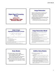
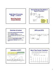
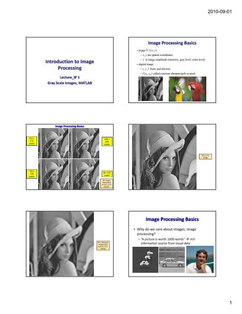
512 x<br />
512<br />
pixels<br />
128 x<br />
128<br />
pixels<br />
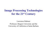
<strong>Introduction</strong> <strong>to</strong> <strong>Image</strong><br />
<strong>Processing</strong><br />
Lecture_IP 1<br />
Gray Scale <strong>Image</strong>s, MATLAB<br />
<strong>Image</strong> <strong>Processing</strong> <strong>Basics</strong><br />
256 x<br />
256<br />
pixels<br />
64 x 64<br />
pixels<br />
All images<br />
interpolated<br />
<strong>to</strong> 512 x 512<br />
format<br />
64 x 64image<br />
interpolated<br />
<strong>to</strong> 512 x 512<br />
format<br />
<strong>Image</strong> <strong>Processing</strong> <strong>Basics</strong><br />
iimage f( x, y)<br />
− xy , are spatial coordinates<br />
− f is image amplitude (intensity, gray level, color level)<br />
i digital image<br />
− xyf , y , f finite and discrete<br />
− f( x , y ) called a picture element (pel) or pixel<br />
0 0<br />
<strong>Image</strong> <strong>Processing</strong> <strong>Basics</strong><br />
• Why do we care about images, image<br />
processing?<br />
– “A picture is worth 1000 words” rich<br />
information source from visual data<br />
512 x 512<br />
image<br />
2010-09-01<br />
1
<strong>Image</strong> <strong>Processing</strong> <strong>Basics</strong><br />
• <strong>Image</strong> types:<br />
– natural pho<strong>to</strong>graphic images (jpg)<br />
– artistic and hand done drawings (pdf)<br />
– scientific images (satellite pho<strong>to</strong>s pho<strong>to</strong>s, medical images<br />
such as X‐rays and MRIs, cat scans, UV scans)<br />
– engineering drawings, technical specifications, etc.<br />
Why Digital <strong>Image</strong> <strong>Processing</strong><br />
• Lossless representations of images<br />
– no degradation and perfect reproduction<br />
– ability <strong>to</strong> duplicate without any loss of quality<br />
• Sophisticated and powerful digital signal processing<br />
algorithms l ith<br />
‐‐ Adobe Pho<strong>to</strong>shop; Pho<strong>to</strong>shop Elements<br />
‐‐ easy <strong>to</strong> process and manipulate images<br />
• Low cost of s<strong>to</strong>rage and transmission<br />
‐‐ modern compression methods can reduce s<strong>to</strong>rage rate by<br />
fac<strong>to</strong>rs of 30 or more with almost no loss of perceived quality<br />
‐‐ single CD can s<strong>to</strong>re thousands of pho<strong>to</strong>s<br />
Why Process <strong>Image</strong>s<br />
• Enhancement and Res<strong>to</strong>ration<br />
– removal of artifacts and scratches from old pho<strong>to</strong>s<br />
– improve contrast and lighting of existing pho<strong>to</strong>s<br />
– correct blurring due <strong>to</strong> motion in pho<strong>to</strong>s<br />
• Transmission and S<strong>to</strong>rage<br />
– compression for reduced s<strong>to</strong>rage and transmission costs (e.g., from<br />
outer space)<br />
– encoding for efficient transmission<br />
• <strong>Image</strong> Understanding<br />
– analysis and classification of image components<br />
– face recognition and classification<br />
– object identification (e.g., people, beach, sunset)<br />
• Security and Rights Protection<br />
– encryption and watermarking<br />
Processed <strong>Image</strong>s<br />
Famous processed image from World Trade Center<br />
9/11/2001<br />
<strong>Image</strong>s From Outer Space <strong>Image</strong>s From Outer Space<br />
2010-09-01<br />
2
Applications of Digital <strong>Image</strong> <strong>Processing</strong><br />
• Compression<br />
– standards‐based, JBIG, JPEG, JPEG2000<br />
• Manipulation and Res<strong>to</strong>ration<br />
– noise removal<br />
– noise reduction<br />
– morphing hi pairs i of f images i<br />
– res<strong>to</strong>ration of blurred and damaged images<br />
• Other<br />
– visual mosaicing and virtual views<br />
– face detection<br />
– visible and invisible watermarking<br />
– error concealment and resilience in transmission<br />
Original <strong>Image</strong> (8-bit<br />
gray scale)<br />
24 bit<br />
<strong>Image</strong> Quantization<br />
Original <strong>Image</strong> (5-bit<br />
gray scale)<br />
Original <strong>Image</strong> (2-bit<br />
gray scale)<br />
<strong>Image</strong> Compression<br />
Original <strong>Image</strong> (4-bit color<br />
scale, pseudo-color)<br />
1 bit<br />
0.5 bit 0.25 bit<br />
<strong>Image</strong>/Video Compression<br />
• Color image with 600x800 pixels<br />
– without compression each pixel needs 8 bits for red, green and<br />
blue components<br />
– <strong>to</strong>tal bit rate of 600*800*24 bits/pixel =1.44 megabytes<br />
– after JPEG compression can achieve almost lossless<br />
(perceptually) compression using 89 kilobytes giving a<br />
compression ratio of about 16:1<br />
• Movie with 720x480 pixels per frame, 30 frames/sec, 24<br />
bits/pixel (color frames)<br />
– without compression the <strong>to</strong>tal bit rate is 720x480x30x24=243<br />
megbits/second or 30 megabytes per second<br />
– with MPEG compression (for DVD) can compress video <strong>to</strong> about<br />
5 megabits/second or a compression ratio of about 48:1<br />
<strong>Image</strong> Compression<br />
8 bit 0.5 bit<br />
0.33 bit 0.25 bit<br />
<strong>Image</strong> Compression<br />
2010-09-01<br />
3
Examples of <strong>Image</strong> <strong>Processing</strong><br />
Enhancement, Denoising,<br />
Deblurring, Sampling Rate<br />
Conversion<br />
<strong>Image</strong> Denoising Denoising‐Median Median Filtering<br />
% Read in the image g and display p y it. % Add noise <strong>to</strong> the image. g<br />
% Filter the noisy y image g with an<br />
I = imread('eight.tif');<br />
imshow(I,'border','tight');<br />
J = imnoise(I,'salt & pepper',0.02);<br />
figure, imshow(J,'border','tight')<br />
averaging filter and display the<br />
results.<br />
K=filter2(fspecial('average',3),J)/255;<br />
figure, imshow(K,'border','tight')<br />
% Now use a median filter <strong>to</strong> filter the noisy image and display the<br />
% results. Notice that medfilt2 does a better job of removing noise,<br />
% with less blurring of edges.<br />
L = medfilt2(J,[3 3]);<br />
figure, imshow(L,'border','tight')<br />
<strong>Image</strong> Enhancement (enhance_image.m<br />
( enhance_image.m)<br />
% read and display dark image<br />
I=imread('pout.tif');<br />
imshow(I);<br />
% enhance contrast and<br />
display by computing image<br />
his<strong>to</strong>gram and equalizing<br />
his<strong>to</strong>gram levels<br />
figure,imhist(I);<br />
I2=histeq(I);<br />
% display enhanced image<br />
% display enhanced image<br />
his<strong>to</strong>gram<br />
figure,imshow(I2,'border','tight');<br />
figure,imhist(I2);<br />
<strong>Image</strong> Denoising Denoising‐Adaptive Adaptive Filtering<br />
(1) Original Saturn<br />
<strong>Image</strong> – Color <strong>Image</strong><br />
(3) Saturn <strong>Image</strong><br />
with Additive<br />
Gaussian Noise<br />
(1) (2) (3)<br />
(2) Gray Scale Saturn<br />
<strong>Image</strong><br />
(4) Noise Removed<br />
<strong>Image</strong> Using Wiener<br />
Filter<br />
<strong>Image</strong> Denoising <strong>Image</strong> Deblurring<br />
2010-09-01<br />
(4)<br />
4
<strong>Image</strong> Deblurring –Lucy Lucy‐Richardson Richardson Filter<br />
% Read an image in<strong>to</strong> the MATLAB<br />
workspace.; crop image<br />
I = imread('board.tif');<br />
I = I(50+[1:256],2+[1:256],:);<br />
figure;imshow(I,'border','tight');<br />
title('Original <strong>Image</strong>');<br />
% Use deconvlucy <strong>to</strong> res<strong>to</strong>re the blurred and<br />
noisy image<br />
luc1 = deconvlucy(BlurredNoisy,PSF,5);<br />
figure; imshow(luc1,'border','tight');<br />
% Create the PSF.<br />
PSF = fspecial('gaussian',5,5);<br />
% Create a simulated blur in the image and add noise.<br />
Blurred =imfilter(I,PSF,'symmetric','conv');<br />
V = .002;<br />
BlurredNoisy = imnoise(Blurred,'gaussian',0,V);<br />
figure;imshow(BlurredNoisy,'border','tight');<br />
title('Blurred and Noisy <strong>Image</strong>');<br />
Other <strong>Image</strong> <strong>Processing</strong> Effects<br />
Visual Mosaic, Watermarking, Error<br />
Concealment, Resampling<br />
Watermarks<br />
• A visible watermark is a visible translucent image which is<br />
overlaid on the primary image.<br />
• A watermark allows the primary image <strong>to</strong> be viewed, but still<br />
marks it clearly as the property of the owning organization.<br />
• It is important <strong>to</strong> overlay the watermark in a way which makes<br />
it difficult <strong>to</strong> remove, if the goal of indicating property rights is<br />
<strong>to</strong> be achieved.<br />
(a) Original <strong>Image</strong><br />
(c) Original <strong>Image</strong> Down-<br />
Sampled by 2:1, then Up-<br />
Sampled by 2:1<br />
(b) Original <strong>Image</strong><br />
Down-Sampled by 2:1<br />
<strong>Image</strong> Sampling<br />
Rate Changes<br />
Visual Mosaic<br />
Watermarks<br />
(d) Original <strong>Image</strong> Up-Sampled by 2:1<br />
2010-09-01<br />
(e) Original <strong>Image</strong><br />
Up-Sampled by<br />
2:1, then Down-<br />
Sampled by 2:1<br />
• An invisible watermark is an overlaid image which cannot be seen,<br />
but which can be detected algorithmically.<br />
• Different applications of this technology call for two very different<br />
types of invisible watermarks:<br />
– A watermark which is destroyed when the image is manipulated<br />
digitally in any way may be useful in proving authenticity of an image.<br />
If the watermark is still intact, intact then the image has not been<br />
"doc<strong>to</strong>red." If the watermark has been destroyed, then the image has<br />
been tampered with. Such a technology might be important, for<br />
example, in admitting digital images as evidence in court.<br />
– An invisible watermark which is very resistant <strong>to</strong> destruction under<br />
any image manipulation might be useful in verifying ownership of an<br />
image suspected of misappropriation. Digital detection of the<br />
watermark would indicate the source of the image.<br />
5
Visible Digital Watermarks<br />
Courtesy IBM Watson web page “Vatican<br />
Digital Library<br />
Invisible Watermark<br />
Upper right half of image invisibly<br />
watermarked, lower left half not<br />
watermarked.<br />
Upper pattern is watermark detected<br />
from upper right half of image; lower<br />
pattern is watermark detected from<br />
lower left half of image.<br />
Error Error Concealment Error Concealment<br />
Under Sampling of <strong>Image</strong><br />
Proper sampling of image Under sampling of image –note the Moire<br />
patterns due <strong>to</strong> image aliasing<br />
<strong>Image</strong> <strong>Processing</strong> <strong>Processing</strong> Using MATLAB<br />
2010-09-01<br />
6
Related Fields <strong>to</strong> <strong>Image</strong> <strong>Processing</strong><br />
• <strong>Image</strong> analysis<br />
– determine image properties (type of image<br />
(pho<strong>to</strong>, drawing, medical image)<br />
– determine image components (objects in image,<br />
scene ddescription) i ti )<br />
• Computer vision<br />
– analyze image <strong>to</strong> determine impediments <strong>to</strong><br />
motion of au<strong>to</strong>nomous vehicles<br />
– identify faces in images<br />
– identify fish in coral reef (Joe Wilder vision<br />
lecture)<br />
<strong>Image</strong> <strong>Processing</strong> Levels<br />
• Low Level <strong>Processing</strong> (input and output are images)<br />
– noise reduction – denoising of images<br />
– contrast enhancement –improve lighting for viewing images<br />
– image enhancement –sharpen image at edges or in points of maximal<br />
interest<br />
• Mid Level <strong>Processing</strong> (input is an image, output is a set of image attributes)<br />
‐‐ image segmentation (partition in<strong>to</strong> regions or objects); edge detection<br />
‐‐ object description (e.g., size, color, orientation)<br />
‐‐ object classification (recognition, e.g., faces)<br />
• High Level <strong>Processing</strong><br />
‐‐ making sense of ensemble of recognized objects (e.g., path planning,<br />
alerting, alarming)<br />
MATLAB <strong>Image</strong> <strong>Processing</strong> MATLAB <strong>Image</strong> <strong>Processing</strong> Fundamentals<br />
MATLAB <strong>Image</strong> <strong>Processing</strong><br />
⎡ f(0,0) f(0,1) ... f(0, N −1)<br />
⎤<br />
⎢<br />
f(1, 0) f(1,1) ... f(1, N −1)<br />
⎥<br />
f( x, y)<br />
= ⎢ ⎥<br />
⎢ ⎥<br />
⎢ ⎥<br />
⎣f( M,1) f( M,2) ... f( M −1, N −1)<br />
⎦<br />
⎡f(1,1) f(1,2) ... f(1,N) ⎤<br />
⎢<br />
f(2,1) f(2,2) ... f(2,N)<br />
⎥<br />
f= ⎢ ⎥<br />
⎢ ⎥<br />
⎢ ⎥<br />
⎣f(M,1) f(M,2) ... f(M,N) ⎦<br />
MATLAB <strong>Image</strong> Indexing<br />
Conventional <strong>Image</strong> Indexing<br />
f(1, 1) = f(0,0)<br />
f(M, N) = f(M-1,N-1)<br />
Equivalence of<br />
MATLAB and<br />
Conventional<br />
<strong>Image</strong> Indexing<br />
f( x, y) →M rows, N columns ⇒ M× N size image<br />
conventional indexing (0 : M − 1× 0 : N −1)<br />
MATLAB <strong>Image</strong>:<br />
f(r,c) ↔ (1: M,1: N)<br />
Conventional image<br />
coordinates<br />
MATLAB image<br />
coordinates<br />
<strong>Image</strong> Formats for MATLAB<br />
2010-09-01<br />
7
<strong>Image</strong> IO in MATLAB<br />
• <strong>Image</strong> read command:<br />
– f = imread(‘filename’); % f = imread(‘lena.tif’);<br />
– [M,N] = size(f); % M=512, N=512, ; pixels‐8 bits<br />
• I<strong>Image</strong> di display l command: d<br />
‐‐ imshow(f, [low, high]); % display as black image<br />
intensity at or below low; display as white image<br />
intensity at or above high;<br />
‐‐ imshow(f, [ ]); % expands dynamic range so that<br />
max=white, min=black<br />
‐‐ impixelinfo; % uses cursor <strong>to</strong> read image<br />
coordinates and pixel intensity values<br />
f = imread(‘saturn.tif’);<br />
[M,N] = size(f); % M=328, N=448<br />
imshow(f);<br />
M=size(f,1); number of rows in f<br />
N=size(f,2); number of columns in f<br />
Example<br />
Example<br />
imshow(f, [64,128]);<br />
• f=[255 230 180; 155 130 105; 80 50 0];<br />
• imshow(f,[ ],’InitialMagnification’,’fit’);<br />
f=imread(‘lena.tif’);<br />
whos<br />
name: f<br />
size: 512 x 512<br />
bytes: 262144<br />
class: uint8<br />
imshow(f);<br />
Example<br />
Full path read: f=imread(‘C:\data\matlab\image files\lena.tif’);<br />
Overview<br />
f=imread(‘rose.tif’);<br />
im<strong>to</strong>ol(f);<br />
Example<br />
<strong>Image</strong> Tool<br />
Pixel Value<br />
Cropped <strong>Image</strong><br />
Pixel Region g<br />
2010-09-01<br />
8
<strong>Image</strong> Tool<br />
im<strong>to</strong>ol is extremely useful <strong>to</strong>ol for gaining an<br />
understanding of image properties<br />
<strong>Image</strong> IO IO in MATLAB MATLAB<br />
• <strong>Image</strong> write command:<br />
– imwrite(f, ’filename’); % writes <strong>to</strong> filename (must have valid<br />
extension)<br />
– imwrite(f,’filename’,’tif’); % writes <strong>to</strong> filename.tif<br />
– imwrite(f, ’filename.jpg’, ’quality’, q); % 0 ≤q≤100<br />
• File size information:<br />
– imfinfo filename; imfinfo(‘filename’);<br />
– K=imfinfo(‘filename’); % K is structure variable<br />
– K.Height, K.Width;<br />
• Export figure images <strong>to</strong> disk:<br />
– print –fno –dfileformat –rresno filename; % no is figure number;<br />
fileformat from list; resno=dpi resolution of file<br />
– print ‐f1 –dtiff –r300 saturn_clip.tif; % save figure 1, in tiff format,<br />
using 300 dpi resolution, <strong>to</strong> filename ‘saturn_clip.tif’<br />
<strong>Image</strong> Tool<br />
pseudo-color with<br />
colormap l set tt <strong>to</strong> ‘hot’; ‘ht’ filename:’rose_hot.jpg’<br />
Example ‐ imfinfo imfinfo(‘saturn.tif’);<br />
(‘saturn.tif’);<br />
Filename: 'saturn.tif'<br />
FileModDate: '07‐Jul‐2004 15:31:54'<br />
FileSize: 144184<br />
Format: 'tif'<br />
FormatVersion: []<br />
Width: 438<br />
Height: 328<br />
BitD BitDepth: th 8<br />
ColorType: 'grayscale'<br />
FormatSignature: [73 73 42 0]<br />
ByteOrder: 'little‐endian'<br />
NewSubFileType: 0<br />
BitsPerSample: 8<br />
Compression: 'Uncompressed'<br />
Pho<strong>to</strong>metricInterpretation: 'BlackIsZero'<br />
StripOffsets: [19x1 double]<br />
SamplesPerPixel: 1<br />
RowsPerStrip: 18<br />
Example Example<br />
StripByteCounts: [19x1 double]<br />
XResolution: 72<br />
YResolution: 72<br />
ResolutionUnit: 'Inch'<br />
Colormap: []<br />
PlanarConfiguration: 'Chunky'<br />
TileWidth: []<br />
TileLength: []<br />
TileOffsets: []<br />
TileByteCounts: []<br />
Orientation: 1<br />
FillOrder: 1<br />
GrayResponseUnit: 0.0100<br />
MaxSampleValue: 255<br />
MinSampleValue: 0<br />
Thresholding: 1<br />
<strong>Image</strong>Description: [1x168 char]<br />
2010-09-01<br />
9
<strong>Image</strong> Size<br />
• f=imread(‘circuitboard.tif’);<br />
• imwrite(f,’circuitboard_r300.tif’,’compre<br />
ssion’,’none’,’resolution’,[300 300]);<br />
• K=imfinfo(‘circuitboard_r300.tif’);<br />
• K.XResolution=300; K.YResolution=300;<br />
1.5 x 1.5 inches<br />
• imwrite(f,’circuitboard_r200.tif’,’compre<br />
ssion’,’none’,’resolution’,[200 200]);<br />
• K=imfinfo(‘circuitboard_r200.tif’);<br />
• K.XResolution=200; K.YResolution=200;<br />
2.25 x 225 inches<br />
<strong>Image</strong> Data Classes<br />
• f=imread(‘lena.tif’);<br />
• whos<br />
– Name Size Bytes Class Attributes<br />
– f 512x512 262144 uint8<br />
• max (f(:))=245; min(f(:))=24;<br />
• g=double(f);<br />
• whos<br />
– Name Size Bytes Class Attributes<br />
– f 512x512 262144 uint8<br />
– g 512x512 2097152 double<br />
• max(g(:))=245; min(g(:))=24;<br />
<strong>Image</strong> Types<br />
• Intensity images ‐ generally gray scale images<br />
whose values represent image intensity; class can be<br />
double (floating point), uint8 (integers from 0 <strong>to</strong><br />
255), uint16 (integers from 0 <strong>to</strong> 65535) or scaled<br />
double in the range [0,1]<br />
• Binary inary images images ‐ logical array of 0s and 1s; s; obtained<br />
using function logical on a numeric array of ones and<br />
zeros (half<strong>to</strong>ne)<br />
• Indexed images ‐ image with two components,<br />
namely a data matrix of integers, X, and a color map<br />
matrix, map.<br />
• RGB images ‐ image with 3 complementary color sets<br />
of intensity<br />
<strong>Image</strong> Data Classes<br />
Data classes double through single are numeric data classes;<br />
Data class char is a character class and data class logical is a<br />
logical class.<br />
<strong>Image</strong> Data Classes<br />
• All numeric computations in MATLAB are<br />
done using using double double quantities<br />
• Data class uint8 is mostly used for reading and<br />
s<strong>to</strong>ring t i iimages as 88‐bit bit images i<br />
• Data class double requires 8 bytes per<br />
number; data class uint8 requires 1 byte per<br />
number<br />
<strong>Image</strong> Types<br />
• <strong>to</strong> convert from gray‐scale image <strong>to</strong> binary<br />
image:<br />
– f=imread(‘image.tif’);<br />
g=f;<br />
– g=f;<br />
– g(find(f >= 128))=1;<br />
– g(find(f < 128))=0;<br />
– b=logical(g);<br />
– islogical(b)<br />
1<br />
2010-09-01<br />
10
f, Gray<br />
Scale<br />
<strong>Image</strong>,<br />
uint8<br />
[0 255]<br />
<strong>Image</strong> Types<br />
lena.tif (512 x 512 x 8 bits) lena_binary.tif (512 x 512 x 1 bits)<br />
g=mat2gray(f)<br />
<strong>Image</strong> Conversions<br />
g, Gray<br />
Scale<br />
<strong>Image</strong>,<br />
double<br />
[0 1] <strong>Image</strong><br />
<strong>Processing</strong><br />
h, Gray<br />
Scale<br />
<strong>Image</strong>,<br />
double<br />
[0 1]<br />
p=im2uint8(f)<br />
p, Gray<br />
Scale<br />
<strong>Image</strong>,<br />
uint8<br />
[0 255]<br />
<strong>Image</strong> Conversions –im2uint8 im2uint8<br />
im2uint8 scales an image in the range [0 1] <strong>to</strong> an<br />
image in the range [0 255] by scaling the image<br />
values by 255 and clipping below 0 and above 255<br />
• f = [‐0.5 [ 0505;0 0.5; 0.75 51.5]; 5];<br />
• g = im2uint8(f); What is g?<br />
g=[0 128; 191 255];<br />
f11; % 1.5 goes <strong>to</strong> 255<br />
scale by 255; 0.5 goes <strong>to</strong> 128, 0.75 goes <strong>to</strong> 191<br />
<strong>Image</strong> Conversions<br />
• <strong>Image</strong>s classified according <strong>to</strong> both class_image<br />
(double, uint8, …) and type_image (intensity, binary,<br />
indexed, RGB)<br />
• Can readily convert between data classes and image<br />
types, e.g.,<br />
– Data class conversions: B = class_name(A);<br />
– A: class uint8 image<br />
– B = double(A) converts from uint8 <strong>to</strong> double<br />
– C: class double image<br />
– D = uint8(C) converts from double [0 255] <strong>to</strong> uint8 (integers<br />
in [0 255]); uint8 truncates below 0 and above 255<br />
– g = im2uint8(f) scales f <strong>to</strong> [0 255] then converts <strong>to</strong> integer<br />
values<br />
<strong>Image</strong> Conversions<br />
• uint8: converts double <strong>to</strong> integers in<br />
range of [0 255]<br />
• im2uint8: scales by 255 and integerizes <strong>to</strong><br />
range [0 255]<br />
• mat2gray: scale <strong>to</strong> range [0 1]<br />
• im2double: convert <strong>to</strong> double precision<br />
<strong>Image</strong> Conversions – im2double<br />
• im2double converts input <strong>to</strong> class double<br />
– if input of class uint8, uint16 or logical, im2double<br />
converts <strong>to</strong> class double with values in range [0 1]<br />
– if input of class single or double, double im2double<br />
returns array of class double, but numerically<br />
equal <strong>to</strong> the input<br />
– mat2gray can be used <strong>to</strong> convert an array of any<br />
class <strong>to</strong> a double array with values in range [0 1]<br />
2010-09-01<br />
11
<strong>Image</strong> Conversions – im2double<br />
• Example:<br />
– h = uint8([25 50; 128 200]);<br />
– g = im2double(h);<br />
– g g=[0.0980 [0 0980 00.1961;0.5020 1961;0 5020 00.7843]; 7843]; % converts<br />
integers <strong>to</strong> double precision values in range [0 1];<br />
<strong>Image</strong> Conversion Examples –mat2gray mat2gray<br />
• h = uint8([25 50; 128 200]);<br />
• g = mat2gray(h); % what is g?<br />
g = [0 0.1429; 0.5886 1]; Amin=25; Amax=200<br />
25 0; 50 (50‐25)/175=0.1429;<br />
128 (128‐25)/175=0.5886; 200 (200‐25)/175=1<br />
• g = im2bw(f,T); % produces a binary image, g,<br />
from intensity image, f, by thresholding such<br />
that all pixels < T go <strong>to</strong> 0, all others go <strong>to</strong> 1<br />
<strong>Image</strong> Conversion Examples –im2bw im2bw<br />
• im2bw performs conversion <strong>to</strong> class logical<br />
where nonzero elements are converted <strong>to</strong> 1s<br />
and zero elements are converted <strong>to</strong> 0s in the<br />
output<br />
• equivalently l l we could ld ddo the h following: f ll<br />
‐ g = f > T; % where T is the threshold for conversion<br />
<strong>to</strong> 1s and below T inputs converted <strong>to</strong> 0s<br />
‐ g = im2bw(f, T); performs same operations as<br />
above; threshold T must be in range [0 1]; for uint8<br />
input, threshold is T*255<br />
<strong>Image</strong> Conversions –mat2gray mat2gray<br />
• mat2gray converts image of any class <strong>to</strong> array<br />
of class double scaled <strong>to</strong> the range [0 1]<br />
• calling sequence is:<br />
– g = mat2gray(A, t2 (A [A [Amin, i A Amax]); ]) % g has h values l iin<br />
range 0 (black) <strong>to</strong> 1 (white) with clipping below<br />
Amin and above Amax; Amin and Amax need not<br />
be specified –routine finds min and max prior <strong>to</strong><br />
conversion and treats them as Amin and Amax<br />
f=imread(‘lena.tif’);<br />
figure,imshow(f);<br />
max(f(:))=245;<br />
min(f(:))=24;<br />
Simple Example<br />
f1=mat2gray(f);<br />
f2=im2uint8(f1);<br />
figure,imshow(f2);<br />
max(f2(:))=255;<br />
min(f2(:))=0;<br />
<strong>Image</strong> Conversion Examples<br />
• f=[1 2; 3 4];<br />
• convert <strong>to</strong> binary such that values 1 and 2 become 0 and the<br />
other two values become 1<br />
– first convert <strong>to</strong> range [0 1]<br />
– g = mat2gray(f) ; g= [0 0.3333; 0.6667 1.0];<br />
– next convert <strong>to</strong> binary using threshold of 0.6<br />
– gb = im2bw(g, 0.6); gb= [0 0; 1 1]<br />
• alternatively can use<br />
– gb = f > 2; gb=[0 0; 1 1]<br />
• convert gb <strong>to</strong> numerical array of 0s and 1s:<br />
– gbd = im2double(gb); gbd=[0 0; 1 1]<br />
• gbd=im2double(im2bw(mat2gray(f), 0.6));<br />
• gbd = double(f > 2);<br />
2010-09-01<br />
12
<strong>Image</strong> Conversion Examples<br />
⎡25 50 ⎤ ⎡ 0.5 0.75⎤<br />
f1 = ⎢ (double) g1<br />
(double)<br />
75 100<br />
⎥ = ⎢<br />
0.85 0.99<br />
⎥<br />
⎣ ⎦ ⎣ ⎦<br />
⎡25 50 ⎤<br />
f2= uint8( f1)<br />
= ⎢<br />
75 100<br />
⎥<br />
⎣ ⎦<br />
⎡1 1⎤<br />
g2= uint8( g1)<br />
= ⎢ (integerize <strong>to</strong> [0 255] range)<br />
1 1<br />
⎥<br />
⎣ ⎦<br />
⎡ 255<br />
f3= im2uint8( f1)<br />
= ⎢<br />
⎣255 255 ⎤<br />
255<br />
⎥<br />
⎦<br />
⎡ 128<br />
g3= im2uint8( g1)<br />
= ⎢<br />
⎣217 191 ⎤<br />
(scale by 255 and integerize)<br />
252<br />
⎥<br />
⎦<br />
⎡ 0<br />
f4= mat2gray( f1)<br />
= ⎢<br />
⎣0.66 0.33⎤<br />
⎡ 0<br />
1<br />
⎥ g4= mat2gray( g1)<br />
= ⎢<br />
⎦<br />
⎣0.71 0.51⎤<br />
(scale <strong>to</strong> [0 1] range)<br />
1<br />
⎥<br />
⎦<br />
⎡25 50 ⎤<br />
f5= im2double( f1)<br />
= ⎢<br />
75 100<br />
⎥<br />
⎣ ⎦<br />
⎡ 0.5 0.75⎤<br />
g5= im2double( g1)<br />
= ⎢ (convert <strong>to</strong> double)<br />
0.85 0.99<br />
⎥<br />
⎣ ⎦<br />
<strong>Image</strong> Conversion Examples<br />
original lena.tif image<br />
f = imread(‘lena.tif’); %<br />
image is 512 x 512 gray<br />
scale image (8 bits/pixel)<br />
<strong>Image</strong> Conversion Examples<br />
hnd = im2bw(g); %<br />
convert <strong>to</strong> black-andwhite<br />
image without<br />
dithering<br />
<strong>Image</strong> Conversion Examples<br />
⎡25 f 1 = ⎢<br />
⎣75 50 ⎤<br />
(uint8)<br />
100<br />
⎥<br />
⎦<br />
⎡25 f2= uint8( f1)<br />
= ⎢<br />
⎣75 50 ⎤<br />
100<br />
⎥<br />
⎦<br />
⎡ 255<br />
f3= im2uint8( f1)<br />
= ⎢<br />
⎣255 255 ⎤<br />
255<br />
⎥<br />
⎦<br />
⎡ 0<br />
f4= mat2gray( f1)<br />
= ⎢<br />
⎣0.66 0.33⎤<br />
1<br />
⎥<br />
⎦<br />
⎡25 50 ⎤<br />
f5= im2double( f1)<br />
= ⎢<br />
75 100<br />
⎥<br />
⎣ ⎦<br />
<strong>Image</strong> Conversion Examples<br />
f = imread(‘lena.tif’); %<br />
image is 512 x 512 gray<br />
scale image (8 bits/pixel)<br />
g = mat2gray(f); %<br />
convert scale from [0 [ 255] ]<br />
<strong>to</strong> [0 1]<br />
h = dither(g); % convert <strong>to</strong><br />
black-and-white image<br />
using dithering, 512 x 512<br />
bits<br />
<strong>Image</strong> Conversion Examples<br />
2010-09-01<br />
13
<strong>Image</strong> Conversion Examples <strong>Image</strong> Conversion Examples<br />
Array Indexing<br />
• V = [1 3 5 7 9]; % 1 row, 5 columns<br />
• V’ = V(:) = [1; 3; 5; 7; 9]; % 5 rows, 1 column<br />
• V(1:3) = [1 3 5]; % 1 row, 3 columns<br />
• V(3:end) = [5 7 9]; % 1 row row, 3 columns<br />
• V(end:‐2:1) = [9 5 1]; % 1 row, 3 columns<br />
• V([1 4 5]) = [1 7 9]; % 1 row, 3 columns<br />
• V = linspace(a,b,n); generates row vec<strong>to</strong>r beginning<br />
at a, ending at b, with n equi‐spaced elements<br />
• V = linspace(1,9,5) = [1 3 5 7 9]; % 1 row, 5 columns<br />
Matrix Matrix Operations – matrix sums<br />
• matrix sums (3 possible ways of computing)<br />
– A = [1 2 3; 4 5 6; 7 8 9]; % 3 rows, 3 columns<br />
– col_sums = sum(A); % col_sums=[12 15 18]<br />
– <strong>to</strong>tal_sum = sum(col_sums); % <strong>to</strong>tal_sum=45<br />
– <strong>to</strong>tal_sum1 = sum(A(:)); % <strong>to</strong>tal_sum1=45;<br />
– <strong>to</strong>tal_sum2 = sum(sum(A)); % <strong>to</strong>tal_sum2=45<br />
Matrix Indexing<br />
• A = [1 2 3; 4 5 6; 7 8 9]; % 3 rows, 3 columns<br />
• A(2, 3) = 6; % second row, third column entry<br />
• A(:, 3) = [3; 6; 9]; % third column, all entries<br />
• A(2, :) = [4 5 6]; % second row, all entries<br />
• A(1:2, 1:3) = [1 2 3; 4 5 6]; % first and second rows, all three<br />
columns<br />
• A(end, end) = 9; % last entry in matrix<br />
• A(end, end –2)=7; % entry in end row, end column ‐2<br />
• A(2:end, end:‐2:1) = [6 4; 9 7]; rows 2‐3, columns 3 and 1<br />
(backwards)<br />
• A([1 3], [2 3]) = [2 3;8 9]; % rows 1 and 3, columns 2 and 3<br />
• A(:)=[1; 4; 7; 2; 5; 8; 3; 6; 9]; % columns concatenated<br />
Max Opera<strong>to</strong>r<br />
• C = max(A); % C = row vec<strong>to</strong>r with max of each<br />
column<br />
• C = max(A, B); % C = array of largest elements of<br />
A or B<br />
• C = max(A, [ ], dim); % C has the largest<br />
elements along dimension of A specified by<br />
scalar dim<br />
• [C, I] = max(A); % C is a row vec<strong>to</strong>r with max of<br />
each column, and I is a row vec<strong>to</strong>r with row index<br />
for each column max<br />
2010-09-01<br />
14
Max Opera<strong>to</strong>r Examples<br />
• A = [1 4 7;2 5 8; 3 6 9]; B = [9 6 3;8 5 2; 7 4 1];<br />
• C = max(A) = [3 6 9]; % maximum of each column<br />
• C = max(A, B) = [9 6 7; 8 5 8; 7 6 9]; % largest<br />
elements of A or B at each row and column index<br />
• C = max(A max(A, [ ], ] 2) = [7; 8; 9]; % largest elements<br />
along dimension of A specified by last argument<br />
(2=rows, 1=columns)<br />
• C= max(A, [ ], 1) = [3 6 9];<br />
• [C, I] = max(A)=max(A, [ ], 1); C = [3 6 9]; I = [3 3 3]; %<br />
I = indices of maximums<br />
• [C, I]=max(A, [ ], 2); C=[7; 8; 9], I=[3 3 3];<br />
Matrix Operations – linear indexing<br />
• MATLAB functions sub2ind and ind2sub<br />
convert back and forth between row‐column<br />
subscripts and linear indices<br />
‐ linear_indices = sub2ind(size(H), r, c); % r is the<br />
row index (or array of indices), indices) c is the column<br />
index (or array of indices)<br />
- linear_indices = sub2ind([4 4],[1 2 4], [3 4 3]);<br />
% linear_indices = [9 14 12];<br />
‐ [r, c] = ind2sub(size(H), linear_indices);<br />
- [r, c]=ind2sub([4 4], [9 14 12]);<br />
% r=[1 2 4], c=[3 4 3]<br />
Standard MATLAB Arrays<br />
• zeros(M, N) – generates an M row, N column array of<br />
0s of class double<br />
• ones(M, N) – generates an M row, N column array<br />
of 1s of class double<br />
• rand(M, d( N) ) – generates an M row, N column l array<br />
whose entries are uniformly distributed random<br />
numbers in the interval [0 1]<br />
• randn(M, N) – generates an M row, N column array<br />
whose numbers are normally distributed (i.e.,<br />
Gaussian) random numbers with mean 0 and<br />
variance 1<br />
Matrix Operations – linear indexing<br />
• use a single subscript <strong>to</strong> index a matrix<br />
• example:<br />
⎡ 1 0.5 0.3333 0.25 ⎤<br />
⎢<br />
0.5 0.3333 0.25 0.2<br />
⎥<br />
H= ⎢ ⎥<br />
⎢0.3333 0.25 0.2 0.1667⎥<br />
⎢ ⎥<br />
⎣ 00.25 25 00.2 2 00.1667 1667 00.1429 1429 ⎦<br />
• H([2 11]); % H=[0.5 0.2] –extracts 2nd and 11th elements of H; elements counted by columns<br />
• extract values of H at (1,3), (2,4) and (4,3) –we do<br />
this by extracting row and column indices of the three<br />
pixels, i.e., (1,3) maps <strong>to</strong> 9; (2,4) maps <strong>to</strong> 14; (4,3)<br />
maps <strong>to</strong> 12<br />
f = imread(‘rose.tif’);<br />
imshow(f);<br />
Matrix Indexing Example<br />
fp=f(end:‐1:1,:);<br />
flip vertically<br />
(c) - fc=f(257:768,257:768);<br />
% image section<br />
(d) – fs=f(1:2:end,1:2:end);<br />
% subsampled image<br />
(e) = plot(f(512,:)); horizontal<br />
% scan line<br />
Standard MATLAB Arrays Arrays<br />
• A = 5*ones(3, 3); % A=[5 5 5;5 5 5; 5 5 5]<br />
• B = randn(1, 5000); hist(B, 100);<br />
2010-09-01<br />
15
Array and Matrix Arithmetic Opera<strong>to</strong>rs<br />
MATLAB m function<br />
• write MATLAB function that blends two input images in equal<br />
weight<br />
function [w, wmax, wmin]=imblend(f, g)<br />
% w is a blend of f and g with wmax and wmin the maximum and<br />
minimum values of the blend<br />
w1 = 0.5 * f;<br />
w2 = 0.5 * g;<br />
w = w1 + w2;<br />
wmax = max (w(:));<br />
wmin = min(w(:));<br />
f = [1 2; 3 4]; g = [1 2; 2 1];<br />
[w, wmax, wmin] = imblend(f, g);<br />
w=[1 2; 2.5 2.5];<br />
wmax=2.5;<br />
wmin=1;<br />
% could use w = 0.5 * (f + g); % however when (f + g) exceeds<br />
255 (for a uint8 array) the sum saturates and we get a wrong<br />
result<br />
Array and Matrix Arithmetic<br />
Opera<strong>to</strong>rs for <strong>Image</strong>s (uint8 arrays)<br />
Array and Matrix Arithmetic Opera<strong>to</strong>rs<br />
⎡a1 A= ⎢<br />
⎣a3 a2⎤ ,<br />
a4 ⎥<br />
⎦<br />
⎡b1 B= ⎢<br />
⎣b3 b2⎤<br />
b4<br />
⎥<br />
⎦<br />
i The array product of A and B is:<br />
⎡ ⎡a 11 b<br />
A.*B = ⎢<br />
⎣ab 33<br />
a 2 2b b 2 ⎤<br />
ab 44<br />
⎥<br />
⎦<br />
i whereas the matrix product yields the familiar result:<br />
⎡ab 11+ a2b3ab 12+ a2b4⎤ A*B= ⎢<br />
ab 31+ ab 43 ab 32+ ab 44<br />
⎥<br />
⎣ ⎦<br />
MATLAB m function<br />
• <strong>to</strong> alleviate the saturation problem use<br />
MATLAB function<br />
g = imlincomb(k1, f1, k2, f2)<br />
k1 = weight for f1;<br />
f1 = image 1;<br />
k2 = weight for f2;<br />
f2 = image 2;<br />
w = imlincomb(0.5, f, 0.5 g); % this no<br />
longer saturates on uint8 arrays<br />
MATLAB Relational and Logical Opera<strong>to</strong>rs<br />
A == B; 1 when A(i,j) = B(i,j), 0 otherwise<br />
A ~= B; 1 when A(i,j) ≠ B(i,j), 0 otherwise<br />
A >= B; 1 when A(i,j) ≥ B(i,j), 0 otherwise<br />
A = B = [1 1 0;1 1 1];<br />
A
MATLAB Relational Examples<br />
• A = [1 2 3; 4 5 6; 7 8 9];<br />
• B = [0 2 4; 3 5 6; 3 4 9];<br />
• A == B; [0 1 0; 0 1 1; 0 0 1];<br />
• A >= B; [1 1 0; 1 1 1; 1 1 1];<br />
• C = [1 2 0; 0 4 5];<br />
• D = [1 ‐2 3; 0 1 1];<br />
• C & D; [1 1 0; 0 1 1];<br />
• C | D; [1 1 1; 0 1 1];<br />
<strong>Image</strong> 1 – <strong>Image</strong> 2; tendency <strong>to</strong><br />
blacks (intensities near 0)<br />
<strong>Image</strong> Subtraction<br />
<strong>Image</strong> 1 – <strong>Image</strong> 2; his<strong>to</strong>gram<br />
equalized; improved brightness and<br />
contrast (still dark image)<br />
MATLAB Function, fgprod<br />
Product of two images; again there is<br />
a tendency <strong>to</strong> black as the product of<br />
two numbers (both
MATLAB Flow Control ‐ Switch<br />
switch switch_expression<br />
case case_expression<br />
statement(s)<br />
case {case_expression1, case_expression2, …}<br />
statement(s)<br />
otherwise<br />
statement(s)<br />
end<br />
switch newclass<br />
case ‘uint8’<br />
g = im2uint8(f);<br />
case ‘uint16’<br />
g = im2uint16(f);<br />
case ‘double’<br />
g = im2double(f);<br />
otherwise<br />
error(‘Unknown or improper image class.’);<br />
end<br />
Vec<strong>to</strong>rizing Loops –Example Example 1<br />
f(x) = Asin(x / 2π), x = 0,1,2,...,M-1<br />
For loop implementation:<br />
A =10;<br />
for x =1:M % Array indices in MATLAB cannot be 0<br />
f(x) = A * sin((x -1) / (2* pi));<br />
end<br />
Vec<strong>to</strong>rized MATLAB code :<br />
A =10;<br />
tpi = 2* pi;<br />
Ratio of time for loop versus<br />
vec<strong>to</strong>rized MATLAB code: 1.8<br />
x = 0 :M-1;<br />
f = A * sin(x / tpi);<br />
Vec<strong>to</strong>rizing Loops –Example Example 2<br />
Vec<strong>to</strong>rize function using meshgrid<br />
i [C, R] = meshgrid(c, r);<br />
i c, r vec<strong>to</strong>rs of horizontal (column) and<br />
vertical (row) coordinates<br />
i meshgrid transforms coordinate vec<strong>to</strong>rs<br />
in<strong>to</strong> arrays C and R that can be used <strong>to</strong><br />
compute function of two variables<br />
Example : want <strong>to</strong> evaluate function z= x+ y for<br />
integer values of x ranging from 1 <strong>to</strong> 3, and for<br />
integer values of y ranging from 10 <strong>to</strong> 14<br />
[X, Y] = meshgrid(1: 3, 10 :14);<br />
X = [1 2 3; 1 2 3; 1 2 3; 1 2 3; 1 2 3];<br />
Y = [10 10 10; 11 11 11; 12 12 12; 13 13 13; 14 14 14];<br />
Z = X + Y = [11 12 13; 12 13 14; 13 14 15; 14 15 16; 15 16 17];<br />
MATLAB Timing<br />
• tic; % sets variable tic <strong>to</strong> current clock time<br />
• run MATLAB code <strong>to</strong> be timed<br />
• <strong>to</strong>c; –Elapsed time is 0.xxx seconds<br />
• for timing function calls can use special<br />
function s=timeit(f) where f is the function<br />
handle for the function <strong>to</strong> be timed, and s is<br />
the measurement time, in seconds (timeit<br />
must be retrieved from course website)<br />
Vec<strong>to</strong>rizing Loops –Example Example 2<br />
Create MATLAB function <strong>to</strong> create a synthetic image<br />
of the form :<br />
f( x, y) = Asin( u0x+ v0y) First version uses nested "for" loops<br />
function f = twodsin1(A, u0, v0, M, N)<br />
f = zeros(M, N); % pre - allocation of memory<br />
for c = 1:N<br />
v0y = v0 * (c -1);<br />
for r = 1:M<br />
u0x = u0 * (r - 1);<br />
f(r, c) = A * sin(u0x + v0y);<br />
end<br />
end<br />
Time this version:<br />
f = twodsin1(1, 1/ (4 *pi), 1/ (4 * pi), 512, 512);<br />
imshow(f, [ ]);<br />
Time: 0.0215 seconds<br />
Vec<strong>to</strong>rizing Loops –Example Example 2<br />
Rewrite 2 -D sine function without loops<br />
function f = twodsin2(A, u0, v0, M, N)<br />
r = 0 :M - 1; % row coordinates<br />
c = 0 0:N :N - 1; % column coordinates<br />
[C, R] = meshgrid(c, r);<br />
f = A * sin(u0 *R + v0 * C);<br />
Time: 0.0157 seconds<br />
Ratio of times: 1.369<br />
2010-09-01<br />
18
Interactive IO<br />
• disp(argument) –display on screen<br />
• A = [1 2;3 4]; disp(A);<br />
1 2<br />
3 4<br />
• sc = ‘text string’; disp(sc);<br />
‘text text string’ string<br />
• t = input(‘message:’, ’s’) – accept screen input<br />
n = input(‘specify value for n:’);<br />
t = input(‘specify value for n:’,’s’); n=str2num(t);<br />
• [a,b,c,…] = strread(cstr, ’format’, ’param’, ’value’);<br />
• format = %f (floating point), %q(character strings), %d (integer)<br />
t = ’12.6, x2y, z’; [a,b,c] = strread(t, ’%f%q%q’, ’delimiter’, ’,’);<br />
a = 12.6; b = ‘x2y’, c = ‘z’ (b and c are cells); convert cells <strong>to</strong> character array<br />
d = char(b) = x2y, e = char(c) = z<br />
Cell Arrays and Structures<br />
• Cell array – multidimensional array whose elements are<br />
copies of other arrays – signaled by { and } brackets<br />
c = {‘gauss’, [1 0; 0 1], 3};<br />
c{1} = gauss (a character string)<br />
c{2} = [1 0; 0 1] ( a 2 x 2 matrix)<br />
c{3} = 3 ( a scalar)<br />
• Structure – grouping of a collection of dissimilar data in<strong>to</strong> a<br />
single variable –elements of structures addressed by fields<br />
S=structure ‐‐ enter elements of S via simple commands, e.g.,<br />
S.char_string = ‘gauss’;<br />
S.matrix = [1 0; 0 1];<br />
S.scalar = 3;<br />
MATLAB MATLAB <strong>Image</strong> <strong>Processing</strong><br />
Commands<br />
• K = imfinfo filename; % get file information in structure K<br />
– image_bytes = K.Width*K.Heights*K.Depth/8;<br />
• g = im2uint8(f); % convert from image <strong>to</strong> uint8<br />
‐ f ≤ 0 => 0; f ≥ 1 => 1; scale by 255 and round<br />
• g = mat2gray(A, [Amin Amax]); % converts double [ ] <strong>to</strong><br />
double [0 1]<br />
• g = im2double(f); % converts image of uint8 or double <strong>to</strong><br />
double<br />
‐ g = im2double(mat2gray(f)); % converts <strong>to</strong> [0 1] range<br />
String Compare<br />
• We assume that parameter param can have two forms, namely ‘norm1’ ([0 1]) or<br />
‘norm255’ ([0 255])<br />
• Use strcmp <strong>to</strong> decide which option <strong>to</strong> use<br />
f is image input<br />
f = double(f); % floating point values<br />
f = f‐min(f(:)); f min(f(:)); % min(f) set <strong>to</strong> 0<br />
f = f./max(f(:)); % max(f) set <strong>to</strong> 1<br />
if (strcmp(param, ’norm1’)<br />
g = f;<br />
elseif strcmp(param, ’norm255’)<br />
g = 255*f;<br />
else<br />
error(‘Unknown value of param.’);<br />
end<br />
MATLAB <strong>Image</strong> <strong>Processing</strong><br />
Commands<br />
• f = imread(‘filename’); % reads in file <strong>to</strong> array<br />
• imshow(f); % displays array as image, [0 255]<br />
‐ imshow(f, [low high]); % f(i,j) ≤ low => low (black)<br />
‐ % f(i,j) ≥ high => high (white)<br />
‐ imshow(f, [ ]); % low = min(min(f)); high = max(max(f));<br />
• pixval; % displays intensity values of pixels<br />
• imwrite(f, ’filename’); % writes image <strong>to</strong> disk<br />
‐ imwrite(f, ‘filename’, ‘tif’);<br />
‐ imwrite(f, ‘filename.jpg’, ‘quality’, q); % q in [0 100] range<br />
<strong>Image</strong>s on Website<br />
blood1.tif; 265<br />
rows, 272 columns,<br />
min=46, max=255<br />
breast.tif; 570<br />
rows, 482 columns,<br />
min=21, max=255<br />
building.tif; 240<br />
rows, 320 columns,<br />
min=21, max=255<br />
chalk.tif; 1040 rows,<br />
1040 columns,<br />
min=0, max=255<br />
checker.tif; 512<br />
rows, 512 columns,<br />
min=0, max=255<br />
circuitboard.tif; 450<br />
rows, 450 columns,<br />
min=0, max=255<br />
FTspectrum.tif; 257<br />
rows, 257 columns,<br />
min=0, max=255<br />
hardware.tif; 240<br />
rows, 320 columns,<br />
min=4, max=248<br />
2010-09-01<br />
19
<strong>Image</strong>s on Website<br />
iris.tif; 600 rows,<br />
600 columns,<br />
min=0, max=255<br />
iris_gray.tif; 600<br />
rows, 600 columns,<br />
min=27 min=27, max=255<br />
iris_luminence.tif;<br />
600 rows, 600<br />
columns, min=22,<br />
max=255<br />
lena.gif; 512 rows,<br />
512 columns,<br />
min=19, max=191<br />
lena.tif; 512 rows,<br />
512 columns,<br />
min=24, max=245<br />
lighthou.tif; 240<br />
rows, 320 columns,<br />
min=21, , max=255<br />
moon.tif; 540 rows,<br />
466 columns,<br />
min=0, max=254<br />
parrots.tif; 256<br />
rows, 384 columns,<br />
min=0, max=254<br />
<strong>Image</strong>s on Website<br />
peppers.jpg; 512<br />
rows, 512 columns,<br />
min=0, max=245<br />
rose.tif; 1024 rows,<br />
1024 columns,<br />
min=0, i 0 max=255 255<br />
saturn.tif; 256<br />
rows, 256 columns,<br />
min=0, max=255<br />
shuttle.tif; 240<br />
rows, 320 columns,<br />
min=32, max=255<br />
<strong>to</strong>oth1.jpg; 512<br />
rows, 512 columns,<br />
min=0, max=229<br />
xray.tif; 240 rows,<br />
320 columns,<br />
min=42 min=42, max=255<br />
2010-09-01<br />
20