Digital Signal Processing Design Image Restoration Image ...
Digital Signal Processing Design Image Restoration Image ...
Digital Signal Processing Design Image Restoration Image ...

Create successful ePaper yourself
Turn your PDF publications into a flip-book with our unique Google optimized e-Paper software.
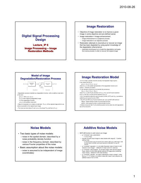
<strong>Digital</strong> <strong>Signal</strong> <strong>Processing</strong><br />
<strong>Design</strong><br />
g<br />
Lecture_IP 6<br />
<strong>Image</strong> <strong>Processing</strong> – <strong>Image</strong><br />
<strong>Restoration</strong> Methods<br />
Model of <strong>Image</strong><br />
Degradation/<strong>Restoration</strong> Process<br />
i Degradation process modeled as a degradation function, with an additive noise term,<br />
of the form:<br />
gxy ( , ) = Hfxy [ ( , )] + η(<br />
xy , )<br />
f( x, y)<br />
is the original (undegraded) image<br />
H is the degradation function<br />
η(<br />
xy , ) is the additive noise term<br />
i Object of restoration is to obtain an estimate, fˆ( x, y),<br />
of the original image which is as<br />
close as possible to the original input image.<br />
i The more we know about<br />
H and η(<br />
x, y), the closer fˆ( x, y)will be to f( x, y)<br />
Noise Models<br />
• Two basic types of noise models:<br />
– noise in the spatial domain; described by a<br />
noise probability density function<br />
– noise in the frequency domain; described by<br />
various Fourier properties of the noise<br />
• Basic assumption about the noise models:<br />
– noise is assumed to be independent of image<br />
(coordinates)<br />
<strong>Image</strong> <strong>Restoration</strong><br />
• Objective of image restoration is to improve a given<br />
image in some objective and pre-defined sense<br />
• <strong>Image</strong> restoration ≠ <strong>Image</strong> enhancement<br />
– image enhancement is a subjective process<br />
– image restoration is an objective process<br />
• <strong>Restoration</strong> attempts to reconstruct or recover an image<br />
that has been degraded by using apriori knowledge of<br />
the degradation phenomenon<br />
– restoration techniques try to model the degradation and apply<br />
the inverse process in order to recover the original image<br />
<strong>Image</strong> <strong>Restoration</strong> Model<br />
i If H is a linear, spatially invariant process, the degraded image is given<br />
in the spatial domain by:<br />
gxy ( , ) = hxy ( , ) ∗ fxy ( , ) + η(<br />
xy , )<br />
where hxy ( , ) is the spatial representation of the degradation function<br />
and<br />
symbol ∗ denotes convolution.<br />
i In the frequency domain we can describe the process as:<br />
G ( uv , ) = Huv ( , ) ⋅ F ( uv , ) + Nuv ( , )<br />
where Fuv ( , ) is the Fourier transform of f( xy , ), Huv ( , )is the Fourier transform<br />
of hxy ( , ) and Nuv ( , )is the Fourier transform of η(<br />
xy , )<br />
i H( u, v) sometimes called the optical transfer function (OTF) and h( x, y)<br />
sometimes<br />
called the point spread function (PSF)<br />
i The OTF and PSF are a Fourier transform pair; can use MATLAB functions:<br />
otf2psf - optical transfer function to point spread function<br />
psf2otf - point spread function to optical transfer function<br />
i Initially we assume<br />
that H is the identity operator and we deal only with degradation<br />
due to the noise term<br />
Additive Noise Models<br />
• MATLAB function to add noise to an image:<br />
– g = imnoise(f, type, parameters)<br />
• f is input image<br />
– imnoise converts input image to class double with range [0, 1] before<br />
adding noise<br />
• to add Gaussian G noise of mean 64 6 and variance 400 00 to an uint8 8 image, g , need<br />
to scale mean to 64/255, and scale variance to 400/(255) 2 for input to<br />
imnoise<br />
– g = imnoise(f, ‘gaussian’, m, var) adds Gaussian noise of mean m and<br />
variance var to image f. (Default is 0 mean and 0.01 variance)<br />
– g = imnoise(f, ‘salt & pepper’, d) corrupts image f with salt and pepper<br />
noise, where d is the noise density (percent of image area containing<br />
noise values). (Default is 0.05 noise density).<br />
– g = imnoise(f, ‘speckle’, var) adds multiplicative noise to image f, using<br />
form g = f + n*f, where n is uniform noise with mean 0 and variance var.<br />
(Default value of var is 0.04).<br />
2010-08-26<br />
1
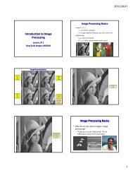
f=imread(‘lena.tif’);<br />
Lena Original <strong>Image</strong><br />
g=imnoise(f,’gaussian’,0,0.01);<br />
mean=0, variance=0.01;<br />
g=imnoise(f,’gaussian’,0,0.001);<br />
mean=0, variance=0.001;<br />
g=imnoise(f,’gaussian’,0,0.1);<br />
mean=0, variance=0.1;<br />
Upper Left: lena original; Upper Right: lena with salt & pepper noise at 0.01; Lower Left:<br />
lena with salt & pepper noise at 0.1; Lower Right: lena with salt & pepper noise at 1.0<br />
Noise Models<br />
Lena original; Lena with poisson noise added<br />
Additive Noise Models<br />
• g = imnoise(f, type, parameters)<br />
– g = imnoise(f, ‘gaussian’, m, var); % Gaussian noise<br />
of mean m and variance var; default is m = 0, var =<br />
0.01<br />
– g = imnoise(f imnoise(f, ‘salt salt & pepper’ pepper , d); adds salt and<br />
pepper noise, where d is the noise density (i.e.,<br />
percent of image area containing noise values)<br />
– g = imnoise(f, ‘speckle’, var); adds multiplicative noise<br />
using equation g = f + n.*f, where n is uniformly<br />
distributed random noise with mean 0 and variance<br />
var; default var = 0.004<br />
– g = imnoise(f, ‘poisson’); generates Poisson noise<br />
from data<br />
Upper Left: lena original; Upper Right: lena with speckle noise at 0.004; Lower<br />
Left: lena with speckle noise at 0.04; Lower Right: lena with speckle noise at 0.4<br />
Summary<br />
of Noise<br />
Models<br />
2010-08-26<br />
2
Original <strong>Image</strong> (lena.tif)<br />
Noise Models<br />
<strong>Image</strong> corrupted by Gaussian<br />
noise of mean 0, variance<br />
400/(255*255)<br />
Noise with Specified Distribution<br />
• Sometimes want to generate noise with a given<br />
probability density function (PDF) or a given<br />
cummulative distribution function (CDF)<br />
i If f w is a uniformly f distributed random variable in the interval (0 (0, 1) 1),<br />
then we can obtain a random variable z with a specified CDF, Fz,<br />
by<br />
solving the equation<br />
−1<br />
z = Fz( w)<br />
or, equivalently, by finding<br />
a solution to the equation<br />
Fz( z) = w<br />
Noise Distributions in the<br />
Real World<br />
• Gaussian noise occurs in imaging sensors<br />
operating at low light levels<br />
• Salt-and-pepper p pp noise arises in faulty y<br />
switching devices<br />
• Rayleigh noise arises in range imaging<br />
• Exponential and Erlang noise occur in<br />
laser imaging<br />
<strong>Image</strong> corrupted by ‘salt &<br />
pepper’ noise with density 0.1<br />
Noise Models<br />
<strong>Image</strong> corrupted by ‘speckle’<br />
noise with mean 0 and variance<br />
0.04<br />
Noise with Specified Distribution<br />
i Assume a uniform random number, w,<br />
in the interval (0, 1), and<br />
we wish to generate random numbers, z,<br />
with a Rayleigh CDF of the form:<br />
2<br />
⎧ −( z−a) / bfor<br />
z ≥ a⎫<br />
⎪1−<br />
e<br />
Fz( z)<br />
= ⎨ ⎬<br />
⎪⎩ 0 for z < a⎭<br />
where b > 0. To find z we solve the equation<br />
2<br />
−( z−a) / b<br />
1−<br />
e = w<br />
z = a + − b ln(1 − w )<br />
i MATLAB: R = a + sqrt(-b*log(1-rand(M, N)));<br />
Rayleigh CDF with a=0,<br />
b=1<br />
Generation of RVs<br />
2010-08-26<br />
3
MATLAB Noise Generation<br />
• A = rand(M, N) – generates M x N array of uniformly<br />
distributed numbers in interval (0, 1)<br />
• A = randn(M, N) – generates M x N array of Gaussian<br />
distributed numbers with zero mean and unit variance<br />
• g = imnoise(f, type, parameters) – adds M x N array of<br />
noise of various types (e.g., ‘gaussian’, ‘salt & pepper’,<br />
‘speckle’, ‘poisson’) to an existing image, f<br />
• R = imnoise2(type, M, N, a, b) – generates M x N array<br />
of noise of types (‘uniform’,’gaussian’,’salt &<br />
pepper’,’lognormal’,’rayleigh’,’exponential’,’erlang’)<br />
– no scaling of noise array to (0, 1) interval<br />
– ‘salt & pepper’ noise has three values – 0 for pepper noise, 1 for<br />
salt noise, and 0,5 for no noise<br />
Random Number Histograms<br />
R = imnoise2(‘gaussian’, 10000, 1 0 1);<br />
P = hist(r, bins); -- bins=50<br />
Estimating Noise Parameters<br />
i Let z be a discrete random variable that denotes intensity levels in an image,<br />
i<br />
and let pz ( i ), i= 0,1,2,..., L−1,<br />
be the corresponding normalized histogram,<br />
where L is the number of possible intensity values.<br />
A histogram component,<br />
pz ( i ), is an estimate of the probability of occurrence of intensity value zi,<br />
and<br />
the histogram may be viewed as an approximation of the intensity PDF.<br />
i Use the histogram central moment to describe histogram shape, i.e.,<br />
L L−<br />
1<br />
n<br />
n = ∑ zi −m<br />
p zi<br />
i = 0<br />
μ ( ) ( )<br />
where n is the moment order, and m is the mean:<br />
L−1<br />
m = ∑ zip( zi)<br />
i = 0<br />
i Since the histogram is normalized (to a sum of 1.0), we<br />
see that μ0 = 1, μ1<br />
= 0, and<br />
the second moment is the variance, i.e.,<br />
L−1<br />
2<br />
μ = ( z −m)<br />
p( z )<br />
2<br />
∑<br />
i i<br />
i = 0<br />
Salt & Pepper Noise<br />
• Salt & Pepper noise viewed as generating an image with three<br />
values; e.g., for uint8 images (with eight bits)<br />
– value 1 – 0, with probability Pp, – value 2 – 255, with probability Ps, – value 3 –k,with probability (1-(Pp+ Ps)) where k is any number between<br />
the two extremes<br />
• Denote the generated noise as r(x,y); the salt & pepper corrupted<br />
image is obtained by assigning a 0 to all locations in f where a 0<br />
occurs in r; similarly assigning a 255 to all locations in f where 255<br />
occurs in r; finally we leave unchanged in f all locations in which r<br />
contains the value k<br />
• P= Pp+ Ps called the noise density; if Pp=0.02 and Ps=0.01, then<br />
approximately 2% of pixels are corrupted by pepper noise, 1% are<br />
corruped by salt noise, and the noise density is 0.03.<br />
Estimating Noise Parameters<br />
• Need to estimate noise parameters from<br />
the image data<br />
– generally estimate mean, m, and variance, σ2 ,<br />
and then convert to noise distribution<br />
parameters a and b to specify PDF of interest<br />
Estimating Noise Parameters<br />
• MATLAB code for estimating moments of a<br />
distribution:<br />
– [v, unv] = statmoments(p, n);<br />
– v(1) = m (mean);<br />
– v(k) = μ k, k=2,3,…,n<br />
– v contains normalized moments based on random<br />
variable scaled to range [0, 1]<br />
– unv contains same moments as v but computed with<br />
the data in its original range of values<br />
– p is histogram vector (size(p)=256 for uint8 images)<br />
– n number of moments to compute<br />
2010-08-26<br />
4
Estimating Noise Parameters<br />
• Often noise parameters estimated directly from a<br />
given noisy image<br />
• Approach is to select a region of the image with<br />
as featureless a background g as p possible ( (ROI –<br />
Region of Interest)<br />
– B = roipoly(f, c, r); % polygonal ROI<br />
– f = image<br />
– c and r are vectors of column and row coordinates of<br />
the vertices of the polygon<br />
– B is binary image, same size as f, with 0’s outside<br />
ROI and 1’s inside<br />
Regions of Interest<br />
(a) Noisy image<br />
(b) Mask, B, generated<br />
interactively using command:<br />
[B, c, r] = roipoly(f);<br />
(c) Histogram of ROI generated<br />
using command:<br />
[h, npix] = histroi(f, c,r);<br />
figure, bar(h, 1);<br />
(d) Mean and variance of region<br />
masked by B obtained using<br />
command:<br />
[v, unv] = statmoments(h, 2);<br />
v=[0.5803, 0.0063] ;<br />
unv=[147.9814, 407.8679];<br />
Histogram of Gaussian noise<br />
with same mean and variance<br />
as estimated above.<br />
Spatial Noise Filters<br />
Estimating Noise Parameters<br />
• Interactively<br />
finding the ROI:<br />
– B = roipoly(f); %<br />
user specifies a<br />
polygon using the<br />
mouse and the set<br />
of commands at<br />
right side of figure<br />
<strong>Restoration</strong> – Noise Only Case<br />
i When the only degradation is noise, the model is:<br />
gxy ( , ) = f( xy , ) + η(<br />
xy , )<br />
i Method of choice for restoration is spatial filtering.<br />
i SSpatial ti l filt filters of f iinterest: t t<br />
− Sxy denotes an mxn subimage (region) of noisy input image g<br />
− ( xy , ) is set of coordinates at center of region<br />
− fˆ( x, y) is an estimate of f( x, y),<br />
the filter response at ( xy , )<br />
i The linear filters of the table (on next slide) are implemented using imfilter<br />
i The median non-linear filteris implemented using medfilt2<br />
i The max and min filters are implemented using imdilate and imerode<br />
i MATLAB routine spfile implements all these filters in the spatial domain<br />
<strong>Restoration</strong> Example – Noise<br />
Only Case<br />
Figure in (a) – pepper noise only<br />
[M, N] = size(f);<br />
R = imnoise2(salt & pepper’, M, N, 0.1, 0);<br />
gp = f;<br />
gp(R == 0) = 0;<br />
Figure in (b) – salt noise only<br />
R = imnoise2(‘salt imnoise2( salt % pepper’ pepper , MM, NN, 00, 00.1); 1);<br />
gs = f;<br />
gs(R == 1) = 255;<br />
Figure in (c) – contraharmonic filtering of (a)<br />
fp = spfilt(gp, ‘chmean’, e, e, 1.5);<br />
Figure in (d) – contraharmonic filtering of (b)<br />
fs = spfilt(gs, ‘chmean’, 3, 3, -1.5);<br />
Figures in (e) and (f) – max (part (a)) and<br />
min (part (b)) filters<br />
fpmax = spfilt(gp, ‘max’, 3, 3);<br />
fsmin = spfilt(gs, ‘min’, 3, 3);<br />
2010-08-26<br />
5
MATLAB Find Function<br />
• I = find(A) – I contains all the indices of array A that point to nonzero<br />
elements<br />
• [r, c] = find(A) – returns the row and column indices of non-zero<br />
elements of A<br />
• [r, c, v] = find(A) – returns also the nonzero values in A in column<br />
vector v<br />
• Example: find and set to 0 all pixels in A whose values are less than<br />
8<br />
– I = find(A < 8);<br />
A(find(A= 64 & A = 64 & A motion of 9 pixels in the horizontal direction<br />
2010-08-26<br />
6
Degraded <strong>Image</strong> Creation<br />
• use MATLAB function imfilter to create degraded image<br />
with a PSF that is either known or computed (as in<br />
previous slide):<br />
g = imfilter(f, PSF, ‘circular’); % minimize border effects<br />
• add appropriate noise to model degraded image<br />
g = g + noise; % noise same size as g; generated using one of<br />
methods discussed previously<br />
• use checkerboard pattern as image example<br />
c = checkerboard(NP, M, N); % NP= number pixels on the side<br />
of each square; M row; N columns;<br />
% light squares on left half are white; light squares on right half<br />
are gray; all light squares white using<br />
K = checkerboard(NP, M, N) > 0.5; % range of K is [0 1] (class<br />
double)<br />
Degraded <strong>Image</strong> <strong>Restoration</strong><br />
• Method 1 – Direct Inverse Filtering<br />
– ignore noise term<br />
– form estimate of the form:<br />
ˆ Guv ( , )<br />
Fuv ( , )<br />
=<br />
Huv ( , )<br />
– where G(u,v) is the FT of the degraded<br />
image, and H(u,v) is the FT of the estimated<br />
blurring filter<br />
– take the inverse Fourier transform as the<br />
estimate of the deblurred image<br />
Degraded <strong>Image</strong> <strong>Restoration</strong><br />
i Weiner filtering solution; seek an estimate, fˆ,<br />
that minimizes<br />
the statistical error function:<br />
2 2<br />
e = E{ ( f −fˆ)<br />
}<br />
where E is the expected value operator, and f is the undegraded<br />
image.<br />
i Th The solution l ti (i (in<br />
th the frequency f domain) d i ) is: i<br />
⎡ 2<br />
ˆ<br />
1 | Huv ( , )| ⎤<br />
Fuv ( , ) = ⎢ ( , )<br />
2<br />
⎥ Guv<br />
⎢⎣Huv ( , ) | Huv ( , )| + Sη( uv , )/ Sf( uv , ) ⎥⎦<br />
where:<br />
Huv ( , ) is the degradation function<br />
2<br />
Sη( u, v) = | N( u, v)<br />
| is the power spectrum of the noise<br />
2<br />
Sf<br />
( uv , ) = | Fuv ( , ) | is the power spectrum of the undegraded image<br />
S ( u, v) / S ( u, v ) is called the noise - to - signal power ratio<br />
η<br />
f<br />
Degraded <strong>Image</strong> Creation<br />
(a) f = checkerboard(8); % 8 x<br />
8 image of class double<br />
(b) PSF = fspecial(‘motion’, 7,<br />
45); % spatial filter<br />
gb = imfilter(f, PSF,<br />
‘circular’);<br />
(c) Gaussian noise image with<br />
mean 0 and variance 0.001<br />
noise =<br />
imnoise2(‘Gaussian’,<br />
size(f,1), size(f,2), 0,<br />
sqrt(0.001));<br />
(d) g = gb + noise;<br />
Degraded <strong>Image</strong> <strong>Restoration</strong><br />
• Method 2 – Direct Inverse Filter with Noise Term<br />
– include noise term<br />
– form estimate of the form:<br />
ˆ Nuv ( , )<br />
Fuv ( , ) = Fuv ( , ) +<br />
Huv ( , )<br />
– shows that even if we knew H(u,v) exactly we could<br />
not recover F(u,v) exactly because the noise<br />
component is a random function whose FT, N(u,v), is<br />
not known.<br />
– typical approach is to use Method 1 in limited<br />
frequency range<br />
Degraded <strong>Image</strong> <strong>Restoration</strong><br />
i Wiener filtering solution (simplified)<br />
i Compute average noise and image power, i.e.,<br />
1<br />
η A = ∑∑Sη(<br />
u, v)<br />
MN u v<br />
1<br />
f fA = ∑∑ S Sf ( u u, v )<br />
MN u v<br />
i Compute ratio:<br />
ηA<br />
R =<br />
fA<br />
i Utilize constant R in place of function Sη( u, v)<br />
/ Sf( u, v)<br />
for simple approximation to ideal Wiener filter (called<br />
parametric Wiener filter)<br />
2010-08-26<br />
7
MATLAB Implementation of<br />
Wiener Filter<br />
• MATLAB Code: g is degraded image, frest is the<br />
restored image, 3 possible implementations<br />
frest = deconvwnr(g, PSF);<br />
• assumes noise-to-signal ratio is zero; result same as<br />
inverse filter<br />
frest = deconvwnr(g, PSF, NSPR);<br />
• assumes noise-to-signal ratio is known, either as a<br />
constant or as an array<br />
frest = deconvwnr(f, PSF, NACORR, FACORR);<br />
• assumes that the autocorrelation functions, NACORR<br />
and FACORR of the noise and the undegraded image<br />
are known<br />
Beyond Wiener Filtering<br />
• Previous example assumed that the original image and<br />
noise functions were known<br />
– hence we were able to estimate the correct parameters<br />
– result in part (d) is that best that can be accomplished with<br />
Wiener deconvolution in this case<br />
– challenge, in practice, is to choose appropriate functions for the<br />
blur and noise when these quantities are not known apriori.<br />
• Other solutions:<br />
– constrained least squares filtering<br />
– iterative nonlinear restoration using the Lucy-<br />
Richardson algorithm<br />
– blind deconvolution<br />
– image reconstruction from projections<br />
Wiener Filtering<br />
Summary<br />
(b) frest1 = deconvwnr(g, PSF); % noise<br />
dominates image<br />
(c) computed ratio R as:<br />
Sn = abs(fft2(noise)).^2; noise power spectrum<br />
nA = sum(Sn(:))/numel(noise); % noise<br />
average power<br />
Sf = abs(fft2(f)).^2; % image power spectrum<br />
fA = sum(Sf(:))/numel(f); % image average<br />
power<br />
R = nAfA;<br />
frest2 = deconvwnr(g, PSF, R);<br />
(d) use autocorrelations:<br />
NCORR = fftshift(real(ifft2(Sn)));<br />
ICORR = fftshift(real(ifft2(Sf)));<br />
frest3 = deconvwnr(g, PSF, NCORR, ICORR);<br />
• Methods of <strong>Image</strong> <strong>Restoration</strong><br />
– model degradation (assuming apriori knowledge of degradation filter, H, and noise statistics, η)<br />
– apply inverse process to degradation<br />
• Noise Models<br />
– spatial/frequency domain models<br />
– use MATLAB routine imnoise to add noise to image; Gaussian, salt & pepper, speckle,<br />
Poisson, etc.<br />
• Generate Noise with Specified PDF or CDF<br />
– use MATLAB routine imnoise2<br />
• Estimate Noise Statistics<br />
– use MATLAB routine statmoments<br />
– use regions of interest for better estimates<br />
• Noise Only <strong>Restoration</strong><br />
– use linear, median, min, max spatial filters<br />
– use adaptive spatial filters for better estimates<br />
• <strong>Image</strong> Blur With Noise<br />
– direct inverse filtering methods<br />
– Wiener filtering method<br />
– alternative approaches<br />
2010-08-26<br />
8