Time Domain Methods in Speech Processing
Time Domain Methods in Speech Processing
Time Domain Methods in Speech Processing

Create successful ePaper yourself
Turn your PDF publications into a flip-book with our unique Google optimized e-Paper software.
Digital Signal Process<strong>in</strong>g<br />
Design — Lecture 5<br />
<strong>Time</strong> <strong>Doma<strong>in</strong></strong> <strong>Methods</strong><br />
<strong>in</strong> <strong>Speech</strong> Process<strong>in</strong>g<br />
1
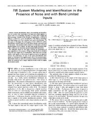
General Synthesis Synthesis Model<br />
T T<br />
T 1<br />
T 2<br />
voiced sound<br />
amplitude<br />
unvoiced sound<br />
amplitude<br />
Log Areas, Reflection<br />
Coefficients, Formants, Vocal<br />
T Tract Polynomial, P l i l Articulatory<br />
A i l<br />
Parameters, …<br />
Rz ( ) = 1−<br />
z<br />
1<br />
α −<br />
Pitch Detection, Voiced/Unvoiced/Silence Detection, Ga<strong>in</strong> Estimation, Vocal Tract<br />
Parameter Estimation, Glottal Pulse Shape, Radiation Model<br />
2
Fundamental Fundamental Assumptions<br />
Assumptions<br />
• properties of the speech signal change relatively<br />
slowly l l with ith ti time (5 (5-10 10 sounds d per second) d)<br />
– over very short (5-20 msec) <strong>in</strong>tervals => uncerta<strong>in</strong>ty<br />
due to small amount of data, , vary<strong>in</strong>g y g p pitch, , vary<strong>in</strong>g y g<br />
amplitude<br />
– over medium length (20-100 msec) <strong>in</strong>tervals =><br />
uncerta<strong>in</strong>ty due to changes <strong>in</strong> sound quality quality,<br />
transitions between sounds, rapid transients <strong>in</strong><br />
speech<br />
– over long (100 (100-500 500 msec) <strong>in</strong>tervals => uncerta<strong>in</strong>ty<br />
due to large amount of sound changes<br />
• there is always y uncerta<strong>in</strong>tyy <strong>in</strong> short time<br />
measurements and estimates from speech<br />
signals<br />
3
Compromise Compromise Solution<br />
• “short-time” process<strong>in</strong>g p g methods => short segments g of<br />
the speech signal are “isolated” and “processed” as if<br />
they were short segments from a “susta<strong>in</strong>ed” sound with<br />
fixed (non-time-vary<strong>in</strong>g) ( y g) pproperties p<br />
– this short-time process<strong>in</strong>g is periodically repeated for the<br />
duration of the waveform<br />
– these short analysis segments, or “analysis frames” often<br />
overlap one another<br />
– the results of short-time process<strong>in</strong>g can be a s<strong>in</strong>gle number (e.g.,<br />
an estimate of the pitch period with<strong>in</strong> the frame), or a set of<br />
numbers (an estimate of the formant frequencies for the analysis<br />
frame)<br />
– the end result of the process<strong>in</strong>g is a new, time-vary<strong>in</strong>g sequence<br />
that serves as a new representation of the speech signal<br />
4
Frame Frame-by by-Frame Frame Process<strong>in</strong>g<br />
<strong>in</strong> Successive W<strong>in</strong>dows<br />
Frame 1<br />
Frame 2<br />
Frame 3<br />
Frame 4<br />
Frame 5<br />
75% frame overlap => frame length=L, frame shift=R=L/4<br />
Frame1={x[0],x[1],…,x[L-1]}<br />
Frame2={x[R] Frame2={x[R],x[R+1],…,x[R+L-1]}<br />
x[R+1] x[R+L-1]}<br />
Frame3={x[2R],x[2R+1],…,x[2R+L-1]}<br />
…<br />
5
Frame 1: samples 0,1,..., L −1<br />
Frame 2: samples RR , + 1,..., 1 R + L L−1<br />
1<br />
Frame 3: samples 2 R, 2R+ 1,..., 2R+ L−1<br />
Frame 4: samples 3 R,3R+ 1,...,3R+ L−1
Frame Frame-by by-Frame Frame Process<strong>in</strong>g <strong>in</strong> Successive W<strong>in</strong>dows<br />
• <strong>Speech</strong> is processed frame-by-frame <strong>in</strong> overlapp<strong>in</strong>g <strong>in</strong>tervals until entire<br />
region of speech is covered by at least one such frame<br />
• Results of analysis of <strong>in</strong>dividual frames used to derive model parameters <strong>in</strong><br />
some manner<br />
• Representation goes from time sample x[<br />
n],<br />
n = , 0,<br />
1,<br />
2,<br />
to parameter<br />
vector f[ nˆ], n= ˆ 0,1,2, where n is the time <strong>in</strong>dex and ˆn<br />
is the frame <strong>in</strong>dex.<br />
7
Short Short-<strong>Time</strong> Short <strong>Time</strong> Signal Process<strong>in</strong>g<br />
Short Short-<strong>Time</strong> <strong>Time</strong> Parameter<br />
sn [ ] Analysis Q Estimation f [ nˆ<br />
]<br />
speech<br />
waveform<br />
Model Parameter(s):<br />
• speech/non-speech<br />
• voiced/unvoiced/background<br />
• pitch period (when voiced)<br />
• formants<br />
ˆn<br />
alternate<br />
model<br />
representation<br />
p parameter(s)<br />
p ( )<br />
8
Generic Short Short-<strong>Time</strong> Short <strong>Time</strong> <strong>Time</strong> Process<strong>in</strong>g<br />
Process<strong>in</strong>g<br />
∞ ⎛ ⎞<br />
Q ∑<br />
nˆ<br />
= ⎜ ∑ T ( x[ m]) ) w[ n−m] ⎟<br />
⎝ ⎠<br />
m=−∞ n= nˆ<br />
x[n] T(x[n])<br />
T( ) w[n]<br />
Qˆn<br />
l<strong>in</strong>ear or non-l<strong>in</strong>ear<br />
transformation<br />
w<strong>in</strong>dow sequence<br />
(usually ( y f<strong>in</strong>ite length) g )<br />
Qˆn<br />
• is a sequence of local weighted g average g<br />
values of the sequence T(x[n]) at time ˆ<br />
n= n<br />
9
Short Short-<strong>Time</strong> Short <strong>Time</strong> Energy<br />
∞<br />
∑<br />
m=−∞<br />
2<br />
[ ]<br />
E = ∑ x m<br />
-- this is the long term def<strong>in</strong>ition of signal energy<br />
-- there is little or no utility of this def<strong>in</strong>ition for time-vary<strong>in</strong>g signals<br />
Enˆ= ∑<br />
2<br />
x m<br />
ˆ n<br />
m= nˆ− L+<br />
1<br />
[ ]<br />
-- short-time energy <strong>in</strong> vic<strong>in</strong>ity of time nˆ<br />
2<br />
T ( x ) = x<br />
wn [ ] = 1 0≤n≤L−1 = 0 otherwise<br />
2 2<br />
= x [ nˆ − L+ 1]<br />
+ ... + x [ nˆ]<br />
10
Computation of Short Short-<strong>Time</strong> <strong>Time</strong> Energy<br />
• w<strong>in</strong>dow jumps/slides across sequence of squared values, select<strong>in</strong>g <strong>in</strong>terval<br />
ffor process<strong>in</strong>g i<br />
E<br />
• what happens to ˆn as sequence jumps by 2,4,8,...,L samples ( ˆn is a lowpass<br />
function—so it can be decimated without lost of <strong>in</strong>formation; why is lowpass?)<br />
• effects of decimation depend on L; if L is small, then ˆn is a lot more variable<br />
than if L is large (w<strong>in</strong>dow bandwidth changes with L!)<br />
E<br />
E<br />
E<br />
ˆn<br />
11
Effects Effects of of W<strong>in</strong>dow<br />
W<strong>in</strong>dow<br />
Q = T( x[ n]) ∗w[<br />
n]<br />
nˆ n= nˆ<br />
= x′ n ∗w n ˆ<br />
[ ] [ ]<br />
n= n<br />
• w[n] serves as a lowpass filter on T(x[n]) which often has a lot of<br />
high frequencies (most non-l<strong>in</strong>earities <strong>in</strong>troduce significant high<br />
frequency energy—th<strong>in</strong>k of what (x[n] x[n]) does <strong>in</strong> frequency)<br />
•often ft we extend t d the th def<strong>in</strong>ition d fi iti of f Q Qˆn<br />
tto <strong>in</strong>clude i l d a pre-filter<strong>in</strong>g filt i tterm<br />
so that x[n] itself is filtered to a region of <strong>in</strong>terest<br />
xˆ[ n] x[n]<br />
T(x[n])<br />
ˆn<br />
T( )<br />
L<strong>in</strong>ear<br />
Filter<br />
Lowpass<br />
Filter, w[n]<br />
Q<br />
12
Short Short-<strong>Time</strong> Short <strong>Time</strong> Energy<br />
• serves to differentiate voiced and unvoiced sounds <strong>in</strong> speech<br />
from silence (background signal)<br />
• natural def<strong>in</strong>ition of energy of weighted signal is:<br />
∞<br />
∑<br />
2<br />
E ˆ<br />
nˆ<br />
= ⎡⎣x[ m] w[ n−m] ⎤⎦<br />
(sum of squares of portion of signal)<br />
m=−∞<br />
-- concentrates measurement at sample n nˆ, us<strong>in</strong>g weight<strong>in</strong>g w [ n- nˆ m<br />
]<br />
nˆ<br />
∞<br />
= ∑<br />
2 2 ˆ −<br />
∞<br />
= ∑<br />
2 ˆ −<br />
m=−∞<br />
2<br />
m=−∞<br />
E x [ m] w [ n m] x [ m] h[ n m]<br />
h [ n ] = w [ n ]<br />
x[n] x2 x[n] x [n] E ˆ − short-time energy gy<br />
( ) 2 h[n]<br />
n<br />
13
Short Short-<strong>Time</strong> Short <strong>Time</strong> <strong>Time</strong> Energy Properties<br />
• depends on choice of h[n], or equivalently,<br />
w<strong>in</strong>dow i d w[n] [ ]<br />
–if w[n] duration very long and constant amplitude<br />
(w[n]=1, ( [ ] , n=0,1,...,L-1), , , , ), Enˆn<br />
would not change g much over<br />
time, and would not reflect the short-time amplitudes of<br />
the sounds of the speech<br />
– very long duration w<strong>in</strong>dows correspond to narrowband<br />
lowpass filters<br />
– want E ˆn to change at a rate comparable to the chang<strong>in</strong>g<br />
sounds of the speech => this is the essential conflict <strong>in</strong><br />
all speech process<strong>in</strong>g, namely we need short duration<br />
w<strong>in</strong>dow to be responsive to rapid sound changes, but<br />
short w<strong>in</strong>dows will not provide sufficient averag<strong>in</strong>g to<br />
give smooth and reliable energy function<br />
14
W<strong>in</strong>dows<br />
• consider two w<strong>in</strong>dows, w[n]<br />
– rectangular w<strong>in</strong>dow:<br />
• h[n]=1, 0≤n≤L-1 and 0 otherwise<br />
– Hamm<strong>in</strong>g w<strong>in</strong>dow (raised cos<strong>in</strong>e w<strong>in</strong>dow):<br />
• h[n]=0.54-0.46 cos(2πn/(L-1)), 0≤n≤L-1 and 0 otherwise<br />
– rectangular w<strong>in</strong>dow gives equal weight to all L<br />
samples <strong>in</strong> the w<strong>in</strong>dow (n,...,n-L+1)<br />
– Hamm<strong>in</strong>g g w<strong>in</strong>dow ggives most weight g to middle<br />
samples and tapers off strongly at the beg<strong>in</strong>n<strong>in</strong>g and<br />
the end of the w<strong>in</strong>dow<br />
15
Rectangular and Hamm<strong>in</strong>g W<strong>in</strong>dows<br />
<strong>Time</strong> Responses of L=21 L 21 po<strong>in</strong>t Rectangular and<br />
Hamm<strong>in</strong>g w<strong>in</strong>dows; Frequency Responses of L=51<br />
po<strong>in</strong>t Rectangular and Hamm<strong>in</strong>g W<strong>in</strong>dows<br />
16
W<strong>in</strong>dow W<strong>in</strong>dow Frequency Frequency Responses<br />
Responses<br />
• rectangular g w<strong>in</strong>dow<br />
s<strong>in</strong>( ΩLT<br />
/ 2)<br />
He ( ) =<br />
e<br />
s<strong>in</strong>( Ω T / 2 )<br />
jΩT −jΩT( L−1)/<br />
2<br />
• first zero occurs at f=Fs/L=1/(LT) (or Ω=(2π)/(LT)) =><br />
nom<strong>in</strong>al cutoff frequency of the equivalent “lowpass” lowpass filter<br />
• Hamm<strong>in</strong>g w<strong>in</strong>dow<br />
w [ n ] = 0.54 w [ n ] −0.46*cos(2 ( π n/( ( L−1)) )) w [ n ]<br />
H R R<br />
• can decompose Hamm<strong>in</strong>g W<strong>in</strong>dow FR <strong>in</strong>to comb<strong>in</strong>ation<br />
of three terms<br />
17
W<strong>in</strong>dow Frequency Responses<br />
Rectangular W<strong>in</strong>dows,<br />
L=21,41,61,81,101<br />
Hamm<strong>in</strong>g W<strong>in</strong>dows,<br />
L=21,41,61,81,101<br />
18
RW and HW Frequency Responses<br />
•bandwidth of HW is approximately twice the bandwidth of RW<br />
• attenuation of more than 40 dB for HW outside passband,<br />
versus 14 dB ffor RW<br />
• stopband attenuation is essentially <strong>in</strong>dependent of L, the<br />
w<strong>in</strong>dow duration => <strong>in</strong>creas<strong>in</strong>g L simply decreases w<strong>in</strong>dow<br />
bandwidth<br />
• L needs to be larger than a pitch period (or severe<br />
fluctuations will occur <strong>in</strong> E En), ) but smaller than a sound duration<br />
(or En will not adequately reflect the changes <strong>in</strong> the speech<br />
signal)<br />
There is no perfect value of L, s<strong>in</strong>ce a pitch period can be as short as 20 samples (500 Hz at a 10 kHz<br />
sampl<strong>in</strong>g rate) for a high pitch child or female, and up to 250 samples (40 Hz pitch at a 10 kHz sampl<strong>in</strong>g<br />
rate) for a low pitch male; a compromise value of L on the order of 100-200 samples for a 10 kHz sampl<strong>in</strong>g<br />
rate is often used <strong>in</strong> practice<br />
19
Short Short-<strong>Time</strong> <strong>Time</strong> Energy us<strong>in</strong>g RW/HW<br />
E ˆn<br />
ˆn E<br />
L=51 L=51<br />
L=101 L=101<br />
L=201 L=201<br />
L=401 L=401<br />
•as L <strong>in</strong>creases, the plots tend to converge (however you are smooth<strong>in</strong>g sound energies)<br />
• short-time energy provides the basis for dist<strong>in</strong>guish<strong>in</strong>g voiced from unvoiced speech<br />
regions, and for medium-to-high SNR record<strong>in</strong>gs, can even be used to f<strong>in</strong>d regions of<br />
silence/background signal<br />
20
Short Short-<strong>Time</strong> <strong>Time</strong> Energy gy for AGC<br />
C Can use an IIR filt filter t to d def<strong>in</strong>e fi short short-time h t ti time energy, e.g.,<br />
•<br />
•<br />
time-dependent energy def<strong>in</strong>ition<br />
∞ ∞<br />
2 2<br />
∑ ∑<br />
σ [ n] = x [ m] h[ n−m]/ h[ m]<br />
m=−∞ m=<br />
0<br />
consider impulse response of filter of form<br />
n−1 n−1<br />
= − = ≥<br />
hn [ ] α un [ 1] α n 1<br />
= 0 n < 1<br />
∞<br />
2<br />
∑<br />
m=−∞<br />
2 n−m−1 σ [ n] = ∑ ( 1−α) x [ m] α u[ n−m−1] 21
Recursive Short Short-<strong>Time</strong> Short <strong>Time</strong> <strong>Time</strong> Energy<br />
i un [ −m−1] implies the condition n−m−1≥ 0<br />
or m ≤ n−<br />
1 giv<strong>in</strong>g i i<br />
i<br />
i<br />
i<br />
2<br />
−1<br />
∑<br />
=−∞<br />
2 − −1<br />
2 2<br />
n<br />
m ∞<br />
n m<br />
σ [ n] = ( 1− α) x [ m] α = ( 1−α)( x [ n− 1] + αx<br />
[ n−<br />
2]<br />
+ ...)<br />
for the <strong>in</strong>dex n −1<br />
we have<br />
n−2<br />
2 2 n−m−2 2 2<br />
∑<br />
σ [ n− 1 ] = ( 1− α ) x [ m ] α = ( 1−α )( x [ n− 2 ] + αx<br />
[ n−<br />
3 ] + ...) )<br />
m=−∞<br />
thus giv<strong>in</strong>g the relationship<br />
2 2 2<br />
σσ [ n ] = αα ⋅ ⋅σσ [ n − 1 ] + x [ n − 1 ]( 1 − −αα<br />
)<br />
and def<strong>in</strong>es an Automatic Ga<strong>in</strong> Control (AGC) of the form<br />
Gn [ ] =<br />
G<br />
0<br />
σ [ n]<br />
22
Recursive Short Short-<strong>Time</strong> Short <strong>Time</strong> <strong>Time</strong> Energy<br />
2 n<br />
x [n]<br />
2 x [ ]<br />
σ [ ]<br />
( )<br />
1<br />
z +<br />
−<br />
( ) z +<br />
( 1−<br />
α)<br />
α<br />
2 2 2<br />
σ [ n] = α ⋅σ [ n− 1] + x [ n−1](<br />
1−α)<br />
1<br />
z −<br />
2 n<br />
23
Recursive Short Short-<strong>Time</strong> Short <strong>Time</strong> <strong>Time</strong> Energy<br />
24
Use of Short Short-<strong>Time</strong> <strong>Time</strong> Energy gy for AGC<br />
25
Use of Short Short-<strong>Time</strong> <strong>Time</strong> Energy for AGC<br />
α =<br />
α =<br />
0.9<br />
0.99<br />
26
Short Short-<strong>Time</strong> Short <strong>Time</strong> Magnitude<br />
• short-time short time energy is very sensitive to large<br />
signal levels due to x2 [n] terms<br />
– consider a new def<strong>in</strong>ition of ‘pseudo-energy’ based<br />
on average signal magnitude (rather than energy)<br />
∞<br />
M ˆ | [ ]| [ ˆ<br />
n = ∑ n xm wn−m] ∑<br />
m=−∞<br />
– weighted sum of magnitudes, rather than weighted<br />
sum of squares<br />
x[n] |x[n]| Mnˆ= M n n= nˆ<br />
| | w[n]<br />
• computation avoids multiplications of signal with itself (the squared term)<br />
27
Short Short-<strong>Time</strong> <strong>Time</strong> Magnitudes<br />
g<br />
• differences between E n and M n noticeable <strong>in</strong> unvoiced regions<br />
M ˆn<br />
ˆn M<br />
L=51 L=51<br />
L=101 L=101<br />
L=201 L=201<br />
L=401 L=401<br />
• dynamic range of M Mn ~ square root (dynamic range of E En) ) => level differences between voiced and<br />
unvoiced segments are smaller<br />
• E n and M n can be sampled at a rate of 100/sec for w<strong>in</strong>dow durations of 20 msec or so => efficient<br />
representation of signal energy/magnitude<br />
28
Short <strong>Time</strong> Energy and Magnitude Magnitude—<br />
Rectangular R RRectangular t l W<strong>in</strong>dow Wi d<br />
E ˆn<br />
L=51 L=51<br />
M<br />
L=101 L=101<br />
L=201 L=201<br />
L=401 L=401<br />
ˆn<br />
29
Short <strong>Time</strong> Energy and Magnitude Magnitude—Hamm<strong>in</strong>g Hamm<strong>in</strong>g<br />
Wi W<strong>in</strong>dow d<br />
E ˆn<br />
L=51<br />
L=101<br />
L=201<br />
L=401<br />
M<br />
ˆn<br />
L=51<br />
L=101<br />
L=201<br />
L=401<br />
30
Short Short-<strong>Time</strong> Short <strong>Time</strong> <strong>Time</strong> Average ZC Rate<br />
zero cross<strong>in</strong>gs<br />
zero cross<strong>in</strong>g => successive samples<br />
have different algebraic signs<br />
• zero cross<strong>in</strong>g rate is a simple measure of the ‘frequency content’ of a<br />
signal—especially true for narrowband signals (e.g., s<strong>in</strong>usoids)<br />
• s<strong>in</strong>usoid at frequency F0 with sampl<strong>in</strong>g rate FS has FS/F0 samples per<br />
cycle with two zero cross<strong>in</strong>gs per cycle, giv<strong>in</strong>g an average zero<br />
cross<strong>in</strong>g g rate of<br />
z 1=(2) cross<strong>in</strong>gs/cycle x (F 0 / F S ) cycles/sample<br />
z z1=2F =2F 0 /F / FS cross<strong>in</strong>gs/sample (i (i.e., e z z1 proportional to F F0 )<br />
z M=M (2F 0 /F S ) cross<strong>in</strong>gs/(M samples)<br />
31
S<strong>in</strong>usoid S<strong>in</strong>usoid Zero Zero Cross<strong>in</strong>g Cross<strong>in</strong>g Rates<br />
Rates<br />
Ass Assume me the sampl<strong>in</strong>g rate is F FS<br />
= 10 10, 000 HHz<br />
1. F0 = 100 Hz s<strong>in</strong>usoid has FS/ F0<br />
= 10, 000 / 100 = 100 samples/cycle;<br />
or z1 = 2 / 100 cross<strong>in</strong>gs/sample, or z100<br />
= 2 / 100 * 100 =<br />
2 cross<strong>in</strong>gs/10 msec <strong>in</strong>terval<br />
2. F 0 = 1000 Hz s<strong>in</strong>usoid<br />
has F S / F 0 = 10, 000 / 1000 = 10 samples/cycle; p y<br />
or z1 = 2 / 10 cross<strong>in</strong>gs/sample, or z100<br />
= 2 / 10 * 100 =<br />
20 cross<strong>in</strong>gs/10 msec <strong>in</strong>terval<br />
3. F0 = 5000 Hz s<strong>in</strong>usoid has FS/ F0<br />
= 10, 000 / 5000 = 2 samples/cycle;<br />
or z = 2/ 2 cross<strong>in</strong>gs/sample,<br />
or z100<br />
= 2 / 2 * 100 =<br />
1<br />
100 cross<strong>in</strong>gs/10 msec <strong>in</strong>terval<br />
32
Zero Cross<strong>in</strong>g g for S<strong>in</strong>usoids<br />
1<br />
0.5<br />
0<br />
-0.5<br />
offset:0.75, 100 Hz s<strong>in</strong>ewave, ZC:9, offset s<strong>in</strong>ewave, ZC:8<br />
-1<br />
0 50 100 150 200<br />
1.5<br />
1<br />
0.5<br />
0<br />
Off Offset=0.75 0<br />
0 50 100 150 200<br />
100 Hz s<strong>in</strong>ewave<br />
100 Hz s<strong>in</strong>ewave with dc offset<br />
ZC=9<br />
ZC=8<br />
ZC 8<br />
33
Zero Cross<strong>in</strong>gs g for Noise<br />
3<br />
2<br />
1<br />
0<br />
-1<br />
-2<br />
6<br />
4<br />
0<br />
offseet:0.75, random noise, ZC:252, offset noise, ZC:122<br />
0 50 100 150 200<br />
Off Offset=0.75 0<br />
random gaussian noise<br />
random gaussian noise with dc offset<br />
ZC=252<br />
2 ZC=122<br />
-2<br />
0 50 100 150 200 250<br />
34
ZC Rate Def<strong>in</strong>itions<br />
1<br />
Znˆ= 2Leff<br />
∞<br />
∑ | sgn( x[ m]) −sgn( x[ m−1]) | w[ nˆ−m] m=−∞<br />
sgn( ( x [ n ]) = 1 x [ n ] ≥ 0<br />
=− 1 xn [ ] < 0<br />
i simple w<strong>in</strong>dow, rectangular with<br />
wn [ ] = 1 0≤n≤L−1 = 0 otherwise<br />
L = L<br />
i eff ff<br />
same form for Z n as for E n or M n<br />
35
ZC Normalization<br />
i Th The fformal l ddef<strong>in</strong>ition fi iti of f z iis:<br />
i<br />
nˆ<br />
1<br />
Znˆ= z1= ∑ | sgn( x[ m]) −sgn( x[ m−1])<br />
|<br />
L<br />
2 m= nˆ− L+<br />
1<br />
n<br />
is <strong>in</strong>terpreted as the number of zero cross<strong>in</strong>gs per sample.<br />
For most practical applications, we need the rate of zero cross<strong>in</strong>gs<br />
per fixed <strong>in</strong>terval of M samples, samples which is<br />
z = z ⋅ M = rate of zero cross<strong>in</strong>gs per M sample <strong>in</strong>terval<br />
M<br />
1<br />
Thus, for an <strong>in</strong>terval of τ sec., correspond<strong>in</strong>g to M samples we get<br />
z = z ⋅ M; M = τ F = τ / T<br />
M 1<br />
S<br />
36
ZC Normalization<br />
i For a 1000 Hz s<strong>in</strong>ewave as <strong>in</strong>put, us<strong>in</strong>g a 40 msec w<strong>in</strong>dow length<br />
i<br />
( L), with various values of sampl<strong>in</strong>g rate ( FS),<br />
we get the follow<strong>in</strong>g:<br />
F L z M z<br />
S 1<br />
M<br />
8000 320 1/ 4 80 20<br />
10000 400 1 / 5 100 20<br />
16000 640 1 / 8 160 20<br />
Thus us we e see tthat at tthe e normalized o a ed (pe (per <strong>in</strong>terval) te a ) zero e o ccross<strong>in</strong>g oss g rate, ate,<br />
zM,<br />
is <strong>in</strong>dependent of the sampl<strong>in</strong>g rate and can be used as a measure<br />
of the dom<strong>in</strong>ant energy <strong>in</strong> a band.<br />
37
ZC Rate Distributions<br />
1 KHz 2KHz 3KHz 4KHz<br />
• for voiced speech, energy is ma<strong>in</strong>ly below 1.5 kHz<br />
• for unvoiced speech speech, energy is ma<strong>in</strong>ly above 1.5 1 5 kHz<br />
• mean ZC rate for unvoiced speech is 49 per 10 msec <strong>in</strong>terval<br />
• mean ZC rate for voiced speech is 14 per 10 msec <strong>in</strong>terval<br />
Unvoiced <strong>Speech</strong> <strong>Speech</strong>: :<br />
the dom<strong>in</strong>ant energy energy gy<br />
component is at<br />
about 2.5 kHz<br />
Voiced <strong>Speech</strong> <strong>Speech</strong>: <strong>Speech</strong> <strong>Speech</strong>: :the : the<br />
dom<strong>in</strong>ant energy<br />
component is at<br />
about 700 Hz<br />
38
ZC Rates for <strong>Speech</strong><br />
• 15 msec<br />
w<strong>in</strong>dows<br />
• 100/sec<br />
sampl<strong>in</strong>g rate on<br />
ZC computation<br />
39
Short Short-<strong>Time</strong> <strong>Time</strong> Energy, Magnitude, ZC<br />
40
Issues Issues <strong>in</strong> ZC ZC Rate Rate Computation<br />
• for zero cross<strong>in</strong>g g rate to be accurate, , need zero<br />
DC <strong>in</strong> signal => need to remove offsets, hum,<br />
noise => use bandpass filter to elim<strong>in</strong>ate DC and<br />
hum<br />
• can quantize the signal to 1-bit for computation<br />
of ZC rate<br />
• can apply the concept of ZC rate to bandpass<br />
filtered speech to give a ‘crude’ spectral estimate<br />
<strong>in</strong> narrow bands of speech (k<strong>in</strong>d of gives an<br />
estimate of the strongest frequency <strong>in</strong> each<br />
narrow band of speech)<br />
41
ˆ( n)<br />
Summary of Simple <strong>Time</strong> <strong>Doma<strong>in</strong></strong><br />
Measures<br />
x ˆn<br />
L<strong>in</strong>ear x(n) T[x(n)] Lowpass<br />
T[ ]<br />
Filter Filter Filter, w(n)<br />
∞<br />
∑<br />
Q = T( x[ m]) w[ nˆ−m] nˆ<br />
11. Energy:<br />
m=−∞<br />
nˆ<br />
∑<br />
2<br />
E = x [ m] w[ nˆ−m] nˆ<br />
m= nˆ− L+<br />
1<br />
i can downsample E Enˆ<br />
at rate commensurate with w<strong>in</strong>dow bandwidth<br />
2. Magnitude:<br />
nˆ<br />
∑<br />
M = x[ m] w[ nˆ−m] nˆ<br />
m= nˆ− L+<br />
1<br />
3. Zero Cross<strong>in</strong>g Rate:<br />
1<br />
Znˆ= z1= ∑ sgn( x − −<br />
2L<br />
ˆ n<br />
∑ [ m]) sgn( x[ m 1])<br />
2L m= nˆ− L+<br />
1<br />
where sgn( xm [ ]) = 1 xm [ ] ≥0<br />
=− 1 xm<br />
[ ] < 0<br />
Q<br />
42
Short Short-<strong>Time</strong> Short <strong>Time</strong> Autocorrelation<br />
-for for a determ<strong>in</strong>istic signal, signal the autocorrelation function is def<strong>in</strong>ed as:<br />
∞<br />
∑<br />
Φ[ k] = x[ m] x[ m+ k]<br />
m=−∞<br />
-for for a random or periodic signal signal, the autocorrelation function is:<br />
1<br />
= +<br />
→∞ 2 + 1 ∑<br />
L<br />
Φ[ k] lim x[ m] x[ m k]<br />
N ( L )<br />
m=−L - if f x [ n] = x[ n+ P], then Φ Φ[ k] = Φ Φ[ k + P],<br />
=> the autocorrelation ffunction<br />
preserves periodicity<br />
-properties of Φ[ k]<br />
:<br />
1.<br />
Φ[ k] is even, Φ[ k] = Φ[ −k]<br />
2. Φ[ k] is maximum at k = 0, | Φ[ k] | ≤Φ[ 0],<br />
∀k<br />
3. Φ [ 0 ] is the signal g energy gy or p power<br />
(for ( random signals) g )<br />
43
Periodic Signals<br />
Signals<br />
• for a periodic signal we have (at least <strong>in</strong><br />
theory) Φ[P]=Φ[0] so the period of a<br />
periodic p signal g can be estimated as the<br />
first non-zero maximum of Φ[k]<br />
– this means that the autocorrelation function is<br />
a good candidate ffor<br />
speech pitch detection<br />
algorithms<br />
– it also means that we need a good way of<br />
measur<strong>in</strong>g the short-time autocorrelation<br />
function for speech signals<br />
44
Short-<strong>Time</strong> Autocorrelation<br />
- a reasonable def<strong>in</strong>ition for the short-time autocorrelation is:<br />
R[ k] = xmwn [ ] [ ˆ − mxm ] [ + kwn ] [ ˆ −k−m] nˆ<br />
∞<br />
∑<br />
m=−∞<br />
11. select a segment of f speech by w<strong>in</strong>dow<strong>in</strong>g<br />
2. compute determ<strong>in</strong>istic autocorrelation of the w<strong>in</strong>dowed speech<br />
R [ k] = R [ −k]<br />
- symmetry<br />
nˆ nˆ<br />
∞<br />
∑<br />
= x [ mxm ] [ − k ] ⎡⎣⎡⎣wn [ ˆ − mwn ] [ ˆ + k −m<br />
] ⎤⎦⎤⎦<br />
m=−∞<br />
- def<strong>in</strong>e filter of the form<br />
h[ nˆ] = wn [ ˆ] wn [ ˆ + k]<br />
k<br />
- this enables us s to write rite the short short-time time aautocorrelation tocorrelation <strong>in</strong> the form form:<br />
R [ k] = x[ m] x[ m−k] h [ nˆ−m] nˆ<br />
∞<br />
∑ k<br />
m=−∞<br />
th<br />
- the value of R ˆ<br />
nˆ<br />
[ k] at time n for the k lag is obta<strong>in</strong>ed by filter<strong>in</strong>g<br />
the sequence xn [ ˆ] xn [ ˆ − k] with a filter with impulse<br />
response h [ nˆ]<br />
k<br />
45
Short-<strong>Time</strong> Autocorrelation<br />
∞<br />
[ ][ ]<br />
R = ∑<br />
n[<br />
k] xmwn [ ] [ − m] xm [ + kwn ] [ −k−m] m=−∞<br />
L−− 1 k<br />
∑<br />
m=<br />
0<br />
n-L+1 n+k-L+1<br />
[ ′ ][ ′ ]<br />
R [ k] = x[ n+ mw ] [ m] x[ n+ m+ k] w [ k + m]<br />
n<br />
⇒ L − k po<strong>in</strong>ts used to compute R [ k<br />
]<br />
n<br />
46
Short-<strong>Time</strong> Short <strong>Time</strong> Autocorrelation<br />
47
• autocorrelation peaks occur at k=72, 144, ... => 140 Hz<br />
pitch<br />
• Φ(P) Φ(P)
Voiced (female) L=401 (magnitude)<br />
T0<br />
1<br />
F 0 =<br />
T<br />
0<br />
T0 N0T<br />
=<br />
t =<br />
nT<br />
F F /<br />
49 s
Voiced (female) L=401 (log mag) mag<br />
T0<br />
F =<br />
1<br />
0<br />
T0<br />
T0<br />
t =<br />
nT<br />
F /<br />
F 50 s
Voiced (male) L=401<br />
T0<br />
3<br />
3F<br />
0 =<br />
T<br />
0<br />
T0<br />
51
Unvoiced L=401<br />
52
Unvoiced L=401<br />
53
Effects of W<strong>in</strong>dow Size<br />
L=401<br />
L=251<br />
L=125<br />
• choice of L, w<strong>in</strong>dow duration<br />
• small L so pitch period<br />
almost constant <strong>in</strong> w<strong>in</strong>dow<br />
• large L so clear<br />
periodicity seen <strong>in</strong> w<strong>in</strong>dow<br />
• as k <strong>in</strong>creases, the<br />
number of w<strong>in</strong>dow po<strong>in</strong>ts<br />
decrease, reduc<strong>in</strong>g the<br />
accuracy and size of Rn(k) ffor large l k => hhave a taper t<br />
of the type R(k)=1-k/L, |k|
Modified Autocorrelation<br />
• want to solve problem of differ<strong>in</strong>g number of samples for each<br />
different k term <strong>in</strong> R n(k), so modify def<strong>in</strong>ition as follows:<br />
∞<br />
∑<br />
Rˆ [ k] = x[ m] w [ n− m] x[ m+ k] w [ n−m−k] n<br />
m=−∞<br />
1 2<br />
- where w is standard L-po<strong>in</strong>t w<strong>in</strong>dow, and w is extended w<strong>in</strong>dow<br />
1 2<br />
of duration L + K samples samples, where K is the largest lag of <strong>in</strong>terest<br />
- we can rewrite modified autocorrelation<br />
as:<br />
∞<br />
∑<br />
Rˆ [ k] = x[ n+ m] wˆ [ m] x[ n+ m+ k] wˆ [ m+ k]<br />
n<br />
m=−∞<br />
1 2<br />
- where<br />
wˆ1[ m] = w1[ − m] and wˆ2[ m] = w2[ −m]<br />
- for rectangular w<strong>in</strong>dows we choose the follow<strong>in</strong>g:<br />
w wˆ 1 [ m ] = 1 1, 0 ≤ m ≤ L L−<br />
1<br />
wˆ 2[<br />
m] = 1, 0≤ m ≤L− 1+<br />
K<br />
-giv<strong>in</strong>g<br />
L−1<br />
R Rˆ n [ k ] = ∑ x [ n + m ] x [ n + m + k k] ], 0 ≤ k ≤ K<br />
m=<br />
0<br />
- always use L samples <strong>in</strong> computation of Rˆ [ k] ∀k<br />
n<br />
55
Examples of Modified Autocorrelation<br />
L-1<br />
L+K-1<br />
- Rˆ n[<br />
k]<br />
is a cross-correlation, not an auto-correlation<br />
- Rˆ [ ] ≠ ˆ<br />
n k R n n[<br />
−k]<br />
- Rˆ n[<br />
k] will have a strong peak at k = P for periodic signals<br />
and will not fall off for large k<br />
56
Examples of Modified Autocorrelation<br />
57
Examples Examples of Modified AC<br />
L=401<br />
L=401 L 401<br />
L=401<br />
Modified Autocorrelations –<br />
fixed value of L=401<br />
Modified Autocorrelations –<br />
values of L=401,251,125<br />
L=401<br />
L=251<br />
L=125<br />
58
Summary<br />
• short-time analysis of speech signals<br />
– short-time energy (short-time log energy)<br />
– short-time average magnitude<br />
– short-time short time zero cross<strong>in</strong>g rate<br />
– short-time autocorrelation<br />
– modified short-time autocorrelation<br />
59