Time Domain Methods in Speech Processing General Synthesis ...
Time Domain Methods in Speech Processing General Synthesis ...
Time Domain Methods in Speech Processing General Synthesis ...

You also want an ePaper? Increase the reach of your titles
YUMPU automatically turns print PDFs into web optimized ePapers that Google loves.
Digital Signal Process<strong>in</strong>g<br />
Design — Lecture 5<br />
<strong>Time</strong> <strong>Doma<strong>in</strong></strong> <strong>Methods</strong><br />
<strong>in</strong> <strong>Speech</strong> Process<strong>in</strong>g<br />
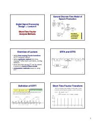
<strong>General</strong> <strong>Synthesis</strong> Model<br />
unvoiced sound<br />
amplitude<br />
Rz ( ) = 1−<br />
z<br />
1<br />
α −<br />
Pitch Detection, Voiced/Unvoiced/Silence Detection, Ga<strong>in</strong> Estimation, Vocal Tract<br />
Lecture_5_2013 1<br />
2<br />
Parameter Estimation, Glottal Pulse Shape, Radiation Model<br />
Fundamental Assumptions<br />
• properties of the speech signal change relatively<br />
slowly with time (5-10 sounds per second)<br />
– over very short (5-20 msec) <strong>in</strong>tervals => uncerta<strong>in</strong>ty<br />
due to small amount of data, vary<strong>in</strong>g pitch, vary<strong>in</strong>g<br />
amplitude<br />
– over medium length (20-100 msec) <strong>in</strong>tervals =><br />
uncerta<strong>in</strong>ty due to changes <strong>in</strong> sound quality,<br />
transitions between sounds, rapid transients <strong>in</strong><br />
speech<br />
– over long (100-500 msec) <strong>in</strong>tervals => uncerta<strong>in</strong>ty<br />
due to large amount of sound changes<br />
• there is always uncerta<strong>in</strong>ty <strong>in</strong> short time<br />
measurements and estimates from speech<br />
3<br />
signals<br />
Frame-by-Frame Process<strong>in</strong>g<br />
<strong>in</strong> Successive W<strong>in</strong>dows<br />
Frame 1<br />
Frame 2<br />
Frame 3<br />
Frame 4<br />
Frame 5<br />
75% frame overlap => frame length=L, frame shift=R=L/4<br />
Frame1={x[0],x[1],…,x[L-1]}<br />
Frame2={x[R],x[R+1],…,x[R+L-1]}<br />
Frame3={x[2R],x[2R+1],…,x[2R+L-1]}<br />
…<br />
5<br />
T 1<br />
T 2<br />
voiced sound<br />
amplitude<br />
Log Areas, Reflection<br />
Coefficients, Formants, Vocal<br />
Tract Polynomial, Articulatory<br />
Parameters, …<br />
Compromise Solution<br />
• “short-time” process<strong>in</strong>g methods => short segments of<br />
the speech signal are “isolated” and “processed” as if<br />
they were short segments from a “susta<strong>in</strong>ed” sound with<br />
fixed (non-time-vary<strong>in</strong>g) properties<br />
– this short-time process<strong>in</strong>g is periodically repeated for the<br />
duration of the waveform<br />
– these short analysis segments, or “analysis frames” often<br />
overlap one another<br />
– the results of short-time process<strong>in</strong>g can be a s<strong>in</strong>gle number (e.g.,<br />
an estimate of the pitch period with<strong>in</strong> the frame), or a set of<br />
numbers (an estimate of the formant frequencies for the analysis<br />
frame)<br />
– the end result of the process<strong>in</strong>g is a new, time-vary<strong>in</strong>g sequence<br />
that serves as a new representation of the speech signal<br />
Frame 1: samples 0,1,..., L −1<br />
Frame 2: samples RR , + 1,..., R+ L−1<br />
Frame 3: samples 2 R,2R+ 1,...,2 R+ L−1<br />
Frame 4: samples 3 R,3R+ 1,...,3 R+ L−1<br />
4<br />
1
Frame-by-Frame Process<strong>in</strong>g <strong>in</strong> Successive W<strong>in</strong>dows<br />
• <strong>Speech</strong> is processed frame-by-frame <strong>in</strong> overlapp<strong>in</strong>g <strong>in</strong>tervals until entire<br />
region of speech is covered by at least one such frame<br />
• Results of analysis of <strong>in</strong>dividual frames used to derive model parameters <strong>in</strong><br />
some manner<br />
• Representation goes from time sample x[<br />
n],<br />
n = , 0,<br />
1,<br />
2,<br />
to parameter<br />
vector f[ nˆ], n= ˆ 0,1,2, where n is the time <strong>in</strong>dex and ˆn is the frame <strong>in</strong>dex.<br />
Generic Short-<strong>Time</strong> Process<strong>in</strong>g<br />
x[n] T(x[n])<br />
T( ) w[n]<br />
Q<br />
∞ ⎛ ⎞<br />
Qnˆ= ⎜ ∑ T([ x m]) w[ n−m] ⎟<br />
⎝ ⎠<br />
l<strong>in</strong>ear or non-l<strong>in</strong>ear<br />
transformation<br />
m=−∞ n= nˆ<br />
w<strong>in</strong>dow sequence<br />
(usually f<strong>in</strong>ite length)<br />
Qˆn<br />
• ˆn is a sequence of local weighted average<br />
values of the sequence T(x[n]) at time n= nˆ<br />
Computation of Short-<strong>Time</strong> Energy<br />
• w<strong>in</strong>dow jumps/slides across sequence of squared values, select<strong>in</strong>g <strong>in</strong>terval<br />
for process<strong>in</strong>g<br />
• what happens to Eˆn<br />
as sequence jumps by 2,4,8,...,L samples ( E ˆn is a lowpass<br />
function—so it can be decimated without lost of <strong>in</strong>formation; why is E ˆn lowpass?)<br />
• effects of decimation depend on L; if L is small, then E ˆn is a lot more variable<br />
than if L is large (w<strong>in</strong>dow bandwidth changes with L!)<br />
11<br />
7<br />
9<br />
Short-<strong>Time</strong> Signal Process<strong>in</strong>g<br />
Short-<strong>Time</strong> Parameter<br />
s[ n] Analysis Qˆn<br />
Estimation f [ nˆ<br />
]<br />
speech<br />
waveform<br />
alternate<br />
representation<br />
model<br />
parameter(s)<br />
Model Parameter(s):<br />
• speech/non-speech<br />
• voiced/unvoiced/background<br />
• pitch period (when voiced)<br />
• formants<br />
Short-<strong>Time</strong> Energy<br />
∞<br />
2<br />
E = ∑ x m<br />
m=−∞<br />
[ ]<br />
-- this is the long term def<strong>in</strong>ition of signal energy<br />
-- there is little or no utility of this def<strong>in</strong>ition for time-vary<strong>in</strong>g signals<br />
2 2<br />
[ ] = x [ nˆ − L+ 1]<br />
+ ... + x [ nˆ]<br />
Enˆ= ∑<br />
m=<br />
− + 1<br />
2<br />
x m<br />
ˆ n<br />
nˆ L<br />
-- short-time energy <strong>in</strong> vic<strong>in</strong>ity of time nˆ<br />
T( x) = x<br />
2<br />
wn [ ] = 1 0≤n≤L−1 = 0 otherwise<br />
Effects of W<strong>in</strong>dow<br />
Q = T( x[ n]) ∗w[<br />
n]<br />
= x′ [ n] ∗w[<br />
n]<br />
nˆ n= nˆ<br />
n= nˆ<br />
• w[n] serves as a lowpass filter on T(x[n]) which often has a lot of<br />
high frequencies (most non-l<strong>in</strong>earities <strong>in</strong>troduce significant high<br />
frequency energy—th<strong>in</strong>k of what (x[n] x[n]) does <strong>in</strong> frequency)<br />
• often we extend the def<strong>in</strong>ition of Qˆn<br />
to <strong>in</strong>clude a pre-filter<strong>in</strong>g term<br />
so that x[n] itself is filtered to a region of <strong>in</strong>terest<br />
xˆ[ n] L<strong>in</strong>ear x[n]<br />
T(x[n])<br />
Lowpass ˆn<br />
T( )<br />
Filter<br />
Filter, w[n]<br />
Q<br />
8<br />
10<br />
12<br />
2
Short-<strong>Time</strong> Energy<br />
• serves to differentiate voiced and unvoiced sounds <strong>in</strong> speech<br />
from silence (background signal)<br />
• natural def<strong>in</strong>ition of energy of weighted signal is:<br />
∞<br />
∑<br />
∞<br />
nˆ<br />
= ∑<br />
2 2 ˆ −<br />
∞<br />
= ∑<br />
2 ˆ −<br />
m=−∞<br />
2<br />
m=−∞<br />
2<br />
Enˆ= ⎡⎣x[ m] w[ nˆ−m] ⎤⎦<br />
(sum of squares of portion of signal)<br />
m=−∞<br />
-- concentrates measurement at sample nˆ, us<strong>in</strong>g weight<strong>in</strong>g w[ n-m ˆ ]<br />
E x [ m] w [ n m] x [ m] h[ n m]<br />
hn [ ] = w [ n]<br />
x[n] x2 [n] Enˆ − short-time energy<br />
( ) 2 h[n]<br />
W<strong>in</strong>dows<br />
• consider two w<strong>in</strong>dows, w[n]<br />
– rectangular w<strong>in</strong>dow:<br />
• h[n]=1, 0≤n≤L-1 and 0 otherwise<br />
– Hamm<strong>in</strong>g w<strong>in</strong>dow (raised cos<strong>in</strong>e w<strong>in</strong>dow):<br />
• h[n]=0.54-0.46 cos(2πn/(L-1)), 0≤n≤L-1 and 0 otherwise<br />
– rectangular w<strong>in</strong>dow gives equal weight to all L<br />
samples <strong>in</strong> the w<strong>in</strong>dow (n,...,n-L+1)<br />
– Hamm<strong>in</strong>g w<strong>in</strong>dow gives most weight to middle<br />
samples and tapers off strongly at the beg<strong>in</strong>n<strong>in</strong>g and<br />
the end of the w<strong>in</strong>dow<br />
W<strong>in</strong>dow Frequency Responses<br />
• rectangular w<strong>in</strong>dow<br />
s<strong>in</strong>( ΩLT<br />
/ 2)<br />
He ( ) =<br />
e<br />
s<strong>in</strong>( ΩT<br />
/ 2)<br />
jΩT −jΩT( L−1)/<br />
2<br />
• first zero occurs at f=Fs/L=1/(LT) (or Ω=(2π)/(LT)) =><br />
nom<strong>in</strong>al cutoff frequency of the equivalent “lowpass” filter<br />
• Hamm<strong>in</strong>g w<strong>in</strong>dow<br />
wH[ n] = 0.54 wR[ n] −0.46*cos(2 π n/ ( L−1)) wR[ n]<br />
• can decompose Hamm<strong>in</strong>g W<strong>in</strong>dow FR <strong>in</strong>to comb<strong>in</strong>ation<br />
of three terms<br />
13<br />
15<br />
17<br />
Short-<strong>Time</strong> Energy Properties<br />
• depends on choice of h[n], or equivalently,<br />
w<strong>in</strong>dow w[n]<br />
–if w[n] duration very long and constant amplitude<br />
(w[n]=1, n=0,1,...,L-1), E ˆn would not change much over<br />
time, and would not reflect the short-time amplitudes of<br />
the sounds of the speech<br />
– very long duration w<strong>in</strong>dows correspond to narrowband<br />
lowpass filters<br />
– want E ˆn to change at a rate comparable to the chang<strong>in</strong>g<br />
sounds of the speech => this is the essential conflict <strong>in</strong><br />
all speech process<strong>in</strong>g, namely we need short duration<br />
w<strong>in</strong>dow to be responsive to rapid sound changes, but<br />
short w<strong>in</strong>dows will not provide sufficient averag<strong>in</strong>g to<br />
give smooth and reliable energy function<br />
Rectangular and Hamm<strong>in</strong>g W<strong>in</strong>dows<br />
<strong>Time</strong> Responses of L=21 po<strong>in</strong>t Rectangular and<br />
Hamm<strong>in</strong>g w<strong>in</strong>dows; Frequency Responses of L=51<br />
po<strong>in</strong>t Rectangular and Hamm<strong>in</strong>g W<strong>in</strong>dows<br />
W<strong>in</strong>dow Frequency Responses<br />
Rectangular W<strong>in</strong>dows,<br />
L=21,41,61,81,101<br />
Hamm<strong>in</strong>g W<strong>in</strong>dows,<br />
L=21,41,61,81,101<br />
14<br />
16<br />
18<br />
3
RW and HW Frequency Responses<br />
•bandwidth of HW is approximately twice the bandwidth of RW<br />
• attenuation of more than 40 dB for HW outside passband,<br />
versus 14 dB for RW<br />
• stopband attenuation is essentially <strong>in</strong>dependent of L, the<br />
w<strong>in</strong>dow duration => <strong>in</strong>creas<strong>in</strong>g L simply decreases w<strong>in</strong>dow<br />
bandwidth<br />
• L needs to be larger than a pitch period (or severe<br />
fluctuations will occur <strong>in</strong> En), but smaller than a sound duration<br />
(or En will not adequately reflect the changes <strong>in</strong> the speech<br />
signal)<br />
There is no perfect value of L, s<strong>in</strong>ce a pitch period can be as short as 20 samples (500 Hz at a 10 kHz<br />
sampl<strong>in</strong>g rate) for a high pitch child or female, and up to 250 samples (40 Hz pitch at a 10 kHz sampl<strong>in</strong>g<br />
rate) for a low pitch male; a compromise value of L on the order of 100-200 samples for a 10 kHz sampl<strong>in</strong>g<br />
rate is often used <strong>in</strong> practice<br />
Short-<strong>Time</strong> Energy us<strong>in</strong>g RW/HW<br />
E ˆn<br />
ˆn<br />
L=51<br />
L=51<br />
E<br />
L=101<br />
L=201<br />
L=401<br />
•as L <strong>in</strong>creases, the plots tend to converge (however you are smooth<strong>in</strong>g sound energies)<br />
• short-time energy provides the basis for dist<strong>in</strong>guish<strong>in</strong>g voiced from unvoiced speech<br />
regions, and for medium-to-high SNR record<strong>in</strong>gs, can even be used to f<strong>in</strong>d regions of 21<br />
silence/background signal<br />
19<br />
L=101<br />
L=201<br />
L=401<br />
Recursive Short-<strong>Time</strong> Energy<br />
i un [ −m−1] implies the condition n−m−1≥0 or m ≤n−1giv<strong>in</strong>g 2<br />
n−1<br />
∑<br />
m=−∞<br />
2 n−m−1 2 2<br />
σ [ n] = ( 1− α) x [ m] α = ( 1−α)( x [ n− 1] + αx<br />
[ n−<br />
2]<br />
+ ...)<br />
i for the <strong>in</strong>dex n −1<br />
we have<br />
2<br />
n−2<br />
∑<br />
m=−∞<br />
2 n−m−2 2 2<br />
σ [ n− 1] = ( 1− α) x [ m] α = ( 1−α)( x [ n− 2] + αx<br />
[ n−<br />
3]<br />
+ ...)<br />
i thus giv<strong>in</strong>g the relationship<br />
2 2 2<br />
σ [ n] = α ⋅σ [ n− 1] + x [ n−1](<br />
1−α)<br />
i and def<strong>in</strong>es an Automatic Ga<strong>in</strong> Control (AGC) of the form<br />
G0<br />
Gn [ ] =<br />
σ [ n]<br />
23<br />
W<strong>in</strong>dow Comparisons<br />
Short-<strong>Time</strong> Energy for AGC<br />
Can use an IIR filter to def<strong>in</strong>e short-time energy, e.g.,<br />
• time-dependent energy def<strong>in</strong>ition<br />
2<br />
∞<br />
= ∑<br />
2<br />
−<br />
∞<br />
∑<br />
m=−∞ m=<br />
0<br />
σ [ n] x [ m] h[ n m]/ h[ m]<br />
• consider impulse response of filter of form<br />
n−1 n−1<br />
hn [ ] = α un [ − 1] = α n≥1<br />
= 0 n < 1<br />
2<br />
∞<br />
∑<br />
m=−∞<br />
2 n−m−1 σ [ n] = ( 1−α) x [ m] α u[ n−m−1] Alternative AGC Derivation<br />
2 2<br />
σ [ n] = x [ n] ∗h[<br />
n]<br />
n−1<br />
hn [ ] = (1 −α) α un [ −1]<br />
i Make the substitutions of variables:<br />
2<br />
yn [ ] = σ [ n]<br />
2<br />
xn [<br />
] = x [ n]<br />
i giv<strong>in</strong>g:<br />
Yz ( ) = Xz ( ) ⋅Hz<br />
( )<br />
i Solv<strong>in</strong>g for Hz ( ) and plugg<strong>in</strong>g <strong>in</strong> gives:<br />
∞<br />
−1<br />
n−1−n ( 1−<br />
α ) z<br />
Hz ( ) = (1 − α) ∑α<br />
z =<br />
−1<br />
n=<br />
1 1−<br />
αz<br />
−1<br />
Yz ( ) = X<br />
( 1−<br />
α ) z<br />
( z)<br />
−1<br />
1−<br />
αz<br />
−1 −1<br />
Yz ( ) − αzYz ( ) = Xz ( ) ( 1−α)<br />
z<br />
i Transform<strong>in</strong>g gives:<br />
yn [ ] = αyn [ − 1] + xn [<br />
−1] ( 1−α)<br />
2 2 2<br />
σ [ n] = ασ [ n− 1] + x [ n−1](1<br />
−α)<br />
20<br />
22<br />
24<br />
4
Recursive Short-<strong>Time</strong> Energy<br />
x [n]<br />
(<br />
2<br />
)<br />
2<br />
x [ n]<br />
1<br />
z<br />
( 1−<br />
α)<br />
+<br />
2<br />
σ [ n]<br />
−<br />
1<br />
z −<br />
α<br />
2 2 2<br />
σ [ n] = α ⋅σ [ n− 1] + x [ n−1](<br />
1−α)<br />
Use of Short-<strong>Time</strong> Energy for AGC<br />
Short-<strong>Time</strong> Magnitude<br />
• short-time energy is very sensitive to large<br />
signal levels due to x2 [n] terms<br />
– consider a new def<strong>in</strong>ition of ‘pseudo-energy’ based<br />
on average signal magnitude (rather than energy)<br />
∞<br />
M = | xm [ ]| wn [ ˆ −m]<br />
nˆ<br />
m=−∞<br />
– weighted sum of magnitudes, rather than weighted<br />
sum of squares<br />
x[n]<br />
∑<br />
|x[n]|<br />
| | w[n]<br />
M = M =<br />
nˆ n n nˆ<br />
• computation avoids multiplications of signal with itself (the squared term)<br />
25<br />
27<br />
29<br />
Recursive Short-<strong>Time</strong> Energy<br />
Use of Short-<strong>Time</strong> Energy for AGC<br />
α = 0.9<br />
α = 0.99<br />
Short-<strong>Time</strong> Magnitudes<br />
• differences between En and Mn noticeable <strong>in</strong> unvoiced regions<br />
• dynamic range of Mn ~ square root (dynamic range of En) => level differences between voiced and<br />
unvoiced segments are smaller<br />
• En and Mn can be sampled at a rate of 100/sec for w<strong>in</strong>dow durations of 20 msec or so => efficient 30<br />
representation of signal energy/magnitude<br />
M<br />
M ˆn<br />
ˆn<br />
L=51 L=51<br />
L=101 L=101<br />
L=201 L=201<br />
L=401 L=401<br />
26<br />
28<br />
5
Short <strong>Time</strong> Energy and Magnitude—<br />
Rectangular W<strong>in</strong>dow<br />
E ˆn<br />
L=51 L=51<br />
L=101<br />
L=201<br />
L=401<br />
M ˆn<br />
L=101<br />
L=201<br />
L=401<br />
Short-<strong>Time</strong> Average ZC Rate<br />
zero cross<strong>in</strong>gs<br />
zero cross<strong>in</strong>g => successive samples<br />
have different algebraic signs<br />
• zero cross<strong>in</strong>g rate is a simple measure of the ‘frequency content’ of a<br />
signal—especially true for narrowband signals (e.g., s<strong>in</strong>usoids)<br />
• s<strong>in</strong>usoid at frequency F0 with sampl<strong>in</strong>g rate FS has FS/F0 samples per<br />
cycle with two zero cross<strong>in</strong>gs per cycle, giv<strong>in</strong>g an average zero<br />
cross<strong>in</strong>g rate of<br />
z1=(2) cross<strong>in</strong>gs/cycle x (F0 / FS ) cycles/sample<br />
z1=2F0 / FS cross<strong>in</strong>gs/sample (i.e., z1 proportional to F0 )<br />
zM=M (2F0 /FS ) cross<strong>in</strong>gs/(M samples)<br />
S<strong>in</strong>usoid Zero Cross<strong>in</strong>g Rates<br />
Assume the sampl<strong>in</strong>g rate is FS<br />
= 10, 000 Hz<br />
1. F0 = 100 Hz s<strong>in</strong>usoid has FS/ F0<br />
= 10, 000 / 100 = 100 samples/cycle;<br />
or z1 = 2 / 100 cross<strong>in</strong>gs/sample, or z100<br />
= 2 / 100 * 100 =<br />
2 cross<strong>in</strong>gs/10 msec <strong>in</strong>terval<br />
2. F0 = 1000 Hz s<strong>in</strong>usoid<br />
has FS/ F0=<br />
10, 000 / 1000 = 10 samples/cycle;<br />
or z1 = 2 / 10 cross<strong>in</strong>gs/sample, or z100<br />
= 2 / 10 * 100 =<br />
20 cross<strong>in</strong>gs/10 msec <strong>in</strong>terval<br />
3. F0 = 5000 Hz s<strong>in</strong>usoid has FS/ F0<br />
= 10, 000 / 5000 = 2 samples/cycle;<br />
or z1 = 2/ 2 cross<strong>in</strong>gs/sample,<br />
or z100<br />
= 2/ 2* 100=<br />
100 cross<strong>in</strong>gs/10 msec <strong>in</strong>terval<br />
31<br />
33<br />
35<br />
Short <strong>Time</strong> Energy and Magnitude—Hamm<strong>in</strong>g<br />
W<strong>in</strong>dow<br />
E ˆn<br />
L=51<br />
L=101<br />
L=201<br />
L=401<br />
M ˆn<br />
L=51<br />
L=101<br />
L=201<br />
L=401<br />
Short-<strong>Time</strong> Average ZC Rate<br />
Zero Cross<strong>in</strong>g for S<strong>in</strong>usoids<br />
1<br />
0.5<br />
0<br />
-0.5<br />
-1<br />
0 50 100 150 200<br />
1.5<br />
1<br />
0.5<br />
0<br />
offset:0.75, 100 Hz s<strong>in</strong>ewave, ZC:9, offset s<strong>in</strong>ewave, ZC:8<br />
Offset=0.75<br />
0 50 100 150 200<br />
100 Hz s<strong>in</strong>ewave<br />
100 Hz s<strong>in</strong>ewave with dc offset<br />
32<br />
34<br />
ZC=9<br />
ZC=8<br />
36<br />
6
Zero Cross<strong>in</strong>gs for Noise<br />
3<br />
2<br />
1<br />
0<br />
-1<br />
-2<br />
6<br />
4<br />
2<br />
0<br />
offseet:0.75, random noise, ZC:252, offset noise, ZC:122<br />
0 50 100 150 200<br />
Offset=0.75<br />
random gaussian noise<br />
random gaussian noise with dc offset<br />
-2<br />
0 50 100 150 200 250<br />
1<br />
ZC Normalization<br />
i The formal def<strong>in</strong>ition of zn<br />
is:<br />
Z<br />
1<br />
= z =<br />
nˆ<br />
| sgn( xm [ ]) −sgn( xm [ −1])<br />
|<br />
nˆ<br />
∑<br />
2 L m= nˆ− L+<br />
1<br />
is <strong>in</strong>terpreted as the number of zero cross<strong>in</strong>gs per sample.<br />
ZC=252<br />
ZC=122<br />
i For most practical applications, we need the rate of zero cross<strong>in</strong>gs<br />
per fixed <strong>in</strong>terval of M samples, which is<br />
zM= z1⋅ M = rate of zero cross<strong>in</strong>gs per M sample <strong>in</strong>terval<br />
Thus, for an <strong>in</strong>terval of τ sec., correspond<strong>in</strong>g to M samples we get<br />
z = z ⋅ M; M = τ F = τ /T<br />
M 1<br />
S<br />
ZC Rate Distributions<br />
1 KHz 2KHz 3KHz 4KHz<br />
• for voiced speech, energy is ma<strong>in</strong>ly below 1.5 kHz<br />
• for unvoiced speech, energy is ma<strong>in</strong>ly above 1.5 kHz<br />
• mean ZC rate for unvoiced speech is 49 per 10 msec <strong>in</strong>terval<br />
• mean ZC rate for voiced speech is 14 per 10 msec <strong>in</strong>terval<br />
Unvoiced <strong>Speech</strong>:<br />
the dom<strong>in</strong>ant energy<br />
component is at<br />
about 2.5 kHz<br />
Voiced <strong>Speech</strong>: the<br />
dom<strong>in</strong>ant energy<br />
component is at<br />
about 700 Hz<br />
37<br />
39<br />
41<br />
ZC Rate Def<strong>in</strong>itions<br />
∞ 1<br />
Z = ∑<br />
− −1ˆ nˆ<br />
| sgn( x[ m]) sgn( x[ m ]) | w[ n−m] 2Leff<br />
m=−∞<br />
sgn( xn [ ]) = 1 xn [ ] ≥ 0<br />
=− 1 xn [ ] < 0<br />
i simple w<strong>in</strong>dow, rectangular with<br />
wn [ ] = 1 0≤n≤L−1 = 0 otherwise<br />
i L = L<br />
eff<br />
same form for Z n as for E n or M n<br />
ZC Normalization<br />
i For a 1000 Hz s<strong>in</strong>ewave as <strong>in</strong>put, us<strong>in</strong>g a 40 msec w<strong>in</strong>dow length<br />
( L), with various values of sampl<strong>in</strong>g rate ( F ), we get the follow<strong>in</strong>g:<br />
F L z M z<br />
S 1<br />
M<br />
8000 320 1/ 4 80 20<br />
10000 400 1/ 5 100 20<br />
16000 640 1/ 8 160 20<br />
i Thus we see<br />
that the normalized (per <strong>in</strong>terval) zero cross<strong>in</strong>g rate,<br />
zM,<br />
is <strong>in</strong>dependent of the sampl<strong>in</strong>g rate and can be used as a measure<br />
of the dom<strong>in</strong>ant energy <strong>in</strong> a band.<br />
ZC Rates for <strong>Speech</strong><br />
S<br />
38<br />
40<br />
• 15 msec w<strong>in</strong>dows<br />
• 100/sec sampl<strong>in</strong>g<br />
rate on ZC<br />
computation<br />
42<br />
7
Short-<strong>Time</strong> Energy, Magnitude, ZC<br />
Summary of Simple <strong>Time</strong> <strong>Doma<strong>in</strong></strong><br />
Measures<br />
xˆ ( n)<br />
L<strong>in</strong>ear x(n) T[x(n)] Lowpass ˆn<br />
T[ ]<br />
Filter<br />
Filter, w(n)<br />
∞<br />
∑<br />
Qnˆ= T( x[ m]) w[ nˆ−m] m=−∞<br />
1. Energy:<br />
Enˆ= nˆ<br />
∑<br />
m= nˆ− L+<br />
1<br />
2<br />
x [ m] w[ nˆ−m] i can downsample Enˆ<br />
at rate commensurate with w<strong>in</strong>dow bandwidth<br />
2. Magnitude:<br />
Mnˆ= nˆ<br />
∑<br />
m= nˆ− L+<br />
1<br />
x[ m] w[ nˆ−m] 3. Zero Cross<strong>in</strong>g Rate:<br />
1<br />
Znˆ= z1= ∑ sgn( x − −<br />
2L<br />
= − +<br />
= ≥<br />
=− <<br />
ˆ n<br />
[ m]) sgn( x[ m 1])<br />
m nˆ L 1<br />
where sgn( xm [ ]) 1 xm [ ] 0<br />
1 xm [ ] 0<br />
Periodic Signals<br />
• for a periodic signal we have (at least <strong>in</strong><br />
theory) Φ[P]=Φ[0] so the period of a<br />
periodic signal can be estimated as the<br />
first non-zero maximum of Φ[k]<br />
– this means that the autocorrelation function is<br />
a good candidate for speech pitch detection<br />
algorithms<br />
– it also means that we need a good way of<br />
measur<strong>in</strong>g the short-time autocorrelation<br />
function for speech signals<br />
Q<br />
Issues <strong>in</strong> ZC Rate Computation<br />
• for zero cross<strong>in</strong>g rate to be accurate, need zero<br />
DC <strong>in</strong> signal => need to remove offsets, hum,<br />
noise => use bandpass filter to elim<strong>in</strong>ate DC and<br />
hum<br />
• can quantize the signal to 1-bit for computation<br />
of ZC rate<br />
• can apply the concept of ZC rate to bandpass<br />
filtered speech to give a ‘crude’ spectral estimate<br />
<strong>in</strong> narrow bands of speech (k<strong>in</strong>d of gives an<br />
estimate of the strongest frequency <strong>in</strong> each<br />
narrow band of speech)<br />
43 44<br />
45<br />
47<br />
Short-<strong>Time</strong> Autocorrelation<br />
-for a determ<strong>in</strong>istic signal, the autocorrelation function is def<strong>in</strong>ed as:<br />
∞<br />
∑<br />
Φ[ k] = x[ m] x[ m+ k]<br />
m=−∞<br />
-for a random or periodic signal, the autocorrelation function is:<br />
L 1<br />
Φ[ k] = lim ∑ x[ m] x[ m+ k]<br />
N→∞<br />
( 2L+ 1)<br />
m=−L - if x[<br />
n] = x[ n+ P], then Φ[ k] = Φ[ k + P],<br />
=> the autocorrelation function<br />
preserves periodicity<br />
-properties of Φ[ k]<br />
:<br />
1.<br />
Φ[ k] is even, Φ[ k] = Φ[ −k]<br />
2. Φ[ k] is maximum at k = 0, | Φ[ k] | ≤Φ[ 0],<br />
∀k<br />
3. Φ[ 0]<br />
is the signal energy or power<br />
(for random signals)<br />
Short-<strong>Time</strong> Autocorrelation<br />
- a reasonable def<strong>in</strong>ition for the short-time autocorrelation is:<br />
∞<br />
R ˆ ˆ<br />
nˆ<br />
[ k] = ∑ x[ mw ] [ n− m] x[ m+ k] w[ n−k −m]<br />
m=−∞<br />
1. select a segment of speech by w<strong>in</strong>dow<strong>in</strong>g<br />
2. compute determ<strong>in</strong>istic autocorrelation of the w<strong>in</strong>dowed speech<br />
Rnˆ[ k] = Rnˆ[ −k]<br />
- symmetry<br />
∞<br />
= ∑ xmxm [ ] [ −k] ⎡⎣wn [ ˆ− mwn ] [ ˆ+<br />
k−m] ⎤⎦<br />
m=−∞<br />
- def<strong>in</strong>e filter of the form<br />
h [ ˆ] = [ ˆ] [ ˆ<br />
k n w n w n+ k]<br />
- this enables us to write the short-time autocorrelation <strong>in</strong> the form:<br />
∞<br />
R ˆ<br />
nˆ<br />
[ k] = ∑ xmxm [ ] [ −k] hk[ n−m] m=−∞<br />
th<br />
- the value of R ˆ<br />
nˆ<br />
[ k] at time n for the k lag is obta<strong>in</strong>ed by filter<strong>in</strong>g<br />
the sequence xn [ ˆ] xn [ ˆ − k] with a filter with impulse<br />
response h [ ˆ k n]<br />
46<br />
48<br />
8
Short-<strong>Time</strong> Autocorrelation<br />
∞<br />
∑ [ ][ ]<br />
R[ k] = xmwn [ ] [ − m] xm [ + kwn ] [ −k−m] n<br />
m=−∞<br />
L−− 1 k<br />
∑ [ ′ ][ ′ ]<br />
R [ k] = x[ n+ mw ] [ m] x[ n+ m+ k] w [ k + m]<br />
n<br />
m=<br />
0<br />
n-L+1 n+k-L+1<br />
⇒ L−k po<strong>in</strong>ts used to compute R [ k]<br />
• autocorrelation peaks occur at k=72, 144, ... => 140 Hz<br />
pitch<br />
• Φ(P)
Unvoiced L=401<br />
Effects of W<strong>in</strong>dow Size<br />
L=401<br />
L=251<br />
L=125<br />
55<br />
• choice of L, w<strong>in</strong>dow duration<br />
• small L so pitch period<br />
almost constant <strong>in</strong> w<strong>in</strong>dow<br />
• large L so clear<br />
periodicity seen <strong>in</strong> w<strong>in</strong>dow<br />
• as k <strong>in</strong>creases, the<br />
number of w<strong>in</strong>dow po<strong>in</strong>ts<br />
decrease, reduc<strong>in</strong>g the<br />
accuracy and size of Rn(k) for large k => have a taper<br />
of the type R(k)=1-k/L, |k|
Examples of Modified AC<br />
L=401<br />
L=401<br />
L=401<br />
Modified Autocorrelations –<br />
fixed value of L=401<br />
Summary<br />
Modified Autocorrelations –<br />
values of L=401,251,125<br />
• short-time analysis of speech signals<br />
– short-time energy (short-time log energy)<br />
– short-time average magnitude<br />
– short-time zero cross<strong>in</strong>g rate<br />
– short-time autocorrelation<br />
– modified short-time autocorrelation<br />
L=401<br />
L=251<br />
L=125<br />
61<br />
63<br />
Autocorrelations<br />
62<br />
11