vibration fatigue analysis of a cantilever beam using different fatigue ...

VIBRATION FATIGUE ANALYSIS OF A CANTILEVER BEAM USING
ABSTRACT
DIFFERENT FATIGUE THEORIES
Yusuf ELDOĞAN †‡ , Ender CIGEROGLU †
† Middle East Technical University, 06800, Ankara, Turkey
‡ ASELSAN MGEO Inc., 06750, Ankara, Turkey
In this study, vibration fatigue analysis of a cantilever beam is performed using an in-house numerical code. Finite
element model (FEM) of the cantilever beam verified by tests is used for the analysis. Several vibration fatigue
theories are used to obtain fatigue life of the cantilever beam for white noise random input and the results
obtained are compared with each other. Fatigue life calculations are repeated for different damping ratios and the
effect of damping ratio is studied. Moreover, using strain data obtained from cantilever beam experiments, fatigue
life of the beam is determined by utilizing time domain (Rainflow counting method) and frequency domain
methods, which are compared with each other. In addition to this, fatigue tests are performed on cantilever beam
specimens and fatigue life results obtained experimentally are compared with that of in-house numerical code. It
is observed that the accuracy of the damping ratio is very important for accurate determination of fatigue life.
Furthermore, for the case considered, it is observed that the fatigue life result obtained from Dirlik method is
considerably similar to that of Rainflow counting method.
Keywords: Vibration Fatigue Theories, Rainflow Counting, Dirlik Method, Probability Density Function,
Frequency Domain Fatigue Theories
INTRODUCTION
In vibration environments, if structures are designed only considering static requirements, due to dynamic
characteristic of the environment, generally failure occurs. Hence, in order to avoid this kind of failures, dynamic
characteristic of the environment and the structure should be considered. If the loading is cyclic, usually such
failures occur even though stresses caused by these cyclic loadings are smaller than yield or ultimate strength of
the material. These kinds of failures caused by cyclic loadings are called "Fatigue". However, especially in
military environments, generally structures are exposed to random loading; hence, the resulting stresses are not

cyclic. In order to avoid fatigue due to random loading, fatigue life of structures should be calculated using
vibration fatigue approaches in time and frequency domains.
In the following sections, firstly, brief information about vibration fatigue approaches used in this study is
described. These fatigue life estimation approaches are employed in order to determine the fatigue life of an
example cantilever beam. In addition to this, fatigue life of the cantilever beam is determined experimentally, by
utilizing several cantilever beams and an average fatigue life is determined. The results obtained from different
fatigue approaches are compared with each other and also with the experimental data.
THEORY
In frequency domain, expected fatigue damage, ED , caused by random loading is given as follows[1];
n
ED . (1)
N
where, n and N are the number of stress cycles applied at a fixed stress amplitude and the number of cycles the
material can withstand at applied fixed stress amplitude, respectively.
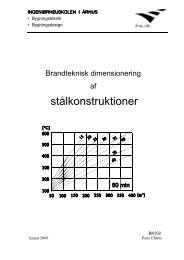
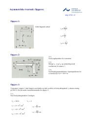
In order to calculate ED, firstly Probability Density Function (PDF), p S , of rainflow stress ranges should be
determined. A typical PDF is shown in Fig. 1 [2].
Fig. 1 Probability Density Function (PDF)
The bin widths, dS and total number of cycles in the histogram, S t should be obtained in order to calculate PDF
from a stress range histogram. The opposite work can also be performed using PDF. The area shown in Fig. 1,
p S dS,
gives the probability of stress ranges between
widths.
p(S)
dS
Stress (S)
dS dS
Si and Si where i indicates the number of bin
2
2
Finally, multiplying the probability of stress ranges with the total number of cycles, S t , in the histogram, the
number of total cycles, nS , for a given stress level, S , can be obtained as follows [2]:

n( S) p( S) dS St
. (2)
In order to use Eq. (1), nS is obtained from PDF. For a given stress level, S , total number of cycles, NS ,
which cause failure, can be obtained by using Wohler curve formulation, which is defined as :
b
N C S
. (3)
In Eq. (3), b is Basquin exponent and C is a material constant.
Finally, by substituting Eq. (2) and Eq. (3) into Eq. (1), expected fatigue damage, ED, can be found as:
niS St
b
NS C
. (4)
E D S p S dS
i
i
0
In frequency domain, Power Spectral Density (PSD) obtained from random time histories is the most widely used
expression for the calculation of fatigue life if vibration fatigue theory is used [3].
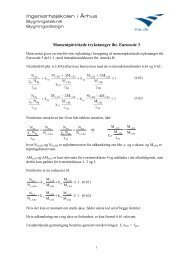
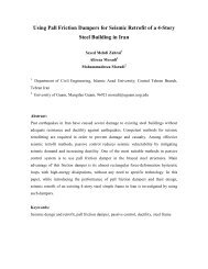
There are many different techniques that determine the PDF as functions of four spectral moments of the PSD
( m0, m1, m2, m 4).These
spectral moments of the PSD given in Fig. 2 are expressed as G
k f
k [1]
m
m
n
n
0
G f df f
k
G k f
k f
, (5)
k 1
where f , G
k f
k
and f are frequency, PSD and frequency increment, respectively.
Fig. 2 Power Spectral Density of Stress
In 1954, a very important relationship is developed by S.O Rice [4], for the number of upward mean crossings per
second, EP , and peaks per second, E 0 , in terms of the spectral moments defined by Eq. (5) in a random
signal. The relationships developed by Rice can be given as follows;
m m
E P E
, 0
2
Stress
Hz
4 2
. (6)
m2 m0
By utilizing Eq. (6), irregularity factor can be defined as
f k
Gk ⋅ fk
Frequency Hz

0
2
2
E m
E P m m
0 4
. (7)
Theoretically, this factor can only take a value in the range of 0 to 1. If the value is 1, the process is narrow band
otherwise; it tends to be white noise. It should be noted that;
EPT St,
(8)
where, T is fatigue life in seconds.
By substituting Eq. (8) into Eq. (4), expected damage formulation is obtained as
niS EPT b
NS C , (9)
E D S p S dS
i
i
0
which can be used in frequency domain applications. By setting ED equal to 1, fatigue life, T , can be obtained.
However, it is worth noting that, while calculating fatigue damage by using Eq. (9), an appropriate cut-off value
should be used for the upper limit of integration.
Bendat [5] first proposed a frequency domain solution, which gives conservative results for wide-band
applications. Therefore, Bendat’s solution is also called as a Narrow-Band solution. As a result of this, for
Narrow-Band solution, probability density function and expected damage are given as follows:
S
pS e
4 m
NB
0
S
2
8m0 , (10)
2
S
niS EPT b S 8m0 NS C . (11)
4
m
E D S e dS
i
i
0
0
In order to solve the problem of getting conservative results from narrow-band solutions, many expressions are
investigated. The first expression for expected damage developed by Wirsching [6] is
c
1 1
E D E D a a , (12)
NB
where, ED is the expected damage determined by narrow-band solutions and
NB
a 0.926 0.033b,
c 1.587b 2.323,
2
1
. (13)
Later, Tunna [7] replaced the expression of probability density function given in narrow-band solution with the
following one
S
pS e
4 m 0
S
2
8m0 . (14)

Expected fatigue damage, ED , given by Eq.(9) can be also described as follows
E P T
ED Seq
(14)
C
where, S eq is equivalent stress.
In order to find equivalent stress, Hancock [8] first proposed the following expression
b Seq 2 2m 1
Hancock
2
0
1
b
Chaudhuery and Dover [9] used a different expression for equivalent stress
1
b2 b
b b b
2 2 1 2 2
22 2 2 2 2
S m0 erf eq CandD
However, the simplest form of equivalent stress is given by Steinberg [10] as
b b b
1
b
S 0.6832 m0 0.2714 m0 0.0436 m0
eq Steinberg
(15)
. (16)
(17)
The best correlation in order to find probability density function is proposed by Dirlik [11] and it is given as
2
Z Z
Z
2
1 Q 22 R
2
e e D 2
2
3 Ze D D Z
pS ( )
Q R
2
m
where,
0
2 2
2( xm ) 1D1D1 1D1D2
1 ,
2 2 , 3
D D D
1
1R 1R
, (18)
.
Dirlik investigated this method without using narrow-band solution. This empirical closed form of PDF is
obtained by using computer simulations based on Monte Carlo technique [1].
RESULTS
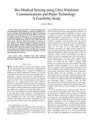
An Aluminum 6061 T6 beam shown in Fig. 3 is used for case studies, finite element model (FEM) of which is
verified by tests[12].

Case Study 1
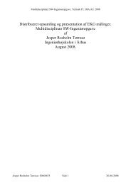
In this case study, fatigue analyses and tests are performed using the white noise PSD acceleration given in Fig. 4
as base input.
AMPLITUDE (g 2 /HZ)
0.18
0.16
0.14
0.12
0.1
0.08
0.06
0.04
0.02
0
411
350
Fig. 3 Dimensions of the Cantilever Beam
PSD INPUT
50 100 150 200 250 300 350 400 450 500
FREQUENCY (HZ)
Fig. 4 PSD Input Acceleration for Fatigue Analysis
Experimental setup is shown in Fig. 5 where the beam is fixed to shaker. Since the experimental setup is
configured perpendicular to gravity direction, there is no mean component of the stress can be neglected. The test
is stopped when the crack is observed and the time from the beginning to the end of the test is accepted to be the
fatigue life of the cantilever beam. The test is repeated for seven cantilever beams and the average of the results is
accepted as the fatigue life of the beam. The fatigue life results for the seven test items and average of them is
given in Table 1.
3
7
1.5
R 1.5
50

Fig. 5 Experi imental Setup p for Cantilevver
Beam Fatiigue
Test
Ta able 1 Fatigue e Life of Testt
Specimens
CONDITION
TE EST ITEM 1
TE EST ITEM 2
TE EST ITEM 3
TE EST ITEM 4
TE EST ITEM 5
TE EST ITEM 6
TE EST ITEM 7
AVE ERAGE LIF FE
FATIGGUE
LIFE (s) )
FFatigue
life of o cantilever beam is calculated
using different vibbration
fatiguue
theories ass
mentioned iin
Theory
ssection.
The obtained o fatig gue life results s together wit th experimenttally
obtainedd
fatigue life aare
given in TTable
2. It
ccan
be conclu uded from the e results obta ained that Dir rlik [11] methhod
generallyy
gives the mmost
accurate results of
ffatigue
life. In n addition, co omparison of f the location ns of crack innitiation
estimmated
from bboth
finite eleement
and
eexperimental
setup is show wn in Fig. 6, which w are in good g agreement
IIn
addition, in n order to obs serve how the e damping rat tio affects thee
fatigue life results of thee
cantilever bbeam,
four
ddifferent
fatig gue life analy yses are perf formed using 0.5%, 1%, 1.5% and 2% % constant ddamping
ratioos
and the
rresults
includi ing that of id dentified damp ping ratio are e given Tablee
3. It is observed
from thee
results that, , damping
rratio
of the st tructure affects
the fatigue e life significa antly. Hence, , accurate ideentification
off
the dampingg
ratios is
ccrucial
in the estimation of f fatigue life.
1320
1260
1250
1380
1200
1400
1200
1287

Table 2 Fa atigue Life of Cantilever Be eam Predicted d by Differennt
Vibration FFatigue
Theorries
and Experriments
MET THOD
NARROW-BAND
WIRC CHING
TUN NNA
HANC COCK
KAM and d DOVER
STEIN NBERG
DIR RLIK
EXPER RIMENT
Fi ig. 6 Location ns of the Crac ck Initiation for fo Both Finitee
Element andd
Manufacturred
Models
Table 3 Fati igue Life Resu ults of Cantilever
Beam foor
Three Diffeerent
Dampinng
Ratios
FATI IGUE THOR RIES
FREQUENCY
Y
DOMAIN
0.5 5%
DAM MPING
RAT TIO
FATIGUE
(s)
9.57E+0 01 1.59E+00
1.59E+0 02 22.65E+00
6.05E+0 02 1.01E+01
3.76E-0 03 66.27E-05
3.76E-0 03 66.27E-05
3.76E-0 03 66.27E-05
9.84E+0 02 1.64E+01
1.29E+0 03 22.15E+01
1%
DAM MPING
RATIO R
NA ARROW-BAN ND 1.47E E+02 2.5 58E+02 44.13E+02
WIRCHING
W G 2.45E E+02 4.2 29E+02 66.87E+02
TUNNA 1.22E E+03 4.2 26E+03 11.08E+04
HANCOCK
H
5.04 4E-03 5.2 25E-03 55.35E-03
KAM M and DOV VER 5.04 4E-03 5.2 25E-03 55.35E-03
STEINBERG
S G 5.04 4E-03 5.2 25E-03 55.35E-03
DIRLIK 1.41E E+03 2.9 90E+03 55.00E+03
% DIFFERRENCE
LIFE FATIIGUE
LIFE
WITHH
(min)
EXPERIMEENTAL
FATIGGUE
LIFE ( (s)
1.5%
DDAMPING
RATIO
93
88
53
100
100
100
24
-
2%
DAMPING
RATIO
6.73E+02
1.12E+03
2.21E+04
6.60E+00
5.44E-03
5.44E-03
8.35E+03
IDENTIFIEED
DAMPINGG
RATIO
9.57E+01
1.59E+022
6.05E+022
3.76E-03
3.76E-03
3.76E-03
9.84E+022

Case Study 2
In this case study, firstly, rainflow counting algorithm is developed according to ASTM E 1048 85 [13] and it is
used in time domain fatigue life calculations. In order to compare the fatigue life results obtained in time and
frequency domains, stress history of the location where strain gage is placed on the cantilever beam is obtained
both in time and frequency domains. Strain gage cannot be located on the most critical location exactly due to
geometric properties of the notch and strain gage; hence, the measured data is used only for comparison of time
domain and frequency domain methods. In this case study, strain gage data is obtained by using a 0.001 g 2 /Hz
White Noise PSD input. Using developed rainflow algorithm, rainflow counting of the stress-time history given in
Fig. 7 is performed and fatigue life is obtained. Then, using the stress PSD data presented in Fig. 8, fatigue life is
calculated utilizing different fatigue theories and all the results are presented in Table 4
NORMAL STRESS sigmax (MPa)
80
60
40
20
0
-20
-40
-60
STRESS RESPONSE
-80
0 10 20 30
TIME (s)
40 50 60 70
Fig. 7 Stress Data for 0.001 g 2 /Hz White Noise PSD
Input at the Critical Location
10 20 30 40 50 60 70 80 90 100
FREQUENCY (HZ)
Fig. 8 Stress PSD Data for 0.001 g 2 /Hz White Noise PSD
Input at the Critical Location
Table 4 Fatigue Life Results Calculated in Time and Frequency Domains
FATIGUE THEORIES FATIGUE LIFE (s) FATIGUE LIFE (h)
FREQUENCY DOMAIN - -
Narrow-band 4.14E+09 1.15E+06
Wirching 6.89E+09 1.91E+06
Tunna 9.95E+09 2.76E+06
Hancock 1.72E+07 4.78E+03
Kam and Dover 1.93E+07 5.37E+03
Steinberg 7.08E+06 1.97E+03
Dirlik 1.40E+10 3.89E+06
TIME DOMAIN - -
Rainflow Counting 1.43E+10 3.97E+06
AMPLITUDE (MPa 2 /HZ)
10 2
10 1
10 0
10 -1
10 -2
10 -3
STRESS RESPONSE PSD

Using the same stress history, it is expected to have similar fatigue life results calculated by time and frequency
domain methods. However, when the results in Table 4 are studied, it is observed that Dirlik method gives the
closest result to that of Rainflow counting.
CONCLUSION
In this study, firstly descriptions of vibration fatigue approaches are given which are used for fatigue life
predictions. An Aluminum 6061 T6 cantilever beam is used for all case studies. In addition, several fatigue tests
are performed in order to compare the results obtained by fatigue life prediction approaches with experimentally
obtained fatigue lives. It is observed that fatigue life obtained using Dirlik method is the closest and smaller than
the experimental fatigue lives. In addition, by performing fatigue life calculations using different damping ratios,
effect of the accurate identification of the damping ratio is brought out to be crucial. Finally, using different
loading and strain gage data, fatigue life results are obtained in both frequency and timed domains. For time
domain calculations, rainflow counting algorithm is developed and it is observed that the results obtained using
Dirlik method and rainflow counting.method are very similar to each other.
REFERENCES
[1] N. W. M. Bishop and F. Sherratt, Finite Element Based Fatigue Calculations. NAFEMS, GERMANY,
2005.
[2] N. Bishop, “Fatigue Analysis of a Missile Shaker Table Mounting Bracket,” Time.
[3] M. Aykan, “VIBRATION FATIGUE ANALYSIS OF EQUIPMENTS USED IN,” M.Sc. Thesis, Middle
East Technical University, Ankara, 2005.
[4] S. O. Rice, “Mathematical Analysis of Random Noise,” Selected Papers on Noise and Stochastic
Processes, Dover, New York, 1954.
[5] J. S. Bendat, “Probability functions for random responses,” NASA report on contract NAS-4590, 1964.
[6] P.H. Wirsching and M. C. Light, “Fatigue under wide band random loading”, Journal of Structural
Division,” pp. ASCE, pp. 1593–1607, 1980.
[7] J. M. Tunna, “Fatigue Life Prediction for Gaussian Random Loads at the Design Stage,” Fatigue Fact
Engineering Mat. Struct, vol. vol. 9, no. 3, pp. 169–184, 1986.
[8] J. C. P. Kam and W. D. Dover, “Fast Fatigue Assessment Procedure for Offshore Structures under
Random Stress History,” Proceedings of the Institution of Civil Engineers, vol. 85, pp. 689–700, 1988.

[9] G. K. Chaudhury and W. D. Dover, “Fatigue analysis of offshore platforms subject to sea w a v e
loadings,” International Journal of Fatigue, vol. 1, no. 1, pp. 13–19, 1985.
[10] D. S. Steinberg, Vibration Analysis for Electronic Equipment, 3rd ed. John Wiley & Sons, 2000.
[11] T. Dirlik, “Application of computers in Fatigue Analysis,” University of Warwick, 1985.
[12] Y. Eldogan and E. Cigeroglu, “Vibration Fatigue Analysis of a Cantilever Beam Exposed to Random
Loading.” The 15th International Conference on Machine Design and Production, Pamukkale, Denizli,
Turkey, 2012.
[13] “ASTM Designation E 1049-85: Standard Practices for Cycle Counting in Fatigue Analysis 1,” Read, vol.
85, no. Reapproved, pp. 1–10, 1997.