PDF Version - Chandra X-Ray Observatory (CXC)

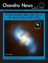
March 2007
Chandra News
Published by the Chandra X-ray Center (CXC) Issue number 14
Chandra and Constellation-X Home in on the Event Horizon,
Black Hole Spin and the Kerr Metric:
The Journey from Astrophysics to Physics
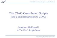
FIGURE 1: Eddington-scaled luminosities of black-hole (red
circles) and neutron-star (blue stars) X-ray transients in quiescence.
The diagonal hatched areas delineate the regions occupied
by the two classes of sources and indicate the dependency
on orbital period.
Astrophysical black holes have the potential
to revolutionize classical black hole physics. After
all, the only black holes we know, or may ever know,
are astrophysical black holes. But how can we make
this journey from astrophysics to physics? In fact, it is
well underway (e.g., see §8 in Remillard & McClintock
2006), and Chandra is making leading contributions
by (1) providing strong evidence for the existence of
the event horizon — the defining property of a black
hole, and by (2) measuring both the spin and mass of
an eclipsing stellar black hole in M33. Meanwhile,
Constellation-X promises to deliver the ultimate prize,
namely, a quantitative test of the Kerr metric. One of
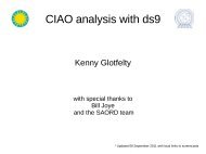
FIGURE 2: (a). ACIS X-ray eclipse light curve of the black
hole binary X-7. The different colors correspond to different
observation epochs. (b). Radial velocity curve of X-7’s O-star
companion.
the most remarkable predictions of black hole physics
is that two numbers specifying mass and spin suffice to
provide a complete and absolutely exact description of
the space-time surrounding a stationary rotating black
hole. Testing this prediction is the most important
contribution that astrophysics can make to black hole
physics.

2 CXC Newsletter
Black Holes are Black: Chandra Points to the
Phantom Horizon
Presently, some 20 X-ray binary black hole candidates
have well-determined masses which exceed the
theoretical maximum mass of a neutron star. This is
taken to be a sign that the objects are black holes. But
do they really have event horizons?
The first test for the presence of the event horizon
was carried out by Narayan, Garcia & McClintock
(1997) using archival X-ray data. However, one had
to wait for Chandra before one could claim definitive
evidence. Figure 1 is a plot of Eddington-scaled Xray
luminosities of neutron-star and black-hole X-ray
binaries in their quiescent or ultralow mass accretion
rate (Ṁ) state. The horizontal axis shows the orbital
period, which according to binary mass transfer models
is a predictor of Ṁ (Menou et al. 1999). The contrast
between the neutron-star and black-hole candidates is
dramatic. At every orbital period, black hole candidates
CONTENTS
Chandra and Constellation-X Home in on the Event
Horizon, Black Hole Spin and the Kerr Metric
1 Useful Chandra Web Addresses 30
Project Scientist’s Report 6 Chandra Data Processing 31
Project Manager’s Report 6 The Chandra Automated Processing System 31
Instruments: ACIS 8 The Chandra X-ray Observatory Calibration Database 33
Instruments: HRC 11 Chandra Data Archive Operations 35
Instruments: HETG 13 CIAO: Chandra’s Data Analysis System 36
Instruments: LETG 16 Status of the Chandra Source Catalog Project 38
Chandra Important Dates 2007 19 Chandra Data Archive 40
Chandra Calibration 20 Absolute Time Calibration for the Chandra X-ray
Observatory
41
Cross-Calibrating Chandra and XMM-Newton 21 The Results of the Cycle 8 Peer Review 43
CXC 2006 Press Releases 23 Chandra-Related Meetings Planned for the Next Year 45
Chandra Fellows for 2007 23 Monte-Carlo Processes ... 47
Running Chandra 24 Chandra Education and Public Outreach 48
Chandra Flight Operations Software Tools Improve
Mission Execution
24 Constellation X-ray Mission Update 51
The Chandra X-Ray Observatory Mission Planning
Process
25 Mission Planning under Bill Forman 52
Chandra, Hardware and Systems 27 HelpDesk 53
Chandra Monitoring and Trends Analysis 27 Chandra Users’ Committee Membership List 53
A Historical Fluence Analysis ... 29 X-ray Grating Spectroscopy Workshop 54
Eight Years of Science with Chandra 30 Mz 3, BD+30˚3639, Hen 3-1475 and NGC 7027 55
X-ray Astronomy School 30 CXC Contact Personnel 55
Chandra Calibration Workshop 30
have Eddington-scaled luminosities that are lower than
neutron stars by two to three orders of magnitude. Even
if we do not scale by the Eddington limit, the difference
is still nearly two orders of magnitude.
The explanation for this result is that accretion in
these quiescent systems occurs via a radiatively inefficient
mode (advection-dominated accretion), as confirmed
through spectral studies. Therefore, the disk
luminosity L disk,

March, 2007
FIGURE 3: Behavior of three key dimensionless quantities (see
text for definitions) that depend only on the black hole spin parameter
a * . The filled circles correspond to nominal estimates of
the spins of (from left to right) LMC X-3, GRO J1655-40, 4U1543-
47 and GRS1915+105 (McClintock et al. 2006). The horizontal
dashed and dotted lines corresponds to a * = 0 and a * = 1, respectively.
In panel a, GM/c 2 = 15 km for M = 10M § .
ence of advection-dominated accretion, there should be
a large luminosity difference between compact objects
with surfaces and those with event horizons. Convincing
confirmation of their prediction is provided by Figure
1, which is an updated version of a similar figure
that appeared first in Garcia et al. (2001; see also Mc-
Clintock et al. 2004). Chandra, which supplied most of
the data shown in this figure, is by far the best telescope
for this work because of its low background.
In addition to the above test, which is based on
luminosity, one could also consider spectral information.
There are strong theoretical reasons to expect the
radiation emitted by the surface of a compact star to be
thermal. Therefore, if the tiny luminosity seen in quiescent
black holes is from the stellar surface, one would
expect the spectrum to be thermal (as it is, for instance,
in most quiescent neutron stars). Observations with
Chandra of the quiescent black hole X-ray binary XTE
J1118+480 show, however, that the radiation comes out
almost entirely in a power-law component, confirming
that this object does not have a surface (McClintock et
al. 2004)
The Spin and Mass of the First Eclipsing Black Hole,
M33 X-7
The Chandra Legacy observations of M33 revealed
the first eclipsing black hole X-ray binary, which
was dubbed X-7 (Figure 2a; Pietsch et al. 2006). At a
distance of 810 kpc, X-7 lies at 100 times the distance
of a typical Galactic X-ray binary. Despite this great
distance, Chandra pinpointed the location of X-7’s Otype
optical counterpart, which has a probable mass of
about 50M § . This massive star’s large velocity amplitude,
K = 110 ± 7 km s -1 (Figure 2b; Orosz et al. 2007),
implies an estimated black hole mass of 10-15 M § .
Once precise values of black hole mass and orbital
inclination have been determined, the 1.4 Msec of
Chandra data will be used further to estimate the spin of
X-7 by fitting its X-ray continuum spectrum to a model
of an accretion disk that includes all relativistic effects.
Recently, the spins of four stellar black holes have been
estimated in this way (McClintock et al. 2006).
As mentioned above, an astrophysical black hole
FIGURE 4: Simulated accretion disk image showing strong non-axisymmetric structure (from simulations of
Armitage & Reynolds 2003).
3

4 CXC Newsletter
FIGURE 5: Simulated Constellation-X observation of iron line variability from the simulation
shown in Fig. 4 assuming a disk inclination of 20 degrees and a black hole with
mass M=3×10 7 M § . The 2-10 keV flux is assumed to be F=5×10 -11 erg s -1 cm -2 , characteristic
of a bright AGN.
is completely defined by just two numbers: its mass and
its dimensionless spin. The latter parameter, called a * ,
is limited to the range 0 (non-spinning hole) to 1 (maximally
spinning hole). A further remarkable prediction
of general relativity (GR) is the existence of a smallest
radius R min for a particle orbiting a black hole. As
shown in Figure 3a, R min depends only on the mass and
spin of the black hole, decreasing from 90 km to 15 km
as the spin increases from 0 to 1 (for M = 10 M § ). The
inner edge of the accretion disk that encircles the black
hole is truncated at this innermost stable circular orbit.
Thus, by fitting the disk spectrum and thereby measuring
the radius of the inner edge of the disk, one can
obtain an estimate of spin. Three dimensionless quantities
of interest are plotted in Figure 3 versus the spin
parameter a * : (a) the radius of the innermost orbit R min ,
(b) the binding energy per unit mass at R min , and (c) the
Keplerian frequency at R min (McClintock et al. 2006).
Also shown in the figure are the nominal values of these
quantities for four black holes.
The black hole mass of M33
X-7 will soon be available (Orosz
et al., in preparation), and it will be
precise because the X-ray eclipse
duration and known distance are
strong constraints, which are not
available for Galactic black hole
binaries. Meanwhile, a preliminary
analysis of all the Chandra
ACIS data shows that it will be
possible to obtain a secure estimate
of spin because the source
was in the required thermal state.
It is a testimony to the power
of Chandra and a wonder to
think that we will soon know the
mass and spin — i.e., a complete
description in GR — of this tiny
and distant black hole.
Do Black Holes Manifest the
Kerr Metric? Testing the Kerr
Metric with Constellation-X
General Relativity makes a
clear and robust prediction: The
space-time structure around an
isolated black hole is described
by the so-called Kerr metric. The
studies discussed above assume the validity of GR and
the Kerr metric in seeking evidence for the event horizon
or estimating black hole spin. Although not discussed
here, spin is also being estimated via studies of
the time-averaged profile of the Fe line (e.g., Brenneman
& Reynolds 2006; Miller et al. 2004), which will be observed
for hundreds of AGN by Constellation-X. The
dynamical tests of the Fe line that we now discuss are
entirely different and aim at providing a quantitative Xray
test of the Kerr metric itself. Constellation-X will
achieve this goal by examining rapid variability of the
broad iron line.
There are two possible origins of iron line variability
that can be used to probe the metric. We expect
the pattern of line emission across the disk to be highly
non-axisymmetric due to non-axisymmetric reconnection/flaring
events in the irradiating corona, as well
as geometric corrugations and/or patchy ionization of
the disk surface itself (see Figure 4). Orbital motion
of the disk combined with the asymmetry in the line

March, 2007
FIGURE 6: 1, 2, and 3-σ confidence contours for the constraints
on spin and radius for a simulated Constellation-X
observation of a single hot spot containing 10% of the total
iron line flux.
emission pattern will induce characteristic variability
of the iron line profile. Figure 5 shows a Constellation-
X simulation of line variability due to orbiting coronal
hotspots, and Figure 6 shows the confidence contours
on black hole spin and hot spot radius that result from
fitting the simulated energy-time track with a library of
theoretical tracks. The superb constraints highlight the
power of iron line variability and suggest the following
experiment for quantitatively testing the Kerr metric.
By fitting many observed tracks with templates that assume
GR, one can determine the mass, spin and radius
for each track. GR then fails if the inferred black hole
spins and masses measured at different radii are not
consistent.
A second kind of iron line variability accessible
to Constellation-X is associated with the light echo of
very rapid X-ray flares across the inner accretion disk.
As well as the “normal” outward-going X-ray echo
(which produces a progressively narrowing iron line),
an inward-moving echo is created by photon propagation
through the curved space-time close to the black
hole. This purely relativistic branch of the echo (which
eventually freezes at the event horizon) produces a
characteristic redward moving bump in the iron line
profile (Reynolds et al. 1999). Comparing observed
reverberation signals with predictions from GR gives
a powerful probe of photon dynamics close to a black
hole and has the potential to falsify the Kerr metric.
References
Armitage, P. J., & Reynolds, C. S. 2003, MNRAS,
341, 1041
Brenneman, L. W., & Reynolds, C. S. 2006, ApJ,
652, 1028
Garcia, M. R., McClintock, J. E., Narayan, R.,
Callanan, P., Barret, D., & Murray, S. S. 2001, ApJ,
553, L47
McClintock, J. E., Narayan, R., & Rybicki, G. B.
2004, ApJ, 615, 402
McClintock, J. E., Shafee, R., Narayan, R., Remillard,
R. A., Davis, S. W., & Li, L.-X. 2006, ApJ, 652,
518
Menou, K., Esin, A. A., Narayan, R., Garcia, M.
R., Lasota, J. P., & McClintock, J. E. 1999, ApJ, 520,
276
Miller, J. M., Fabian, A. C., Reynolds, C. S.,
Nowak, M. A., Homan, J., Freyberg, M.J., Ehle, M.,
Belloni, T., Wijnands, R., van der Klis, M., Charles,
P.A., Lewin, W. H. G. 2004, ApJ, 606, L131
Narayan, R., Garcia, M. R., & McClintock, J. E.
1997, ApJ, 478, L79
Narayan, R., & Yi, I. 1995, ApJ, 452, 710
Orosz, J. A., McClintock, J. E., Bailyn, C. D., Remillard,
R. A., Pietsch, W., & Narayan, R. 2007, ATEL
#977
Pietsch, W., Haberl, F., Sasaki, M., Gaetz, T. J.,
Plucinsky, P. P., Ghavamian, P., Long, K. S., & Pannuti,
T. G. 2006, ApJ, 646, 420
Remillard, R. A., & McClintock, J. E. 2006,
ARAA, 44, 49
Reynolds, C. S., Young, A. J., Begelman, M. C.,
& Fabian, A. C. 1999, ApJ, 514, 164
Jeff McClintock, Ramesh Narayan,
Chris Reynolds, Michael Garcia,
Jerome Orosz, Wolfgang Pietsch
& Manuel Torres
5

6 CXC Newsletter
Project Scientist’s Report
Congratulations to the entire Chandra Team, including
the hundreds of Guest Observers! We’re now
into the eighth year of highly productive Chandra operations.
NASA’s planning now projects Chandra operations
through 2014. We hope and expect that this successful
mission will continue beyond that projection.
Chandra Project Science continues to support activities
addressing radiation damage to and molecular
contamination of the ACIS instrument. Based upon current
trends, neither of these is life limiting; however,
each will progressively impact science performance
throughout the mission. A more serious limitation on
science operations and (perhaps) mission life is the
continuing increase in component temperatures, due
to degradation of Chandra’s thermal blankets. We applaud
the efforts of the mission planning team in dealing
with the increasingly more demanding constraints
due (primarily) to thermal issues.
Within X-ray astronomy, Chandra has pioneered
the definition and allocation of large (LP) and very large
(VLP) projects, which require more observing time than
typical Guest Observer (GO) projects. In this spirit, the
CXC and Project Science this past year sought community
response to the idea of an extremely large project
(ELPs) program, which would allow projects that cannot
be accomplished within the time allocated for a GO,
LP, or VLP. If scientifically justified, one ELP — with
3-5 Ms total exposure — could be selected every 3
years. The proposed ELP program does not impact the
GO program; it would affect the LP and VLP programs
only once every 3 years. Please visit cxc.harvard.edu/
proposer/elp.html for more details.
We invite you to read SPIE paper 6271:07 (2006),
“The role of Project Science in the Chandra X-ray Observatory”.
This is a retrospective look at the Chandra
X-ray Observatory—nee Advanced X-ray Astrophysics
Facility (AXAF)—from the perspective of Project Science.
We presented this paper in the conference Modeling,
Systems Engineering, and Project Management
for Astronomy II, at the SPIE symposium Astronomical
Telescopes 2006. The paper first briefly describes the
Chandra X-ray Observatory, chronicles the Chandra
Program from mission formulation to operations, and
acknowledges the many contributing organizations.
Next the paper discusses the Chandra-AXAF projectscience
function — distributed amongst MSFC, SAO,
and instrument-team scientists — and project-science
activities, especially those performed by MSFC Project
Science. The paper concludes with a summary of some
factors that we believe contribute to the success of a
large scientific project — teamwork amongst all elements
of the project and amongst all project cultures,
a distributed project-science function that encouraged
both cooperation and constructive criticism, and an involvement
of scientists in all aspects of the project. You
may access this and other selected papers by members
of Chandra Project Science at wwwastro.msfc.nasa.
gov/research/papers.html.
In closing, we want to recognize the other present
and past members of Chandra Project Science at
MSFC — Drs. Robert A. Austin, Charles R. Bower,
Roger W. Bussard, Ronald F. Elsner, Marshall K. Joy,
Jeffery J. Kolodziejczak, Brian D. Ramsey, Martin E.
Sulkanen, Douglas A. Swartz, Allyn F. Tennant, Alton
C. Williams, & Galen X. Zirnstein, and Mr. Darell Engelhaupt.
Martin C. Weisskopf, Project Scientist
Stephen L. O’Dell, Deputy Project Scientist
CXC Project Manager’s
Report
Chandra passed its seven year milestone in July
2006 with continued excellent operational and scientific
performance. Telescope time remained in very
high demand, with significant oversubscription in the
Cycle 8 peer review held in June. The observing program
transitioned on schedule in December from Cycle
7 to Cycle 8 and we look forward to the Cycle 9 peer
review in June. The competition for Chandra Fellows
positions was also fierce this year, with a record 104
applicants for the 5 new awards.
The CXC mission planning staff continued to
devote much effort to minimizing the effects of rising
spacecraft temperatures on the scheduled efficiency.
The temperature increase is due in large part to the degradation
of layers of silvarized teflon multilayer insulation
that provide Chandra’s passive thermal control.
During 2005 a number of competing thermal

March, 2007
constraints have resulted in an increased number of
observations having to be split into multiple short duration
segments. This allows the spacecraft to cool at
preferred attitudes but results in a decreased observing
efficiency (down ~4% in the last year) and an increase
in the complexity of data reduction for observers. The
efficiency improved following the relaxation of a thermal
constraint associated with the EPHIN (Electron
Proton Helium Instrument) radiation detector. The
maximum allowed temperature limit was raised from
96˚F to 110˚F in December 2005 following a study that
showed that the instrument can operate safely up to
120˚F. The constraint change provided welcome relief
to the mission planning team. Overall the average observing
efficiency in the last year was 64% compared
with the maximum possible of ~70%.
Operational highlights have included responding
to 9 fast turn-around observing requests that required
the mission planning and flight teams to reschedule and
interrupt the on-board command loads. The year was
a quiet one with respect to interruptions due to high
levels of solar activity, with only 4 stoppages, with 3 of
them in December. Chandra passed through the summer
2006 and winter 2007 eclipse seasons with nominal
power and thermal performance, and handled lunar
eclipses in August and October without incident. Perhaps
most importantly, the mission continued without a
major anomaly or safe mode transition this year.
A number of flight software patches were uplinked.
Two patches were uplinked in July to add onboard
monitoring of selected propulsion line and valve
temperatures. The patches added a new monitor and
replaced 21 of the Liquid Apogee Engine temperature
readings (unused since the ascent phase of the mission)
with 21 -Z side propulsion line and valve temperatures.
Chandra has experienced decreased thermal margins
as the mission has proceeded. The new on-board monitor
mitigates the risk of a frozen propulsion line by ensuring
a transition to normal sun mode in the event that
temperatures fall below a safe trigger threshold.
The on-board gyro scale-factor and alignment
matrix was updated in December. Following the patch
uplink, a series of test maneuvers executed from the
daily load showed that the performance of the pointing
system matched model predictions extremely well.
As anticipated, the number of ‘warm’ pixels in
the Aspect Camera Assembly’s CCD detector has gradually
increased during the mission. Ultimately, this
trend will constrain our flexibility to choose guide stars
7
for spacecraft pointing and aspect reconstruction. To
reduce the number of warm pixels, mission engineers
lowered the ACA’s temperature during the latter part of
2006 to -19˚C, from its previous value of -15˚C. The
number of warm pixels decreased as expected. Because
-19˚C is the lowest temperature at which the ACA can
be controlled, we anticipate the number of pixels to rise
gradually through the remainder of the mission. However,
projections indicate that the effect will not have
an operational impact until well after 15 years of operations.
Both focal plane instruments have continued to
operate well and have experienced no major problems.
ACIS’s Back End Processor rebooted as a result of the
execution of the spacecraft’s radiation safing software
while a bias map was being computed. The event resulted
in a reversion to the launch version of the ACIS
flight software; the current version was uplinked without
impact. ACIS has continued to show an increased
warming trend (along with the overall spacecraft) and
it was decided to ask observers to identify chips that
could be turned off during observations. Each chip
provides approximately 5˚C of additional margin. The
strategy has increased the mission planning team flexibility.
A test was conducted in August of the HRC +Y
shutter select function. During the test, three select/deselect
cycles were run and confirmed full functionality
of the relay. The test verified that after two years
without use, the +Y shutter has not been affected by the
same failure mode as the -Y shutter.
All systems at the Chandra Operations Control
Center continued to perform well in supporting flight
operations. The ground system software content has remained
relatively stable, with an upgrade to improve
mission planning efficiency. A new voice communications
system was installed at the OCC during the fall,
while the OCC’s network infrastructure was upgraded
significantly in January to resolve component end-ofsupport
issues and improve the network’s design and
fault tolerance. The interface with the Deep Space Network
for command up-link and data down-link continued
very smoothly, and the OCC team supported the
transition to new DSN systems, a new Central Data Recorder
at JPL, and a new DSN scheduling system.
Chandra data processing and distribution to observers
continued smoothly, with the average time
from observation to data delivery averaging less than 3
days. The Chandra archive holdings grew by 0.3 TB to

8 CXC Newsletter
4.4 TB (compressed) and now consist of 15.5 million
files.
The third full re-processing of the Chandra archive,
which began in February, is now more than 70%
complete. The re-processed data, which incorporate
the most recent instrument calibrations, are being made
available incrementally through the Chandra data archive.
The reprocessing is expected to be complete
in the summer. Work is progressing on the Chandra
source catalog, with a science review held in February
providing a sound overview of the requirements. An
initial version of the catalog is expected to be released
later this year.
The Science Data System team released software
updates in support of the Cycle 8 observation proposal
submission deadline (March) and Peer Review (June),
and for the Cycle 9 Call for Proposals (December).
Software was released in September to support the
use of optional ACIS chip configurations driven by the
thermal limitations mentioned above.
Sixteen Chandra press releases and 48 image releases
were issued last year. The Education and Public
Outreach team also held a NASA Media Teleconference
in November that announced a new result on
dark matter. The team broke new ground by starting
to release Chandra podcasts through the CXC website.
These have proven very popular by providing a convenient
way to obtain Chandra science highlights and
educational material.
We look forward to the next year of continued
smooth operations and exciting science results, and to
celebrating eight years of the mission at the “8 Years of
Science with Chandra” symposium to be held 22-23
October 2007 in Huntsville, Alabama. We also anticipate
concurrent observations with GLAST following
its launch in November and wish our colleagues well
as they work toward launch.
Roger Brissenden
Instruments: ACIS
ACIS Update for Cycles 8 and 9
[1] Selection of Optional CCDs:
Because of changes in the Chandra thermal environment,
the ACIS Power Supply and Mechanism
Controller (PSMC) has been steadily warming over the
course of the mission. Under current thermal conditions
and assuming an initial PSMC temperature of less
than +30C, observations at pitch angles less than 60 degrees
which are longer than ~50 ks and which consume
maximum power within ACIS (6 CCDs clocking) are
likely to approach or exceed the Yellow High thermal
limit for the PSMC. Figure 7 shows a series of observations
from March 2006. Two ACIS PSMC temperatures
are plotted in green and blue, the pitch angle of
the spacecraft labeled “SAA Angle” is plotted in red,
and the Yellow High limit for these values is plotted
in yellow. The plot shows several observations with
Chandra, as indicated by the times when the pitch angle
is flat and mostly constant. Notice the time when the
pitch angle decreases to 46 degrees, the PSMC temperatures
rise quickly once the spacecraft is in this orientation.
The side A temperature comes very close to the
Yellow High limit. Figure 8 displays the range of pitch
angles for which there are limitations on the time the
spacecraft can spend in that orientation. The range of
pitch angles which are of concern for the ACIS PSMC
is 45-60 degrees.
To counter this, all observers are now being asked
to review their CCD selections and determine which,
if any, of their CCDs can be turned off to prevent the
PSMC from approaching its thermal limits. The RPS
forms and OBSCAT now allow for 6 CCDs with at
least one required (marked as YES) and up to 5 optional
CCDs (marked as OPT1-OPT5). When the observation
is being planned in a short-term schedule, the Flight
mission planning team may turn off one or more of
the optional CCDs starting with OPT1 and proceeding
through OPT2 to OPT5, if necessary, to protect the
PSMC. Please review your CCD selection and determine
which CCDs are not required to achieve your science
goals. Efforts will be made to avoid turning off
optional CCDs unless needed to protect the PSMC.

March, 2007
FIGURE 7: The ACIS PSMC temperatures 1PDEAAT/1PDEABT over a 4 day
period from March 2006. The PSMC temperatures are indicated by the green
and blue data points and the spacecraft pitch angle is indicated by the red line
labeled “SAA Angle”. Note how the PSMC temperatures increase on DOY 86
when the pitch angle is ~46 degrees.
FIGURE 8: Diagram of the range of pitch angles for which the durations of observations
may be limited with Chandra. The affected subsystem is indicated for each range. Pitch
angles of less than 60 degrees are a concern for ACIS.
9

10 CXC Newsletter
FIGURE 9: Composite image of the “bullet cluster”. See text on next page
for discussion.
However, in the interest of scheduling efficiency we
will tend to avoid splitting observations.
If no optional CCDs are selected, six CCDs are
being clocked and the observation MUST be scheduled
at a pitch angle less than 60 degrees, then the observation
is likely to be split into two (or more) observations.
If no optional CCDs are selected, six CCDs are
being clocked and the observation is not constrained
in such a way as to prohibit it, the observation is likely
to be scheduled at a time for which the pitch angle is
greater than 60 degrees. If the observation is assigned
a time in the Long Term Schedule for which the pitch
angle is smaller than 60 degrees, the observation may
be rescheduled for a later date when the pitch angle is
larger based on the detailed scheduling of the time slot
for that observation.
While these restrictions apply to all observations,
those most likely to be affected are those for which the
approved observing time is larger than 25 ks and at least
five required CCDs. Note that even if your observation
is very short, it may occur in a sequence of observations
at bad pitch angles, and it is therefore important
that you consider whether any chips are optional unless
your target is at an ecliptic latitude greater than 60
degrees.
For examples of common selections of optional
CCDs, GOs are encouraged to consult Section 6.1.19
of the Proposers’ Guide.
[2] Updated Energy to PHA Conversion
In cycle 8, a new energy to PHA conversion
will be used for observations with
energy filters. Two sets of conversions will
be used, depending on the aimpoint of the
observation. Observations with ACIS-S at
the aimpoint will use a conversion tailored
for the back-illuminated (BI) CCDs and
those with ACIS-I at the aimpoint will use
front-illuminated (FI) CCD specific conversions.
The BI and FI specific conversions
are more accurate for each type of CCD than
the conversion used in previous AOs. The
assumption is that it is desirable to have the
most accurate gain conversion for the CCD
on which the HRMA aimpoint falls. The
new conversion is ONLY used for creating the command
loads to the instrument which define which PHA
values should be included in the telemetry stream and
which should be rejected. This change does NOT affect
the computation of the energy of an X-ray event
contained in the calibrated events files produced by the
CXC.
The observer should be aware that for observations
which mix CCD type (i.e. BI and FI CCDs on),
the selected conversion (based on aimpoint as above),
will apply to all selected CCDs. This will not affect the
observation if the low energy threshold for the energy
filter (the “Event filter: Lower” parameter) is 0.5 keV
or less as the use of either conversion at these energies
results in essentially no difference in the accepted
events. However, above 0.5 keV, the conversions are
significantly different. Observations which apply an
energy filter with a low energy threshold greater than
0.5 keV will automatically be assigned spatial windows
that allow the FI CCDs to use the FI conversion
and the BI CCDs to use the BI conversion regardless of
aimpoint.
If the reader desires more detail on this, they are
encouraged to consult the following web page:
http://cxc.harvard.edu/acis/memos/acis_gain/web/
compare.html and to send questions to the CXC.
Paul Plucinsky

March, 2007
Figure 9. Three views of the merging cluster of
galaxies 1E0657-56, a.k.a. the “bullet cluster.” Encoded
in pink is an X-ray image from the 500 ks ACIS
exposure, with a prominent “bullet” subcluster visible
at right.
In X-rays, we see the hot intergalactic gas, the
dominant visible matter component in galaxy clusters.
It is overlaid on an optical image, which shows two
concentrations of galaxies belonging to the merging
subclusters.
Galaxies contribute only a small fraction to the
total mass of the cluster, much less than the gas. Encoded
in blue is a map of the total projected mass derived
using the gravitational lensing technique (Clowe et al.
2006, ApJ, 648, L109).
The two peaks of the total mass are clearly offset
from the two peaks of the visible mass (i.e., the hot gas).
This shows that there is something else in the cluster,
much more massive than the most massive visible mass
component. That something else is dark matter.
This observation provided the first direct and unambiguous
proof of its existence, ruling out a competing
possibility that what we thought of as “dark matter”
may in fact be a manifestation of non-Newtonian
gravity on large linear scales (e.g., Milgrom 1983, ApJ,
270, 365). The separation of visible and dark matter,
observed for the first time, is caused by a violent merger,
which we were lucky to observe at exactly the right
time.
Maxim Markevitch
Instruments: HRC
The HRC continues to operate smoothly with no
major problems or anomalies. The ongoing monitoring
of the HRC gain shows a small decrease as a result of
extracted charge, but the need for any increase in the
MCP high voltage to offset the loss of gain is several
years away. In fact, the gain appears to be stabilizing
and it may hold steady for many years or even decades
at the present rate of charge extraction. Continued monitoring
of the HRC X-ray and UV sensitivities shows
no change in instrument performance. The move of the
HRC laboratory from Porter Square, Cambridge, to our
new facility in Cambridge Discovery Park was completed
during the last year. The lab is now up and run-
11
ning and supports on-going HRC flight operations. In
short, it has been a smooth, routine year for HRC as the
flight instrument continues to function well.
A variety of science observations, both GO and
GTO, have been made over the past year with the HRC-
I, the HRC-S in timing mode, and the HRC-S/LETG
combination. We present some science highlights from
the last year, including an HRC-I observation of relativistic
flow in the jets of SS433, and the HRC-S timing of
the pulsar PSR J1357-6429.
An underlying relativistic flow in the jets of
SS433?
In recent years, evidence has come to light for
unseen, highly-relativistic flows in the Galactic neutron
star X-ray binaries Scorpius X-1 (Fomalont et al.,
2000) and Circinus X-1 (Fender et al., 2004). An underlying
flow propagating outwards at high speed energizes
the mildly-relativistic radio-emitting regions
further downstream in the flow, lighting them up via
shock heating. Tentative evidence for this phenomenon
was also seen in simultaneous Chandra and VLA observations
of the powerful, super-Eddington jet source
SS433. ACIS images showed X-ray jets cospatial with
the radio emission, which evolved on timescales of a
few days at angular separations of 10 17 cm from the
center of the system (Migliari et al., 2005). The implied
velocity of the underlying flow was ≥ 0.5c. The
X-ray spectra implied reheating of the jet material to
high (>10 7 K) temperatures by thermalization of the jet
kinetic energy, creating a hybrid plasma dominated by a
population of thermally-emitting particles with a small
(~1%) synchrotron-emitting high-energy tail.
A team led by Drs. S. Migliari and J. Miller-Jones,
and including Drs. R. Fender, M. van der Klis, and J.
Tomsick, proposed for linked Chandra HRC X-ray and
VLA radio observations, in order to simultaneously
study the thermal and non-thermal emitting populations
with the high spatial resolution afforded by the HRC
and the VLA. The rapid readout rate of the HRC would
also prevent pile-up from the X-ray bright core from
hindering the detection of any resolved jets. Four 10ks
observations were made over the course of 8 days,
aiming to track the evolution of the emitting jet knots.
They showed that while the well-known radio jets were
present, tracing out the familiar corkscrew pattern owing
to the precession of the twin beams, no extended Xray
emission was visible. The source was unresolved
with the HRC (see Fig. 10 compared with an earlier

12 CXC Newsletter
ACIS-S observation Fig. 11), suggesting that any underlying
relativistic flow is not persistent, and that the
non-thermal population has a longer lifetime than any
thermally-emitting population. An increase in the Xray
count rate over the course of the four epochs, in line
with the measured radio flux of the core, suggests that
a new phase of activity and jet heating might have been
beginning at this time. Analysis of these data are still
ongoing.
Pulsar J1357-6429
The young and energetic pulsar PSR J1357-6429,
discovered recently at radio frequencies, was the prime
target during two CXO observations performed on
November 18 and 19, 2005 by Drs. Lucien Kuiper and
Mariano Mendez. The HRC-S in imaging mode was
used as focal plane instrument to allow high-precision
imaging and timing. In the combined exposure of 33 ks
for the first time X-rays were detected from PSR J1357-
FIGURE 10: Montage of the four epochs of observation of SS433. Shown in each case is a colormap of the HRC image, with VLA
radio contours superposed. There is no evidence for any extension of the X-ray emission along the radio jets.
FIGURE 11: Colormap of the smoothed Chandra ACIS image of SS433 (2003 July),
with simultaneous VLA radio contours superposed. There is clear evidence for extension
of the X-ray source cospatial with the radio jets. Note the change in scale
between this image and the HRC images, due to the larger PSF of the ACIS instrument.
6429. The spatial distribution of the
events (~170 counts) clearly showed
evidence for the presence of extended
emission (see Figure 12), very likely
an underlying Pulsar Wind Nebula,
along with the point-source emission
from the rapidly spinning (P=166 ms)
neutron star. Accurate spin parameters
from contemporaneous radio observations
made the detection of the pulsed
signal (pulsed fraction 40±12%) at Xray
energies possible (see Figure 13).
This CXO observation demonstrates
that with relatively small exposures
crucial information on the X-ray characteristics
can be derived for weak/
dim, but energetic radio pulsars.

March, 2007
FIGURE 12: HRC-S image of PSR J1357-6429.
FIGURE 13: X-ray light curve of PSR J1357-6429. The period
(166 ms) was determined from radio observations.
Ralph Kraft and Almus Kenter
Instruments: HETG
HETG Status and Calibration
13
The HRMA, HETG, and ACIS continue to perform
superbly together since their memorable debut at
the X-Ray Calibration Facility in Huntsville AL on 18
April 1997. There have been no new HETG-specific
calibration changes in the past year. However small
changes to the ACIS calibration which will show up in
HETGS ARFs are present in the CALDB release 3.3.0,
e.g., the frontside cosmic ray effect of order 2-to-4%
and an improved Si-edge calibration. Attention is turning
to cross-calibration of the Chandra instruments
with other X-ray missions and instruments as described
in the article by Herman Marshall in this issue.
High-Resolution Spectroscopy Workshop
A spectrum by any other wavelength would be as
“Sweet!”
The Chandra X-ray Center is hosting a workshop
11-13 July 2007 entitled “X-Ray Grating Spectroscopy”
[1]; one of the sub-themes is spectroscopic studies
in conjunction with other wavebands. Across all
wavebands high-resolution spectroscopy is sensitive
to the geometry and kinematics of the source through
Doppler and absorption effects. Likewise, the plasma
state can be probed through line strengths and ratios
from a variety of ions. For example, FUSE can measure
O VI while current X-ray spectrometers include
lines of O VII and O VIII ions. X-ray measurements
of high-ionization states of Si in the SNR Cas A [2]
can be compared with low-ionization Si seen with the
Spitzer IRS [3] to study both shocked and “unshocked”
SN material. As a final example, SN 1987A has been
studied with HST-STIS [4], the Chandra HETG [5] and
LETG [6], and with ground-based spectrometers that
provide very high resolution ( E/dE ~ 5×10 4 ) over a
full 2D field, e.g., the ESO/VLT-UVES [7,8]. Note that
although optical wavelengths are involved, ionization
states as high as Fe XIV can be measured and have relevance
to the X-ray measurements, Figure 14. (This year
further HETG and LETG observations of SN 1987A
are planned.)

14 CXC Newsletter
Normalized flux
4
3
2
1
[Fe X] λ6375
[Fe XI] λ7892
[Fe XIV] λ5303
0
5000 5500 6000 6500 7000
Days after explosion
FIGURE 14: Ground-based measurements of “coronal” lines from SN 1987A.
The growth over time of the optical Fe XIV flux (left, circles) shows a trend similar
to that of the low-energy X-ray flux (right) which includes emission from Fe XVII
lines (as shown in Kjaer et al. [7], from the detailed work by Gröningsson et al.
[8].)
Not surprisingly, there is also a commonality
across wavebands in the analysis and modeling challenges
and techniques for high-resolution observations.
These generally include 3D geometry and photon propagation
modeling. The HETG group is involved in this
domain through the Hydra project; for a sampling of
the range of activity in this growing area see the list of
related work by others on the Hydra web pages [9].
HETG Science: The Joy of Phase
We don’t usually get to view an astronomical
source from other than a single direction but some
systems, such as binaries, rotate on human timescales.
Observing these systems at different orientations, orbital
phases, helps us in getting a full 3D picture of the
system. The following text and figures give a brief hint
of some recent work which demonstrates the potential
of multi-phase observations when combined with highresolution
spectroscopy.
4
3
2
1
X−ray (0.5−2 keV)
0
5000 5500 6000 6500 7000
The massive stars in the system
WR 140 are in a 7.94 year eccentric
binary orbit and their stellar winds are
in continuous collision. Work by Pollock
et al. [10] shows clear changes in
the amount of absorption with orbital
phase, Figure 15. In addition, changes
in the line profile of the Si XIV lines
agree with the relative direction of the
moving wind material at the different
phases. Although the wind shock is
ongoing and stationary, the shocked
material is not in ionization equilib-
rium (instead, well fit with a vpshock
model) and possibly includes nonthermal particle acceleration
— basic physics similar to shocks in supernova
remnants.
Eta Car consists of a 120 solar mass primary that
is in “a phase of immense mass ejection” and in orbit
with a companion in a 5.54 year binary period. Behar
et al. [11] have taken a high-resolution look at archival
HETG data on Eta Car, concentrating on the evolution
of Si and S line shape versus phase near periastron (the
binary components’ closest approach), Figure 16. At
this phase they see enhanced high-velocity gas which
they intriguingly suggest may be a “hot jet, or collimated
fast wind”. Stay tuned for more data from the
next periastron in January of 2009.
The Vela X-1 system consists of a neutron star
(pulsar) orbiting a massive B supergiant companion
with a period of 8.964 days. The companion’s wind
is accreted onto the neutron star giving a bright X-ray
emission which illuminates and photoionizes the stellar
wind. The recent work by Watanabe et al. [12] com-
Figure 15: Emission from the
colliding winds in WR 140.
At left, HEG and MEG spectra
are shown before (dotted)
and after (solid) periastron.
The change in viewing direction
between these observations
is indicated in the diagram
at right. (From Pollock
et al. [10].)

March, 2007
FIGURE 16: (left) Mean
line profiles from the Eta
Car system as seen with
HETG observations. An
outflow with velocities up
to -2000 km/s dominates
the line profile as the system
approaches periastron
(point-up triangles.)
(From Behar et al. [11].)
(right) Line profiles of the
Eta Car system as seen
with HETG observations.
In the upper panel, the Si
XIV line profile at phase -0.028 is well resolved by - and consistent between - the
HEG and MEG spectra. In the lower panel, comparison of the line profile at different
phases shows that velocities up to -2000~km/s appear in the line profile (phase
-0.028) as the system nears periastron. (From Behar et al. [11].)
bines detailed photoionization calculations with Monte-Carlo
simulations of photon propagation to model
the observed spectra at different orbital phases, Figure
17. Their results nicely confirm and give parameters
for an ionized stellar wind and a cold cloud of material
behind the neutron star. However, the model and data
do not agree in the detailed line shapes, indicating that
in places the wind speed is lower than expected. They
show that this difference could be due to a reduced
population of UV-absorbing ions in the wind caused by
photoionization as the wind nears the neutron star. So,
the next step is a “fully self-consistent 3D model including
the X-ray photoionization”...
“Laissez les bons spectra rouler!”
Dan Dewey, for the HETG Team
15
References
[1] Workshop web page: http://cxc.harvard.edu/
xgratings07
[2] Lazendic, J.S., et. al. 2006, ApJ 651, 250.
[3] DeLaney, T., et al. 2007 to appear.
[4] Pun, C.S.J., et al. 2002, ApJ 572, 906.
[5] Michael, E. et al. 2002, ApJ 574, 166.
[6] Zehkov, S.A., et al. 2005, ApJ 628, 127 and
2006, ApJ 645, 293.
[7] Kjaer, K., et al. 2006, astro-ph/0612177 .
[8] Groningsson, P., et. al. 2006, A&A 456, 581.
[9] Hydra-related papers: http://space.mit.edu/hydra/related.html
[10] Pollock, A.M.T., et al. 2005, ApJ 629, 482.
[11] Behar, E., et al. 2006, astro-ph/0606251 .
[12] Watanabe, S., et al. 2006 ApJ 651, 421.
FIGURE 17: HETG observations of Vela X-1. At left HEG spectra at three phases are compared with simulated spectra from a detailed
model of the photoionized stellar wind; this initial model does well, except at the Fe-K line in phases 0.25 and 0.5. This extra Fe-K
emission is accounted for in the system (diagram at right) by reflection from the companion’s surface and photoionized emission from
a small, cold cloud behind the neutron star, possibly an “accretion wake” (from Watanabe et al. [12]).

March, 2007
FIGURE 18: The first high resolution X-ray spectrum of a planetary
nebula. BD+30˚3639 was observed by LETG+ACIS-S
in February and March of 2006. Note the relatively strong
lines of C and the very weak Fe XVII resonance line at 15Å
that are signatures of shell helium burning and the s-process
on the AGB (from Kastner et al. 2006).
emitting shock and the extended emission first seen by
Kastner’s group using ACIS.
The ACIS spectrum hinted at enrichment of the
hot gas with nuclear burning products. Despite the object
lying at perennially bad pitch for Chandra, Kastner
and collaborators obtained the first grating spectrum of
the PN in February and March of 2006. The LETG revealed
clear signatures of modified abundances: C/O
about 20 times the solar value with N/O less than solar,
implying a C/N enhancement by a factor > 20; Ne/O ~
4 times solar, but Fe/O only 1/10th solar-see the spectrum
in Figure 18. The X-ray emission emanates from
a layer originally deep within the stellar envelope, and
the large C overabundance can be traced to the Heburning
shell of the progenitor AGB star. Kastner and
colleagues attribute the Ne enhancement to α-capture
reactions on the nitrogen chain 14 N(α, γ) 18 F(β + ) 18 O(α,
γ) 22 Ne, with 22 Ne(α, n) 25 Mg supplying neutrons for
the s-process, probably along with 13 C(α, n) 16 O; Fe
seed nuclei are then depleted by neutron capture to
form heavier elements such as the smoking gun, Tc,
first found by Merrill.
The observed plasma temperature and spatial
characteristics can also be combined with pre-PN AGB
models to begin to understand better the specifics of
the envelope ejection itself. It is already clear that the
X-ray temperature of 2.5×10 6 K is too cool based on the
currently observed wind speed of ~ 700km s -1 , possibly
hinting at a slower wind in the recent past.
All in all, not bad for a star all dredged-up with
nowhere to go.
17
RS Ophiuchus Explodes: The Brightest Supersoft
X-ray Source
It takes about a thousand years to form a planetary
nebula, and envelopes are ejected at very modest speeds
of tens of km s -1 . If you want to watch things move a
bit faster, nova explosions offer the “Stellar Evolution
While You Wait” experience.
The symbiotic recurrent nova RS Ophiuchi (HD
162214) was found to be visible to the unaided eye on
2006 February 12 by Japanese amateur astronomers
(Narumi et al 2006). It has previously undergone five
known outbursts, in 1898, 1933, 1958, 1967, and 1985.
RS Oph is the eponymous member of its subclass of
binaries thought to comprise a white dwarf accreting
from the wind of a red giant companion that does not
fill its Roche lobe. About every 20 years, enough material
from the red giant builds up on the surface of the
white dwarf to produce a thermonuclear runaway. In
less than a day, the otherwise quite dim white dwarf
brightens to more than 100,000L § .
This outburst was followed at different phases by
several space-based facilities, including RXTE, Swift,
HST, Spitzer, XMM-Newton and Chandra. Under the
guidance of Julian Osborne (Leicester University) Swift
has followed the X-ray evolution of the object from day
3.2 onwards; the lightcurve is shown in Figure 19. The
X-ray flux declined steadily from day 4 onwards until
day 29, when it was seen to rise strongly whilst undergoing
wild variations. This was followed by a period of
relative stability and then a slow decline.
The initial bright X-ray emission from RS Oph
in the first few days of the outburst is thought to be
caused by shock-heating of the ambient plasma of the
extended wind of the red giant by the blast wave from
the thermonuclear explosion. RS Oph presents one of
the best examples of a momentum-conserving shock in
an astrophysical source that evolves in a human lifetime.
“In terms of stellar evolution,” as Mike Bode
(Liverpool John Moores University) put it, “our current
observations are enabling us to explore an analogue to
a supernova remnant, but evolving over months, rather
than millennia”.
RS Oph was first observed by the Chandra HETG
at the end of the 13th day as a Directors Discretionary
Time target of opportunity lead by Sumner Starrfield
(Arizona State University). At that time, the bulk plasma
velocities of the expanding blast wave were of order

18 CXC Newsletter
FIGURE 19: The impressive Swift XRT light curve of RS Oph from Osborne
et al. (2006), with insets showing the times at which the LETGS and XMM-
Newton RGS obtained high resolution spectra (Ness et al. 2007).
1700 km s -1 . The sharp rise in X-ray flux
on day 29 ushered in the brightest Supersoft
Source (SSS) phase that has ever
been observed (Osborne et al. 2007): by
then the envelope had thinned sufficiently
to view the central star. The strong
variability remains unexplained at present,
but is possibly associated with either
nuclear burning instability or absorption
by patchy but thick condensations.
As shown in Figure 19, subsequent
to the initial HETG observation of the
blast wave Chandra LETG caught the
SSS phase twice, and the first of these
got a nibble of the strong variability at
SSS onset. The LETG analysis, lead by
Chandra Fellow Jan-Uwe Ness (Arizona
State), shows a remarkable spectrum
in which emission lines shortward of 15
Å due to H-like and He-like ions of Mg
and Ne from the blast wave plasma are
seen simultaneously with the hot
(~ 680,000 K) absorbed, thermal SSS. Figure 20 illustrates
spectra from the first observation during which
RS Oph was entering its SSS phase while exhibiting
violent variations in soft X-ray flux. Shown are spectra
from relatively low and high flux states seen during
the observation. The jagged coastline of the soft thermal
component is not noise: close inspection shows
the bumps and wiggles to correspond to absorption by
abundant species, including O and N in He-like and
H-like forms, and the neutral O edge and prominent
1s-2p resonance. This absorption has sculpted emission
FIGURE 20: Comparison of LETGS spectra extracted from high-flux and
low-flux intervals in ObsID 7296. The high and low states cannot be explained
by a uniform variable absorption, and must instead be caused either
by thick clumps with varying line-of-sight coverage, or by changes in the
source luminosity such as through nuclear burning instability (from Ness et
al. 2007).
lines sitting on the continuum into the
P Cygni-like profiles shown in Figure
21; the absorption troughs formed in
the expanding atmosphere are located
~1300 km s -1 from the rest frame. In
the later observation, these absorption
troughs are seen to have slowed to 800
km s -1 .
One thorny issue with SNe Ia
that currently form the basis for that
minor backwater of modern astrophysics-the
existence of dark energy−is
that we don’t really know which binary
objects they come from. RS Oph
is a possible SNe Ia progenitor. The
key issue is whether or not it is able
to make a net gain of material with time, or whether its
mass declines after each outburst event as a result of the
explosion. The Chandra spectra of both the blast wave
and SSS phases should in time help provide estimates
of the accreted and ejected mass, and probe the site of
thermonuclear runaway using the characteristics and
chemical composition of the puffed-up atmosphere of
the hot SSS.
LETG Programmatics
The LETG itself continues to perform flawlessly.
Detectors are not so well-behaved. During the last few

March, 2007
years, we have noticed that the HZ43 LETG+HRC-S
data show a steady drop in the QE, amounting to a ~5%
decline at wavelengths longer than 50Å since launch.
Superimposed on the monotonic drop are 1-2% fluctuations
that are statistically significant. These effects
are currently not well-understood and investigation is
ongoing.
Recent activities of the instrument team also includes
an updated HRC-S QE file with corrections near
the O-K edge that should appear in the next CALDB
release. This addresses problems that arose from the
in-flight calibration using the primitive oversimplified
edge structure of the ISM absorption previously avail-
FIGURE 21: P Cygni profiles of O VII, O VIII and N VII lines
seen during the SSS phase of the RS Oph 2006 outburst. The
absorption troughs are superimposed on emission lines and
are blue-shifted by 1300 km s -1 (from Ness et al. 2007).
19
able. The new QE was based on new R-Matrix computations
of neutral and ionized ISM absorption structure
published recently by Garcia et al (2005).
Future work will include revisions of the low-energy
(< 0.25 keV, > 50Å) HRC-S QE, a set of HRC-S
gain correction files (one for each year) to account for
secular gain trends observed, and further updates to the
HRC-S degap correction coefficients table to improve
empirical wavelength corrections from both line and
continuum sources.
Bibliography
Kastner, J. H., Sam Yu, Y., Houck, J., Behar, E.,
Nordon, R., & Soker, N. 2006, IAU Symposium, 234,
169
Kastner, J. H., Soker, N., Vrtilek, S. D., & Dgani,
R. 2000, ApJL, 545, L57
García, J., Mendoza, C., Bautista, M. A., Gorczyca,
T. W., Kallman, T. R., & Palmeri, P. 2005, ApJs,
158, 68
Merrill, P., 1952, Science, 115, 484
Narumi, H., Hirosawa, K., Kanai, K., Renz, W.,
Pereira, A., Nakano, S., Nakamura, Y., & Pojmanski, G.
2006, IAUCirc, 8671, 2
Ness, J-U., et al, 2007, ApJ, submitted
Osborne, J., et al, 2007, Science, submitted
Schmitt, J. H. M. M., & Ness, J.-U. 2002, A&Ap,
388, L13
Jeremy Drake
Chandra Important Dates 2007
Cycle 9 Proposals due March 15, 2007
Users’ Committee Meeting April 25-26, 2007
Cycle 9 Peer Review June 19-22, 2007
X-ray Grating Spectroscopy Workshop July 11-13, 2007
Cycle 9 Budgets Due September 13, 2007
Eight-Year Chandra Science Symposium October 23-25, 2007
Cycle 9 EPO Electronic Deadline October 19, 2007
Cycle 9 EPO Hardcopy Deadline October 26, 2007
Chandra Fellows Symposium October, 2007
Users’ Committee Meeting October, 2007
Chandra Fellowship Applications Due November, 2007
Cycle 9 EPO Review November, 2007
Cycle 9 Observations Start December, 2007
Cycle 10 Call for Proposals December, 2007

20 CXC Newsletter
Chandra Calibration
ACIS
Most of the ACIS calibration efforts during the
past year centered on developing cti-corrected (both
parallel and serial) products for the BI chips S1 and S3
at a focal plane temperature of T=-120˚C. This was a
large undertaking and required the development of new
software, a restructuring of the calibration database
as well as new calibration products. The cti-corrected
products for the BI chips were released in CALDB 3.3
on Dec. 18, 2006 and included: new trap maps, QE uniformity
maps appropriate for cti-corrected data, timedependent
gain corrections, and a matrix used to compute
the spectral response at a given location on a given
chip. With this version of the CALDB, all 10 chips
on ACIS now have cti-corrected calibration products.
The cti-uncorrected products are still required to analyze
data taken in graded mode, which cannot be cticorrected.
The response of the BI chips is very uniform
after applying the cti-corrections. These products
were extensively tested with data from the ACIS external
calibration source as well as several astronomical
sources, in particular, the oxygen rich supernova
remnant E0102-72. The 1σ uncertainty in the gain is
0.3% for cti-corrected data and is nearly independent
of energy and location on the chips. This was actually
the requirement imposed on the development of the cticorrected
products for both the BI and FI chips. Thus,
all ACIS chips now have comparable gain uncertainties.
The 1σ uncertainty in the FWHM of a spectral
line after applying the cti-corrections is approximately
20 eV for the BI chips and is also nearly independent of
energy and location on the chips.
Also released in CALDB 3.3 was a correction in
the ACIS QE near the Si-K edge. Gratings data showed
that there was a 4% residual over a 20eV energy band
near the Si-K edge using the previous version of the
ACIS QE. This residual was due to a simplifying assumption
in the treatment of Si K-α escape peak in the
ACIS model. The new ACIS QE applies to both BI and
FI chips.
There now exists a complete, homogeneous, set
of ACIS calibration products for TE data taken in faint
or very faint mode at a focal plane temperature of -120
C, which comprises the bulk of ACIS observations tak-
en since launch. The primary ACIS calibration efforts
at the present time are to improve CC mode calibration,
graded mode calibration, and the calibration of data
taken at a focal plane temperature of -110˚C (data taken
during the first 3 months after launch).
HRC
To further improve image reconstruction of HRC-
I data, we performed a raster scan of Capella (twenty 5
ksec observations) on the inner portion of the detector in
AO7. A complementary raster scan on the outer portion
of the HRC-I will be carried-out in AO8. The observations
acquired in AO7 were used to refine the HRC-I
de-gap map which was released in CALDB 3.2.3 on
Aug. 9, 2006. Reprocessing HRC-I data with the new
de-gap map sharpens the PSF by about 5% relative to
data processed with the earlier version of the HRC-I
de-gap map. For example, reprocessing a long on-axis
observation of AR Lac with the new HRC-I de-gap map
produces 50% and 90% encircled energy radii of 0.41”
and 0.93”, respectively.
Prior to the release of CALDB 3.3, both the HRC-
I and HRC-S only had a single time-independent gain
correction file. A set of time-dependent gain correction
files (one for each year since launch) was released
for the HRC-I in CALDB 3.3. These new products can
be used to generate consistent energy-invariant HRC-I
hardness ratio images. Work is in progress to develop
a set of time-dependent gain correction tables for the
HRC-S. While detailed spectral analysis cannot be carried-out
with HRC-I or HRC-S data, these detectors are
capable of distinguishing between hard and soft sources
(see Ch.7 of the POG). We have also released rmfs for
both the HRC-I and HRC-S which can help with the
interpretation of the hardness ratio images.
HRMA
The optics team has been actively engaged in
porting the entire SAOsac raytrace software package
to Linux. The initial motivation for this project was
to produce a portable version of the raytrace code that
could be used by Chandra observers to facilitate their
data analysis. A preliminary version of this software
was delivered to Data Systems in Jan., 2007 for testing
and integration into Level III processing. Verification
of this software is in progress.
Larry David for the Calibration Team

March, 2007
Cross-Calibrating Chandra
and XMM-Newton
Overview
There has been an ongoing effort to compare
results from Chandra and XMM-Newton and other
X-ray astronomy missions. Results are available on a
new dedicated web page, http://space.mit.edu/ASC/calib/crosscal/
and were presented to the Chandra User’s
Committee (see http://cxc.harvard.edu/cdo/cuc/cucfile06/oct06/Marshall_CUC_Oct06.pdf).
Here, I summarize
this work and some of the major results, uncertainties,
and plans.
Due to the different angular resolutions of the
telescopes involved, most cross-calibration observations
have involved point sources. In order to avoid
pileup and to check more components of the system,
the transmission gratings on Chandra are inserted for
most simultaneous observations. Because there are two
grating assemblies that can be used and two detectors,
the common combinations are usually implemented sequentially
during cross-calibration campaigns. In other
telescopes such as XMM, several instruments are used
at the same time. Due to observing constraints that vary
by observatory, cross-calibration campaigns are rare,
usually performed once or twice per year. Observations
of extended sources are also used in calibration, taking
advantage of their unchanging fluxes and occasionally
line-rich spectra.
Comparing Chandra and XMM-Newton Spectra
These results are summarized on web pages
maintained by both the Chandra and XMM-Newton
projects. See http://space.mit.edu/ASC/calib/crosscal/
for the CXC web page and http://xmm.esac.esa.int/external/xmm_sw_cal/calib/cross_cal/index.php
for the
page developed by XMM-Newton ESAC scientists.
See also the XMM-Newton technical document CAL-
TN-0052 (available on-line at http://xmm.esac.esa.int/
docs/documents/CAL-TN-0052-3-0.ps.gz).
There have been 10 successful cross-calibration
campaigns to observe extragalactic targets with nearly
featureless spectra using both XMM-Newton and
Chandra. Three targets have been used: 3C 273, PKS
21
FIGURE 22: Shows three examples from figure 3 of the CXC
cross-cal web page. The fluxes for the Chandra data were
computed in energy bins 5% wide.
2155-304, and 1H1426+428. The Chandra configurations
include the HETGS, the LETG with ACIS-S,
and the LETG with HRC-S. Results are available at
the aforementioned web sites for several of these campaigns.
The two projects have taken somewhat different
approaches to comparing data. The ESAC web
pages show joint spectral fits using XSPEC and give
the spectral parameters derived. For example, fitting a
broken power law model to the June 2005 observations
of 1H126+428, the 1 keV normalization is 0.01493(6)
(in ph/cm 2 /s/keV) for the joint fit of all data, while the
normalization is 0.0140(4) medium energy grating
(MEG) portion of the HETGS. Fits to the XMM PN
data alone gave a normalization of 0.01525(8). While
these normalizations are formally inconsistent at the
3σ level, the difference is under 10% and the HETGS
high energy grating (HEG) normalization, 0.0148(6), is
within 1σ of that of the PN. Comparing spectral indices

22 CXC Newsletter
gives a similar result: the high energy photon index (E
> 1 keV) is 2.160(8) for the PN and 2.006(47) for the
HEG. These are formally inconsistent while the low
energy indices are almost identical: PN gives 1.893(7)
and the MEG gives 1.892(53). All parameters from the
fits to the August 2005 LETG/ACIS-S observation of
PKS 2155-304 were within 1-2σ of the corresponding
values from the PN fits and for the LETG/HRC-S observations
of the same target and month, only the high
energy photon index was discrepant at more than 3σ.
More comparisons are being prepared.
On the CXC web page, the fits to the PN are
compared directly to Chandra spectra in order to show
more detail. Figure 22 shows three examples from figure
3 of the CXC cross-cal web page. The fluxes for
the Chandra data were computed in energy bins 5%
wide. These comparisons indicate that the XMM and
Chandra spectra agree generally to better than 10%
over a wide energy range. Some systematic differences
are still apparent that aren’t quite consistent between
observations. These differences are still under investigation.
Comparisons of spectral fits to XMM-Newton PN
data to coarsely binned Chandra grating spectra
The fluxes for the Chandra data were computed
in energy bins 5% wide. These comparisons indicate
that the XMM and Chandra spectra agree generally to
better than 10% over a wide energy range. Uncertainties
in the XMM spectral fits aren’t shown but there
may still be some systematic differences that aren’t
fully consistent between targets. These differences are
still under investigation.
Comparing Fluxes in Specified Bandpasses
Another approach being used to compare XMM
and Chandra results is to estimate fluxes in fixed bandpasses.
This method gives a somewhat straightforward
way of comparing XMM instruments and has now been
applied to two of the simultaneous Chandra/XMM observations.
For the December 2001 observation of PKS
2155-304, the LETG/ACIS fluxes in the 0.85-1.50,
1.50-4.00, and 4.0-10.0 keV bandpasses were consistent
within 5% of the fluxes computed from model fits
to PN data. The LETGS-derived flux in the 0.54-0.85
keV band was almost 10% lower than the PN value,
which appears to be consistent with fluxes determined
from the XMM MOS detectors. Comparisons using
the HETGS data from the June 2005 observation
of 1H1426+428 give similar results: MEG and MOS
fluxes are 7-13% lower than PN fluxes in the lowest
band, within 3% in the 0.85-1.50 keV band, and 5-12%
higher in the 1.5-4.0 keV band. In the highest energy
band, the MOS is high by about 15% but the HEG flux
is slightly lower but consistent with the PN flux. This
work is continuing with the remaining targets from the
cross-cal campaigns.
Cross-Calibration of Chandra and Suzaku
In May, 2006, PKS 2155-304 was observed by
Suzaku, Chandra, and XMM-Newton.
Preliminary results from joint Suzaku-Chandra
fits were presented by M. Ishida at the June 2006 international
calibration meeting in Reykjavik, Iceland. The
meeting was the first one for a newly formed group,
called the International Astronomical Consortium for
High Energy Calibration (IACHEC, see http://www.
iachec.org/). Ishida showed that pure power law fits to
the Suzaku XIS spectra gave normalizations consistent
with the LETGS value to within 4% and that the photon
indices agreed within uncertainties.
Summary
While the existing effective areas appear to be
good to better than 10% over most of the Chandra energy
range, we continue to work on ways to determine
what systematic errors remain and to work jointly with
other projects to improve the agreement among all Xray
observatories.
Herman L. Marshall

March, 2007
Table 1 - Chandra 2006 press releases.
Date PI Objects Title
01-10-2006 Thomas Statler
56 elliptical
galaxies
23
NASA’s Chandra Finds Black Holes Stirring Up Galaxies
02-03-2006 Kristian Pedersen NGC 5746 Detection of Hot Halo Gets Theory Out of Hot Water
03-23-2006 Alan Stockton
04-24-2006 Steve Allen
4C37.43 and
3C249.1
9 elliptical
galaxies
NASA’s Chandra Finds Evidence for Quasar Ignition
NASA’s Chandra Finds Black Holes Are ‘Green’
06-01-2006 Bryan Gaensler IC 443 The Case of a Neutron Star with a Wayward Wake
06-21-2006 Jon Miller GRO J1655-40 Black Hole Paradox Solved by NASA’s Chandra
08-08-2006 Max Bonamente
38 galaxy
clusters
Chandra Independently Determines Hubble Constant
08-18-2006 Doug Clowe 1E 0657-56 NASA Finds Direct Proof of Dark Matter
09-18-2006 Jacco Vink RCW 86
CXC 2006 Science Press Releases
See http://chandra.harvard.edu/press/press_release.html for more details.
New Evidence Links Stellar Remains to
Oldest Supernova Remnant
10-05-2006 Bill Forman M87 Chandra Reviews Black Hole Musical: Epic but Off-Key
11-15-2006 Michael Stage Cas A Chandra Discovers Relativistic Pinball Machine
Chandra Fellows for 2007
Megan Watzke
This year we had a record number of applications for Chandra Postdoctoral Fellowships. The list of
Chandra Fellows for 2007 has just been finalized and is provided below. Keep an eye on our web pages
for information about the Chandra Fellows Symposium (October 10, 2007) and the annual Fellowship
competition (November 2007).
PhD Institution Host Institution
John Fregeau MIT Northwestern (yr1)
KITP-USCB (yrs 2&3)
Jonathan McKinney U. Illinois
Ian Parrish Princeton Berkeley
Jesper Rasmussen U. Copenhagen Carnegie Obs.
Jerremy Schnittman MIT Johns Hopkins
Nancy Remage Evans

24 CXC Newsletter
Running Chandra
There were a number of discussions about Chandra, particularly behind the scenes operations presented at the
SPIE Conference 6270, “Observatory Operations: Strategies, Processes, and Systems”. Summaries of these discussions
are presented here, but the full discussion can be found in Proc. SPIE v 6270 (2006).
Editor
Chandra Flight
Operations Software Tools
Improve Mission Execution
A full discussion of this topic is given in the
SPIE Proc 6270, 2006
FIGURE 23: The Chandra Mission Planning process.
Over the first 6 years of the Chandra mission,
the Flight Operations Team (FOT) has developed several
ground software applications intended to help improve
the efficiency of operating the Observatory. In
May of 2006, a paper was presented at the SPIE As-
tronomical Telescopes and Instrumentation Conference
in Orlando Florida highlighting these tools and way in
which they’ve benefited the FOT. Several of these tools
utilize commercial off the shelf software products such
as Matlab, while others are completely home grown.
The tools are introduced here but more fully discussed
in the SPIE paper.
The FOT Mission Planning process (Figure 23)
starts with the receipt of a weekly Observation Request
(OR) list from the Science Mission Planning Team.
This unordered OR list contains all of the information
needed to schedule the individual observations during
the planning week. After receipt of the OR list, the
FOT Mission Planners add Engineering Requests and
then start the process of ordering the observations into
the most efficient possible schedule while at the same
time ensuring that spacecraft and mission constraints
are not violated.
This is a complicated process which has changed
considerably since the beginning of the mission. The
FOT has developed a set of software tools based on
the Matlab scripting language to assist in this process.
The ORViewer is utilized to assist the Mission Planners
in optimally ordering observations. It is a graphical
tool which shows the user different views of the observations
and maneuver paths between observations.
It works in conjunction with two other MP tools, the
Maneuver Constraint Checker (MCC) and the SAU-
SAGE (the Simple AXAF User Selected Acquisition
and Guide star Editor).
The MCC is another graphical tool which shows
the Mission Planners all constraints which might affect
the way in which the weekly schedule can be assembled.
Some of these constraints include inertial
constraints such as lunar, solar, and earth constraints.
Others are temperature related and have to do with protecting
spacecraft units. The MCC also allows users to
view the predicted spacecraft momentum state, antenna
views, and other important planning parameters.

March, 2007
Other FOT tools are used to support other aspects
of operations such as real-time telemetry monitoring.
One of the primary tools used by the FOT in telemetry
monitoring is called GRETA. GRETA displays telemetry
data in both a tabular layout and also in plots. Users
may select any telemetry point to display. GRETA displays
are used daily in operations to monitor the health
and safety of all of the observatory systems. In addition
to the display capabilities in GRETA, GRETA also
monitors certain telemetry points to ensure that they do
not exceed pre-specified limits. This limit monitoring
process is the front line of Observatory protection. Any
limit violation is immediately noticed and reported by
the on-console operators to the engineering team for
immediate response and analysis.
The final set of FOT tools which are utilized in
nominal operations of the vehicle are web based tools
such as the OCCWeb and the Integrated Flight Operations
Timeline (IFOT). These tools are used to give
users information to critical operations data. The OC-
CWeb is used to help individuals on the various operations
team to find data about operations including
how the spacecraft works, minutes from key meetings,
ground stations status, etc. In addition, the OCCWeb
provides an up to the minute snapshot of the mission including
information such as current instrument in use,
target name, altitude, and news and alerts. IFOT allows
users to enter and query past mission events such as
times of safing events, Deep Space Network communication
passes, observations, etc. These tools are used
by operations personnel to better conduct their day-today
tasks.
FOT tools have been developed over a long time
span and have been used to enhance operational efficiency
and effectiveness. There are five primary reasons
for the development of such tools. They are as
follows.
* Changing Requirements
* Lack of visibility into complex processes
* Need for more organized data management
* Inefficiency in current processes
* Reduction of errors
The FOT tools have helped in all of the areas to
make the Chandra mission as successful as possible.
Dan Shropshire, Sabina Bucher, and Joe Rose
25
The Chandra X-Ray
Observatory Mission
Planning Process:
Managing and Implementing
Constraints
ABSTRACT
Planning an observation schedule for groundbased
and space-based telescopes alike requires careful
constraint management and implementation. Scientific
constraints, which meet an observer’s desire to
maximize science returns, must be weighed against the
physical constraints and capabilities of the telescope.
Since its launch in 1999, the Chandra X-Ray Observatory
(CXO) has provided excellent science in spite
of evolving constraints, including the proliferation of
constraint types and varying degrees of restriction. The
CXO observation schedule is generated on a weekly
basis, yet the mission planning process maintains the
flexibility to turn around a target-of-opportunity (TOO)
request within 24-hours. This flexibility is only possible
when all personnel responsible for schedule generation-flight
operations engineers, science operations
personnel, and program office support - are actively involved
in constraint management. A proper balance of
software tools, guideline documentation, and adequate
subjective judgment is required for proper constraint
implementation. The decision-making process employed
by mission planning personnel requires accurate,
complete, and current constraint information.
This retrospective examines the existing constraint
management process from a mission planning
perspective. Topics include: introduction of constraints
to the mission planning pipeline, the adaptivity of the
mission planning process to constraint introduction,
and the timing and efficiency of constraint implementation.
A full discussion of this topic can be found in
Williams and Gage (2006, Proc SPIE, 6270),

26 CXC Newsletter
100.00%
95.00%
90.00%
85.00%
80.00%
75.00%
06/03/02
INTRODUCTION
07/03/02
08/02/02
% available science time spent in observations
11/08/03
7.4 hrs
unusable
CTI
11/17/03
5 hrs
unusable
Leonids
09/02/02
10/02/02
11/02/02
12/02/02
01/01/03
02/01/03
03/03/03
04/03/03
05/03/03
06/03/03
07/03/03
08/02/03
09/02/03
10/02/03
11/02/03
12/02/03
01/01/04
02/01/04
03/02/04
04/02/04
12/20/04
PLINE 168
Pitch Limit
10/31/04
New EPHIN 2/14/05
Thermal
PLINE
Model
11/22/04 153-162 Pitch
PLINE 150 Constraint
Pitch Limit
05/02/04
06/02/04
07/02/04
08/01/04
09/01/04
10/01/04
11/01/04
12/01/04
12/31/04
01/31/05
03/02/05
04/02/05
05/02/05
06/02/05
07/02/05
08/01/05
09/01/05
10/01/05
11/01/05
12/19/05
Increased
TEPHIN
Limit - 110F
FIGURE 24: Based on the available science time (all time spent outside the radiation
belts), the mission has regained efficiency above 90%. Significant events contributing to
efficiency fluctuations are marked on the timeline.
For nearly seven years, the Chandra X-Ray Observatory
has provided world-class science, and was
granted a prime-mission extension through 2009 (from
the original 2004 end of prime). The observatory could
easily transition to a reduced effort contract through
2014. While it is difficult to place a financial value
on the science data provided by Chandra, the program
continues to be a desirable public asset. As the program
approaches its eighth annual observatory cycle,
the oversubscription ratio continues to be large, and is
a tangible metric of the scientific community’s current
needs. With the potential to exist as a useful observatory
through at least 2014, careful constraint assessment
and implementation can and will help manage vehicle
limitations while still returning science data that meets
the investigators’ requirements and preferences.
CONSTRAINT INTRODUCTION PROCESS
There are two major pathways for spacecraft
constraint introduction: discovery of an anomaly during
real time operations, or by back-orbit analysis and
trending. Trending might offer insight for detecting
potential future constraints (i.e., approaching ACIS
Power Supply & Mechanisms Controller (PSMC) thermal
limits which might prohibit or limit forward sun
pitch angles of 45-50 degrees). The entire process for
discovering, analyzing and, if necessary, implementing
an operational constraint is captured in the full SPIE
article.
There is no standard-time for this process to
complete, since each constraint is handled on a caseby-case
basis. A short-term response may include placing
a highly restrictive and conservative constraint on
12/01/05
12/31/05
01/31/06
03/02/06
operations until a more detailed and thorough analysis
would allow a relaxation. Due to the varied complexity
of analyses, it may take from two weeks through one
full year for the guidelines to be optimized. Even an
optimized guideline will need to be revisited as competing
constraints add complexity to the mission-planning
process.
IMPACT OF CONSTRAINTS ON EFFICIENCY
In spite of the proliferation of constraint changes
and additions since launch, the CXO has easily maintained
the Level 1 requirement for efficiency. However,
efficiency has decreased an average of approximately 6%
(Fig. 24). When comparing the trending data of schedule
efficiency to major events in the constraint-change
timeline, it is shown that the mission planning process
is flexible enough to absorb individual constraints without
too much decrease in efficiency. However competing
constraints make scheduling even more difficult and
will have a greater negative impact. Toward the end of
2005 (during perihelion), the recently added propulsion
line thermal constraint competed with the EPHIN temperature
limit. Only relatively short duration observations
(~30ks) could be scheduled at a hot-pitch, because
more efficient pre-cooling was impossible. The PLINE
constraint also made it impossible to schedule a momentum
desaturation with the Momentum Unloading
Propulsion System (MUPS) because the thrusters could
not get sufficiency cold without entering the newly constrained
propulsion line pitch region.
Proposals which successfully pass the technical
and peer review tollgates are still subjected to the
evolving constraints and proposers are aware of this
risk. There are caveats clearly stated in current revi-
04/02/06
05/02/06
06/02/06
07/02/06

March, 2007
sions of the POG and CfP describing the potential for
observations to be segmented if updates to thermal
models indicate an approved duration would violate a
constraint.
To help mitigate the impact of an added constraint
change (either a more restrictive change to an existing
constraint, or the addition of a new constraint), the existing
guidelines are reviewed and analyzed to look for
flexibility. If a constraint can be relaxed without harming
the longevity of the vehicle, it will only improve the
chances for creating an efficient and safe schedule.
Brent S. Williams, Kenneth R. Gage
Chandra, Hardware and
Systems: Keeping Things
Running
A full discussion of this topic is given in the SPIE
Proc 6270, 2006
http://cxc.harvard.edu/cda/SPIE/lpaton2006.ps
System management for any organization can be
a challenge, but satellite projects present their own issues.
The systems group for the Chandra X-ray center
provides the infrastructure for science data processing,
mission planning, user support, archive support and
software development.
Our challenge is to create a stable environment
with enough flexibility to roll with the changes during
the mission. To provide this we have selected mature
technologies and stable hardware and software (Sun
Solaris, Linux on Dell, MacOS X, Network Appliance,
Cisco). We’ve limited the variety of systems used as
much as possible to reduce administrative overhead.
We deployed a high availability web cluster based on
Central Dispatch from Resonate to ensure our critical
web servers are always available. We run an enterprise
class backup system from Syncsort with tapes archived
to an off site location.
Our plans for the future include beowulf cluster
support and methods for dealing with the explosive
amount of data that needs to be managed.
Lisa Paton
Chandra Monitoring and
Trends Analysis
27
The Monitoring and Trends Analysis (MTA)
group is charged with providing data, tools, and analysis
to assess telescope performance as it affects the science
quality and efficiency of the Observatory in concert
with the engineers, instrument experts, and scientists.
This is an unique program to augment the purely health
and safety, subsystem-specific approach of the Flight
Operations Team engineering experts. Full discussion
is provided in the SPIE (2007, Proc SPIE, 6270).
Flight
Operations
Team
Real−time
Ground Operations Team
Operations Control Center (OCC)
Near real−time
Alerts Alerts
Data
Systems
Operations
CXCDS tools
Databases
Trending/Reports
FIGURE 25: Data flow schematic from spacecraft to MTA products
and services. The dotted line represents areas for which
MTA is solely responsible.
We have created and maintain real-time monitoring
tools capable of sending e-mail and pager alerts in
the event of limit violations or unexpected spacecraft
states detected on any of 40 critical parameters during
3 daily contact periods. The real-time telemetry stream
is formatted for easy access through a web browser or
wireless device. We also are responsible for monitor-

28 CXC Newsletter
ing radiation data from other satellites (ACE,
GOES) at all times. Eighty-two additional
values are checked in near real-time including
temperature and electronic hard limits
and variable instrument configurations versus
planned modes.
Approximately 1,500 parameters are
averaged on 5-minute intervals and databased
in 48 subsystem tables. This SQL database
is used for long-term trending/modeling and
is accessible to instrument and operations
teams. An additional 24 higher order tables
with 500 columns will capture key calibration
and science data such as charge transfer
inefficiency measurements and emission
line detections. A separate database of point
source properties for use in point spread
function studies is under development.
Most MTA products are readily available
on webpages, with, of course, some access
restriction and password protection in
certain areas. The homepage is http://cxc.
harvard.edu/mta/sot.html. We also produce
e-mail and pager alerts and wireless (WML)
webpages. At this point, the primary MTA
tasks are maintained automatically when
possible, while long-term studies are expanded
in response to life-limiting expectations
and actual anomalies.
Brad Spitzbart, Scott Wolk,
Takashi Isobe
FIGURE 26: Examples of trending plots from the
ACIS subsystem. The IDL code permits plots of
mnemonic (MSID) versus time (top) or MSID versus
another MSID (bottom). The top panel in each
shows the 5-minute averaged data, a linear fit line,
and a smoothed curve. The top and bottom blue
lines are the envelopes. The bottom panels show
the slopes between adjacent points on the smoothed
curve and a linear fit, that is the second derivative.
The data points in the lower plot are color-coded by
date. Blue points are the earliest, from 1999; red
are the most recent, from 2006.

March, 2007
A Historical Fluence Analysis
of the Radiation
Environment of the Chandra
X-ray Observatory and
Implications for Continued
Radiation Monitoring
FIGURE 27: Sample data typical of that used in the analysis.
The data shown from dark to light are EPHIN E1300 data,
AdvancedCoronal Explorer (ACE) data, and Chandra Radiation
Model (CRM) data.Vertical lines discussed in text.
A more complete discussion of this topic is
provided in DePasquale et al. Proc. SPIE, “Observatory
Operations: Strategies, Processes, and System”, v
6270.
http://cxc.harvard.edu/cda/SPIE/depasquale2006.ps
Now in operation for over 6 years, the Chandra
X-ray Observatory has sampled a wide array of space
environments. Its highly elliptical orbit, with a 63.5h
period, regularly takes the spacecraft through the
Earth’s radiation belts, the magnetosphere, the magnetosheath
and through the solar wind. Additionally,
Chandra has weathered several severe solar storms
during its time in orbit. Given the vulnerability of the
CCDs to radiation damage from low energy protons,
proper radiation management has been of prime concern
for the Chandra team. A comprehensive approach
utilizing scheduled radiation safing, in addition to both
on-board autonomous radiation monitoring and manual
intervention has proved successful at managing further
29
radiation damage. The future of autonomous radiation
monitoring on-board Chandra faces a new challenge as
the multi-layer insulation (MLI) on its radiation monitor,
the Electron, Proton, Helium Instrument (EPHIN)
continues to degrade leading to elevated temperatures.
Operating at higher temperatures, the data from some
EPHIN channels can become noisy and unreliable for
radiation monitoring.
This paper explores the full implications of the
loss of EPHIN to Chandra radiation monitoring by
evaluating the fluences Chandra experienced during 37
autonomous radiation safing events from 2000 to 2005
in various hypothetical scenarios which include the
use of EPHIN in limited to no capacity as a radiation
monitor. Each safing event is evaluated in terms of the
additional radiation fluence received on the spacecraft
in the absence or limited use of the current radiation
monitor. Figure 27 shows a sample “window” of just
such an event. Plotted versus time in this figure are
ACE P3 rates, Chandra Radiation Model (CRM) predicted
rates, and EPHIN E1300 rates in counts/sec/cm 2 /
sr. The data start at the time of the autonomous safing
and extend until the nominal time of spacecraft shutdown
prior to entering the Earth’s radiation belts. The
times of an EPHIN P41, and P4 trip are included as
vertical lines as well as the time while spacecraft controllers
are in direct communication with the spacecraft
(COM). We use these markers to calculate the additional
fluence from the actual event to another EPHIN
channel’s trip, or a communications pass. This analysis
has shown that the additional fluence in the absence of
any autonomous radiation monitoring would have been
unacceptable. However, the spacecraft would have incurred
only a minor increase in fluence from the loss
of just the EPHIN E1300 channel which is currently
degrading the most of any EPHIN channels.
This work was supported by NASA contract
NAS8-39073.
J. M. DePasquale, P. P. Plucinsky,
D. A. Scwhartz

30 CXC Newsletter
Eight Years of Science
with Chandra
Preliminary announcement
We shall hold the symposium “Eight Years
of Science with Chandra” on October 23-25,
in Huntsville, Alabama. The fourth in a series,
this meeting will highlight science results from
the first eight years of operation of the Chandra
X-ray Observatory, with emphasis on recent
results.
Please visit http://cxc.harvard.edu/
Chandra Calibration Workshop
25 Oct 2007, Huntsville, AL
Useful Chandra Web Addresses
X-ray Astronomy School
Preliminary announcement
We are in the process of organizing the 2007 Xray
Astronomy School, which will be held August
6-10th in Washington DC. This school is designed
to assist graduate students, post-docs, and other
researchers interested in learning both the physics
and basic data analysis involved in X-ray astronomy.
More information will be available shortly at:
http://xrayschool.gsfc.nasa.gov.
As in previous years, we will hold a Chandra Calibration Workshop
(CCW) in conjunction with the 8 Years of Chandra Symposium. Abstracts
are solicited on various aspects of Chandra calibration. Calibration related
posters will be displayed all through the Symposium, and talks will be presented
in an afternoon session on Thursday, October 25, at the conclusion of
the Symposium. More information about the CCW, including registration
and abstract submission instructions, will be available from the CCW website.
Please contact ccw@head.cfa.harvard.edu or see http://cxc.harvard.edu/
To Change Your Mailing Address: http://cxc.harvard.edu/cdo/udb/userdat.html
CXC: http://Chandra.harvard.edu/
CXC Science Support: http://cxc.harvard.edu/
CXC Education and Outreach: http://Chandra.harvard.edu/pub.html
ACIS: Penn State: http://www.astro.psu.edu/xray/axaf/
High Resolution Camera: http://hea-www.harvard.edu/HRC/HomePage.html
HETG: MIT: http://space.mit.edu/HETG/
LETG: MPE: http://wave.xray.mpe.mpg.de/axaf/
LETG: SRON: http://www.sron.nl/divisions/hea/Chandra/
CIAO: http://cxc.harvard.edu/ciao/
MARX simulator: http://space.mit.edu/ASC/MARX/
MSFC: Project Science: http://wwwastro.msfc.nasa.gov/xray/axafps.html

March, 2007
Days
14
13
12
11
10
9
8
7
6
5
4
3
2
1
0
04/2000
10/2000
04/2001
Chandra Data Processing:
Lessons Learned and
Challenges Met
A full discussion of this topic can be found in SPIE
Proc, 6270, 2006
http://cxc.harvard.edu/cda/SPIE/jnichols2006.ps
There were several lessons learned and challenges
met during the first six years of the Chandra
mission by Data Systems Operations group. Incoming
raw telemetry needed some form of quality control
checks, quicklook images needed to be available
to confirm target acquisition and early identification of
instrument anomalies, and end to end tracking of observations
through the data processing stages were all
addressed shortly after launch and performed manually
by operators.
Tools were developed to automate each task performed
by operators and later integrated into one system
called the Telemetry Tracker 9000 (TT9). TT9 consists
of a database backend, daemon processes, and a
GUI. TT9 has automated the raw telemetry quality con-
Mean Elapsed Ti me fr om End Observation to V& V Completion
10/2001
04/2002
10/2002
04/2003
10/2003
Six Month Periods
V& V
AP
Telemetry Verification and Submission (TT9)
Delivery to DSOps
04/2004
10/2004
FIGURE 28: Mean elapsed time from end of observation to V&V completion
04/2005
10/2005
04/2006
31
trol, quicklook processing, data submission to archival
processing, and tracking of observations through the
data processing system. By tracking each observation
TT9 not only provides end to end visibility, but also
estimates stages of processing for future observations,
identifies data processing bottlenecks, and generates
metrics for management reports.
J. Nichols, C. S. Anderson, P. J. Mendygral, D. L.
Morgan, and G. Fabbiano
The Chandra Automated
Processing System
(Adapted from a paper in the 2006 SPIE Proceedings
(volume 6270), entitled “The Chandra automated processing
system: challenges, design enhancements, and
lessons learned” by David Plummer, John Grier, and
Sreelatha Masters)
http://cxc.harvard.edu/cda/SPIE/dplummer2006.ps

32 CXC Newsletter
Chandra standard data processing involves hundreds
of different types of data products and pipelines.
Pipelines are initiated by different types of events or
notifications and may depend upon many other pipelines
for input data.
The Chandra automated processing system (AP)
was designed to handle the various notifications and orchestrate
the pipeline processing. Certain data sets may
require “special” handling that deviates slightly from
the standard processing thread. Also, bulk reprocessing
of data often involves new processing requirements.
Most recently, a new type of processing to produce
the Chandra Source Catalog has introduced requirements
not anticipated by the original AP design.
Managing these complex dependencies and evolving
processing requirements in an efficient, flexible, and
automated fashion presents many challenges. The most
significant of these challenges are described here along
with highlights of the AP components designed to address
them.
Pipeline Processing
A Chandra pipeline produces a set of archived
data products. Pipelines (and data products) are divided
into different levels. In general, higher level processing
takes the lower level data products as inputs. The
processing levels are defined as follows:
• Level 0: telemetry decommutation and ancillary
data processing to produce FITS files
• Level 0.5: determine start and stop time of Observation
Intervals and clean/format data for Level 1
• Level 1: data processed by Observation Interval
(OBI) - calibrations and coordinates applied to science
data; determination of Good Time Intervals (GTIs)
• Level 1.5: data processed for observations with
gratings - determine grating coordinates and apply calibrations
• Level 2: data processed by Observation, possibly
combining multiple OBIs; data from bad GTIs are
screened out; sources are detected and other basic science
analysis tasks are performed
• Level 3: data processed by source, possibly
combining multiple observations to generate a Chandra
Source Catalog
Pipelines are initiated by different events. Some
pipes are run on a given data file with arbitrary start
and stop times, for example, the EPHEM_L0 pipe pro-
cesses a raw ephemeris file. Some pipes are run on
the observation interval boundary, like the ACIS/HRC
Level 1 pipes. Some pipes need to wait till all the observation
interval data is processed, like the ACIS/HRC
Level 2 pipes. And some pipes need to wait till the proprietary
period has expired, like the Level 3 pipes. All
pipelines need to wait till the required input data products
are available before they can run. The AP module
that knows about data products and pipelines and kicks
off the pipes at the appropriate time is called the “Observation
Status Tracker” (OST).
Processing Registry
The OST manages some very complex pipeline
processing requirements. To add to the complexity,
these requirements often evolve with the mission (new
Level 3 pipelines, for example). The OST would be a
hopelessly complex program if all these requirements
were incorporated directly into the software. Instead,
we have taken a template driven approach and configured
AP with a processing registry.
By abstracting the concept of a pipeline, the OST
can be a simpler and more flexible application. Every
pipeline is defined by a “profile” that lists the tools that
are run, a notification that kicks it off, and a list of input
and output data products. The details are captured in
the ASCII Registry files and can be updated without a
software release. The Registry contains template files
for data products and pipelines:
Data Product registry files contain:
• File_ID
• file name convention (using regular expres-
sions)
• method for extracting start/stop times
• archive ingest keywords (detector, level, etc.)
Pipeline registry files contain:
• Pipe_ID
• pipeline profile name (list of tools to run)
• pipeline parameters
• kickoff criteria
• input and output Data Products (by File_ID)
• method for generating the “root” part of output
file names
Conclusion
Many of the concepts designed into the AP system
were derived from excellent processing experience
gained during the ground calibration of Chandra. For

March, 2007
example, during calibration (a 24/7 operation) the processing
was driven by a hierarchy of shell scripts that
were constantly in need of enhancements and updates;
it was a stressful time. The current Registry/OST design
is a direct result of that experience. Over the years,
processing challenges and new requirements have resulted
in other flexible modules being incorporated
into the AP system. As a result, the latest project (the
Chandra Source Catalog) required very few AP software
enhancements to get Level 3 processing up and
running.
Looking back at the evolution of the AP system
and considering what has worked well and what has not
worked well has been a useful exercise. It can help direct
future enhancements and has also helped compile
the following list of “lessons learned’’ over the years:
1. Designing a flexible template driven processing
system is well worth the effort when dealing with
complex processing requirements.
2. Keep modules loosely coupled to avoid processing
bottlenecks and make error recovery easier.
3. Try to partition the processing modules in such
a way that the parallel processing can begin as early as
possible in the processing stream.
4. Look for places where a data cache could improve
reliability and performance.
5. In certain circumstances the simpler “old”
technology (like files) performs better than the “newer”
technology (like UNIX IPC or CORBA).
6. Off-The-Shelf (OTS) software can sometimes
be integrated into your system and save lots of development
time even if the fit is not perfect. Look for a way
to adapt the OTS software to fill a niche.
7. Do not assume external interfaces will be absolutely
followed. You must make assumptions when
designing your software, but make sure you add checks
before passing data along. In other words, “Trust but
verify”.
8. Consider good regression testing practices
when designing your system.
9. Use the few extra bits of telemetry bandwidth
to avoid clock counter roll-overs. It will eliminate untold
complexity in the processing software.
David Plummer, John Grier,
and Sreelatha Masters
33
The Chandra X-ray
Observatory Calibration
Database (CALDB): Building
Planning, and Improving
This article summarizes the SPIE paper “The Chandra
X-ray Observatory Calibration Database (CalDB):
Building, Planning, and Improving,” Dale E Graessle,
Ian N. Evans, Kenny Glotfelty, X. Helen He, Janet D.
Evans, Arnold H. Rots, Giuseppina Fabbiano, and Roger
J. Brissenden, Smithsonian Astrophysical Observatory,
in Observatory Operations: Strategies, Processes,
and Systems, Proceedings of the SPIE, vol. 6270, p.
62701X-1, 2006.
http://cxc.harvard.edu/cda/SPIE/dgraessle2006.ps
The Chandra X-ray Observatory (CXO) is the
most precisely and minutely calibrated X-ray telescope
to date, and it stands to reason that it should have the
largest and most detailed calibration database of any
space-borne X-ray mission yet flown. The Chandra
Calibration Database (CalDB) comprises over 550 datasets
and in excess of 300 FITS files, each individually
and uniquely specified in its six index files. (These
figures are current as of the release of CalDB 3.3.0 in
December 2006.)
The Chandra CalDB conforms to the HEASARC
CalDB specifications, version 1.1. It employs the CAL-
TOOLS subset of the FTOOLS software for index maintenance
and dataset selection. The software interface is
the tool quzcif, with its associated library functions. For
the CXC pipeline software and the CIAO analysis software,
the UNIX-wrapped routine quizcaldb employs
the quzcif library structure to select calibration data in
their respective environments.
A typical CalDB call for either the data systems
(DS) or CIAO tools is illustrated in Fig. 29 where three
examples are included. Example A illustrates a CalDB
call for an ACIS gain file (codename “DET_GAIN”).
Example B is for a grating efficiency (“GREFF”) file
selection, and Example C is for an effective area file to
be used to populate the PIMMS count rate calculator for
a particular CXO observing configuration. In all three
cases currently, the accessing program interface (API)
has hard coded in the tolls the full index specification

34 CXC Newsletter
for each and every required dataset to be accessed from
CalDB. Hence, the datasets may be upgraded within
the same data structure specification without requiring
any software upgrades to accommodate it. When a new
calibration parameter is introduced, then the software
must be modified to add this new parameter specification
to get a unique and appropriate dataset.
These CalDB specifications are reasonable and
ordinarily very stable for the maintenance of existing
software in a non-evolving or archival mission. However,
this data and index structure may be found rather
awkward and constrained when dealing with a new or
developing X-ray mission, whose spacecraft and telescope
configurations may vary greatly from the older
mission models.
In particular, if newer, alternative configurations,
which are better described by different keywords than
are found in the current index (CalDB version 1.1) file
specification, are to use the CalDB structure, additional
standard index columns are required. Furthermore, the
existing index column structure may be inapplicable,
and an essentially new index specification is warranted.
However, backward compatibility with preexisting mission
CalDB structures is essential to the HEASARC archival
database model. Hence, a flexible indexing system
is required to continue the use of the HEASARC
CalDB with both new and old missions. Furthermore,
the development of mission-independent analysis software
requires some degree of hand-shaking between
the various CalDB structures that will result from this
flexible index implementation, and the software that
will require these calibration data. Therefore, a new
CalDB software interface is required to deal with these
challenges.
The CXC Data Systems team is engaged in this
new development currently, with promising results for
Chandra, and possibly for many future missions. The
new CalDB dataset selection model being developed
is illustrated in Fig. 30. Here, we illustrate the same
three examples as in Fig. 29. However, in the new interface
design, the API is not expected to have the full
CalDB specification hard-coded into each CalDB call,
but instead simply to expect that there will be some
specification necessary, and to be able to load the required
information once determined from CalDB into
a second level CalDB query. The required parameters
are to be determined from the first level CalDB query,
and the parameter specifications are to be loaded from
the headers of the observation datasets being analyzed,
Example A: ACIS gain
quizcaldb call:
MISSION=CHANDRA
INST=ACIS
CODENAME=DET_GAIN
DETECTOR=-
FILTER=-
DATE,TIME=TSTART
EXPR=‘FP_TEMP.EQ.153.AND.
CTI_CORR.EQ.YES’
caldb.config
Example B: MEG grating efficiency
quizcaldb call: caldb.config
MISSION=CHANDRA
INST=TEL
CODENAME=GREFF
DETECTOR=GRATING
FILTER=-
DATE,TIME=TSTART
EXPR=‘GRATTYPE.EQ.MEG
.AND.SHELL.EQ.1000’
ACIS
EPHIN
HRC
PCAD
SIM
TEL
ACIS
EPHIN
HRC
PCAD
SIM
TEL
INDEX search:
$CALDB/data/chandra/acis/bcf/gain/
acisD2000-01-29gain_ctiN0005.fits
[AXAF_DETGAIN]
INDEX search:
$CALDB/data/chandra/tel/
grating/hetg/bcf/greff/
hetgD1996-11-01greffpr001N0005.fits
[AXAF_GREFF1]
Example C: HRC-S LEG summed first order PIMMS EA:
quizcaldb call: caldb.config ACIS INDEX search:
MISSION=CHANDRA
INST=HRC
CODENAME=PIMMS_EA
DETECTOR=HRC-S
FILTER=-
EPHIN
HRC
PCAD
SIM
$CALDB/data/chandra/tel/grating/
letg/cpf/pimms/
hrcsleg1D2005-11-30pimmsN0008.fits
[SPECRESP]
DATE,TIME=TSTART
EXPR=‘GRATING.EQ.LETG
.AND.GRATTYPE.EQ.LEG
.AND.AONUMBER=CY08
.AND.TG_ORDER.EQ.FIRST’
TEL
FIGURE 29: Example of Chandra CalDB calls with quizcaldb,
for ACIS gain, HETG (MEG) grating efficiency, and
HRC-S/LETG summed first order PIMMS effective area. Specific
knowledge of the CalDB index listings is necessary to
obtain a unique filespec.
Fig. 1: Example of Chandra CalDB calls with quizcaldb, for ACIS gain, HETG (MEG) grating efficiency, and HRC-
S/LETG summed first order PIMMS effective area. Specific knowledge of the CalDB index listings is necessary to
obtain a unique filespec.
API CalDB Call
Example A:
CODENAME = DET_GAIN
MISSION = CHANDRA
Example B:
CODENAME = GREFF
MISSION = CHANDRA
Note: MISSION parameter may be specified or allowed
to be a default value, which would be CHANDRA for
these cases.
…Back to the API…
INFILE Stack =*evt2.fits, *evt1.fits, *pha2.fits
(parameter values from FITS headers):
Example A: INSTRUME = ACIS
FP_TEMP = 153.2 (in Kelvin)
CTI_CORR = ‘TRUE
Example B: GRATING = HETG
GRATTYPE=MEG
SHELL = 1000
OPTIONALLY: Skip Level 1 Query.
(Inteface must then use KEY CONFIG to determine
CALDB INDEX structure.):
Example C:
CODENAME = PIMMS_EA
MISSION = CHANDRA
INSTRUME = HRC
DETNAM = HRC-S
DATE,TIME TSTART
GRATING = LETG
GRATTYPE = LEG
TG_ORDER = 1
CYCLE_NO = CY08
…Return to API, continue with processing
or analysis…
LEVEL 1
QUERY
…Hand-shaking with API…
LEVEL 2
QUERY
CalDB interface (version 2.0)
$CALDB/data/chandra//
acisD2000-01-29gainN0005.fits
[AXAF_DETGAIN]
$CALDB/data/chandra//
hetgD1999-11-01greffpr001N0005.fits
[AXAF_GREFF1]
FIGURE 30: Illustration of the two-level CalDB/CIF version
2.0 query with hand-shaking, using three example codenames
and configurations. These are the same examples as
used in Figure 29.
and/or from the user-specified information if needed.
Note that Fig. 30 example C, for the PIMMS effective
area file, illustrates that it is still possible in this new
interface to specify all the required information if it
a)
b)
c)
CALDB CONFIG
Identify caldb.indx, key.config file pair(s) for
query specified or defaulted.
KEY CONFIG
Use these tabulated specifications to set up the
read for caldb.indx.
CALDB INDEX
Find and return query column names and boundary
condition parameter names for which a non-null
specification is required for the given CODENAME.
Return to API for Level 2 query.
Use the set of query column and boundary condition
names, with associated values to select any and all
matches in INDEX.
RETURN SETTING
- ALL MATCHES
SINGLE MATCH
- FIRST MATCH (with warning)
- LAST MATCH (with warning)
$CALDB/data/chandra//
hrcsleg1D2005-11-30pimmsN0008.fits
[SPECRESP]

March, 2007
is known, and skip the first level query, if this method
is optimal. Hence, full backward compatibility with
CalDB index specification version 1.1 is maintained
with the new design.
We anticipate installing and testing the new CalDB
building and querying tools (CalDB index specification
version 2.0) with the development of both CIAO
4.0Beta and Chandra CalDB release 4.0.0, within the
coming year.
Dale E Graessle, Ian N. Evans, Kenny Glotfelty,
X. Helen He, Janet D. Evans, Arnold H. Rots,
Giuseppina Fabbiano, and Roger J. Brissenden
Chandra Data Archive
Operations: Lessons Learned
A full discussion of this topic can be found in SPIE
Proc, 6270, 2006
http://cxc.harvard.edu/cda/SPIE/mccollough2006.ps
FIGURE 31: The figure shows schematically the CDA. The
sizes of the boxes in the CDA say nothing about the data volume,
but the thickness of the arrows indicates whether the
data transfer volume is heavy or not. Data Products is the
data warehouse, ArcDB is the data products database, and
ArcSrv is the interface server. The MTA databases are not
shown.
In the full published paper we present a review
of the development of the archive in the context of the
Chandra mission. This includes an overview, preparations
for launch, operations, and the unexpected developments.
We discuss the lessons learned in terms of data
standards, archive integration, necessary requirements,
operations, the realities of launch, user interfaces, new
tasks, and the management of the archive.
35
Overview of the Archive: The Chandra Data Archive
(CDA) has a central position in the operation of
the CXC. Its dual role is the support of mission operations
and storage and distribution of all data products
including those that users of the observatory need to
perform their scientific studies using Chandra data. In
this paper we specify the various functional components
of the CDA (Fig. 31). We also detail the various clients
of the archive and what services need to be provided to
these groups.
Preparations for launch: We examine the early
history of archive and the establishment of the archive
operations group (arcops). The various issues that had
be addressed before launch are reviewed and decisions
made to address problems are noted.
Operations: The operations of the CDA since
launch are reviewed. We discuss initial issues which
had to be addressed, the evolution of the operational
environment, and the importance of addressing operational
software issues.
Unexpected developments: As the mission proceeded
we encountered a variety of unexpected (new
archive related projects and tasks) and unfinished (projects
known about but not full scoped or finished) projects.
We review the major tasks encountered and the
actions taken on them.
Lessons Learned: A summary of the major lessons:
Data Format Standards: We note how crucial it is
to determine them in the early stages of the project.
Integration of the Archive: We emphasize how
early decisions need to made on the integration of the
archive into the entire operational system.
Requirements: We discuss how development of
the archive is driven by requirements and how their
formulation needs to be explicit.
Operations: We review a series of operations
concerns which need to be addressed before going live
with the mission.
Managing Proprietary Data: We review our approach
to handling proprietary data. This includes how
and when data becomes public.
How to Handle Unfinished Business (from
Launch): We review what must be done to address the
issues which are not completed by the time the mission
becomes active.
User Interface: We review how various users will
retrieve data from the archive and how this is expected
to evolve during the mission.

36 CXC Newsletter
New Tasks: We note how old tasks will change
and new tasks will present themselves.
Management and Team Organization: We finally
review some of our thoughts on the optimal management
and team structure that will facilitate a smooth
running archive.
After over seven years of operations we have
gained considerable experience in the construction and
operating of an archive for a major NASA project. It
has been taken from concept to a fully functional archive
serving international clientele. We have presented
a range of lessons we have learned in the process of
creating and running the CDA.
Michael L. McCollough, Arnold H. Rots, and
Sherry L. Winkelman
CIAO: Chandra’s Data
Analysis System
A more complete version of this topic appears in
2006, Proc SPIE, 6270.
During the recent SPIE Conference in Orlando
Florida, the CIAO software team took the opportunity
to present, for the first time, an overview paper about
the Chandra data analysis system.
The CIAO (Chandra Interactive Analysis of
Observations) software package was first released in
October 1999, following the launch of the Chandra
X-ray Observatory and is used by astronomers across
the world to analyze Chandra data as well as data from
other telescopes. From the earliest design discussions,
CIAO was planned as a general-purpose scientific data
analysis system optimized for X-ray astronomy, and
consists mainly of command line tools (allowing easy
pipelining and scripting) with a parameter-based interface
layered on a flexible data manipulation inputoutput
library (the “Data Model” library). The same
code is used for the standard Chandra archive pipeline,
allowing users to recalibrate their data in a consistent
way.
In the paper - which can be retrieved on the CIAO
web site (http://cxc.harvard.edu/ciao/ scroll to “Citing
CIAO in a Publication”) - we discuss the lessons
learned from the first six years of the software’s evolution.
Our initial approach to documentation evolved
to concentrate on recipe-based “threads” which have
proved very successful. A multidimensional abstract
approach to data analysis has allowed new capabilities
to be added while retaining existing interfaces. A key
requirement for our community was interoperability
with other data analysis systems, leading us to adopt
standard file formats and an architecture which was
as robust as possible to the input of foreign data files,
as well as re-using a number of external libraries. We
support users who are comfortable with coding themselves
via a flexible user scripting paradigm, while the
availability of tightly constrained pipeline programs are
of benefit to less computationally-advanced users. As
with other analysis systems, we have found that infrastructure
maintenance and re-engineering is a necessary
and significant ongoing effort and needs to be planned
into any long-lived astronomy software.
Data analysis tools, data files, graphical user interfaces
(GUIs) and modelling, fitting and plotting applications
(Sherpa and Chips) are all described in detail
with an eye on future development and redesign. The
reasons and choices made for the introduction in CIAO
of a scripting language for more advanced and scriptable
task are also illustrated. The scientific and functional
testing process of CIAO is briefly summarized.
And finally the last section is devoted to the large body
of documentation which accompanies the software,
ranging from website, to command-line help to data
analysis threads and more.
Since the paper was published, a new version of
the software and several patches have been released.
Currently CIAO version 3.4 (plus two patches to support
Mac OS X users) is available for download from
http://cxc.harvard.edu/ciao/download/.
The CIAO software is available for a number
of different platforms which have evolved during the
years: currently it is offered for Solaris, Mac OS X
and several Linux flavors. The source code for the entire
software system is distributed along with the binary
files, through a GNU General Public License (GPL).
As we acknowledge in the paper, we would like
to repeat here that the CIAO software package is the
product of many years of work on the part of very numerous
people: the authors of the paper, all current or
recent members of the CXC Science Data System group
(SDS) are purely reporters on behalf of a much larger
group of contributors.

March, 2007
FIGURE 32: An exposure-corrected composite mosaic image from 11 separate Chandra ACIS observations of the supernova remnant
SN1006. In the right panel the image is displayed in “true” colors (where color correlates with energy) obtained from the ACIS
energy bands. Blue represents non-thermal emission above 2.5 keV while red represents thermal emission below 1.5 keV. Several
CIAO tools were used to create these images and in particular the tools reproject_image_grid and reproject_image which allow a
user to project images to common coordinate systems and aconvolve and dmimg2jpg used to create the smoothed three-color image.
FIGURE 33: An example of a 2D modeling and fitting and a radial profile extraction and fitting performed on a X-ray cluster using
the Sherpa application. The left panel shows the best-fit 2D model (a two-dimensional version of f(r) = A×[1 + (r/r c ) 2 ] (3ß+0.5)
which includes ellipticity). The “null” values are regions, corresponding to point sources, excluded from the fit. The data (smoothed
using the CIAO tool aconvolve for illustration purposes) is shown on the middle panel. Note however that the fitting has been
performed to the un-smoothed data using the Cash statistics to account for the low count rate. The right panel represents a radial
profile of best-fit 2D model (solid line) superimposed on the radial profile of the raw data. The profiles were generated within the
Sherpa application with ellipticity and position angle taken from the best-fit values, rather than circular annuli
In particular we would like to acknowledge the
valuable contributions from past members of the SDS
group: David Davis, Adam Dobrzycki, Holly Jessop,
Joel Kastner, Casey Law, Eric Schlegel, and Jennifer
West.
37
None of the CIAO design and development would
have been possible without the expertise and hard work
of the members of the CXC Data System (DS) group
and in particular Giuseppina Fabbiano, Janet DePonte
Evans, Ian Evans, Mark Cresitello-Dittmar, Stephen

38 CXC Newsletter
FIGURE 34: This shows a small portion of the High Energy Transmission Grating Spectrometer (HETGS) flux-calibrated spectrum
of the star Capella, from the sum of 11 observations. The upper filled region (red) is from the Medium Energy Grating (MEG), and
the lower (blue) is from the High Energy Grating (HEG) (HEG and MEG have different spectral resolutions and sensitivities). The
solid lines outlining each region (black and green) are models derived from the atomic database (APED) convolved with the instrument
responses. Line identifications are shown below the spectrum. Each individual observation and calibration were computed
with standard CIAO tools, velocities and wavelength shifts computed with custom S-Lang programs, and spectra were combined
and displayed with ISIS.
Doe, Gregg Germain, Kenny Glotfelty, Tom Calderwood,
Judy Chen, Roger Hain, Helen He, Janine Lyn,
Joseph Masters, Warren McLaughlin, Robert Milaszewski,
Joe Miller, Dan Nguyen, Jim Overly, Brian Refsdal,
Chris Stawarz, Michele Wilson plus numerous past
members of the DS group.
A sample of the Chandra data prepared with
CIAO software is illustrated in Figs. 32-34.
Support for development of CIAO is provided
by the National Aeronautics and Space Administration
through the Chandra X-ray Center, which is operated
by the Smithsonian Astrophysical Observatory for and
on behalf of the National Aeronautics and Space Administration
under contract NAS 8-03060.
Antonella Fruscione, Jonathan C. McDowell,
Glenn E. Allen, Nancy S. Brickhouse,
Douglas J. Burke, John E. Davis, Nick Durham,
Martin Elvis, Elizabeth C. Galle,
Daniel E. Harris, David P. Huenemoerder,
John C. Houck, Bish Ishibashi,
Margarita Karovska. Fabrizio Nicastro,
Michael S. Noble. Michael A. Nowak,
Frank A. Primini, Aneta Siemiginowska,
Randall K. Smith, Michael Wise
Status of the Chandra Source
Catalog Project
Over the past year, significant progress has been
made in the development of the scientific algorithms,
“Level 3” pipeline software, and associated infrastructure
needed to generate the first release of the Chandra
Source Catalog (CSC).
For those who are unfamiliar with the CSC project,
the CSC will be the definitive catalog of all X-ray
sources detected by the Chandra X-ray Observatory.
The catalog will include fields of all Galactic latitudes,
and sources from the entire detector field of view, although
the first catalog release will be restricted to imaging
data only (i.e., no grating spectroscopy or ACIS
continuous clocking data). For each detected X-ray
source, the catalog will list the source position (accurate
to ~1 arcsec), and a detailed set of source properties,
which will ultimately include aperture and model fluxes
in multiple bands to construct X-ray colors, source
extent estimates, and spectral fits for bright sources. In
addition to these traditional catalog elements, other filebased
data products will be included for each source
individually from each observation in which a source is
detected. These data products, which can be manipulated
interactively by the user, include images, event
lists, light curves, and spectra.
An estimate of the eventual size of the catalog can

March, 2007
be obtained by projecting forward from the sky coverage
to date. Observations obtained during the first 6
years of the Chandra mission covered about 160 square
degrees on the sky (including ~80 square degrees down
to a flux level of 1.0×10 -14 ergs cm -2 s -1 ), with an estimated
150,000 detectable sources containing at least
10 counts. These numbers will continue to grow as
the mission continues, with a 15 year prediction of
~400,000 sources distributed over ~400 square degrees,
or ~1% of the sky.
Catalog Releases and User Interface
The catalog construction process will be carefully
controlled, to ensure that each catalog release is a reliable,
robust, and well characterized product to maximize
the usefulness to the user community. A detailed
statistical characterization of the source properties will
accompany each release, including studies of astrometric
and photometric accuracy, limiting sensitivity,
completeness, and false source rates. Characterization
requirements have been established, and a detailed
characterization plan has been developed to meet these
requirements.
User access to the catalog will be through a webbased
browser interface in the first instance, with future
support for a scripting language interface and virtual
observatory workflows. High level requirements for
the user interface have been developed, and detailed
functional requirements are currently being evolved by
studying a set of science “use cases”.
Level 3 Pipelines, Software, and Algorithms
Prototype source detection and source properties
Level 3 pipelines have been developed and tested. A
test set of roughly 60 observations have been processed
through the prototype pipelines. The results of these
runs are providing valuable feedback aimed at improving
the scientific integrity of the source analyses by
identifying deficiencies in the current algorithms, and
highlighting areas where pipeline operations could be
improved. Scientific development of a new local background
algorithm — one of the major missing components
for the source detection pipeline that is essential
to minimize the false source rate — is nearing completion,
and is expected to be incorporated into the pipeline
in the next few weeks. This algorithm combines a
low-spatial frequency background component comput-
39
ed using a Poisson mean with a high spatial-frequency
component that accurately identifies the ACIS readout
streaks associated with bright sources in the field
of view. A few weeks ago the CXC calibration team
provided a beta version of the SAOTrace ray-trace software
that is capable of running directly on our Level 3
operations Beowulf cluster. This will alleviate a processing
bottle-neck by allowing point spread function
models to be generated directly in the source properties
pipelines, taking advantage of the parallel processing
capabilities of the Beowulf cluster, rather than processing
serially on a Sun platform.
The first version of the science requirements for
the remaining Level 3 pipeline was completed just before
Christmas, and is presently being coded for testing.
This “merge” pipeline matches each detected source in
an observation with detections of the source in any other
observations, and determines the “best estimates’’ of
the source properties by combining data from all observations
in which the source was detected. This process
is complicated because of the spatially variable PSF
(the source may be present at different off-axis angles
in the observations), differing detector responses, and
source time variability.
Hardware and Infrastructure
The algorithms required to build the CSC are very
computationally intensive. To ensure that the catalog
can be constructed in a reasonable time, a 15 node Linux
Beowulf cluster has been installed for Level 3 pipeline
operations, together with 3 Terabytes of scratch space.
The automated processing infrastructure that runs the
pipelines has been enhanced to manage pipeline processing
on this cluster, and is being used to run the prototype
pipelines. A recent upgrade to the third party
Beowulf cluster software has addressed some early stability
issues with the hardware, and the production platform
now seems to be stable. Performance estimates
based on the observed processing efficiency indicate
that a production run of all the public observations to
date will take of order 4 months using this cluster.
Ian Evans, for the Chandra Source Catalog
Project Team

40 CXC Newsletter
Chandra Data Archive
There are a few developments of note this year in
the archive area.
FIGURE 35: Chandra Data Archive: Data Volume
Provisional Retrieval Interface versus RetrievER
The Provisional Retrieval Interface (PRI) that
was put into service shortly after launch has finally been
retired. We had not meant it to be around for this long,
but it provided the only public means through which instrument
teams could retrieve data products associated
with Engineering Requests (ERs), pseudo observations
without science data, such as CTI measurements, that
provide information on spacecraft performance. It finally
became too much of a burden to maintain this interface
and we have replaced it with RetrievER, a lightweight
web interface that specifically (and exclusively)
allows browsing and retrieval of ER data. There is a
link on the CDA web page.
Archive Mirrors
Some users may discover that at times they are
directed to different servers to download their retrieval
packages. In those cases the downloads are routed
through one of our archive mirrors which hold copies
of the current version of all primary and secondary data
products for all observations that have become public.
The objective is to provide optimum download speed.
Downloads of Proprietary Data
Once in a while we get a inquiry from a PI who,
to his or her distress has discovered that it is possible to
download data pertaining to observations that are still
proprietary through an utterly public interface. The an-
FIGURE 36: Chandra Data Archive Downloads
swer is: yes, one can, but if you look inside the tar file
you will discover that the files with proprietary information
are not included. The data products for proprietary
observations are divided into public and proprietary
products. The latter will only be included in the
retrieval package if the client is logged into an account
that authorizes access to those data.
Reprocessing III
As reported elsewhere, the third reprocessing run
is still underway. At the beginning of February all data
in the archive for observations made since 2001 have
been reprocessed and form a homogeneous set as far
as processing software and calibration are concerned.
In the following months we expect the arrival of reprocessing
products for the observations made in 2000,
after the drop in the focal plane temperature to -120˚C
in January 2000.
Bibliography Database
Now that it has become feasible to scan the bodies
of papers in the ADS, we have started to collect
various bits of interesting information from the articles
and we would like to encourage all users to include acknowledgements
to software packages (CIAO, Sherpa,
ChiPS) and grant numbers. Of course, we continue to
appreciate your including ObsIds and Dataset Identifiers
(see the link on the CDA web page).
Archive Statistics
In the accompanying two figures we present
some basic archive statistics. The first figure (Figure
35) shows the growth of the archive (only the primary
operational archive, excluding additional copies at CfA
and mirror sites). The two periods of increased slope
(2000/2001 and 2006) correspond to the two major reprocessing
runs. The second figure (Figure 36) presents

March, 2007
the monthly download volume (only data downloads
directly from the archive and CalDB; Quicklook and
prepackaged data are excluded, but very minor). At this
time, a typical number is 350 GB per month for data
and 100 GB per month for CalDB. This means that every
month roughly half of the volume of all primary
and secondary data products is downloaded. Additional
information shows that the observations that are downloaded
are fairly evenly distributed over the life of the
mission; i.e., people are equally interested in old, as
well as in recent, observations. The prominent spikes
betray (multiple) downloads of the entire archive by
certain organizations.
Arnold Rots, for the Chandra Data Archive
Operations team
arcops@head.cfa.harvard.edu
Absolute Time Calibration for
the Chandra X-Ray
Observatory
Abstract
We performed an absolute time calibration of the
Chandra clock through simultaneous observations by
Chandra and the Rossi X-ray Timing Explorer (RXTE)
of the millisecond pulsar PSR B1821-24. Using an
updated clock correlation file, we find that the error in
the Chandra clock, with respect to the RXTE clock, is
4±3 μs. Considering that the uncertainty in the RXTE
times is typically 2 μs and taking into account other
sources of error, we conclude that Chandra time is off
by 4±4 μs. We add two caveats to this. First, this is
only a single snapshot measurement; although we feel
confident about the stability of the Chandra clock, we
cannot entirely exclude the possibility of random or
systematic variations in this offset. Second, first-version
standard production data are typically run by CXC with
an extrapolated clock correlation; in this particular
case the error in the extrapolated clock correlation was
3±1 μs, but that is not necessarily a typical value. The
final conclusion is that with careful processing we may
reasonably have confidence that Chandra absolute time
can achieve an accuracy of 4 μs.
41
Introduction
An accurate absolute time calibration of the
Chandra X-ray Observatory is particularly important
for observations made with the HRC in Timing Mode
which affords a timing resolution of 16 μs. In 2003,
the precision of the time stamps in Chandra data was
improved considerably after Northrop-Grumman
personnel associated with the Chandra FOT derived an
instrumental correction of 284.4 μs (reported by W. S.
Davis1 ) and A. H. Rots confirmed that this produced
correct absolute times within about 50 μs, on the basis
of observations of the Crab pulsar2 ; to be precise, the
offset was determined to be 35±12 μs. However, the
peak of the Crab pulse is sufficiently wide to preclude
a very accurate timing determination and in retrospect
we must conclude that the error was underestimated.
Nevertheless, this result yielded an order of magnitude
improvement in the precision of the Chandra time
stamps.
What is needed for a precise measurement of
the absolute clock error, allowing another order of
magnitude improvement, is a celestial observation
of a pulse that can be timed accurately and that has a
width of no more than a few tens of μs. This can be
achieved by simultaneous observations with Chandra
and the Rossi X-ray Timing Explorer (RXTE) of the
millisecond pulsar PSR B1821-24 which has a very
sharp component in its X-ray pulse profile.
Observations and Analysis
The 3 millisecond pulsar PSR B1821-24 was
observed on 27 May 2006 for 41 ks by Chandra (HRC
timing mode) and for 16 ks by RXTE (GoodXenon event
mode). The time range of the RXTE observation was
fully covered by the Chandra observation. Chandra data
are routinely processed with only past clock correlation
information, extrapolated to the date of observation.
This Chandra observation was reprocessed with a clock
correlation file that was based on clock correlation data
obtained before and after the observation. The RXTE
time stamps can be corrected during analysis through
the use of a fine-clock-correction file, tdc.dat.
Paul Demorest and Donald Backer (UC Berkeley)
kindly provided us with an accurate timing ephemeris
of the pulsar for this epoch, based on radio monitoring
observations.
Both X-ray observations were analyzed using
the program faseBin, that bins the individual events
using orbit ephemeris, timing ephemeris, and clock

42 CXC Newsletter
FIGURE 37: PSR B1821-24 Chandra/HRC 0.2-2.0 keV Pulse Profile
corrections. The resulting pulse profiles are shown
in Figs. 37 and 38. We have some doubts about the
zero-phase point of the timing ephemeris, but since the
ephemeris was applied to both observations any such
term would vanish.
Results
The offset between the two pulse profiles was
measured by cross-correlating the profiles and fitting
a Lorentzian to the cross-correlation function. We
conclude from this fit that the Chandra time stamps in
the present observation are 4±3 μs too late.
We performed the same analysis comparing the
standard Chandra data with the data derived from the
improved clock correlation and found the difference to
be 3±1 μs.
There are seven other sources of error:
RXTE orbit ephemeris < 0.2 μs
RXTE timing calibration error < 2 μs
Chandra orbit ephemeris < 0.5 μs
Chandra random clock variations unknown
Chandra relativistic orbital variations < 1 μs
Chandra clock correlation error 1.8 μs
Chandra clock correlation extrapolation 12±12 μs
The large unknowns here are random variations
in the Chandra clock that we know nothing about and
the error resulting from the extrapolation of the clock
correlation data. The latter can actually run anywhere
from 3 to 25 μs, depending on the time elapsed since
the last correlation used.
Our recommendation is to have observations that
are very time-critical reprocessed using an improved
clock correlation file; this is already the case for all
observations performed prior to 15 November 2005.
We also recommend that the CXC consider whether
to adjust the present standard clock correction in
Standard Data Processing from 284.4 to 280.4 μs.
These recommendations should result in an absolute
time accuracy of about 4 μs, unless there are random
variations in the Chandra clock of the same order or
larger. The only way to get a direct handle on that error
is to repeat these coordinated observations several
times. Absent such observations, one may infer from
the dispersion of deviations between adjacent clock
correlations (1.8 μs3 FIGURE 38: PSR B1821-24 RXTE/PCA 2-16keV Pulse Profile
) that such variations are likely to be
smaller. Hence, we feel that, if these recommendations
are followed, one may reasonably have confidence that
the Chandra absolute time stamps are accurate to about
4 μs.
Acknowledgments
I gratefully acknowledge the help that I received
from Donald Backer, William Davis, Paul Demorest,
Ian Evans, Dong-Woo Kim, Craig Markwardt, Gail
Rohrbach, Jean Swank, and CXC and RXTE Mission
Planning.
(Footnotes)
1 See http://cxc.harvard.edu/ccw/proceedings/03_
proc/presentations/davis/
2 See http://cxc.harvard.edu/ccw/proceedings/03_
proc/presentations/rots/Clock.html
3 I. Evans 2006, CXC-DS ECR 06-005
Arnold Rots

March, 2007
The Results of the Cycle 8
Peer Review
Chandra is now in its 8th observing cycle! Cycle
7 observations are very close to completion and Cycle
8 started in the Fall 2006 with substantial overlap of
the two cycles in order to efficiently fill the observing
schedule.
The Cycle 8 observing and research program was
selected as usual, following the recommendations of
the peer review panels. The peer review was held 20-
23 June 2005 at the Hilton Boston Logan Airport. 110
reviewers from all over the world attended the review,
sitting on 13 panels to discuss 725 submitted proposals
(Figure 39).
In addition, Chandra time was allocated to several
joint programs by the proposal review processes
of Hubble XMM-Newton and Spitzer (2,3,4 proposals
respectively). Similarly the Chandra review accepted
joint proposals with time allocated on Hubble
(6), XMM-Newton (3), Spitzer (3), VLA (10, 1 with
VLBA), NOAO (4) and RXTE (3). The Target Lists
and Schedules area of our website lists the various approved
programs, including abstracts.
The Chandra review panels were organized as
follows:
Topical Panels:
Galactic
Panels 1,2:
Normal Stars, WD, Planetary Systems and Misc
Panels 3,4:
SN, SNR + Isolated NS
Panels 5,6,7:
WD Binaries + CVs, BH and NS Binaries,
Galaxies: Populations
Extragalactic
Panels 8,9:
Galaxies: Diffuse Emission, Clusters of Galaxies
Panels 10,11,12:
AGN, Extragalactic Surveys
Big Project Panel: LP and VLP proposals
43
The over-subscription rate in terms of observing
time for Cycle 8 was 6.0, very similar to previous cycles
(Figure 40), with the total time request being ~100
Msecs, steady for the past 4 cycles (Figure 41). As is
our standard procedure, all proposals were reviewed
and graded by the topical panels, based primarily upon
their scientific merit, across all proposal types. The topical
panels produced a rank-ordered list along with detailed
recommendations for individual proposals where
relevant. The topical panels were allotted Chandra time
to cover the allocation of time for GO observing proposals
based upon the demand for time in that panel.
Other allocations made to each panel were: joint time
(for those facilities which were over-subscribed), Fast
and Very Fast TOOs, time constrained observations and
money to fund archive and theory proposals. Many of
these suffer from small number statistics in individual
panels so allocations were made based on the full peer
review over-subscription ratio. In some cases panel allocations
were modified in real time during the review
as some panels did not use all their allocation while
others requested more. Large and Very Large Projects
were discussed by the topical panels and ranked along
with the rest, and the recommendations of these panels
were recorded and passed to the Big Project Panel.
Following the deliberations of these topical panels,
the Big Project Panel discussed and recommended
Large and Very Large Projects to be included in the
Cycle 8 science program. For the first time this year we
allowed additional time in the BPP schedule for both
reading and meeting with appropriate panel members
to allow coordination for each subject area. The meeting
extended into Friday morning for the additional discussion
and the rank-ordered list to be finalized.
The resulting observing and research program for
Cycle 8 was posted on the CXC website three weeks
later, 14 July 2006. This wait time (longer than the
two weeks in past cycles) was due to the complexities
added by the strict limit on constrained observations.
Not all passing-ranked proposals which requested time
constrained observations could be approved. Effort was
made to ensure that the limited number of constrained
observations were allocated to the highest-ranked proposals
review-wide. All post-review decisions were
discussed with the relevant panel chairs before the recommended
target list was posted.
Letters detailing the results and providing a report
from the peer review were mailed to each PI in early
August. PIs of proposals with US collaborators were

44 CXC Newsletter
invited to submit a Cost Proposal,
due by 14 Sep 2006 at SAO. These
proposals were reviewed by a subset
of the science peer reviewers and the
results were announced in early December,
in good time for the official
start of Cycle 8 on 1 Jan 2007.
Statistics on the results of the
peer review can be found from the
“Statistics” link for a given cycle,
linked from the “Target Lists and
Schedules” area of our website. We
present a subset of these statistics:
Figure 42 shows the percentage of
proposals accepted in each category;
Figures 43, 44 show the percentage
of time allocated to each science category
and to each instrument combination.
To the right is a list of proposals
according to their country of
origin.
FIGURE 39 (left): The number of proposals submitted
of each proposal type (e.g. GO, LP, Archive etc.)
as a function of cycle. Since more proposal types have
become available in each cycle, the number classified
as GO has decreased as other types increase.
The total number of submitted proposals is remarkably
constant.
TABLE 3: Proposals by Country
Requested Country # Time Approved Time
Proposals
#
Proposals
AUSTRALIA 4 659.80
BELGIUM 2 35.00
BRAZIL 1 50.00
CANADA 5 700.00 1 80.00
CHINA 2 132.00
FINLAND 1 55.50
FRANCE 4 500.00 3 430.00
GERMANY 17 3097.00 4 202.00
GREECE 2 90.00
INDIA 1 139.40 1 30.00
ISRAEL 1 150.00
ITALY 29 4172.00 6 650.00
JAPAN 12 1725.00 3 220.00
NETH 18 3660.00 6 392.00
RUSSIA 3 123.00
S AFRICA 1 80.00
SPAIN 9 915.00 2 100.00
SWEDEN 1 130.00
SWITZ 10 1031.00 4 125.00
TURKEY 1 550.00
UK 50 7496.70 12 1260.00
USA 551 77355.85 142 13768.00
Total Foreign 174 25491.40 42 3489.00

March, 2007
Figure 40: The over-subscription in observing time based
on requested and allocated time in each cycle. Again the
numbers are remarkably constant.
Figure 42: The percentage of proposals accepted, all or in part,
for each category as a function of cycle. Please note that some
of the fluctuations are due to small number statistics (e.g. Theory
proposals).
120000
100000
80000
60000
40000
20000
0
T im e R e q u e s te d p e r C y c le
45
1 2 3 4 5 6 7 8
Cycle
Figure 41: Requested time as a function of cycle in ksecs..
This has slowly increased, the largest effect being the introduction
of VLPs in Cycle 5.
Chandra-Related Meetings
Planned for the Next Year
Keep an eye on the CXC Webpage:
http://cxc.harvard.edu for further information
Chandra Users’ Committee Meeting
April 25-26 2007
http://cxc.harvard.edu/cdo/cuc/index.html
Workshop: X-ray Grating Spectroscopy:
Kinematics and Conditions in Hot Gas
July 11-13, 2007
Cambridge MA
X-ray Summer School
August 2007
Washington, D.C.
(figures continue on next page)
Chandra Fellows Symposium
October 2007
Cambridge, MA
http://cxc.harvard.edu/fellows/
Eight Years of Science with Chandra
October 23-25, 2007
Huntsville, AL
http://cxc.harvard.edu/symposium_2007
Chandra Calibration Workshop
October 25 2007
Huntsville, AL
http://cxc.harvard.edu/ccw/

46 CXC Newsletter
Figure 43: Pie chart indicating the percentage of Chandra time allocated in each science category.
But note that the time available for each category is determined by the demand.
Figure 44: A second pie chart, shows the percentage of Chandra time allocated
to observations for each instrument configuration.
Belinda Wilkes

March, 2007
Monte-Carlo Processes for
Including Chandra
Instrument Response
Uncertainties in Parameter
Estimation Studies
A longer discussion of this topic was published in Observatory
Operations: Strategies, Processes, and Systems.,
David R. Silva and Rodger E. Doxsey, Editors,
Proceedings of SPIE Vol. 6270, p. 49.
Modern X-ray observatories, such as Chandra
and XMM-Newton, frequently acquire data for which
photon counting statistics are not the dominant source
of error. The photon noise is easily assessed and is routinely
included in “fitting engine” approaches ubiquitous
to analyses of low resolution X-ray spectra. Instrument
response uncertainties are instead almost
universally ignored.
Such dramatic (over) simplification of the problem
is prompted mostly by analytical and computational
expedience: uncertainties in the response of a
typical X-ray telescope and detector system are not independent
and easily incorporated into a typical analy-
47
sis. They are correlated in complicated ways that are
often not easy to specify in precise mathematical terms.
Likewise, uncertainties in source models, such as those
used to model hot, optically-thin astrophysical plasmas,
might be subject to a very complex set of uncertainties
involving an extensive assemblage of atomic data, all
correlated through the plasma ionization balance, atomic
level populations and element abundance. There is
no standard set of procedures for incorporating complicated
correlated systematic uncertainties in non-linear
parameter estimation: the approaches used for treating
independent errors simply do not apply. The problem
presents a daunting prospect for analytical solution and
suggests instead the use of Monte Carlo techniques.
This paper presents a method to treat instrument
response uncertainties in a reasonably realistic way and
applies this to an investigation of the limiting accuracy
of Chandra’s ACIS-S instrument for the study of sources
characterized by blackbody, powerlaw and opticallythin
thermal spectra. The method essentially involves
an iterative application of parameter estimation using a
slightly modified instrument response at each iteration.
Instrument responses are constructed by perturbing
existing calibration quantities − HRMA effective
area, or CCD quantum efficiency, for example − within
reasonable limits of uncertainty, guided by our current
knowledge of the errors of these quantities. Iterative fitting
was accomplished using version 12.2.0 the XSPEC
program driven by a Perl module to control the Monte
Carlo aspects of response perturbations and data I/O.
FIGURE 45: Frequency distributions of best-fit parameters obtained for typical blackbody, thermal plasma and powerlaw
models from XSPEC for synthetic data sets containing 10 4 (upper panels) and 10 5 (lower panels). Black histograms are
distributions resulting from 1000 Monte Carlo samplings of the synthetic data allowing Poisson noise variations alone. Red
histograms are the distributions of parameters resulting from fits to a single synthetic data set using 1000 Monte Carlo-generated
effective areas and response matrices.

48 CXC Newsletter
The XSPEC parameter estimation procedure consists of
two steps: (i) generation of a synthetic data set using the
spectral model of interest and a nominal effective area;
(ii) repeated parameter estimation using a different effective
area and response matrix each time. The distributions
of the model parameters found from step (ii)
can then be compared with those resulting from photon
noise alone. For consistency, we assess this by examining
the distribution of best-fit parameters obtained for a
large sample of synthetic data sets identical except for
variations due to Poisson noise.
Models investigated were: typical absorbed blackbodies
with parameters temperature, neutral H column
density nH, and normalization; optically-thin thermal
plasmas with solar composition and parameters temperature,
metallicity, nH, and normalization; and power
laws with parameters slope α, nH, and normalization.
The computations were repeated for synthetic ACIS-S3
spectra containing 10 4 and 10 5 counts; the former represents
the signal in a typical observation of reasonable
quality, while the latter probes the case in which photon
noise is negligible. Typical distributions of parameters
resulting from calibration uncertainties and Poisson
noise are illustrated in Figure 45.
Based on our assessments of the current uncertainties
in effective area, gain and pulse height distributions,
it appears that the limiting accuracy of Chandra
is reached in spectra containing about 10 4 counts. This
is diagnosed from the similarity between uncertainties
due to the instrument response (red distributions) to
those due to Poisson noise alone (black). Beyond ~10 4
counts, errors in best-fit parameters due to calibration
uncertainties will dominate those due to photon noise.
Jeremy J. Drake, Peter Ratzlaff, Vinay Kashyap,
Richard Edgar, Rima Izem, Diab Jerius
Aneta Siemiginowska, and Alexey Vikhlinin
Chandra Education and
Public Outreach
Two activities of the Education and Public Outreach
(EPO) group are discussed here: I. the new EPO
proposals selected in Cycle 8 and II. new EPO products.
I. Education and Public Outreach Proposals Selected
in Cycle 8
The Cycle 8 Chandra EPO Peer Review, conducted
by the CXC, was held in Cambridge MA on Dec.
6-8, 2006. A panel representing science, education,
museum, Forum, and NASA mission and management
perspectives reviewed 13 proposals. Five individual
and 8 institutional proposals were submitted. Of the 13
PIs, 10 had not proposed prior to this cycle. Three individual
and 6 institutional proposals were selected for
funding. An overview of the selected proposals by type
follows, alphabetically in order of PI last name.
Individual Proposals
1. Using Simple Ball and Stick Models to Explain Stellar
Size Scales and Magnetic Fields in Vocational High
Schools
PI: Stanley Owocki/U. Delaware
owocki@bartol.udel.edu
EPO Co-I: Asif ud-Doula
asif@bartol.udel.edu
EPO Partner: New Castle County Vocational
Technical School District, DE
The partner school district consists entirely of
vocational schools. Students will construct a series of
scale models of main sequence stars for use as an aid
in the teaching of the relative sizes, luminosities, temperatures,
masses and lifetimes of stars as well as the
structures of magnetic fields. Students and vocational
teachers will be given science explanations necessary
to build the models. Science teachers will be given
background for use of the models in the classroom. Students
and teachers will be informed about the role that
Chandra X-ray Observations have played in furthering
our knowledge about stars. Completed projects will be
presented at an Astronomy Night at Mt. Cuba Observatory.
2. Refining the Beyond Einstein Explorers Program
PI: Christopher Reynolds/U.MD
chris@astro.umd.edu
EPO Co-I: Anita Krishnamurthi
anitak@milkyway.gsfc.nasa.gov
EPO Partner: DC Children and Youth Investment
Trust Corp.
This project will refine an existing after school
astronomy program to serve solely a middle school

March, 2007
audience. The program is designed as an introduction
to astronomy and objects in the Universe beyond the
solar system. The focus of the refinements will be the
sessions on black holes, stellar evolution, and galaxies.
These topics were of most interest to past participants
but materials were aimed at the high school level.
The revised program will be released in the summer of
2007.
3. Stretching the Rainbow: Engaging Prospective and
Practicing Educators in Multi-Wavelength Astronomy
PI: Joseph Shields/Ohio U
shields@phy.ohio.edu
EPO Co-I: Mangala Sharma
sharma@ohio.edu
EPO partner: South East Ohio Center for Excellence
in Mathematics and Science (SEOCEMS)
This project will provide immersive experiences
in multi-wavelength astronomy for pre- and in-service
high school teachers in Appalachian Ohio through two
workshops and an astonomical observing experience.
In the workshops, the educators will learn astronomical
concepts, use standards-aligned, inquiry-based NASA
education material that can be readily incorporated into
their classrooms, design an observing program, and analyze
data using student-friendly software. The program
will culminate in optical observations with the 1.3-m
at MDM, and radio observations on the education telescope
at Green Bank. The workshops will emphasize
the unique capabilities of NASA’s great observatories
in studying normal galaxies, black holes, and AGN.
Institutional/Team Proposals
1. Chandra Astrophysics Institute
PI: Dr. Frederick Baganoff/MIT Kavli Institute for
Astrophysics and Space Research
fkb@space.mit.edu;
EPO Co-I: Dr. Irene Porro
iporro@mit.edu
EPO Partners: John D. O’Bryant School of Mathematics
and Science, Boston, MA;
Lynn Public School District, Lynn MA;
Rutgers Astrophysics Institute, Piscataway NJ.
This program will continue and expand the
Chandra Astrophysics Institute (CAI). The goal of the
CAI is to provide an opportunity for students underrep-
49
resented in STEM to build the background and skills
necessary to understand how research science is done,
by actually doing it. Students practice these abilities during
a 5 week summer session at the MIT Kavli Institute
for Astrophysics and Space Science Research (MKI)
that emphasizes mastery of the background needed to
undertake a range of projects. They then apply these
skills during the school year to undertake research projects
in X-ray astronomy that are developed with and
mentored by the MKI Chandra researchers.
2. Penn State’s Astronomy Program for In-Service Educators
PI: Professor Niel Brandt/Penn State
niel@astro.psu.edu
EPO Co-I: Dr. Christopher Palma
cpalma@astro.psu.edu
EPO Partners: Pennsylvania Space Grant Consortium,
University Park PA; Penn State Center for Science
and the Schools, University Park PA
This program will fund tuition and materials for
teachers from the targeted audience of rural and urban
under served districts to attend week-long summer
workshops at Penn State on space science topics. The
professional development offerings will expose educators
to inquiry-based, peer-reviewed astronomy activities
produced by NASA. Workshops are designed to
improve the educator’s ability to address both national
and state science education standards. Participants receive
two Penn State graduate credits.
3. The Invisible Universe: Video Conference Field
Trips for Grades 6-10
PI: Dr. Edward Brown/Michigan State
ebrown@pa.msu.edu
EPO Co-I: Dr. Megan Donahue
donahue@pa.msu.edu
EPO Partner: Michigan State University Museum,
East Lansing MI
This program will develop science content
around the theme “The Invisible Universe” primarily
for an on-going teleconferencing project distributed to
Michigan middle schools, and secondarily for an interactive
science site called “Science Buzz”. The teleconferencing
system (Learning and Developing Distance
Education Resources in Sciences - LADDERS) is a
currently active mode of outreach to remote Michigan
middle schools. This program will develop video con-

50 CXC Newsletter
tent and activities supporting the theme of light exploration
that directly address state and national science
education standards. The full program, supported by
the MSU Museum, includes local and remote teacher
workshops, video production, kit development for inclass
use, and the development of specific lesson plans.
Additional dissemination will be provided via the Science
Buzz site in collaboration with the Science Museum
of Minnesota.
4. Kids Question the Cosmos
PI: Professor Deepto Chakrabarty/MIT Kavli Institute
for Astrophysics
and Space Research
deepto@space.mit.edu
EPO Co-I: Dr. Irene Porro
iporro@mit.edu
EPO Partners: Citizen Schools, Boston MA;
Smithsonian Astrophysical Observatory MicroObservatory
program, Cambridge MA; Amateur Telescope
Makers of Boston
Kids Question the Cosmos is an astronomy apprenticeship
for middle-school students developed for, and
in partnership with the Citizen Schools (CS), a leading
national initiative in out-of-school time education. CS
operates in primarily low-income, minority neighborhoods
in communities around Massachusetts, as well as
Northern CA, TX, NJ, and NC. It is expected to grow
it’s network to approximately 92 sites in 8-10 states by
2012. Through the CS partnership, this program will
contribute to the development of astronomy resources
specifically certified for use in after school settings. The
intent is to provide the opportunity for quality science
learning to youth from underserved communities and
from groups traditionally under-represented in STEM.
The program will provide an 11-week apprenticeship in
astrophotography through the use of the MicroObservatory
program. Once the curriculum is certified by CS,
it will be disseminated locally in partnership with the
Amateur Telescope Makers of Boston, and nationally
in collaboration with the CS, Night Sky Network and
the Astronomical Society of the Pacific.
5. Black Holes and Galaxy Evolution Museum Component
PI: Dr. Martin Elvis/Smithsonian Astrophysical
Observatory
elvis@cfa.harvard.edu
EPO Co-I: Dr. Simon Steel
sjsteel@cfa.harvard.edu
EPO Partners: Science Education Department,
CfA, Cambridge, MA;
Association of Science-Technology Centers,
Washington D.C.
The Science Education Department at the CfA is
creating The Black Hole Experiment Gallery (BHEG),
a 2500 sq. ft. national travelling exhibition that will use
the demonstrated popularity of black holes to engage
visitors in active learning about the frontiers of astronomical
discovery and the nature of scientific investigation.
This program will augment the BHEG exhibition
through the research and development, prototyping,
formative evaluation, and production of an interactive,
multi-media component, the Black Holes and Galaxy
Evolution station. The station will provide interactive
visualization and computer-based investigations that
visitors can actively explore. The BHEG exhibition
will include professional development opportunities for
host-site museum staff and is geared to medium-sized
museums which typically lack the resources to develop
up-to-date exhibitions, or to keep existing ones up to
date on current research topics.
6. Development of a Model Teacher/Student Workshop
Program for Ohio Middle Schools
PI: Dr. Smita Mathur/Ohio State
smita@astronomy.ohio-state.edu
EPO Co-I: Dr. Donald Terndrup
terndrup@astronomy.ohio-state.edu
EPO Partner: COSI Columbus, Columbus Ohio
This project will develop and test a new model
of field trips for middle school students during which
the students will participate in inquiry-based lessons on
astronomy while their teachers engage in professional
development activities that parallel the student content.
Content will focus on the fundamental concepts
used in teaching and learning about gravity, with reference
to Chandra science results where appropriate.
The content and goals will be tied to Ohio standards
for middle-school science education. The program will
bring together scientists from Ohio State University
and education professionals from COSI Columbus, an
internationally known science center. The anticipated
direct audience is 2400 students and 120 teachers. Ohio
State will provide participating teachers with continuing
education credits. The new concept-building material
developed for this program will also be disseminated
on CD-ROM to other science centers and Ohio
school districts with support from COSI.

March, 2007
II. New EPO Products and Resources
We continue to produce Chandra podcasts (with
video). Eight episodes have been released. These can
be downloaded from the Chandra public web site at the
link on the front page. Chandra podcasts have risen to
no. 25 on the itunes science‡natural sciences list and
have also been selected for listing in the special features
section. They can also be accessed through Youtube,
and the NASA and Smithsonian podcast pages.
We have produced a beta version of a DVD based
on the Chandra podcasts with additional video content.
Two main uses are envisioned. The first is content for
museum kiosks and public stations. The second is classroom
use where self-contained, short topical episodes
about Chandra and it’s science results can be used to
initiate discussion. The beta DVD can be requested by
e-mail to the EPO group at cxcpub@cfa.harvard.edu.
Requestors will later be surveyed to provide input to
the final version of this product.
Also linked from the top page of the public web
site is a 2007 month-by-month calendar featuring larger
scale Chandra and composite images. It can be downloaded
for printing.
Kathleen Lestition
Education & Outreach Coordinator
51
Constellation X-ray Mission
Update
Over the past year, the Constellation-X mission
design has gone through several studies which have
resulted in a new, streamlined configuration. This new
configuration is estimated to save $500M to $600M in
end-to-end costs over the original 4-satellite configuration.
All of the science goals envisioned in the 2000
Decadal Survey and subsequent Con-X science papers
(i.e., Science with Con-X, May 2005) are fully enabled
by this configuration. This new, lower mass configuration
is depicted below, and can be launched on a single
Atlas-V launcher. The previous single satellite version
depicted in the March 2006 newsletter required the more
expensive and higher capacity Delta IVH launcher.
We had a very productive and lively Facility Science
Team (FST) meeting at GSFC in December, with
approximately 100 people attending. The first day of
the meeting was dedicated to discussion of the various
options to enhance the low and high energy capabilities
of Con-X, and the next 2 days covered the science that
would be done with a Con-X configuration including
these enhancements. One result of this input from the
FST was a slight revision in the top level requirements.
The field of view of the XMS has been expanded to 5x5
arcmin from the original 2.5x2.5 arcmin, and now the
goal is 10x10 arcmin. The energy resolution requirement
is now 1250 at 0.3-1.0 keV, up from the baseline
of 300. These changes will enhance our ability to study
FIGURE 46: The streamlined Con-X
configuration which is light enough to
be launched on a single Atlas V launch
vehicle. The science outlined in the 2000
Decadal Survey and updated in ‘Science
with Constellation-X’ (May 2005) are
fully enabled with this configuration.

52 CXC Newsletter
clusters and the WHIM, respectively.
The Constellation-X budget, along with all of Beyond
Einstein, took a significant hit this year. Half way
through FY06 the budget allocation was cut in half, resulting
in significant reductions in the staffing levels at
GSFC and many other labs and Universities that have
been supporting the project. The project has continued
to be funded in FY07 at the same modest level established
in FY06. By the time you read this article, the
FY08 budget request will have been submitted and we
will know the requested levels for Con-X in FY08.
All of the Beyond Einstein missions have devoted
substantial effort preparing for a review by the National
Academy (National Research Council) requested
by NASA and DOE. The charge to the committee is
to choose ONE Beyond Einstein mission to go first,
utilizing a funding wedge which is planned in FY09.
The Beyond Einstein Program Assessment Committee
(BEPAC) has met twice in order to receive input from
the missions, and plans 2 more meetings. The final report
is due Sep 8 2007. In order to collect input from the
community at large, the BEPAC is holding a series of
Town Hall type meetings. Next meetings are Feb. 12 in
Cambridge, March in Baltimore (registration Deadline
March 5) and April in Chicago (registration deadline
March 26). Details can be found at http://www7.nationalacademies.org/ssb/BeyondEinsteinPublic.html.
Michael Garcia, for the Con-X team
Mission Planning under
Bill Forman
The Science Mission Planning team at the CXC
is responsible for working with Chandra observers, instrument
specialists, Flight Operations engineers and
schedulers, and the Director’s Office to carry out the
hard-won science observations for Chandra users. The
process is a delicate balance of observation constraints,
spacecraft restrictions, schedule reviews, and process
replans in response to Targets of Opportunity or spacecraft
anomalies. Deadlines are deadlines; if command
loads with science observations are not ready when
needed, a truly precious resource — Chandra observing
time — is at risk.
The road to success for Chandra Mission Planning
was laid during the preparation of the proposal
FIGURE 47: Bill Forman demonstrates the masterful balance
required for Chandra Mission Planning.
for what would become the Chandra X-ray Center:
the plans were put into the hands of Bill Forman. As
the Group Leader for the Science Operations Mission
Planning team, Bill had his hand in the development of
plans for virtually every aspect of the process by which
Observer’s requests are turned into successful science
observations. From co-chairing the AXAF Mission
Planning Working Group in the crucial development
phase of the mission, to assembling a team of scientists
and data aides that has performed at an incredibly high
level throughout the operation of Chandra (Bill has the
unique gift of being able to identify, almost on sight,
people who are sharp, dedicated, and somehow require
less than half the normal amount of sleep for humans),
he has served the CXC and the entire X-ray community
well by making the observing process such a success.
At the end of 2006, Bill transitioned from his position
on the Chandra team to pursue other areas of interest
in the High Energy Astrophysics Division at SAO
- particularly his research program on Galaxy Groups
and Clusters. At that time, I was selected to follow Bill
as the new group leader for the Mission Planning team.
Having been with the group from the beginning, I look

March, 2007
forward to this new role. I extend my thanks, along with
those from our colleagues, for Bill’s work in this area.
His passion for Chandra Mission Planning continues
to be evident: he has continued to support meetings for
our group, and I interpret this to mean, in part, that he
is not yet ready to give up those midnight phone calls
about Targets of Opportunity. Accordingly, we have
hard-wired his phone number permanently in our TOO
alert software...
Pat Slane
HELPDESK
Questions can be sent to the CXC by using
the HelpDesk facility. The HelpDesk is reached
from a link on the header of the CXC web pages
(i.e., at http://cxc.harvard.edu). The information
entered into the form is passed into our HelpDesk
Archive; we can easily track pending items with
this tool. An introduction to the HelpDesk system
is available from this same link.
Questions can also be sent to the HelpDesk
staff using email (cxchelp@cfa.harvard.edu), but
we prefer submissions through the web.
Chandra Users’ Committee Membership List
The Users’ Committee represents the larger astronomical community. If you have concerns
about Chandra, contact one of the members listed below.
Name Organization Email
Mark Dickinson NOAO med@noao.edu
Vassiliki Kalogera Northwestern vicky@northwestern.edu
Nobuyuki Kawai Tokyo Tech, Japan nkawai@phys.titech.ac.jp
Smita Mathur OSU smita@astronomy.ohio-state.edu
Chris Mauche LLNL mauche@cygnus.llnl.gov
Chris Reynolds (Chair) University of Maryland chris@astro.umd.edu
Maria Santos-Lleo XMM msantos@xmm.vilspa.esa.es
Lisa Storrie-Lombardi Spitzer Science Center lisa@ipac.caltech.edu
Leisa Townsley PSU townsley@astro.psu.edu
Randal Smith GSFC rsmith@milkyway.gsfc.nasa.gov
Henry Ferguson STScI ferguson@stsci.edu
Ex Officio, Non-Voting
Alan Smale NASA HQ Alan.P.Smale@hq.nasa.gov
Wilt Sanders NASA HQ wsanders@hq.nasa.gov
Allyn Tennant NASA/MSFC allyn.tennant@msfc.nasa.gov
Martin Weisskopf NASA/MSFC martin@smoker.msfc.nasa.gov
Belinda Wilkes
CXC Coordinator
CXC Director’s Office belinda@head.cfa.harvard.edu
53

54 CXC Newsletter

March, 2007
Mz 3, BD+30˚3639,
Hen 3-1475, and NGC 7027:
Planetary Nebulas - Fast
Winds from Dying Stars
This article is taken from the Chandra Public Photo Album. The figure in discussion is Figure 48 on the next
page. Text and images can be found here: http://chandra.harvard.edu/photo/2006/pne/. See also the discussion
of BD+30˚3639 in the LETG article.
Planetary nebulas - so called because some of
them resemble a planet when viewed through a small
telescope - are produced in the late stages of a sun-like
star’s life. After several billion years of stable existence
(the sun is 4.5 billion years old and will not enter this
phase for about 5 billion more years) a normal star
will expand enormously to become a bloated red giant.
Over a period of a few hundred thousand years, much
of the star’s mass is expelled at a relatively slow speed
of about 50,000 miles per hour.
This mass loss creates a more or less spherical
cloud around the star and eventually uncovers the star’s
blazing hot core. Intense ultraviolet radiation from the
core heats the circumstellar gas to ten thousand degrees,
CXC Contact Personnel
Director: Harvey Tananbaum Calibration: Christine Jones
Associate Director: Claude Canizares Development and
Operations:
Dan Schwartz
Manager: Roger Brissenden Mission Planning: Bill Forman
Systems Engineering: Jeff Holmes Science Data Systems: Jonathan McDowell
Deputy: Mike Nowak
Data Systems: Pepi Fabbiano Director’s Office: Belinda Wilkes
Education & Outreach: Kathy Lestition Media Relations: Megan Watzke
Note: E-mail address is usually of the form: @cfa.harvard.edu
(addresses you may already know for nodes head.cfa.harvard.edu or cfa.harvard.edu should work also)
55
-Editor
and the velocity of the gas flowing away from the star
jumps to about a million miles per hour.
This high speed wind appears to be concentrated
into opposing supersonic funnels, and produces the
elongated shapes in the early development of planetary
nebulas (BD+30˚3639 appears spherical, but other observations
indicate that it is viewed along the pole.)
Shock waves generated by the collision of the highspeed
gas with the surrounding cloud create the hot
bubbles observed by Chandra. The origin of the funnel-shaped
winds is not understood. It may be related
to strong, twisted magnetic fields near the hot stellar
core.

56 CXC Newsletter
FIGURE 48: This panel of composite images shows part of the unfolding drama of the last stages of the evolution
of sun-like stars. Dynamic elongated clouds envelop bubbles of multimillion degree gas produced by high-velocity
winds from dying stars. In these images, Chandra’s X-ray data are shown in blue, while green and red are optical
and infrared data from Hubble. (See article on page 55)
Credit: X-ray: NASA/CXC/RIT/J.Kastner et al.; Optical/IR: BD +30 & Hen 3: NASA/STScI/Univ. MD/
J.P.Harrington; NGC 7027: NASA/STScI/Caltech/J.Westphal & W.Latter; Mz 3: NASA/STScI/Univ. Washington/
B.Balick
The Chandra Newsletter appears approximately once a year. We welcome contributions from readers. Nancy Remage Evans edits
“Chandra News”, with editorial assistance and layout by Tara Gokas. Comments on the newsletter and corrections and additions
to the hardcopy mailing list should be sent to: chandranews@cxc.harvard.edu