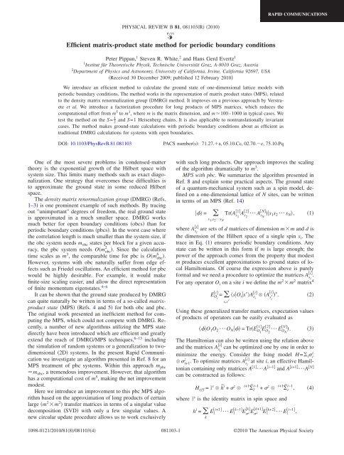
Efficient matrix-product state method for periodic boundary conditions
Efficient matrix-product state method for periodic boundary conditions
Efficient matrix-product state method for periodic boundary conditions

Create successful ePaper yourself
Turn your PDF publications into a flip-book with our unique Google optimized e-Paper software.
<strong>Efficient</strong> <strong>matrix</strong>-<strong>product</strong> <strong>state</strong> <strong>method</strong> <strong>for</strong> <strong>periodic</strong> <strong>boundary</strong> <strong>conditions</strong><br />
Peter Pippan, 1 Steven R. White, 2 and Hans Gerd Evertz 1<br />
1 Institut für Theoretische Physik, Technische Universität Graz, A-8010 Graz, Austria<br />
2 Department of Physics and Astronomy, University of Cali<strong>for</strong>nia, Irvine, Cali<strong>for</strong>nia 92697, USA<br />
Received 30 December 2009; published 12 February 2010<br />
We introduce an efficient <strong>method</strong> to calculate the ground <strong>state</strong> of one-dimensional lattice models with<br />
<strong>periodic</strong> <strong>boundary</strong> <strong>conditions</strong>. The <strong>method</strong> works in the representation of <strong>matrix</strong> <strong>product</strong> <strong>state</strong>s MPS, related<br />
to the density <strong>matrix</strong> renormalization group DMRG <strong>method</strong>. It improves on a previous approach by Verstraete<br />
et al. We introduce a factorization procedure <strong>for</strong> long <strong>product</strong>s of MPS matrices, which reduces the<br />
computational ef<strong>for</strong>t from m5 to m3 , where m is the <strong>matrix</strong> dimension, and m100–1000 in typical cases. We<br />
test the <strong>method</strong> on the S= 1<br />
2 and S=1 Heisenberg chains. It is also applicable to nontranslationally invariant<br />
cases. The <strong>method</strong> makes ground-<strong>state</strong> calculations with <strong>periodic</strong> <strong>boundary</strong> <strong>conditions</strong> about as efficient as<br />
traditional DMRG calculations <strong>for</strong> systems with open boundaries.<br />
DOI: 10.1103/PhysRevB.81.081103 PACS numbers: 71.27.a, 05.10.Cc, 02.70.c, 75.10.Pq<br />
One of the most severe problems in condensed-matter<br />
theory is the exponential growth of the Hilbert space with<br />
system size. This limits many <strong>method</strong>s such as exact diagonalization.<br />
One strategy that overcomes these difficulties is<br />
to approximate the ground <strong>state</strong> in some reduced Hilbert<br />
space.<br />
The density <strong>matrix</strong> renormalization group DMRG Refs.<br />
1–3 is one prominent example of such <strong>method</strong>s. By tracing<br />
out ”unimportant” degrees of freedom, the real ground <strong>state</strong><br />
is approximated in a much smaller space. DMRG works<br />
much better <strong>for</strong> open <strong>boundary</strong> <strong>conditions</strong> obcs than <strong>for</strong><br />
<strong>periodic</strong> <strong>boundary</strong> <strong>conditions</strong> pbcs. In the worst case where<br />
the correlation length is much smaller than the system size, if<br />
the obc system needs mobc <strong>state</strong>s per block <strong>for</strong> a given accu-<br />
2<br />
racy, the pbc system needs Omobc. Since the calculation<br />
time scales as m 3 , the comparable time <strong>for</strong> pbc is Om obc<br />
6 .<br />
However, systems with obc naturally suffer from edge effects<br />
such as Friedel oscillations. An efficient <strong>method</strong> <strong>for</strong> pbc<br />
would be highly desirable. For example, it would make<br />
finite-size scaling easier, and allow the direct representation<br />
of finite momentum eigen<strong>state</strong>s. 4–6<br />
It can be shown that the ground <strong>state</strong> produced by DMRG<br />
can quite naturally be written in terms of a so-called <strong>matrix</strong><strong>product</strong><br />
<strong>state</strong> MPS Refs. 4 and 5 <strong>for</strong> both obc and pbc.<br />
The original work presented an inefficient <strong>method</strong> <strong>for</strong> computing<br />
the MPS, which could not compete with DMRG. Recently,<br />
a number of new algorithms utilizing the MPS <strong>state</strong><br />
directly have been introduced which are efficient and greatly<br />
extend the reach of DMRG/MPS techniques, 6–13 including<br />
the simulation of random systems or a generalization to twodimensional<br />
2D systems. In the present Rapid Communication<br />
we investigate an algorithm presented in Ref. 8 <strong>for</strong> an<br />
MPS treatment of pbc systems. Within this approach m pbc<br />
m obc, a tremendous improvement. However, that algorithm<br />
has a computational cost of m 5 , making the net improvement<br />
modest.<br />
Here we introduce an improvement to this pbc MPS algorithm<br />
based on the approximation of long <strong>product</strong>s of certain<br />
large m 2 m 2 transfer matrices in terms of a singular value<br />
decomposition SVD with only a few singular values. A<br />
new circular update procedure allows us to work exclusively<br />
PHYSICAL REVIEW B 81, 081103R 2010<br />
with such long <strong>product</strong>s. Our approach improves the scaling<br />
of the algorithm dramatically to m3 .<br />
MPS with pbc. We summarize the algorithm presented in<br />
Ref. 8 and explain some practical aspects. The ground <strong>state</strong><br />
of a quantum-mechanical system such as a spin model, defined<br />
on a one-dimensional lattice of N sites, can be written<br />
in terms of an MPS Ref. 14<br />
1 2 N<br />
= TrAs1 As2 ¯ AsN s1s2 ¯ sN, 1<br />
s1 ,s2¯sN i<br />
where Asi are sets of d matrices of dimension mm and d is<br />
the dimension of the Hilbert space of a single spin si. The<br />
trace in Eq. 1 ensures <strong>periodic</strong> <strong>boundary</strong> <strong>conditions</strong>. Any<br />
<strong>state</strong> can be written in this <strong>for</strong>m if m is large enough; the<br />
power of the approach comes from the property that modest<br />
m produces excellent approximations to ground <strong>state</strong>s of local<br />
Hamiltonians. Of course the expression above is purely<br />
i<br />
<strong>for</strong>mal and we need a procedure to optimize the matrices Asi .<br />
For any operator Oi on a site i we define the m2m 2 <strong>matrix</strong>4 i i i EOi = sOisA si Asi<br />
<br />
. 2<br />
s,s<br />
Using these generalized transfer matrices, expectation values<br />
of <strong>product</strong>s of operators can be easily evaluated as<br />
1 2 N<br />
O1O2 ¯ ON =TrEO1EO2¯ EON.<br />
3<br />
The Hamiltonian can also be written using the relation above<br />
i<br />
and the matrices Asi can be optimized one by one in order to<br />
z<br />
minimize the energy. Consider the Ising model H= ii z<br />
i<br />
i+1. To optimize matrices Asi at site i, an effective Hamiltonian<br />
containing only matrices A1 ¯Ai−1 and Ai+1¯A N<br />
can be constructed as follows:<br />
Heff = 1s h ˜i + z i+1 ˜ i−1 z i+1<br />
l + ˜ i−1<br />
r , 4<br />
where 1s is the identity <strong>matrix</strong> in spin space and<br />
h i = k<br />
RAPID COMMUNICATIONS<br />
i+1 k−1 k k+1 k+2 i−1<br />
E1 ¯ E1 Ez Ez E1 ¯ E1 ,<br />
1098-0121/2010/818/0811034 081103-1<br />
©2010 The American Physical Society
PIPPAN, WHITE, AND EVERTZ PHYSICAL REVIEW B 81, 081103R 2010<br />
i+1 i−1 i+1 i+2 i+3 i−1<br />
l = Ez E1 E1 ¯ E1 ,<br />
i+1 i−1 i+1 i+2 i−2 i−1<br />
r = E1 E1 ¯ E1 Ez . 5<br />
In the equation above, all indices are taken modulo N. The<br />
tilde in Eq. 4 refers to the exchange of indices Xijkl =X ˜ ikjl. Together with a map of the identity <strong>matrix</strong> Neff =1s Ñi , Ni i+1 N 1 i−1<br />
=E1 ¯E1 E1 ¯E1 , a new set of d matri-<br />
i<br />
ces Asi <strong>for</strong> fixed i is found by solving the generalized eigenvalue<br />
problem<br />
H eff VecA = N eff VecA, 6<br />
with the expectation value of the energy and VecA the<br />
dm2 i<br />
elements of Asi , aligned to a vector.<br />
When a new set of matrices has been found, the matrices<br />
need to be regauged, in order to keep the algorithm stable. In<br />
DMRG this is not necessary since the basis of each block is<br />
orthogonal. The orthogonality constraint reads as<br />
i i † siAsi Asi =1. It can be satisfied as follows: The <strong>state</strong> is left<br />
l l l,s l+1<br />
unchanged when we substitute As →As XU and As<br />
→X−1 l+1<br />
As , with some nonsingular <strong>matrix</strong> X. This <strong>matrix</strong> X<br />
l<br />
has to be found such that Us obeys the normalization con-<br />
l l † dition sUs Us =1. We obtain X by calculating the in-<br />
l l † verse of the square root of Q= sAs As . Since Q is not<br />
guaranteed to be nonsingular, the pseudoinverse has to be<br />
used, 15 by discarding singular values close to zero in an SVD<br />
i<br />
of Q. Heff can be calculated iteratively, 8 while updating the<br />
A-matrices one site at a time. One sweeps back and <strong>for</strong>th in<br />
a DMRG-like manner.<br />
Vidal introduced a different approach, <strong>for</strong> infinitely long<br />
translationally invariant systems. 11 By assuming only two<br />
different kinds of matrices A1 and A2 and aligning them in<br />
alternating order, an algorithm <strong>for</strong> both ground <strong>state</strong> and time<br />
evolution can be constructed that updates the matrices in<br />
only Om3 steps. However, unlike the <strong>periodic</strong> MPS <strong>method</strong><br />
discussed here, Vidal’s <strong>method</strong> does not apply to nontranslationally<br />
invariant systems e.g., when impurities or a sitedependent<br />
magnetic field are studied. In addition, the <strong>periodic</strong><br />
MPS <strong>method</strong> can be adapted6 to treat excited <strong>state</strong>s,<br />
whereas the <strong>method</strong> of Ref. 11 probably cannot, since the<br />
excitations would be spread over an infinite lattice and would<br />
have no effect on any individual site. Recently, a related<br />
approach came to our attention, 16 in which the E <strong>matrix</strong> of a<br />
translationally invariant system is treated in Om3. Also recently,<br />
related Quantum Monte Carlo variational <strong>method</strong>s using<br />
tensor <strong>product</strong> <strong>state</strong>s were introduced, 12,13 with scaling<br />
ONm3 per Monte Carlo sweep.<br />
Computational efficiency. It was shown in Ref. 8 that the<br />
m needed <strong>for</strong> pbc systems in the MPS approach is comparable<br />
to the m needed in obc systems within DMRG. However,<br />
it is also vital how CPU time scales with m. In efficient<br />
DMRG programs, most operations can be done by computing<br />
multiplications of mm matrices see Ref. 3, Ch. II.i.<br />
In contrast, in the MPS algorithm described above, operations<br />
on m2m 2 matrices need to be done to <strong>for</strong>m the <strong>product</strong>s<br />
of E-matrices that represent the Hamiltonian. So one<br />
would expect the algorithm to be of order Om6. By taking<br />
081103-2<br />
1 l<br />
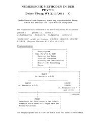
FIG. 1. Color online SVD of a <strong>product</strong> E1 ¯E1 with m<br />
=10. The logarithm of the singular values k is shown <strong>for</strong> different<br />
l in the case of a spin 1 Heisenberg chain of length 100 with <strong>periodic</strong><br />
<strong>boundary</strong> <strong>conditions</strong>. The inset shows data <strong>for</strong> a spin 1<br />
2 Heisenberg<br />
chain.<br />
advantage of the special <strong>for</strong>m of the E matrices Eq. 2,<br />
multiplications can be done in Om 5 which is, however, still<br />
Om 2 slower than DMRG.<br />
Decomposition of <strong>product</strong>s. We now introduce an approximation<br />
in the space of m 2 m 2 matrices which reduces<br />
the CPU time dramatically while the accuracy of the calculation<br />
does not suffer. Let us per<strong>for</strong>m a singular value decomposition<br />
of a long <strong>product</strong> of E matrices<br />
1 2<br />
EO1EO2 ¯ EOl<br />
l T<br />
= kukvk . 7<br />
k=1<br />
It turns out that the singular values k decay very fast.<br />
l<br />
This is shown in Fig. 1 <strong>for</strong> <strong>product</strong>s of the <strong>for</strong>m i=1E1 with<br />
various values of l, <strong>for</strong> the case of the spin 1 Heisenberg<br />
chain. One can see that the longer the <strong>product</strong> the faster the<br />
singular values decay, roughly exponentially in the length l.<br />
We there<strong>for</strong>e propose to approximate long <strong>product</strong>s in a reduced<br />
basis<br />
l<br />
<br />
i=1<br />
p<br />
i<br />
EOi <br />
k=1<br />
m 2<br />
ku kv k T , 8<br />
with p chosen suitably large. In the example of Fig. 1, we<br />
would choose p to be 4 at l=50. Remarkably, <strong>for</strong> longer<br />
<strong>product</strong>s p can be as small as 2 without a detectable loss of<br />
accuracy. Thus, the large distance behavior of the ground<br />
<strong>state</strong> of the spin 1 chain is encoded in these two numbers,<br />
similar to the transfer matrices of a classical spin chain. The<br />
situation does not change significantly when more complicated<br />
operators such as the Hamiltonian are decomposed. Of<br />
course, the decay of the singular values will be model depen-<br />
dent. For a spin 1<br />
2<br />
RAPID COMMUNICATIONS<br />
Heisenberg chain we found that the de-<br />
composition can be done in the same manner with approximately<br />
the same number of singular values to be kept.<br />
A multiplication of a <strong>product</strong> with a new E <strong>matrix</strong> can<br />
there<strong>for</strong>e be done 17 in Opm 3 and a multiplication of two<br />
terms such as Eq. 8 can be done in Oppm 2 . By building
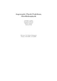
time<br />
10 3<br />
10 2<br />
10 1<br />
36 sites<br />
fit: k = 2.6<br />
60 sites<br />
fit: k = 2.7<br />
100 sites<br />
fit: k = 3.1<br />
20 30 40 50 60 70<br />
m<br />
RAPID COMMUNICATIONS<br />
EFFICIENT MATRIX-PRODUCT STATE METHOD FOR… PHYSICAL REVIEW B 81, 081103R 2010<br />
the effective Hamiltonian out of <strong>product</strong>s in this representation,<br />
the iterative evaluation of the eigenvalue problem can<br />
be accelerated. Whereas in a dense <strong>for</strong>m each <strong>matrix</strong>-vector<br />
multiplication,—which occurs in eigenvalue routines such as<br />
Lanczos or Davidson—takes dm22 operations, it can now<br />
be done in Od2pm2. Note that all operations are now done<br />
on matrices of size mm.<br />
Per<strong>for</strong>ming the SVD in m3 . A crucial step is the efficient<br />
generation of the SVD representation of a large m2m 2 <strong>matrix</strong><br />
M in only Om3 operations. We describe a simple algorithm,<br />
with a fixed number of singular values four to keep<br />
the notation simple. Suppose that M =UdV, with d a44<br />
diagonal <strong>matrix</strong>, and that multiplication of M by a vector<br />
without using the SVD factorization can be done in Om3. To construct U, d, and V with Om3 operations, we first<br />
<strong>for</strong>m a random 4m 2 <strong>matrix</strong> x, and construct y=xM. The 4<br />
rows of y, are linear combinations of the rows of V. Orthonormalize<br />
them to <strong>for</strong>m y. Its rows act as a complete<br />
orthonormal basis <strong>for</strong> the rows of V. This means that V<br />
=VyTy, and thus M =MyTy. Construct z=MyT , and per<strong>for</strong>m<br />
an SVD on z: z=UdV. Then M =zy=UdV, where V<br />
=Vy. V is row orthogonal because V is orthogonal and y<br />
is row orthogonal. The calculation time <strong>for</strong> the orthogonalization<br />
of y and the SVD of z is Om2, and so the calculation<br />
time is dominated by the two multiplications by M, e.g.,<br />
roughly 24Om 3. 18<br />
In applying this approach to the <strong>periodic</strong> MPS algorithm,<br />
M is a <strong>product</strong> of ON E matrices such as in Eq. 5, which<br />
in turn are outer <strong>product</strong>s 2. The multiplication with M can<br />
be done iteratively in ONm3 operations, analogously to the<br />
i<br />
construction of Heff. The calculation time is thus ONm3 <strong>for</strong><br />
each SVD representation generated this way. It is only<br />
needed a few times per sweep see below.<br />
A circular algorithm. A speedup in the simulation can<br />
only be expected if the number of singular values that need<br />
to be included is sufficiently small. However, in the algorithm<br />
of Ref. 8 one sweeps back and <strong>for</strong>th through the lattice,<br />
so that close to the turning points, <strong>product</strong>s of only a few E<br />
matrices appear, which require more singular values Fig. 1.<br />
In the extreme case of only one E <strong>matrix</strong>, we would have<br />
p=m 2 ion, thus making natural use of the <strong>periodic</strong> <strong>boundary</strong> <strong>conditions</strong>.<br />
Note that we cannot employ multiplications with in-<br />
−1<br />
verse matrices EO , since they are too expensive to calculate.<br />
We consider the lattice as a circular ring, and divide it into<br />
thirds, or ”sections.” We per<strong>for</strong>m update steps <strong>for</strong> one section<br />
at a time. To start one section, we first construct the Hamiltonian<br />
and other necessary operators see Eq. 5 corresponding<br />
to the other two sections of the lattice. Only a few<br />
such operators are needed. Each of them contains <strong>product</strong>s of<br />
N/3 E matrices and is computed by an SVD decomposition<br />
as described be<strong>for</strong>e.<br />
Then a set of these operators is made by successively<br />
adding sites from the right most part of the current section to<br />
the operators constructed <strong>for</strong> the section on the right, working<br />
one’s way to the left. Adding a site involves the multiplication<br />
of an E-<strong>matrix</strong> to the left of an operator. These steps<br />
can each be done in Om<br />
. To overcome this bottleneck we propose a modified<br />
<strong>method</strong> which proceeds through the chain in a circular fash-<br />
3 operations. When one has<br />
reached the left side of the current section, its initialization is<br />
finished and one can start the normal update steps, now<br />
building up a set of operators from the left, again in Om3 operations. One stops when one reaches the right-hand side<br />
of the current section. Then the procedure repeats with the<br />
section to the right as the new current section. Some of the<br />
operators previously computed can be reused. The updates<br />
now go in a circular pattern rather than the usual back and<br />
<strong>for</strong>th.<br />
By proceeding in this way on a system of length N, the<br />
blocks on which we have to per<strong>for</strong>m an SVD are of length at<br />
least N/3 if we split our system into three parts, so that the<br />
SVD will have only few singular values. Consequently, the<br />
algorithm is expected to scale like ONm3. Test and results. To test our improvements, we studied<br />
spin 1 and spin 1<br />
FIG. 2. Color online Scaling of the circular version of the<br />
algorithm. CPU time per sweep one update of each site is measured<br />
on a 100 site spin<br />
2 Heisenberg chains up to length N=100.<br />
The exact ground-<strong>state</strong> energy <strong>for</strong> pbc on an N=100 chain in<br />
the spin 1 case is found to be E0/N−1.401 484 038 65<br />
via a DMRG calculation with m=2000. The error is generously<br />
estimated from the truncation error and an extrapolation<br />
in m. The <strong>periodic</strong> result differs from the infinite system<br />
1<br />
2 Heisenberg chain <strong>for</strong> different system<br />
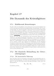
sizes. The time is fitted to a function mk . FIG. 3. Color online Relative error of the ground-<strong>state</strong> energy<br />
of the spin 1 Heisenberg model versus the dimension m of the<br />
reduced Hilbert space. DMRG results with obc and pbc are shown,<br />
as well as Matrix Product State results with pbc. The inset shows<br />
MPS results with pbc <strong>for</strong> a spin 1<br />
2 Heisenberg chain of 100 sites.<br />
081103-3
PIPPAN, WHITE, AND EVERTZ PHYSICAL REVIEW B 81, 081103R 2010<br />
result determined using long open chains only in the last<br />
decimal place, so we will call this value “exact.”<br />
We discarded singular values smaller than a 10 −11 th of the<br />
largest one. This parameter is chosen such that the algorithm<br />
remains stable, which is not the case if the error bound is<br />
chosen too large 10 −8 or larger. To decrease the time it<br />
takes until convergence is reached, we start our calculation<br />
with small m and enlarge it after the algorithm converged <strong>for</strong><br />
the current m. This is also done in many DMRG programs.<br />
We enlarge the matrices A and increase their rank by filling<br />
the new rows and columns with small random numbers r,<br />
uni<strong>for</strong>mly distributed in the interval −10 −6 ,10 −6 . The number<br />
of sweeps it takes until convergence is reached is similar<br />
to DMRG. For the present model, two or three sweeps are<br />
enough <strong>for</strong> each value of m.<br />
Figure 2 shows that the algorithm indeed scales like m 3 ,<br />
and no longer like m 5 . It is slightly faster on small systems,<br />
due to faster parts of the algorithm, and becomes slightly<br />
slower on large systems, likely due to memory access times.<br />
Our <strong>method</strong> on a <strong>periodic</strong> system requires a constant factor<br />
of about 10 as many operations per iteration as DMRG does<br />
on an open system, which is still very efficient.<br />
Finally, we studied the convergence to the exact ground<strong>state</strong><br />
energy as a function of m. We investigated DMRG with<br />
obc and pbc, and the MPS algorithm with pbc, both the<br />
original version and our improved <strong>method</strong>. The relative error<br />
<strong>for</strong> these cases is plotted in Fig. 3. The relative error of<br />
E<br />
E 0<br />
1S. R. White, Phys. Rev. Lett. 69, 2863 1992.<br />
2S. R. White, Phys. Rev. B 48, 10345 1993.<br />
3U. Schollwöck, Rev. Mod. Phys. 77, 259 2005.<br />
4S. Östlund and S. Rommer, Phys. Rev. Lett. 75, 3537 1995.<br />
5S. Rommer and S. Östlund, Phys. Rev. B 55, 2164 1997.<br />
6D. Porras, F. Verstraete, and J. I. Cirac, Phys. Rev. B 73, 014410<br />
2006.<br />
7G. Vidal, Phys. Rev. Lett. 91, 147902 2003.<br />
8F. Verstraete, D. Porras, and J. I. Cirac, Phys. Rev. Lett. 93,<br />
227205 2004.<br />
9B. Paredes, F. Verstraete, and J. I. Cirac, Phys. Rev. Lett. 95,<br />
140501 2005.<br />
10F. Verstraete and J. Cirac, arXiv:cond-mat/0407066 unpublished.<br />
081103-4<br />
RAPID COMMUNICATIONS<br />
the spin correlation function not shown is of similar magnitude<br />
with our improved <strong>method</strong>.<br />
As has been well known, DMRG with obc per<strong>for</strong>ms much<br />
better than with pbc. With the MPS algorithm and pbc the<br />
relative error as a function of m is comparable to the error<br />
made with DMRG and obc. This has already been reported<br />
earlier. 8 The important point here is that the error remains the<br />
same when we introduce the approximations. Also, the number<br />
of sweeps until convergence is reached is similar <strong>for</strong><br />
DMRG with obc and <strong>for</strong> MPS. We note that the convergence<br />
in Fig. 3 is consistent with exponential behavior in the spin 1<br />
case and with a power law <strong>for</strong> spin 1<br />
2 .<br />
In a typical DMRG calculation, <strong>matrix</strong> dimensions m<br />
100–1000 and larger are used. To illustrate the computational<br />
time scaling, suppose we study a model which requires<br />
m=300 <strong>state</strong>s <strong>for</strong> obc with traditional DMRG. Then<br />
our approach gains a factor of roughly m5 /m3 105 over the<br />
<strong>method</strong> of Ref. 8, and even more over traditional DMRG.<br />
In summary, by introducing a well-controlled approximate<br />
representation of <strong>product</strong>s of MPS transfer matrices in terms<br />
of a singular value decomposition, we have <strong>for</strong>mulated a<br />
circular MPS <strong>method</strong> <strong>for</strong> systems with <strong>periodic</strong> <strong>boundary</strong><br />
<strong>conditions</strong>, which works with a computational ef<strong>for</strong>t comparable<br />
to that of DMRG with open <strong>boundary</strong> <strong>conditions</strong>.<br />
We acknowledge support from the NSF under Grant No.<br />
DMR-0605444 S.R.W. and from NAWI Graz P.P..<br />
11G. Vidal, Phys. Rev. Lett. 98, 070201 2007.<br />
12N. Schuch, M. M. Wolf, F. Verstraete, and J. I. Cirac, Phys. Rev.<br />
Lett. 100, 040501 2008.<br />
13A. W. Sandvik and G. Vidal, Phys. Rev. Lett. 99, 220602 2007.<br />
14D. Perez-Garcia, F. Verstraete, M. Wolf, and J. Cirac, Quantum<br />
Inf. Comput. 7, 401 2007.<br />
15F. Verstraete private communication.<br />
16F. Verstraete et al. unpublished.<br />
17 2 Denote v as an m vector and V as the elements of v aligned as<br />
an mm <strong>matrix</strong>. Then one can use the relation A Bv<br />
=VecBVAT to per<strong>for</strong>m a <strong>matrix</strong>-vector <strong>product</strong>.<br />
18A Lanczos approach would take an additional factor <strong>for</strong> convergence.