† 9.1.1.1 Fourier Series and the Gibb's Phenomenon. Fejer Sum

† 9.1.1.1 Fourier Series and the Gibb's Phenomenon. Fejer Sum
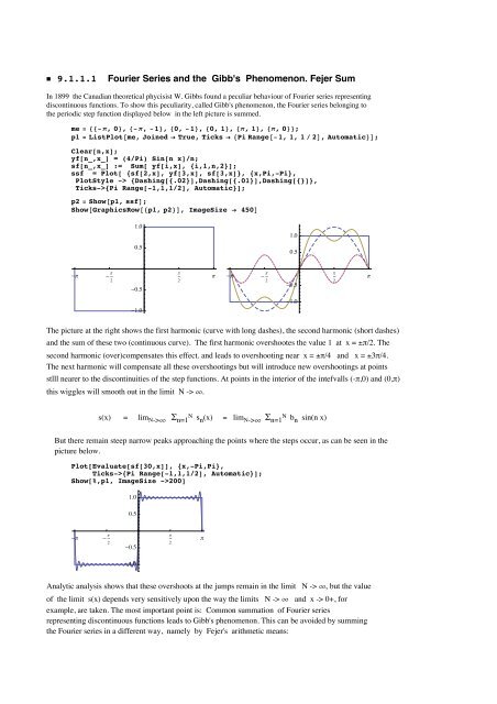
In 1899 the Canadian theoretical phycisist W. Gibbs found a peculiar behaviour of Fourier series representing
discontinuous functions. To show this peculiarity, called Gibb's phenomenon, the Fourier series belonging to
the periodic step function displayed below in the left picture is summed.
me = 88-p, 0 and x -> 0+, for
example, are taken. The most important point is: Common summation of Fourier series
representing discontinuous functions leads to Gibb's phenomenon. This can be avoided by summing
the Fourier series in a different way, namely by Fejer's arithmetic means:
s(x) = lim N-> Σ n=1 N σn (x),
2
1.0
0.5
-0.5
-1.0
σ n (x) = n -1 Σ i=1 n si (x) = n -1 Σ i=1 n k=1 i bk sin(k x)
p
2
p

2 K9GibbsPhenomenon.nb
s(x) = lim N-> Σ n=1 N σn (x),
σ n (x) = n -1 Σ i=1 n si (x) = n -1 Σ i=1 n k=1 i bk sin(k x)
sff[n_,x_] := Sum[ sf[i,x], {i,n}]/n ;
Plot[Evaluate[{sff[2,x], sf[3,x], sff[3,x]}], {x,Pi,-Pi},
PlotStyle -> {Dashing[{.02}],Dashing[{.01}],Dashing[{}]},
Ticks -> {Pi Range[-1,1,1/2],Automatic}];
ss3 = Show@p1, %D;
Plot[Evaluate[sff[20,x]], {x,Pi,-Pi}];
ss0 = Show[p1, %, Ticks -> {Pi Range[-1,1,1/2],Automatic} ];
Show[GraphicsRow[{ss3,ss0}], ImageSize Ø 450]
-p - p
2
1.0
0.5
-0.5
-1.0
p
2
p
-p - p
2
1.0
0.5
-0.5
-1.0
p
2
p