Basics of Polarizing Microscopy - Olympus
Basics of Polarizing Microscopy - Olympus
Basics of Polarizing Microscopy - Olympus

You also want an ePaper? Increase the reach of your titles
YUMPU automatically turns print PDFs into web optimized ePapers that Google loves.
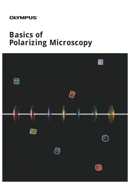
<strong>Basics</strong> <strong>of</strong><br />
<strong>Polarizing</strong> <strong>Microscopy</strong>
KEYWORD<br />
Polarized light<br />
Linearly polarized light<br />
Circularly polarized light<br />
Elliptically polarized light<br />
<strong>Polarizing</strong> plate<br />
<strong>Polarizing</strong> filter<br />
<strong>Polarizing</strong> prism<br />
Polarizer<br />
Analyzer<br />
Crossed nicols<br />
Parallel nicols<br />
1.Properties <strong>of</strong> polarized light<br />
1.1 Polarized light<br />
Transverse wave light whose vibration possess<br />
direction is called polarized light. Light from an<br />
ordinary light source (natural light) that vibrates in<br />
random directions (Fig. 1.1) is called nonpolarized<br />
light. In contrast, while light with vertical vibration<br />
that travels within a single plane (Fig. 1.2a) is called<br />
linearly polarized light, circularly polarized light (Fig.<br />
1.2b) and elliptically polarized light (Fig. 1.2c) are<br />
types <strong>of</strong> light in which the vibration plane rotates<br />
forward.<br />
Fig. 1.2 Types <strong>of</strong> polarized light<br />
A polarizing plate (polarizing filter) or polarizing<br />
prism is <strong>of</strong>ten used as the device to change natural<br />
light to linearly polarized light (see 1.7).<br />
Configuring the primary and secondary polarizing<br />
devices in the orthogonal directions <strong>of</strong> each<br />
transmitting linearly polarized ray will cut the light.<br />
Such state in which the primary light polarizing<br />
device is the polarizer and the secondary device<br />
is the analyzer is called crossed nicols. Parallel<br />
nicols is the state in which the analyzer is rotated<br />
to make the direction <strong>of</strong> the transmitting linearly<br />
polarized light match with the polarizer, and the<br />
amount <strong>of</strong> light transmittance is maximized. (Fig.<br />
1.3b).<br />
1<br />
The vibration direction <strong>of</strong> light is perpendicular to<br />
the progressing light. The vibration direction <strong>of</strong><br />
natural light points to all the directions.<br />
Fig. 1.1 Natural light (nonpolarized light)<br />
a. linearly polarized light b. circularly polarized light c. elliptically polarized light<br />
Each figure on the left-hand side shows decomposition <strong>of</strong> each polarized light into two mutual<br />
perpendicular linearly polarized light.<br />
Fig. 1.3 a) crossed nicols and b) parallel nicols<br />
P: polarizer A: analyzer
1.2 Polarization by reflection<br />
When light reflects <strong>of</strong>f the surface <strong>of</strong> water and<br />
glass, its reflectance varies with the direction <strong>of</strong><br />
polarization (Fig. 1.4a). Comparing the two oscillation<br />
components, Component P is parallel to the<br />
plane <strong>of</strong> incidence and has 0 reflectance while<br />
Component S is perpendicular to the plane and<br />
has higher reflectance. The 0 reflectance <strong>of</strong><br />
Component P is caused by the existence <strong>of</strong> an<br />
angle <strong>of</strong> incidence, known as the Brewster angle.<br />
In other words, the reflected light at this angle is<br />
linearly polarized, and can be cut out with a polarizing<br />
plate. In photography, a polarizing filter is<br />
used in order to remove reflection from the surface<br />
<strong>of</strong> water and glass (Fig. 1.4b). The Brewster<br />
angle against the surface <strong>of</strong> water (n=1.33) and<br />
the surface <strong>of</strong> glass (n=1.52) is 53°07' and 56°40',<br />
respectively.<br />
1.3 Double refraction<br />
An object whose image passes through a calcite<br />
CaCO3 crystal appears doubled (Fig. 1.5a). This<br />
phenomenon is called double refraction or birefringence,<br />
which occurs when light that is<br />
launched through a crystal material is divided into<br />
two linearly polarized light rays having mutually<br />
crossing vibration directions, and then refracted.<br />
Among these two light rays, the one that follows<br />
the law <strong>of</strong> refraction is called an ordinary ray, while<br />
the other one is called an extraordinary ray. Their<br />
speed and index <strong>of</strong> refraction differ from one<br />
another.<br />
A crystal that refracts in such way is called an<br />
anisotropy. Light passing through an anisotropy is<br />
generally divided into ordinary and extraordinary<br />
rays, but toward a certain direction called optical<br />
axis, they travel together. When that happens, the<br />
double refraction phenomenon does not occur.<br />
(see 1.4).<br />
2<br />
tanq1=n<br />
q1: Brewster angle<br />
Fig. 1.4 a) Difference <strong>of</strong> reflectance is due to vibration direction <strong>of</strong> light<br />
b) Effectiveness <strong>of</strong> polarizing filter (left: without filter right: with filter)<br />
Fig. 1.5a. Double refraction phenomenon due to calcite<br />
Ejection light <strong>of</strong><br />
linearly light<br />
Air<br />
Calcite<br />
Extra<br />
ordinary<br />
ray<br />
reflective<br />
indey<br />
: Angle <strong>of</strong> incidence<br />
Ejection ray <strong>of</strong><br />
linearly polarized<br />
light<br />
ordinary<br />
ray<br />
C : optical axis<br />
Fig. 1.5b. Double refraction phenomenon due to diagram<br />
KEYWORD<br />
Component P<br />
Component S<br />
Brewster angle<br />
Calcite<br />
Double refraction<br />
Ordinary ray<br />
Extra ordinary ray<br />
Anisotropy<br />
Optical axis
KEYWORD<br />
Optically uniaxial crystal<br />
Optically biaxial crystal<br />
Principal section<br />
Optically positive crystal<br />
Optically negative crystal<br />
Optical character<br />
Index surface<br />
Principal refractive<br />
1.4 Optically uniaxial crystal<br />
Anisotropy can be divided into an optically uniaxial<br />
crystal and an optically biaxial crystal accordinng<br />
to the optical properties. An optically uniaxial crystal<br />
has one optical axis while an optically biaxial<br />
crystal has two axes. A material classification in<br />
terms <strong>of</strong> optical properties is as follows:<br />
The optical axis and the direction <strong>of</strong> a beam <strong>of</strong><br />
light determine the vibration direction <strong>of</strong> extraordinary<br />
and ordinary rays in an optically uniaxial crystal,<br />
and the section containing both rays is called<br />
the principal section. The ordinary rays oscillate<br />
vertically through the principal section while the<br />
extraordinary rays oscillate within the principal<br />
section (Fig. 1.6).<br />
Optically uniaxial crystals can be divided into two types:<br />
optically positive crystals, in which the index <strong>of</strong> refraction<br />
<strong>of</strong> extraordinary rays is greater than that <strong>of</strong> ordinary rays,<br />
and vice versa, called optically negative crystals<br />
(hereafter, positive crystals and negative crystals). For<br />
instance, rock crystals belong to positive crystals,<br />
whereas calcite and sapphires belong to negative<br />
crystals. Positive and negative crystals can also be said to<br />
possess a positive or negative optical character,<br />
respectively.<br />
The index <strong>of</strong> refraction <strong>of</strong> extraordinary rays varies with<br />
the direction <strong>of</strong> progression <strong>of</strong> light rays. Figure 1.7 shows<br />
the index surface for optically uniaxial crystals with a) a<br />
positive crystal, and b) a negative crystal. The index<br />
surface expresses the index <strong>of</strong> refraction toward the<br />
direction <strong>of</strong> progression <strong>of</strong> ordinary rays and extraordinary<br />
rays in terms <strong>of</strong> the distance from the origin. As shown in<br />
the diagram, the index <strong>of</strong> refraction <strong>of</strong> extraordinary rays<br />
inclined by q from the optical axis is ne. The index <strong>of</strong><br />
refraction <strong>of</strong> extraordinary rays reaches a maximum or<br />
minimum perpendicularly along the direction <strong>of</strong> the optical<br />
axis. The indices <strong>of</strong> refraction <strong>of</strong> the ordinary and<br />
extraordinary rays in this direction, w and e, respectively,<br />
are called principal refractive indices. The principal<br />
refracive indices for significant crystals are given in table<br />
1.1.<br />
3<br />
optically isotropic<br />
body<br />
optically anisotropy<br />
non-crystal<br />
isoaxial system crystal<br />
optically uniaxial crystal<br />
optically biaxial crystal<br />
tetragonal system crystal<br />
hexagonal system crystal<br />
rhombic system crystal<br />
monoclinic system crystal<br />
triclinic system crystal<br />
Fig. 1.6 Vibration direction <strong>of</strong> ordinary rays and extraordinary rays <strong>of</strong> an optically uniaxial crystal<br />
Fig. 1.7 Index surface <strong>of</strong> an optically uniaxial crystal<br />
Crystal name<br />
rock crystal (quartz)<br />
calcite<br />
sapphire<br />
•: vibration direction <strong>of</strong><br />
ordinary ray<br />
(perpendicular to<br />
principal section)<br />
- : vibration direction <strong>of</strong><br />
extra ordinary ray<br />
(within principal section)<br />
The principal section<br />
is surface <strong>of</strong> space.<br />
c : optical<br />
axis<br />
a. positive crystal b. negative crystal<br />
(The ellipse is exaggerated)<br />
1.5443<br />
1.6584<br />
1.768<br />
1.5534<br />
1.4864<br />
1.760<br />
Table 1.1 Principal refractive indices <strong>of</strong> significant crystals (wavelength = 589.3 nm)
In double refraction, the vibration direction <strong>of</strong> light with<br />
faster progression is called the X' direction, while the<br />
slower progression is called the Z' direction. As for the<br />
vibration direction, the positive crystals represent the<br />
direction <strong>of</strong> extraordinary rays, whereas the negative<br />
crystals express that <strong>of</strong> the ordinary rays in the<br />
Z'direction <strong>of</strong> optically uniaxial crystals. In the test plate<br />
and compensator <strong>of</strong> a polarizing microscope (see 3.2.8),<br />
the Z' direction is displayed for investigating the vibration<br />
direction <strong>of</strong> the light for specimens. Generally, even optically<br />
biaxial crystal will separate in two rays, and yet they<br />
are both extraordinary rays whose speed differs according<br />
to the direction <strong>of</strong> its progression. See Fig. 1.8 for the<br />
index surface <strong>of</strong> optically biaxial crystals. a, b, and g show<br />
the principal refractive indices <strong>of</strong> optically biaxial crystals.<br />
The angle that constitutes the two optical axes (2 ) is<br />
called the optical axial angle.<br />
1.5 Retardation<br />
After being launched into an anisotropy. phase<br />
differences will occur between the ordinary and<br />
extraordinary rays. Fig. 1.9 shows the relationship<br />
between the direction <strong>of</strong> the optical axis and double<br />
refraction. In cases (a) and (b) in Fig. 1.9, relative<br />
surges and delays, i.e., phase differences, d,<br />
will occur between the two rays. On the contrary,<br />
no phase difference can be seen in Fig. 1.9c<br />
because light rays advance in the direction <strong>of</strong> the<br />
optical axis.<br />
The phase difference for extraordinary and ordinary<br />
rays after crystal injection is given next.<br />
(1.1)<br />
l indicates the light wavelength, d the thickness <strong>of</strong><br />
double refraction properties. ne and no are the<br />
refraction indices <strong>of</strong> extraordinary and ordinary<br />
rays, respectively.<br />
Here, the optical path difference R is called retardation<br />
and can be expressed as follows.<br />
(1.2)<br />
R is the value <strong>of</strong> the deviation <strong>of</strong> two light rays in a<br />
double refraction element, converted to mid-air<br />
distance; it is expressed in a direct number (147<br />
nm, etc.), a fraction or the multiple<br />
( /4, etc.) <strong>of</strong> the used wavelength.<br />
4<br />
1.Properties <strong>of</strong> polarized light<br />
OP : Direction <strong>of</strong><br />
optical axis<br />
2 : optical axial<br />
angle<br />
Direction <strong>of</strong> arrows express the<br />
vibration direction.<br />
Fig. 1.8 Section <strong>of</strong> refractive index <strong>of</strong> an optically biaxial crystal<br />
o : ordinary ray<br />
e : extraordinary<br />
ray<br />
: Direction <strong>of</strong><br />
optical axis<br />
Fig. 1.9 Relationship between direction <strong>of</strong> optical axis and double refraction <strong>of</strong> a crystal<br />
KEYWORD<br />
X' direction<br />
Z' direction<br />
Optical axial angle<br />
Phase difference<br />
Retardation
KEYWORD<br />
Optical strain<br />
Photoelasticity<br />
Dichroism<br />
Glan-Thompson prism<br />
Nicol prism<br />
1.6 Optical strain<br />
When stress is applied to an isotropic body such<br />
as glass or plastic, optical strain occurs, causing<br />
the double refraction phenomenon, and that is<br />
called photoelasticity. By observing the optical<br />
strain <strong>of</strong> various materials by means <strong>of</strong> polarization,<br />
the stress distribution can be estimated (Fig.<br />
1.10).<br />
1.7 Light polarizing devices<br />
As stated in 1.2, a polarizing plate and polarizing prism are<br />
generally used as the polarizing devices to convert natural<br />
light into linearly polarized light. Their respective features<br />
are given below.<br />
(1) polarizing plate<br />
A polarizing plate is a piece <strong>of</strong> film by itself or a film<br />
being held between two plates <strong>of</strong> glass. Adding salient<br />
iodine to preferentially oriented macromolecules will<br />
allow this film to have dichroism. Dichroism is a phenomenon<br />
in which discrepancies in absorption occur<br />
due to the vibration direction <strong>of</strong> incident light polarization.<br />
Since the polarizing plate absorbs the light oscillating<br />
in the arranged direction <strong>of</strong> the macromolecule,<br />
the transmitted light rays become linearly polarized.<br />
Despite its drawbacks <strong>of</strong> 1) limited usable wavelength<br />
band (visible to near infrared light), and 2) susceptibility<br />
to heat, the polarizing plate is inexpensive and is easy<br />
to enlarge.<br />
(2) polarizing prism<br />
When natural light is launched into a crystal having<br />
double refraction, the light proceeds in two separate,<br />
linearly polarized lights. By intercepting one <strong>of</strong> these<br />
two, the linearly polarized light can be obtained; this<br />
kind <strong>of</strong> polarizing device is called a polarizing prism,<br />
and among those we find Glan-Thompson prism (a)<br />
and Nicol prism (b).<br />
A polarizing prism has higher transmittance than a<br />
polarizing plate, and provides high polarization characteristics<br />
that cover a wide wavelength band. However,<br />
its angle <strong>of</strong> incidence is limited and it is expensive. In<br />
addition, when used in a polarizing microscope, this<br />
prism takes up more space than a polarizing plate and<br />
may cause image deterioration when placed in an<br />
image forming optical system. For these reasons, a<br />
polarizing plate is generally used except when brightness<br />
or high polarization is required.<br />
5<br />
1.Properties <strong>of</strong> polarized light<br />
Fig. 1.10 Optical strain <strong>of</strong> plastic<br />
express direction <strong>of</strong><br />
optical axis<br />
Fig. 1.11 <strong>Polarizing</strong> prism )<br />
(a. Glan-Thompson prism b. Nicol prism)
2.Fundamentals <strong>of</strong> polarized light analysis<br />
2.1 Anisotropy in crossed nicols<br />
Light does not transmit in a crossed nicols state,<br />
but inserting an anisotropy between a polarizer<br />
and an analyzer changes the state <strong>of</strong> the polarized<br />
light, causing the light to pass through. When<br />
the optical axis <strong>of</strong> a crystal with difference <strong>of</strong> d is<br />
placed between the crossed nicols at an angle <strong>of</strong><br />
q to the polarizer's vibration direction, the intensity<br />
<strong>of</strong> the injected light is expressed as (2.1).<br />
(2.1)<br />
Io is the intensity <strong>of</strong> transmitted light during parallel<br />
nicols, and R is the retardation (equation (1.2)).<br />
With this equation, the change in brightness during<br />
the rotation <strong>of</strong> an anisotropy and <strong>of</strong> the interference<br />
color from retardation can be explained.<br />
As the equation 2.1 signifies, at certain four positions,<br />
(90 degrees apart from each other), the<br />
anisotropy appears black as its optical axis<br />
matches with or becomes perpendicular to the<br />
vibration direction. Such positions are called the<br />
extinction positions. The brightest position, also<br />
known as the diagonal position, is at a 45°. The<br />
drawings in Fig. 2.2 represent the change in<br />
brightness from extinct to diagonal position and<br />
vice versa, while rotating the body.<br />
6<br />
polarizer<br />
anisotropy<br />
Fig. 2.1 Anisotropy between crossed nicols<br />
2.1.1 Change in brightness when rotating anisotropy<br />
analyzer<br />
A : direction <strong>of</strong> progression <strong>of</strong> analyzer<br />
P : direction <strong>of</strong> progression <strong>of</strong> polarizer<br />
C : direction <strong>of</strong> optical axis <strong>of</strong> anisotropy<br />
A : vibration direction<br />
<strong>of</strong> analyzer<br />
P : vibration direction<br />
<strong>of</strong> polarizer<br />
Fig. 2.2 Extinction position and diagonal position <strong>of</strong> anisotropy<br />
KEYWORD<br />
Extinction position<br />
Diagonal position
KEYWORD<br />
Interference color<br />
Interference color chart<br />
The first order<br />
Sensitive color<br />
2.1.2 Interference color in anisotropy<br />
By equation (2.1), when the phase difference d <strong>of</strong> an<br />
anisotropy is 0, 2 , 4 , (retardation R 0, , 2 ,<br />
…, represents a single color wavelength) the intensity<br />
<strong>of</strong> the transmitted light is 0, or the body appears<br />
pitch dark. On the other hand, when the body seems<br />
brightest, d is p, 3p, 5p,. (R is /2, 3 /2, 5 /2,<br />
…)This gap in light intensity attributes to the phase difference<br />
created between the ordinary and extraordinary<br />
rays after passing through an anisotropy, next<br />
through an analyzer, and eventually to have interference.<br />
Fig. 2.3 shows the transmittance <strong>of</strong> light when a<br />
wedge-shaped quartz plate, having double refraction is<br />
placed in the diagonal position in crossed nicols. In the<br />
case <strong>of</strong> single color light, the intensity <strong>of</strong> transmitted<br />
light creates light and dark fringes. As the phase difference<br />
<strong>of</strong> an ordinary and extraordinary rays vary according<br />
to the wavelength, so does the transmittance at<br />
each wavelength. (See formula 1.1).<br />
When observing the wedge-shaped quartz plate <strong>of</strong> Fig.<br />
2.3 under white light, interference destroys some<br />
wavelengths and reinforce others. As a result, by<br />
superimposing the wavelength <strong>of</strong> visible light, the color<br />
appears. This is called interference color.<br />
Fig. 2.4 Color Chart<br />
The visible colors in the color chart from zero order<br />
black to first order purplish-red are called the first order<br />
colors. The first order purplish-red is extremely vivid,<br />
and the interference color changes from yellow, red to<br />
blue just by the slightest retardation. This purplish-red is<br />
called a sensitive color. Colors between the first order<br />
7<br />
(Transmitted light intensity)<br />
=486nm<br />
(blue)<br />
=546nm<br />
(green)<br />
=656nm<br />
(red)<br />
wedge-shaped<br />
quartz plate<br />
expresses the direction<br />
<strong>of</strong> optical axis<br />
R(retardation)<br />
Fig. 2.3 Transmittance <strong>of</strong> wedge-shaped quartz plate<br />
The relationship between retardation amount <strong>of</strong><br />
anisotropy and interference color is shown by the<br />
interference color chart. By comparing the interference<br />
color <strong>of</strong> the anisotropy with the interference<br />
color chart, the retardation <strong>of</strong> the anisotropy can be<br />
estimated. A vertical line is drawn on the interference<br />
color chart to show the relationship between<br />
double refraction (ne-no) and the thickness <strong>of</strong><br />
anisotropy. This is used to find out the thickness d<br />
<strong>of</strong> specimens or the double refraction (ne-no). from<br />
retardation.<br />
red and second order red are called second order<br />
colors, such as second order blue, second order<br />
green. The higher the order <strong>of</strong> colors gets, the<br />
closer the interference color approaches white.
Figure 2.5 shows the transmittance curve <strong>of</strong> the<br />
interference color in relation to retardation around<br />
the sensitive color, and is calculated from equation<br />
(2.1). In the sensitive colors, green light cannot<br />
be transmitted and thus appears as purplishred<br />
(Fig. 2.5b). If retardation is reduced from<br />
sensitive colors, then a wide-range mixed color<br />
light from green to red turns up, observed as yellow,<br />
as shown in Fig. 2.5a; increased retardation,<br />
contrarily, brings out a blue interference color.<br />
(Fig. 2.5c.)<br />
2.2 Superimposing anisotropy<br />
Now we consider two anisotropy overlapping one<br />
another; one with the vibration directions <strong>of</strong> their<br />
slower light rays (Z' direction) in the same direction<br />
(Fig. 2.6a), and the other perpendicularly. (Fig.<br />
2.6b).<br />
When the Z' directions <strong>of</strong> two anisotropy overlap,<br />
pointing the same direction, the vibration directions<br />
<strong>of</strong> the slower polarized light match. The total<br />
retardation is equivalent to the numerical sum <strong>of</strong><br />
the retardations.<br />
R=R1+R2 (R1, R2 denote the retardations <strong>of</strong> anisotropy 1 and 2)<br />
This state is called addition (Fig 2.5a). In contrast<br />
the phase difference after passing through one<br />
anisotropic element is cancelled out by the other<br />
phase difference. As a result, the total retardation<br />
is the difference between the two anisotropy<br />
retardation.<br />
R=R1-R2.<br />
This state is called subtraction (Fig 2.5b). Whether<br />
the state is addition or subtraction can be deter-<br />
2.Fundamentals <strong>of</strong> polarized light analysis<br />
8<br />
a) R=400 nm<br />
The light within the range from green<br />
to purple is transmitted, and appears<br />
yellow with a mixed color.<br />
b) R=530 nm (sensitive color)<br />
The low number <strong>of</strong> green portions<br />
results in purple and red light to<br />
transmit, and is seen as purplish red.<br />
c) R=650 nm<br />
The strong transmitting light <strong>of</strong> blue<br />
and purple emphasizes the blue<br />
color.<br />
Fig. 2.5 Retardation and transmittance curve<br />
Fig. 2.6 Superimposing anisotropy<br />
a:addition b:subtraction<br />
mined from the changes in the interference<br />
color when the anisotropy overlap. Shifting <strong>of</strong><br />
the interference color toward the increase <strong>of</strong><br />
retardation is addition, and vice versa for subtraction.<br />
Both addition and subtraction are the<br />
determinants for judging Z' direction. (To be<br />
discussed further in 4.1.3) Knowing the Z'<br />
direction helps determine the optical character<br />
<strong>of</strong> elongation (see 2.3) In addition, when the<br />
anisotropy overlap with one at the extinction<br />
position and the other at the diagonal position,<br />
the total retardation becomes equivalent to<br />
the retardation <strong>of</strong> the anisotropy at the diagonal<br />
position.<br />
KEYWORD<br />
Addition<br />
Subtraction
KEYWORD<br />
Optical character <strong>of</strong> elongation<br />
Slow length<br />
Fast length<br />
Phase plate<br />
Tint plate<br />
Quarter-wave plate<br />
Half-wave plate<br />
Mica<br />
2.3 Optical character <strong>of</strong> elongation<br />
Some anisotropy are elongated in some direction as the<br />
narrow crystals and fibers in rock would be. The relationship<br />
between the direction <strong>of</strong> elongation and Z' direction<br />
can specify the optical character <strong>of</strong> elongation (zone<br />
character). When the Z' direction matches the direction <strong>of</strong><br />
elongation, it is said to have a slow length, and when the<br />
z' direction crosses the direction <strong>of</strong> elongation, then it has<br />
a fast length).<br />
This optical character does not coincide with the positive<br />
and negative attributes <strong>of</strong> uniaxial and biaxial crystals. The<br />
optical character <strong>of</strong> elongation is fixed for anisotropy such<br />
as crystals (e.g., uric acid sodium crystals <strong>of</strong> gout), and, by<br />
using a polarizing microscope, can be distinguished from<br />
pseudo gout crystals (see 4.1.3).<br />
2.4 Phase plate<br />
A phase plate is used in the conversion <strong>of</strong> linearly<br />
polarized light and circularly polarized light, and in<br />
the conversion <strong>of</strong> the vibration direction <strong>of</strong> linearly<br />
polarized light. A phase plate is an anisotropy which<br />
generates a certain fixed amount <strong>of</strong> retardation, and<br />
based on that amount, several types <strong>of</strong> phase plate<br />
linearly polarized light<br />
circularly polarized light<br />
A half-wave plate is mainly used for changing the<br />
vibration direction <strong>of</strong> linearly polarized light, and for<br />
reversing the rotating direction <strong>of</strong> circularly polarized<br />
and elliptically polarized light. Quarter-wave<br />
2.Fundamentals <strong>of</strong> polarized light analysis<br />
1/4 wave plate<br />
1/4 wave plate<br />
9<br />
direction <strong>of</strong> elongation<br />
optical character <strong>of</strong><br />
elongation is positive<br />
anisotrophy<br />
optical character <strong>of</strong><br />
elongation is negative<br />
Fig. 2.7 Optical character <strong>of</strong> elongation<br />
(tint plate, quarter-wave plate, and half-wave<br />
plate) are made. When using a quarter-wave<br />
plate, a diagonally positioned optical axis<br />
direction can convert incident linearly polarized<br />
light into circularly polarized light and vice versa<br />
(Fig. 2.8).<br />
circularly polarized light<br />
Conversion <strong>of</strong> linearly polarized light into circularly polarized light<br />
linearly polarized light<br />
Conversion <strong>of</strong> circularly polarized light into linearly polarized light<br />
Fig. 2.8 Quarter-wave plate conversion <strong>of</strong> linearly polarized light into circularly polarized light<br />
plates, half-wave plates, and tint plates are<br />
usually thin pieces <strong>of</strong> mica or crystal sandwiched<br />
in between the glass.
3. <strong>Polarizing</strong> microscopes<br />
3.1 Characteristics <strong>of</strong> a polarizing microscope<br />
A polarizing microscope is a special microscope that uses<br />
polarized light for investigating the optical properties <strong>of</strong><br />
specimens. Although originally called a mineral microscope<br />
because <strong>of</strong> its applications in petrographic and<br />
mineralogical research, in recent years it has now come<br />
to be used in such diverse fields as biology, medicine,<br />
Observation tube prism<br />
Eyepiece with crosshair<br />
Image formation lens<br />
Bertrand lens<br />
Analyzer<br />
Test plate, compensator<br />
Centerable revolver<br />
Strain-free objective<br />
Rotating stage<br />
Specimen<br />
<strong>Polarizing</strong> condenser<br />
Polarizer<br />
Transmitted light illuminator<br />
10<br />
polymer chemistry, liquid crystals, magnetic memory,<br />
and state-<strong>of</strong>-the-art materials. There are two types <strong>of</strong><br />
polarizing microscopes: transmitted light models and<br />
incident light models. Fig. 3.1 shows the basic construction<br />
<strong>of</strong> a transmitted light polarizing microscope.<br />
Fig. 3.1 External view and construction <strong>of</strong> a transmitted light polarizing microscope (BX-P)<br />
KEYWORD<br />
<strong>Polarizing</strong> microscope
KEYWORD<br />
<strong>Polarizing</strong> condenser<br />
Rotating stage<br />
Strain-free objective<br />
Centerable revolver<br />
Bertrand lens<br />
Test plate<br />
Eyepiece with crosshair<br />
As seen in Fig. 3.1, compared to a typical microscope,<br />
a polarizing microscope has a new construction<br />
with the following added units: a polarizing<br />
condenser that includes a polarizer, a rotating<br />
stage that allows the position <strong>of</strong> the specimen to<br />
be set, a strain-free objective for polarized light, a<br />
centerable revolving nosepi ece that allows optical<br />
axis adjustment for the objective, an analyzer,<br />
Observation tube prism<br />
Eyepiece with crosshair<br />
Image formation lens<br />
Bertrand lens<br />
Analyzer<br />
Half mirror<br />
Polarizer<br />
Incident light illuminator<br />
Centerable revolver<br />
Strain-free objective<br />
Specimen<br />
Rotating stage<br />
11<br />
a Bertrand lens for observing the pupil <strong>of</strong> the<br />
objective, a test plate, a compensator, and an<br />
eyepiece with crosshair. An incident light<br />
polarizing microscope like the one shown in<br />
Fig. 3.2 is used for the observation <strong>of</strong> metallic<br />
and opaque crystals.<br />
Fig. 3.2 External view and construction <strong>of</strong> an incident light polarizing microscope
3.2 Constituents <strong>of</strong> a polarizing microscope<br />
3.2.1 Polarizer and analyzer<br />
Among the essentials for polarized light observation,<br />
for a transmitted light polarizing microscope,<br />
the polarizer should be placed below the condenser<br />
and the analyzer should be above the<br />
objective. For an incident light polarizing microscope,<br />
the polarizer is positioned in the incident<br />
light illuminator and the analyzer is placed above<br />
the half mirror.<br />
The polarizer is rotatable 360° with degree gradations<br />
indicated on the frame. The analyzer can<br />
also rotate 90° or 360°, and the angle <strong>of</strong> rotation<br />
can be figured out from gradations as well. As fig.<br />
3.3 shows, the vibration direction <strong>of</strong> a polarizer<br />
should go side to side relatively to the observant,<br />
and go vertically for an analyzer. (ISO/DIS 8576)<br />
3.2.2 <strong>Polarizing</strong> objective (strain-free objective)<br />
A polarizing objective differs from ordinary objectives<br />
in a respect that it possesses a high lightpolarizing<br />
capability. A polarizing objective can be<br />
distinguished from ordinary ones by the label P,<br />
PO, or Pol. Objectives which have the label DIC or<br />
NIC signify their use for differential interference,<br />
and yet have improved polarization performance.<br />
The polarizing objectives can easily be adopted<br />
for bright field observation, too.<br />
There are two factors which determine the level<br />
<strong>of</strong> the objectives' polarizing performance: 1) the<br />
turbulence <strong>of</strong> polarizing state, caused by the antirefraction<br />
coating <strong>of</strong> lenses, or the angle <strong>of</strong> incidence<br />
influencing the refraction on the lens surface,<br />
and 2) a lens strain such as an original lens<br />
strain, newly created from the junction <strong>of</strong> the<br />
lenses, or from the connection <strong>of</strong> frame and<br />
lenses etc. An objective lens for polarization is<br />
designed and manufactured to have low turbulence<br />
by refraction in the polarizing state on the<br />
lens surface and to have low lens strain.<br />
12<br />
3. <strong>Polarizing</strong> microscopes<br />
A:Vibration direction <strong>of</strong> analyzer<br />
P:Vibration direction <strong>of</strong> polarizer<br />
Fig. 3.3 Vibration direction <strong>of</strong> light polarizing devices<br />
Fig. 3.4 <strong>Polarizing</strong> objective<br />
(ACH-P series and UPLFL-P series)<br />
KEYWORD
KEYWORD<br />
<strong>Polarizing</strong> condenser<br />
Cross moving device<br />
Rotating stage<br />
Universal stage<br />
Bertrand lens<br />
3.2.3 <strong>Polarizing</strong> condenser<br />
A polarizing condenser has the following three<br />
characteristics: 1) built-in rotatable polarizer, 2) top<br />
lens out construction when parallel light illumination<br />
at low magnification is required, and 3) strainfree<br />
optical system, like the objectives.<br />
3.2.4 <strong>Polarizing</strong> rotating stage<br />
As illustrated in 2.1.1, rotating an anisotropy between<br />
crossed nicols changes the brightness. For this reason, in<br />
polarized light observation, the specimen is <strong>of</strong>ten rotated<br />
to the diagonal position (the position where the<br />
anisotropy is brightest). In other words, rotatability <strong>of</strong> the<br />
polarizing stage and centerability are fundamental (see<br />
3.3).<br />
360° angle gradations are indicated in the area<br />
surrounding the rotating stage, and, using the vernier<br />
scale, the angle can be measured to an accuracy <strong>of</strong> 0.1°.<br />
A cross moving device is also equipped exclusively for<br />
moving specimens.<br />
A universal stage with multiple rotating axes may also be<br />
used to enable the observation <strong>of</strong> specimen from many<br />
directions.<br />
3.2.5 Bertrand lens<br />
A Bertrand lens projects an interference image <strong>of</strong><br />
the specimen, formed in the objective pupil, onto<br />
the objective image position (back focal length). It<br />
is located between the analyzer and eyepiece for<br />
easy in and out <strong>of</strong> the light path. See 4.2 for how<br />
to use the lens.<br />
13<br />
Fig. 3.5 <strong>Polarizing</strong> condenser (U-POC)<br />
Fig. 3.6 <strong>Polarizing</strong> rotating stage (U-SRP)
3.2.6 Centerable revolving nosepiece<br />
The optical axis <strong>of</strong> the objective changes slightly<br />
according to the lens. Since the stage needs to<br />
be rotated for polarizing observation, the objective<br />
and the optical axis <strong>of</strong> the tube must coincide<br />
exactly with one another. In order for the optical<br />
axis to completely match even when the lens'<br />
magnification is changed, a revolver with optical<br />
centering mechanism is installed in each hole.<br />
(see 3.3).<br />
3.2.7 Eyepiece with crosshair<br />
This is an eyepiece with a diopter correction<br />
mechanism which has a built-in focusing plate<br />
containing a crosshair. By inserting the point pin<br />
into the observation tube sleeve, the vibration<br />
direction <strong>of</strong> the polarizer and analyzer can be<br />
made to agree with the crosshair in the visual<br />
field.<br />
3.2.8 Test plate and compensator<br />
The test plate is a phase plate used for verifying<br />
the double refractivity <strong>of</strong> specimens, determining<br />
the vibration direction <strong>of</strong> pieces, and for retardation<br />
measurement; a quarter-wave plate (R=147<br />
nm) or a tint plate (R=530) are some examples.<br />
The direction shown on the test plate indicates<br />
the Z' direction.<br />
The compensator is a phase plate that can<br />
change and measure the retardation. See<br />
Chapter 5 for more details.<br />
14<br />
3. <strong>Polarizing</strong> microscopes<br />
Fig. 3.7 Centering revolving nosepiece (U-P4RE)<br />
Fig. 3.8 Crosshair<br />
Fig. 3.9 Test plate with compensator<br />
KEYWORD<br />
Centerable revolving nosepiece<br />
Eyepiece with crosshair<br />
Test plate<br />
Compensator<br />
direction
KEYWORD<br />
Orientation plate<br />
3.3 Preparation for polarizing microscope observation<br />
In polarized light microscopy, always perform the<br />
optical adjustments, e.g. centering <strong>of</strong> the rotatable<br />
stage, adjusting the optical axis <strong>of</strong> objective<br />
lens and vibration direction <strong>of</strong> a polarizer, before<br />
the observation.<br />
(1) Adjusting the stage<br />
In a polarizing microscope, the stage is <strong>of</strong>ten<br />
rotated during observation. Thus, it is necessary<br />
that centering <strong>of</strong> the rotatable stage is in<br />
alignment with the optical axis <strong>of</strong> the objective.<br />
Insert a standard objective (normally 10x) into<br />
the optical path and rotate the stage.<br />
Manipulate the two stage centering knobs to<br />
bring the center <strong>of</strong> a circle, which is traced by<br />
a point on a specimen on the stage to align<br />
with the intersection <strong>of</strong> the crosshair <strong>of</strong> the<br />
eyepiece. (Fig. 3.10).<br />
(2) Adjusting the optical axis <strong>of</strong> the objective<br />
For stan dard objectives, as explained in (1)<br />
above, the centering <strong>of</strong> the rotating stage<br />
aligns with the optical axis <strong>of</strong> the objective. For<br />
objectives with other magnifications, the centerable<br />
revolving nosepiece adjusts the centering<br />
<strong>of</strong> the objective optical axis.<br />
For objectives other than 10x, insert the objective<br />
into the light path. Then, rotate the stage<br />
and turn the screw <strong>of</strong> the centerable revolving<br />
nosepiece to make the optical axis align with<br />
the rotating center <strong>of</strong> the stage.<br />
(3) Adjusting the polarizer<br />
When the calibration <strong>of</strong> the polarizer is 0°, the<br />
vibration direction must correctly align with the<br />
crosshair in the visual field. To do this, an orientation<br />
plate, which is a crystal specimen<br />
whose optical axis is parallel to the standard<br />
plane, is used. If the vibration direction <strong>of</strong> the<br />
polarizer is not in alignment with this optical<br />
axis, the orientation plate appears bright. In<br />
order to darken it, adjust the polarizer and<br />
analyzer and fix them at the position where<br />
the standard plane <strong>of</strong> the orientation plate is<br />
parallel with the horizontal line <strong>of</strong> the crosshair<br />
(Fig. 3.11). For some polarizing microscope,<br />
the analyzer is already built into the mirror unit<br />
and its vibration direction is controlled.<br />
15<br />
Fig. 3.10 Centering adjustment <strong>of</strong> the stage<br />
orientation plate<br />
orientation plate<br />
(B2-PJ)<br />
crosshair in an<br />
eyepiece<br />
standard plane<br />
Make it parallel<br />
Fig. 3.11 Adjustment by the orientation plate
Observation <strong>of</strong> an anisotropy by a polarizing<br />
microscope is generally done with illumination <strong>of</strong><br />
lower NA but without the top lens <strong>of</strong> the ordinary<br />
condenser lens. This observation is called orthoscopic<br />
observation. In order to investigate the<br />
optical properties <strong>of</strong> a crystal, etc., interference<br />
fringes that appear on the exit pupil <strong>of</strong> the objective<br />
can be observed during polarizing light observation.<br />
This observation method is called conoscopic<br />
observation. Provided below are the<br />
orthoscopic and conoscopic observation methods.<br />
4.1 Orthoscopic observation<br />
Among the observation methods <strong>of</strong> a polarizing<br />
microscope, the orthoscopic observation is the<br />
one in which only the roughly vertical light is<br />
exposed to the specimen surface (i.e., low illumination<br />
light <strong>of</strong> NA), and the optical properties are<br />
observed only in that direction. In orthoscopic<br />
observation, the Bertrand lens is removed from<br />
the light path, and either the top lens <strong>of</strong> the condenser<br />
lens is out, or the aperture diaphragm is<br />
closed.<br />
There are two orthoscopic observations, one is<br />
crossed nicols and the other is one nicol. In<br />
crossed nocols, the polarizer and analyzer are<br />
both used to be crossed, while in one nicol, only<br />
the polarizer is used.<br />
4.1.1 Observation <strong>of</strong> anisotropy via crossed nicols<br />
The most commonly used observation method in<br />
polarizing microscope is crossed nicols observation<br />
to inspect the double refractive structures in<br />
biology, rock minerals, liquid crystals, macromolecule<br />
materials, anisotropic properties such as<br />
emulsions, and stress strain.<br />
16<br />
3.<strong>Polarizing</strong> microscopes<br />
a) Vitamin crystal<br />
b) Optical pattern <strong>of</strong> liquid crystal<br />
c) Rock<br />
d) Emulsion<br />
Fig. 4.1 Example <strong>of</strong> anisotropy observation via crossed nicols<br />
KEYWORD<br />
Orthoscope<br />
One nicol
KEYWORD<br />
4. Observation method for polarizing<br />
4.1.2 General principles <strong>of</strong> interference colors and retardation<br />
Retardation testing is conducted for investigating<br />
an optical anisotropy. Retardation R is expressed<br />
by the equation (1.2) as d (ne-no), the product <strong>of</strong><br />
the width <strong>of</strong> anisotropy and double refraction. By<br />
using this equation, the specimen's double refraction<br />
can be calculated from the value <strong>of</strong> thickness<br />
d, giving a hint as to what the anisotropy may be.<br />
If, on the other hand, the value for double refraction<br />
is already given, then the thickness d will be<br />
figured out. Furthermore, through the computation<br />
<strong>of</strong> optical strains, the analysis <strong>of</strong> stress can<br />
possibly be made.<br />
In order to determine the retardation, set the<br />
4.1.3 How to use a test plate<br />
The test plate for a polarizing microscope is used as<br />
follows:<br />
(1) Sensitive color observation<br />
Use <strong>of</strong> a tint plate in polarization observation <strong>of</strong><br />
anisotropy with small retardation enables observation<br />
at bright interference colors. In the neighborhood<br />
<strong>of</strong> sensitive colors, the retardation changes,<br />
and the interference colors alter accordingly but<br />
only more sharply and dramatically. Because <strong>of</strong> its<br />
sensitivity, any minute retardation can be detected<br />
through interference colors.<br />
(2) Measurement <strong>of</strong> optical character <strong>of</strong> elongation<br />
As stated in 2.3, measuring the optical character <strong>of</strong><br />
elongation for anisotropic elements elongated in a<br />
certain direction enables to identify the unknown<br />
anisotropy. Determining the optical character <strong>of</strong><br />
elongation is performed while using the test plate<br />
and compensator to observe changes in the interference<br />
colors (Fig. 4.2).<br />
(a) Set the anisotropy in the diagonal position. Look<br />
over the interference color <strong>of</strong> the specimen in<br />
the interference color chart.<br />
(b) Insert the test plate into a slot and observe the<br />
changes in the interference colors. If the color<br />
converts to higher order, then the Z' direction <strong>of</strong><br />
the anisotropy matches the Z' direction <strong>of</strong> the<br />
test plate. If it changes to lower order, the Z'<br />
direction is perpendicular to that <strong>of</strong> test plate.<br />
Relationship between the direction <strong>of</strong> elongation<br />
and Z' direction <strong>of</strong> the anisotropy helps determine<br />
the optical character <strong>of</strong> elongation.<br />
17<br />
specimen diagonally in crossed nicols,<br />
observe the interference colors, then compare<br />
it with the interference color chart given<br />
in 2.1.2. However, a high degree <strong>of</strong> accuracy<br />
cannot be expected from the retardation<br />
value derived in this way; measurement is<br />
restricted to the range <strong>of</strong> bright colors, from<br />
primary order to secondary order. This is why<br />
a compensator as outlined in Chapter 5 must<br />
be used in order to perform accurate measurements.<br />
If the test plate is put in, the interference color shifts to<br />
higher order. (addition)<br />
The Z' direction matches the direction <strong>of</strong> elongation.<br />
The optical character <strong>of</strong> elongation is positive.<br />
Z' direction<br />
test plate<br />
If the test plate is put in, the interference color<br />
shifts to lower order. (subtraction)<br />
The Z' direction is perpendicular to the direction <strong>of</strong><br />
elongation.<br />
The optical character <strong>of</strong> elongation is negative.<br />
Fig. 4.2 Determination <strong>of</strong> the optical character <strong>of</strong> elongation
4.1.4 One nicol observation<br />
One nicol observation, in which the analyzer is<br />
removed from the optical path, leaving the polarizer<br />
inside, is mainly used to observe rock minerals.<br />
In crossed nicols observation, the anisotropy<br />
appears colored by the interference colors.<br />
However, because interference colors do not<br />
emerge with only one nicol, the specimen can be<br />
seen in more natural, original color. Besides<br />
inspecting the shape, size, and color <strong>of</strong> the specimen,<br />
investigation <strong>of</strong> plechroisms by rotating the<br />
stage and observing the changes in colors can be<br />
done.<br />
To estimate the index <strong>of</strong> refraction <strong>of</strong> crystals<br />
such as minerals, Becke line is <strong>of</strong>ten utilized. The<br />
Becke line is a bright halo visible between the<br />
crystal and the mounting agent when the aperture<br />
stop <strong>of</strong> the condenser lens is closed (Fig.<br />
4.3). The Becke line is clearly visible when the difference<br />
<strong>of</strong> the index <strong>of</strong> refraction <strong>of</strong> the mounting<br />
agent and the crystal is large; it becomes dim<br />
when the difference is smell.<br />
Lowering the stage (or raising the objective)<br />
moves the Becke line to a higher index <strong>of</strong> refraction,<br />
and raising the stage (or lowering the objective)<br />
moves the line to a lower index <strong>of</strong> refraction.<br />
By changing the mounting medium while observing<br />
the Becke line, the medium having the same<br />
index <strong>of</strong> refraction with the crystal can be determined,<br />
and in turn, the crystal's index <strong>of</strong> refraction<br />
can be deduced.<br />
18<br />
Fig. 4.3 Becke line<br />
When the index <strong>of</strong> refraction <strong>of</strong> the crystal is<br />
greater than the index <strong>of</strong> refraction <strong>of</strong> the mounting<br />
agent:<br />
a) Becke line with a slightly lowered stage<br />
b) Becke line with a slightly raised stage<br />
In the opposite case, the location <strong>of</strong> the Becke line<br />
is contrary to what is seen in Fig 4-3.<br />
KEYWORD<br />
Plechroism<br />
Becke line
KEYWORD<br />
Conoscope<br />
4.2 Conoscope<br />
Conoscopic observation is used to obtain the<br />
information necessary for identifying crystals such<br />
as rock minerals in uniaxial and biaxial measurement<br />
as well as in measurement <strong>of</strong> the optical<br />
axis angle.<br />
4.2.1 Conoscopic optical system<br />
Among many observation methods using a polarizing<br />
microscope, the one which studies the pupil surface <strong>of</strong><br />
the objective (back focal plane) with a condenser lens<br />
installed is called conoscopic observation. The purpose<br />
<strong>of</strong> conoscope is to view the interference fringes<br />
created from the light rays that travels through the<br />
specimen through multiple angles, and thus enables<br />
the inspection <strong>of</strong> various optical properties <strong>of</strong> the<br />
specimen in different direction at the same time. In<br />
order to gain the best result, the objective lens with NA<br />
<strong>of</strong> high magnification is required.<br />
The Conoscopic optical system is shown in Fig. 4.4.<br />
The linearly polarized light that passes through the<br />
polarizer is converged by the condenser and travels<br />
through the specimen at various angles. After that, the<br />
linearly polarized light will be divided into ordinary and<br />
extraordinary rays in the crystal, will proceed parallel to<br />
each other after passing through the crystal, then possess<br />
the optical properties that are peculiar to the<br />
specimen, and the retardation dependent <strong>of</strong> the angle<br />
<strong>of</strong> incidence.<br />
The two rays meet on the pupil surface <strong>of</strong> the objective<br />
and their polarization direction is adjusted by the<br />
analyzer, causing an interference. These interference<br />
fringes are called the conoscopic image. First interference<br />
fringes, created by the rays parallel to the microscope<br />
optical axis, emerge at the center <strong>of</strong> the conoscopic<br />
image. The light rays which was launched at an<br />
angle relative to the optical axis creates the second<br />
interference fringes, which then appear in the periphery<br />
<strong>of</strong> the image.<br />
The conoscopic image can be easily studied by<br />
removing the eyepiece. However, because the interference<br />
fringes will become rather small, an auxiliary<br />
lens called a Bertrand lens projects the pupil surface <strong>of</strong><br />
the objective onto the original image position, and<br />
enlarges it through the eyepiece.<br />
19<br />
Conoscopic projection image<br />
(observed with eyepieces)<br />
Bertrand lens<br />
Analyzer<br />
Conoscopic image<br />
Objective lens<br />
Crystal<br />
Condenser lens<br />
Polarizer<br />
e:extra ordinary ray<br />
o:ordinary ray<br />
Fig. 4.4 Conoscopic optical system
4. Observation method for polarizing microscope<br />
4.2.2 Conoscopic image <strong>of</strong> crystals<br />
Conoscopic images <strong>of</strong> uniaxial crystals differ from<br />
those <strong>of</strong> biaxial crystals. A flake that has been cut<br />
vertically by uniaxial optical axis can be viewed as<br />
a concentric circle with penetrated black cross<br />
(isogyre). This cross center is the optical axis<br />
direction <strong>of</strong> the uniaxial crystal.<br />
As shown in Fig. 4.5b, if an image has two centers<br />
<strong>of</strong> the interference fringes, then the image is for a<br />
biaxial crystal. By studying the style <strong>of</strong> a<br />
conoscopic image, the distinction between<br />
uniaxial crystals and biaxial crystals, the optical<br />
axis direction, the optical axis angle <strong>of</strong> biaxial<br />
crystals, and the positive and negative crystals<br />
can be attained.<br />
20<br />
a) Uniaxial crystal conoscopic image (calcite)<br />
b) Biaxial crystal conoscopic image (topaz)<br />
4.2.3 Determination <strong>of</strong> positive and negative crystal using a test plate<br />
The use <strong>of</strong> a test plate in the conoscopic image<br />
enables to distinguish positive and negative crystals. In<br />
the case <strong>of</strong> uniaxial crystals, the vibration direction <strong>of</strong><br />
the extraordinary rays oscillates inside the principal<br />
section (the surface including the vibration direction <strong>of</strong><br />
the rays and the optical axis), and ordinary rays oscillate<br />
perpendicularly to the principal section. For positive<br />
crystals, the index <strong>of</strong> refraction <strong>of</strong> extraordinary rays is<br />
greater than that <strong>of</strong> the ordinary rays, and vice versa for<br />
negative crystals.<br />
As a result, in uniaxial crystals cut perpendicularly by the<br />
optical axis, the Z' direction <strong>of</strong> the conoscopic image<br />
appears as shown in fig. 4.6a. Inserting the test plate<br />
into the optical path for a positive crystal changes the<br />
interference colors in the direction in which the first<br />
quadrant and third quadrant are added. As for a negative<br />
crystal, the interference colors move in the direction<br />
in which the second quadrant and the fourth<br />
quadrant are added. Observing the changes in the<br />
interference colors upon inserting the test plate helps<br />
determine whether it is a positive crystal or a negative<br />
crystal.<br />
Figure 4.6b shows a conoscopic image <strong>of</strong> the uniaxial<br />
crystal when the sensitive color test plate is inserted<br />
into the light path. Observing the changes in the interference<br />
colors around the optical axis determines<br />
whether the crystal is positive or negative.<br />
a.<br />
Fig. 4.5 Conoscopic images<br />
positive crystal negative crystal<br />
b.<br />
Z'<br />
Z'<br />
positive crystal negative crystal<br />
Z' direction<br />
<strong>of</strong> test plate<br />
Fig. 4.6<br />
a) The Z' direction <strong>of</strong> the uniaxial crystal conoscopic<br />
image<br />
b) Changes while the sensitive color test plate<br />
is present in the light path<br />
KEYWORD<br />
Isogyre
KEYWORD<br />
Compensator<br />
5. Compensator<br />
For strict measurement <strong>of</strong> the retardation <strong>of</strong><br />
anisotropy, a device called a compensator, composed<br />
<strong>of</strong> a phase plate that can change the retardation,<br />
is used. Depending on the compensators,<br />
measurement methods and measurable retarda-<br />
5.1 Types <strong>of</strong> compensators<br />
The accurate retardation measurement can be<br />
obtained by canceling the retardation created<br />
from specimens, and by reading the calibration<br />
marked at the point. Most typical compensators'<br />
Name* Measuring Range** Main Applications<br />
Berek<br />
U-CTB<br />
U-CBE<br />
Sénarmont<br />
U-CSE<br />
Bräce-köhler<br />
U-CBR1<br />
U-CBR2<br />
quartz wedge<br />
U-CWE<br />
0-11000nm(0-20 )<br />
0-1640nm(0-3 )<br />
* Compensator names are <strong>Olympus</strong> brand names<br />
** The measuring range <strong>of</strong> the compensator is that <strong>of</strong> an <strong>Olympus</strong> compensator<br />
(compensator measuring ranges vary with manufacturers)<br />
The Z' direction ( direction) is printed on the compensator to facilitate distinguishing the Z' direction<br />
<strong>of</strong> anisotropy as well as test plate. (see 4.1.3).<br />
Detailed information on each compensator is given next.<br />
21<br />
tion vary, thus it is necessary to choose the<br />
most suitable compensator for the application.<br />
This chapter describes the principles and<br />
measurement methods <strong>of</strong> various compensators.<br />
measuring ranges and applications are given<br />
below.<br />
• Substances with high retardation such as crystals,<br />
LCDs, fibers, plastics, teeth, bones, and hair.<br />
•Retardation measurement <strong>of</strong> optical strain<br />
•Determination <strong>of</strong> the Z' direction <strong>of</strong> anisotropy<br />
0-546nm(0- ) • Retardation measurement <strong>of</strong> crystals, fibers, living<br />
organisms, etc.<br />
•Retardation measurement <strong>of</strong> optical strain<br />
•Emphasizing contrast for the observation <strong>of</strong> fine<br />
retardation textures<br />
• Determination <strong>of</strong> the Z' direction <strong>of</strong> anisotropic<br />
bodies<br />
0-55nm(0- /10)<br />
0-20nm(0- /30)<br />
•Retardation measurement for thin film and glass<br />
• Emphasizing contrast for the observation <strong>of</strong> fine<br />
retardation textures<br />
• Determination <strong>of</strong> the Z' direction <strong>of</strong> anisotropy<br />
500-2000nm(1-4 ) • Retardation measurement <strong>of</strong> rock crystals<br />
• Determination <strong>of</strong> the Z' direction <strong>of</strong> anisotropy<br />
Table 5.1 Measuring range and applications <strong>of</strong> various compensators
5.2 Berek compensator<br />
A Berek compensator is a kind <strong>of</strong> a prism which<br />
measures retardation with a calcite or magnesium<br />
fluoride crystal cut perpendicular to the optical<br />
axis. (Fig. 5.1)<br />
Turning the rotating dial on the compensator<br />
inclines the prism relative to the optical axis,<br />
lengthens the optical path, and increases the difference<br />
between the index <strong>of</strong> refraction <strong>of</strong> the<br />
ordinary rays and extraordinary rays (ne-no), which<br />
in turn increases retardation as shown in Fig. 5.2.<br />
:prism tilting angle<br />
C:optical axis<br />
To measure the retardation <strong>of</strong> specimen, tilt the<br />
prism to move the black interference fringes or a<br />
dot to the desired location, then read the<br />
calibration from the rotation dial (at this point, the<br />
retardation <strong>of</strong> the compensator and that <strong>of</strong> the<br />
specimen become equivalent).<br />
Use the attached conversion table to determine<br />
the retardation R from the angle that is read out.<br />
The table is deriven from calculation using the<br />
following equation.<br />
(5-1)<br />
22<br />
Fig. 5.1 Berek compensator<br />
Fig. 5.2 Angle <strong>of</strong> prism inclination and retardation <strong>of</strong> Berek compensator<br />
Retardation<br />
(nm)<br />
prism tilting angle (°)<br />
Here, C is calculated as follows:<br />
, : refraction indices for ordinary rays and<br />
extraordinary rays<br />
d: prism thickness <strong>of</strong> the compensator<br />
KEYWORD<br />
Berek compensator
KEYWORD<br />
Two kinds <strong>of</strong> Berek compensators are available<br />
from <strong>Olympus</strong>: U-CTB with a large double refractance<br />
calcite prism, and U-CBE with a calcite<br />
magnesium prism. U-CTB has a wider measuring<br />
a) diagonal position<br />
23<br />
range than conventional Berek compensators.<br />
The typical interference fringes when using a<br />
Berek compensator are shown below.<br />
b) while measuring retardation<br />
Fig. 5.3 Berek compensator interference fringes when measuring minerals inside rocks<br />
a) U-CBE<br />
b) U-CTB<br />
Fig. 5.4 Berek compensator interference fringes when measuring fibers<br />
(The above diagram is from a positive fiber. When it is negative, the interference fringes are reversed for U-CBE and U-CTB.)
5.3 Sénarmont compensator<br />
A Sénarmont compensator is a combination <strong>of</strong> a<br />
highly accurate quarter-wave plate and a rotating<br />
analyzer to measure retardation. The<br />
Fig. 5.5 Sénarmont compensator (quarter-wave plate)<br />
The rays exited from the specimen whose retardation<br />
is measured are elliptically polarized light.<br />
Specimen retardation determines the state <strong>of</strong> this<br />
elliptically polarized light. This light becomes linearly<br />
polarized when it passes through a<br />
Sénarmont compensator (quarter-wave plate).<br />
The linearly polarized light at this time is rotated<br />
more than when no specimen is present. The<br />
retardation <strong>of</strong> the specimen determines the<br />
extent <strong>of</strong> the rotation. The rotation angle q is the<br />
position at which the specimen is darkened when<br />
the analyzer is rotated. The retardation R is calculated<br />
from the rotation angle q by the following<br />
equation:<br />
(5.2)<br />
Since the quarter-wave plate used in the<br />
Sénarmont compensator is normally designed for<br />
a 546 nm wavelength, the = 546 nm narrow<br />
band interference filter must be used.<br />
An example usage <strong>of</strong> the Sénarmont compensator<br />
is shown in the picture below.<br />
24<br />
5. Compensator<br />
configuration <strong>of</strong> the Seénarmont compensator<br />
is shown in Fig. 5.6.<br />
Polarizer<br />
Specimen<br />
1/4 Wave plate<br />
Sénarmont compensator<br />
Fig. 5.6 Sénarmont compensator configuration<br />
a) diagonal position<br />
Analyzer<br />
b) while measuring retardation<br />
Fig. 5.7 Measurement <strong>of</strong> muscle with Sénarmont compensator<br />
KEYWORD<br />
Sénarmont compensator
KEYWORD<br />
Bräce-köhler compensator<br />
5.4 Bräce-köhler compensator<br />
A Br¨åce-köhler compensator is a compensator<br />
for measuring fine retardation. (see Fig.5.9) To<br />
change the retardation, rotate the small mica<br />
prism with low retardation with optical axis in the<br />
Fig. 5.8 Bräce-köhler compensator<br />
The value <strong>of</strong> retardation R using a Bräce-köhler<br />
compensator can be found from the equation<br />
below, using the rotation angie q.<br />
R=R0 • sin (2 • ) (5.3)<br />
R0 is a constant value individually attached to<br />
each product. An example usage <strong>of</strong> the Bräceköhler<br />
compensator is shown in Fig 5.10.<br />
A Bräce-köhler compensator is also used to<br />
increase contrast in polarized light observation,<br />
besides retardation measurement. When using a<br />
Bräce-köhler compensator to observe a sample<br />
with an extremely small retardation, an increase<br />
or a decrease <strong>of</strong> retardation results in stressing<br />
the differences in brightness between the place<br />
where retardation occurs and its background,<br />
and thus simplifies the observation. The Bräceköhler<br />
compensator is particularly effective during<br />
observation in polarized light <strong>of</strong> the double refractive<br />
structure in living organisms.<br />
Two Bräce-köhler compensators are available<br />
from <strong>Olympus</strong>: U-CBR1 and U-CBR2. U-CBR1 has<br />
a measuring range <strong>of</strong> 0-55 nm ( /10), and U-<br />
CBR2 has 0-20 nm ( /30).<br />
25<br />
center. Turning the dial will rotate the prism.<br />
optical axis<br />
Vibration direction <strong>of</strong> analyzer<br />
Fig. 5.9 Bräce-köhler compensator prism (rotation direction)<br />
diagonal position<br />
=<br />
Zero position <strong>of</strong> compensator<br />
Vibration direction<br />
<strong>of</strong> polarizer<br />
while measuring retardation<br />
Fig. 5.10 Measurement <strong>of</strong> a film with Bräce-köhler compensator
5.5 Quartz wedge<br />
A quartz wedge is shown in Fig. 5.12. Moving the<br />
quartz wedge can alter the retardation because<br />
the retardation continually changes in the direction<br />
<strong>of</strong> the wedge.<br />
Instructions on how to measure the sample retardation<br />
is provided next. Moving the quartz wedge<br />
toward the long-side direction makes the black<br />
fringes appear when the sample retardation and<br />
compensator retardation cancel out each other.<br />
At this point, remove the specimen, secure the<br />
quartz wedge, and determine the retardation by<br />
comparing the observable interference color with<br />
the interference color chart. The result obtained in<br />
this manner lacks accuracy. Besides measuring<br />
retardation, the quartz wedge is also used for<br />
determining the Z' direction.<br />
An example <strong>of</strong> measuring quartz wedge retardation is shown below.<br />
a) diagonal position<br />
26<br />
moving direction<br />
5. Compensator<br />
Fig. 5.11 Quartz wedge<br />
optical axis<br />
Fig. 5.12 Quartz wedge prism<br />
b) while measuring retardation<br />
Fig. 5.13 Measurement with a mineral crystal quartz wedge.<br />
Quartz wedge<br />
crystal<br />
Direction <strong>of</strong><br />
optical axis<br />
(Perpendicular<br />
to space)<br />
KEYWORD<br />
Quartz wedge