SASQuant - North Carolina State University

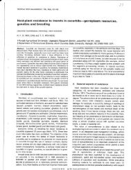
Journal of Heredity 2007:98(4):345–350
doi:10.1093/jhered/esm033
Advance Access publication June 30, 2007
Computer Note
SASQuant: A SAS Software Program
to Estimate Genetic Effects and
Heritabilities of Quantitative Traits
in Populations Consisting of 6 Related
Generations
GABRIELE GUSMINI,TODD C. WEHNER, AND SANDRA
B. DONAGHY
From Syngenta Seeds, Inc., 10290 Greenway Road,
Naples, FL 34114 (Gusmini); Department of Horticultural
Science, North Carolina State University, Raleigh, NC
27695-7609 (Wehner); and Department of Statistics,
North Carolina State University, Raleigh, NC 27695-8203
(Donaghy).
Address correspondence to Todd C. Wehner at the address
above, or e-mail: todd_wehner@ncsu.edu.
Plant breeders are interested in the analysis of phenotypic
data to measure genetic effects and heritability of quantitative
traits and predict gain from selection. Measurement of phenotypic
values of 6 related generations (parents, F1, F2, and
backcrosses) allows for the simultaneous analysis of both Mendelian
and quantitative traits. In 1997, Liu et al. released a SAS
software based program (SASGENE) for the analysis of inheritance
and linkage of qualitative traits. We have developed
a new program (SASQuant) that estimates gene effects (Hayman’s
model), genetic variances, heritability, predicted gain
from selection (WrightÕs and Warner’s models), and number
of effective factors (WrightÕs, Mather’s, and LandeÕs models).
SASQuant makes use of traditional genetic models and allows
for their easy application to complex data sets. SASQuant is
freely available and is intended for scientists studying quantitative
traits in plant populations.
Analysis of phenotypic data for estimating genetic effects,
heritability, and gain from selection for quantitative traits
is an important statistical tool for plant breeders. Quantitative
methods partition the total variance into genetic and environmental
variances and the genetic variance into additive and
dominance components and interallelic interaction effects,
whenever the population structure and composition allows
(Nyquist 1991; Holland et al. 2003). Variance of the F2 provides
an estimate of phenotypic variance, whereas the mean
variance of the nonsegregating generations (P1, P2, and F1)
provides an estimate of environmental variance (Wright
ª The American Genetic Association. 2007. All rights reserved.
For permissions, please email: journals.permissions@oxfordjournals.org.
1968). Additive variance is derived by subtracting the variances
of the backcrosses (B 1,B 2) from twice the phenotypic
(F 2) variance, as an extension of the single-locus model
and assuming absence of linkage and of genotype by environment
interaction (Warner 1952). The broad- and narrowsense
heritabilities and the predicted gain from selection
can then be calculated from the available estimates of genetic,
additive, and phenotypic variances. In addition, main and epistatic
gene effects contributing to the phenotypic expression
of a quantitative trait can be partitioned according to the
model proposed by Hayman (1958) and reviewed by Gamble
(1962).
In 1997, Liu et al. published SASGENE, a program using
SAS software (SAS Institute, Cary, NC), for the analysis of
inheritance and linkage of Mendelian genes. SASGENE
required phenotypic ratings (discreet data) from families
(or crosses) of 6 related generations (parents, F1, F2, and
backcrosses) segregating for the traits of interest (Liu et al.
1997). However, SASGENE did not provide information
on the genetics of quantitative traits segregating in those
same families.
We have developed a new program, called SASQuant, for
the genetic analysis of quantitative data. SASQuant uses the
Output Delivery System (SAS Institute Inc. 2005) of SAS
software (version 8 and higher). SASQuant is dimensioned
for the analysis of an unlimited number of traits and unlimited
number of individuals per generation and family. SAS-
Quant, as required by the genetic models used, combines
summary statistics (means and variances) in order to estimate
genetic factors and their effects. The actual data set used to
generate the estimates presented in the output of SASQuant
is composed only by this summary statistics. Therefore, additional
descriptive statistics, such as standard errors of the
estimates or F-tests for significance of family mean differences,
cannot be computed. This limitation is part of the genetics
models adopted and cannot be overcome. Furthermore,
SASQuant is intended solely as tool for breeders who are interested
in deploying traditional genetic models such as those
presented herein, not as an improvement over such models.
SASQuant is freely available and includes sample data set
and instructions illustrating the use of the 2 macros and
proper data-recording format. It also shows how to set up
data properly for the analysis. The program files (dist.sas
and estim.sas) and the sample data set (data.dat) can
be obtained from the World Wide Web by visiting http://
cucurbitbreeding.ncsu.edu/ and looking under the ‘‘Software’’
category.
Computational Methods
For each cross, SASQuant requires phenotypic data from
multiple individuals of the 2 inbred parents (P1,P2), F1 345

Journal of Heredity 2007:98(4)
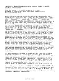
Figure 1. Distribution of F 2 data by Set Family. Output from DIST macro of SASQuant includes data distribution charts for
the F 2 phenotypic values of each trait, which are useful, when visually inspected, to determine whether the data are normally
distributed.
and F2 hybrids, and the 2 backcrosses of the F1 to the parents
(B1,B2). SASQuant analyzes data from multiple phenotyping
experiments (sets), in order to reduce the chances of com-
Table 1. Homogeneity of variance test—Bartlett. Output from
DIST macro of SASQuant includes chi squares and P values to test
for homogeneity of variance of the F2 phenotypic values of each
trait, in order to verify the assumption of equal variance needed to
pool data for a specific source. Bartlett’s test is the default
homogeneity of variance test for the SASQuant program, but
other algorithms can be specified by the user
Dependent Set Family Source df Chi square Probability
Height Set 1 34.4194 ,0.0001
Height Fam 8 53.8471 ,0.0001
Height 17 Set 1 4.5620 0.0327
Height 18 Set 1 6.6999 0.0096
Height 19 Set 1 9.5673 0.0020
Height 20 Set 1 3.7412 0.0531
Height 21 Set 1 0.9134 0.3392
Height 22 Set 1 3.7600 0.0525
Height 23 Set 1 5.3446 0.0208
Height 24 Set 1 3.6507 0.0560
Height 25 Set 1 0.4492 0.5027
Height 01 Fam 8 36.2800 ,0.0001
Height 02 Fam 8 25.4451 0.0013
346
plete loss of valuable and unique populations due to environmental
adversities or disease epidemics at one location. In
addition, sets could be considered as different environments,
in order to reduce environmental effects on genotype. SAS-
Quant analyzes an input data file that consists of plot number,
set number, family number, and generation number,
followed by the trait values. Families and sets can be assigned
characters or numbers. The generation codes required by
SASQuant are P1 5 Ô01Õ, P2 5 Ô02Õ, F1 5 Ô03Õ, F2 5 Ô04Õ,
B1 5 Ô05Õ, and B2 5 Ô06Õ.
SASQuant consists of 2 SAS macros. The first macro,
DIST, plots the data from the F2 generation so that the user
can visually verify the normal distribution of the F2 phenotypic
data. In a second step, the DIST macro tests the homogeneity
of variances of the F2 data overall, by family
over set and by set over family (Ostle and Malone 1988; Steel
et al. 1997). From this analysis, the user can interpret the chi
squares for the null hypothesis of homogeneous variances
and decide how to pool the data for the analysis (overall,
by set, by family, or not pooled). By default, the program
performs Bartlett’s test, but LeveneÕs or any other test of homogeneity
of variances available in SAS can be selected. The
second macro, ESTIM, calculates means and variances by
generation and pooling factor (overall, by set, by family,
or not pooled), as indicated by the user. Generation means

and variances are then combined to estimate genetic variances,
heritabilities (narrow and broad sense), number of effective
factors, predicted gain from selection, and gene effects.
SASQuant estimates phenotypic (P), environmental (E),
genotypic (G), and additive (A) effects from generation variances
as follows (Warner 1952; Wright 1968):
ˆr 2
P 5 ˆr2 F2
ˆr 2
G 5 ˆr2 P
ˆr 2 ˆr2 þ ˆr2 þð2 ˆr2
P1 P2 F1
E 5 Þ
4
ˆr 2
E
ˆr 2
A
5 ð2 ˆr2
F2
Þ ðˆr2 þ ˆr2 B1 B2Þ SASQuant estimates the number of effective factors using
the following 5 methods (Wright 1968; Lande 1981; Mather
and Jinks 1982):
Wright’s method:
ðlP1 lP2Þ2 n
1:5
h
2
lF1 lP2 lP1 lP1 1
lF1 lP2 lP1 lP1 io
8 r2 h i
F2
Mather’s method:
r 2 P 1 þr 2 P 2 þð2 r 2 F 1 Þ
4
ðl P1 l P2 Þ 2
2
ð2 r 2 F2 Þ ðr2 B1 þ r2 B2 Þ
ðl P1
l P2 Þ2
Lande’s method I:
8 r2 h i
F2
ðl P1
r 2 P 1 þr 2 P 2 þð2 r 2 F 1 Þ
4
l P2 Þ2
Computer Note
Table 2. Number of observations and generation means by Set Family. Output from ESTIM macro of SASQuant lists the number of
observations (N) and means (M) by generation (parents, F1, F2, and backcrosses, respectively) for each trait
Set Family NPa MPa NPb MPb NF1 MF1 NF2 MF2 NBCa MBCa NBCb MBCb
01 17 7 16.7 6 54.8 10 33.5 57 30.2 22 24.7 26 43.8
01 18 10 17.2 10 40.8 16 28.8 87 26.7 29 21.8 30 30.2
01 19 8 10.0 7 47.0 13 32.5 92 32.8 22 22.0 29 40.6
01 20 9 10.1 3 23.0 14 27.7 30 27.1 24 18.0 28 36.3
01 21 8 10.9 10 38.8 8 27.9 74 26.0 24 16.7 16 35.1
01 22 3 10.3 3 49.3 10 42.3 48 31.4 15 20.3 17 35.5
01 23 5 5.6 5 44.4 12 20.4 81 20.6 22 11.8 29 30.3
01 24 7 5.1 5 48.0 9 15.8 53 20.5 14 11.9 30 30.1
01 25 6 7.0 5 50.0 10 26.2 45 25.0 17 14.1 29 29.0
02 17 9 12.0 4 39.0 13 23.2 91 26.0 19 20.5 26 29.1
02 18 7 15.9 6 28.7 17 22.8 99 20.2 25 17.8 30 25.8
02 19 8 11.8 4 38.8 17 23.5 106 22.4 29 17.3 27 31.6
02 20 8 8.8 3 32.7 15 18.8 41 20.2 27 16.6 21 24.2
02 21 8 9.4 6 11.8 20 15.5 105 17.7 30 11.1 25 16.0
02 22 9 7.7 5 18.4 12 15.6 102 20.0 26 14.9 24 22.1
02 23 6 3.3 2 30.0 14 11.1 56 15.0 22 8.7 25 25.6
02 24 10 3.3 7 18.7 16 15.8 37 13.5 30 9.3 30 18.3
02 25 10 2.6 5 43.4 18 19.8 64 18.0 30 8.6 24 29.6
Lande’s method II:
8 ½ð2 r2 F2Þ ðr2B1 þ r2B2 ÞŠ
Table 3. Generation variances by Set Family. Output from ESTIM macro of SASQuant lists the variance (Var) by generation (parents,
F1, F2, and backcrosses, respectively) for each trait
Set Family VarPa VarPb VarF1 VarF2 VarBCa VarBCb
01 17 6.57 90.97 54.50 118.20 40.51 106.18
01 18 15.29 82.40 153.76 114.34 54.67 79.22
01 19 12.57 145.00 50.77 139.11 32.10 62.26
01 20 3.61 21.00 24.84 86.82 54.30 81.32
01 21 1.84 28.40 27.55 54.53 36.23 179.72
01 22 0.33 81.33 58.68 111.23 35.50 180.51
01 23 0.80 46.80 22.63 56.86 16.66 68.36
01 24 0.48 172.00 21.44 63.60 27.82 49.17
01 25 7.60 44.50 31.96 62.20 13.11 86.29
02 17 12.25 107.33 58.36 71.09 34.15 82.71
02 18 11.14 11.87 54.53 66.47 45.27 51.43
02 19 17.36 112.92 39.89 74.20 47.71 40.10
02 20 3.36 121.33 62.17 44.59 31.10 88.89
02 21 1.41 32.57 40.89 44.39 15.91 86.79
02 22 3.00 30.80 70.45 69.23 39.39 137.59
02 23 0.27 8.00 42.29 31.55 13.08 110.67
02 24 0.68 45.24 25.80 34.76 13.25 38.56
02 25 0.27 40.30 39.48 51.63 12.52 67.81
347

Journal of Heredity 2007:98(4)
Table 4. Genetic variances and heritability by Set Family. Output from ESTIM macro of SASQuant lists genetic variances (phenotypic,
environmental, genotypic, additive, and dominance, respectively) and broad- and narrow-sense heritability for each trait
Set Family VarP VarE VarG VarA VarD HerB HerN
01 17 118.20 51.63 66.57 89.71 23.14 0.56 0.76
01 18 114.34 101.30 13.03 94.78 81.75 0.11 0.83
01 19 139.11 64.78 74.33 183.87 109.5 0.53 1.32
01 20 86.82 18.57 68.25 38.02 30.23 0.79 0.44
01 21 54.53 21.34 33.20 106.9 140.08 0.61 1.96
01 22 111.23 49.76 61.47 6.45 55.02 0.55 0.06
01 23 56.86 23.21 33.65 28.70 4.95 0.59 0.50
01 24 63.60 53.84 9.76 50.21 40.45 0.15 0.79
01 25 62.20 29.00 33.20 25.01 8.19 0.53 0.40
02 17 71.09 59.08 12.01 25.31 13.30 0.17 0.36
02 18 66.47 33.02 33.45 36.23 2.78 0.50 0.55
02 19 74.20 52.51 21.68 60.58 38.90 0.29 0.82
02 20 44.59 62.26 17.67 30.81 13.14 0.40 0.69
02 21 44.39 28.94 15.44 13.93 29.38 0.35 0.31
02 22 69.23 43.67 25.55 38.53 64.08 0.37 0.56
02 23 31.55 23.21 8.34 60.67 69.00 0.26 1.92
02 24 34.76 24.38 10.38 17.70 7.32 0.30 0.51
02 25 51.63 29.88 21.75 22.94 1.18 0.42 0.44
ðl P1
l P2 Þ2
Lande’s method III:
½8 ðr2 B1 þ r2B2 r2F1 ÞŠ
ðr 2 P 1 þr 2 P 2 Þ
2
SASQuant predicts gain from one cycle of selection as h2 ffiffiffiffiffi
n
r2 P
p
multiplied by the selection differential in standard deviation
units (k) for selection intensities of 5%, 10%, or 20%
(Hallauer and Miranda 1988). The user can modify k to predict
gain from one cycle of selection under a different magnitude
of selection intensity.
SASQuant partitions additive, dominance, and epistatic
effects based on the Hayman’s mean separation analysis procedure
(Hayman 1958; Gamble 1962), using the following
formulae, and computes the standard errors for the estimates
as square root of their variances:
m 5 l F2 a 5 l B1 l B2
d 5 l P1
2
l P2
2 þ l F1 ð4 l F2 Þþ½2 ðl B1 þ l B2 ÞŠ
aa 5 ð4 l F1 Þþ½2 ðl B1 þ l B2 ÞŠ
l B2
ad 5 lP1 2 þ lP2 2 þ lB1 dd 5 lP1 þ lP2 þð2 lF1Þþð4 lF2Þ ½4 ðlB1 þ lB2ÞŠ SASQuant tests the hypothesis that the estimates are significantly
different from zero, performing a Fisher’s t-test. The
estimates a, d, aa, ad, and dd are obtained by combining the
means of generations with different sample sizes (number of
Table 5. Effective factors and gain from selection by Set Family. Output from ESTIM macro of SASQuant lists the number of
estimated effective factors (EF) (Wright’s, MatherÕs, three Lande’s, and average estimates) and the predicted gain from selection (GS)
(selection intensity of 5%, 10%, and 20%, respectively) for each trait
Set Family EF1 EF2 EF3 EF4 EF5 EFm GS05 GS10 GS20
01 17 2.7 8.1 2.7 2.0 4.2 4.0 17.0 14.5 11.6
01 18 5.3 2.9 5.3 0.7 1.0 2.7 18.3 15.6 12.4
01 19 2.4 3.7 2.3 0.9 4.9 0.9 32.1 27.4 21.8
01 20 0.8 2.2 0.3 0.5 0.2 0.8 8.4 7.2 5.7
01 21 3.0 3.6 2.9 0.9 0.6 0.4 29.8 25.5 20.3
01 22 3.7 117.9 3.1 29.5 1.6 31.2 1.3 1.1 0.9
01 23 5.7 26.2 5.6 6.6 4.9 9.8 7.8 6.7 5.3
01 24 26.5 18.3 23.5 4.6 7.5 13.1 13.0 11.1 8.8
01 25 7.0 37.0 7.0 9.2 5.6 13.1 6.5 5.6 4.4
02 17 7.7 14.4 7.6 3.6 70.9 7.5 6.2 5.3 4.2
02 18 0.6 2.3 0.6 0.6 0.7 0.9 9.2 7.8 6.2
02 19 4.2 6.0 4.2 1.5 5.3 2.1 14.5 12.4 9.8
02 20 4.1 9.3 4.0 2.3 15.8 7.1 9.5 8.1 6.5
02 21 0.4 0.2 0.0 0.1 0.0 0.0 4.3 3.7 2.9
02 22 0.6 1.5 0.6 0.4 0.2 0.1 9.5 8.1 6.5
02 23 11.6 5.9 10.7 1.5 1.1 3.2 22.3 19.0 15.1
02 24 3.4 6.7 2.9 1.7 9.7 4.9 6.2 5.3 4.2
02 25 9.7 36.3 9.6 9.1 10.1 14.9 6.6 5.6 4.5
348

individuals rated per generation). Thus, the computation of
the degrees of freedom (df) to be used to fit the t-test is not
obvious. The most conservative approach would be to calculate
the df based on the minimum number of observations
(n) common to all the generations that contribute to the estimates
of each gene effect. For example, if a was estimated
using 30 observations for one backcross generation and
35 for the other, then df should be equal to 29. However,
n is typically largely unbalanced between nonsegregating
(parents and F1) and segregating generations (F2 and backcrosses).
Thus, the df of estimates built from generations
of the 2 groups would use only few observations, and the
t-test would have little power. According to a common prac-
tice among breeders (personal communications), SASQuant
estimates the df as an average of the segregating generations
used to estimate the gene effect, as follows:
dfm 5 nF2 1
dfa 5 dfaa 5 df ad 5
dfd 5 dfdd 5
nB1 þ nB2
2
nF2 þ nB1 þ nB2
3
Computer Note
Table 6. Hayman’s main gene effects by Set Family. Output from ESTIM macro of SASQuant lists HaymanÕs estimates of main gene
effects, their standard errors (SEs), and Student’s t significance level (PROB) (mean, additive, and dominance effects, respectively) for each
trait
Set Family m SEm a SEa Pa d SEd Pd
01 17 30.21 1.44 19.09 3.38 0.0000 13.79 17.28 0.4284
01 18 26.68 1.15 8.44 3.00 0.0087 2.85 15.74 0.8568
01 19 32.79 1.23 18.55 2.67 0.0000 2.11 15.14 0.8895
01 20 27.07 1.70 18.24 3.21 0.0000 11.55 16.19 0.4815
01 21 25.99 0.86 18.46 4.58 0.0007 2.67 15.53 0.8637
01 22 31.44 1.52 15.20 4.80 0.0063 1.81 20.88 0.9313
01 23 20.63 0.84 18.54 2.41 0.0000 2.94 11.27 0.7951
01 24 20.45 1.10 18.21 2.69 0.0000 8.76 14.37 0.5449
01 25 25.02 1.18 14.88 2.60 0.0000 16.15 13.75 0.2464
02 17 25.96 0.88 8.60 3.12 0.0117 6.99 15.08 0.6439
02 18 20.23 0.82 8.01 2.65 0.0056 6.69 11.71 0.5694
02 19 22.37 0.84 14.28 2.50 0.0000 6.47 13.27 0.6269
02 20 20.24 1.04 7.65 3.13 0.0227 1.22 15.97 0.9394
02 21 17.74 0.65 4.91 2.59 0.0693 11.73 10.59 0.2705
02 22 20.04 0.82 7.24 3.63 0.0573 3.59 14.50 0.8051
02 23 15.02 0.75 16.88 2.88 0.0000 2.89 11.60 0.8042
02 24 13.46 0.97 9.00 1.80 0.0000 6.11 10.14 0.5511
02 25 17.98 0.90 21.03 2.33 0.0000 1.29 11.23 0.9089
The output of DIST includes the distribution plots of
data from the F 2 families (Figure 1) and a table of tests of
Table 7. Hayman’s epistatic gene effects by Set Family. Output from ESTIM macro of SASQuant lists HaymanÕs estimates of epistatic
gene effects, their corresponding standard errors (SEs), and Student’s t significance level (PROB) (additive additive, additive
dominance, and dominance dominance effects, respectively) for each trait
Set Family aa SEaa Paa ad SEad Pad dd SEdd Pdd
01 17 16.06 12.52 0.2081 0.03 5.81 0.9962 14.41 28.80 0.6200
01 18 2.66 10.58 0.8026 3.36 5.05 0.5113 14.23 26.88 0.5990
01 19 6.07 10.26 0.5571 0.05 5.58 0.9927 2.89 25.37 0.9098
01 20 0.39 13.22 0.9768 11.80 4.85 0.0224 20.50 25.58 0.4300
01 21 0.36 12.59 0.9772 4.50 5.66 0.4370 2.20 27.63 0.9368
01 22 14.28 15.68 0.3712 4.30 7.57 0.5786 47.07 35.66 0.1985
01 23 1.65 8.16 0.8410 0.86 4.14 0.8365 5.02 19.18 0.7948
01 24 2.04 9.76 0.8361 3.22 5.75 0.5817 1.19 24.35 0.9615
01 25 13.85 9.91 0.1726 6.62 4.66 0.1694 37.02 22.80 0.1151
02 17 4.72 9.78 0.6317 4.90 6.30 0.4453 3.08 26.62 0.9083
02 18 6.12 8.59 0.4791 1.60 3.99 0.6912 3.01 20.15 0.8820
02 19 8.19 8.35 0.3310 0.78 5.89 0.8957 8.30 23.20 0.7221
02 20 0.69 10.43 0.9480 4.31 6.63 0.5221 3.33 27.77 0.9054
02 21 16.62 7.78 0.0374 3.68 3.97 0.3622 14.49 18.58 0.4390
02 22 6.14 10.55 0.5632 1.87 5.15 0.7194 10.65 25.70 0.6804
02 23 8.41 8.75 0.3434 3.54 3.98 0.3826 21.28 20.19 0.2995
02 24 1.36 7.47 0.8565 1.29 3.20 0.6891 3.05 16.41 0.8539
02 25 4.51 8.25 0.5874 0.63 3.83 0.8716 4.59 18.87 0.8089
1
1
349

Journal of Heredity 2007:98(4)
homogeneity of variances (Table 1). For example, the tests of
homogeneity of variances in Table 1 indicate whether the
data can be pooled as follows: 1) all data (tests 1 and 2), using
sets and families as sources for the test, 2) data from all sets
for a specific family (tests 3–11), and 3) data from all families
for a specific set (tests 12 and 13). The output of ESTIM
includes 6 tables (Tables 2–7) reporting the following: number
of observations and means by generation (Table 2), variances
by generation (Table 3), estimates of genetic variances
and heritability (Table 4), number of effective factors and
predicted gain from selection (Table 5), and Hayman’s gene
effects (Tables 6 and 7).
Formulas used by SASQuant may produce negative estimates,
which should be considered equal to zero (Robinson
et al. 1955). Both negative and positive estimates should be
reported to permit unbiased estimates of genetic parameters
in future meta-analysis or, as originally stated, ‘‘in order to
contribute to the accumulation of knowledge, which may,
in the future, be properly interpreted’’ (Dudley and Moll
1969). Furthermore, when a negative estimate results from
derivation from another negative value (e.g., narrow-sense
heritability and gain from selection, calculated from negative
additive variance), it should be omitted.
References
Dudley JW, Moll RH. 1969. Interpretation and use of estimates of heritability
and genetic variances in plant breeding. Crop Sci. 9:257–262.
Gamble EE. 1962. Gene effects in corn (Zea mays L.). I. Separation and relative
importance of gene effects for yield. Can J Plant Sci. 42:339–348.
Hallauer AR, Miranda JB. 1988. Quantitative genetics in maize breeding.
2nd ed. Ames (IA): Iowa State University Press.
350
Hayman BI. 1958. The separation of epistatic from additive and dominance
variation in generation means. Heredity. 12:371–390.
Holland JB, Nyquist WE, Cervantes-Martinez CT. 2003. Estimating and
interpreting heritability for plant breeding: an update. Plant Breed Rev.
22:9–113.
Lande R. 1981. The minimum number of genes contributing to quantitative
variation between and within populations. Genetics. 99:541–553.
Liu JS, Wehner TC, Donaghy SB. 1997. SASGENE: a SAS computer
program for genetic analysis of gene segregation and linkage. J Hered. 88:
253–254.
Mather K, Jinks JL. 1982. Biometrical genetics. The study of continuous variation.
3rd ed. London: Chapman and Hall.
Nyquist WE. 1991. Estimation of heritability and prediction of selection response
in plant populations. CRC Crit Rev Plant Sci. 10:235–322.
Ostle B, Malone LC. 1988. Statistics in research. 4th ed. Ames (IA): Iowa
State University Press.
Robinson HF, Comstock RE, Harvey PH. 1955. Genetic variances in open
pollinated varieties of corn. Genetics. 40:45–60.
SAS Institute Inc. 2005. SAS OnlineDocÒ Version 8. [Internet]. SAS Institute
Inc. Available from: http://www.sas.com/
Steel RGD, Torrie JH, Dickey DA. 1997. Principles and procedures
of statistics: a biometrical approach. 3rd ed. Boston (MA): WCB/
McGraw-Hill.
Warner JN. 1952. A method for estimating heritability. Agron J. 44:
427–430.
Wright S. 1968. The genetics of quantitative variability. In: Wright S, editor.
Evolution and genetics of populations. 2nd ed. Volume 1. Chicago (IL):
University of Chicago Press. p. 373–420.
Received January 25, 2006
Accepted April 19, 2007
Corresponding Editor: William Tracy